ALM models based on second order stochastic dominance · 2018-06-25 · ALM models based on second order stochastic dominance 191 models; a benchmark distribution of funding ratio

Comput Manag Sci (2018) 15:187–211https://doi.org/10.1007/s10287-018-0299-8

ORIGINAL PAPER

ALM models based on second order stochasticdominance

Maram Alwohaibi1 · Diana Roman2

Received: 14 November 2016 / Accepted: 7 February 2018 / Published online: 8 March 2018© The Author(s) 2018. This article is an open access publication

Abstract We propose asset and liability management models in which the risk ofunderfunding is modelled based on the concept of stochastic dominance. Investmentdecisions are taken such that the distribution of the funding ratio, that is, the ratioof asset to liabilities, is non-dominated with respect to second order stochastic dom-inance. In addition, the funding ratio distribution is close in an optimal sense to auser-specified target distribution. Interesting results are obtained when the target dis-tribution is degenerate; in this case,we can obtain equivalent riskminimisationmodels,with risk defined as expected shortfall or as worst case loss. As an application, weconsider the financial planning problem of a defined benefit pension fund in SaudiArabia.

1 Introduction and motivation

To solve a pension fund’s asset and liability management (ALM) problem means todetermine decisions on one or more among the following: allocation of the assets,contributions rate, level of payments, which are optimal in some sense. Usually, theobjective is long term increase in wealth while satisfying solvency requirements at alltimes. The solvency of a fund is measured by the funding ratio, that is, the ratio ofassets to liabilities (Gallo 2009).

The outcome of such decisions depends on parameters whose future value is notknownwith certainty at decision time; such parameters include asset returns, future lia-

B Maram [email protected]

1 Department of Mathematics, Brunel University London, Uxbridge UB8 3PH, UK

2 Brunel University College of Engineering Design and Physical Sciences, London, UK

123

http://crossmark.crossref.org/dialog/?doi=10.1007/s10287-018-0299-8&domain=pdf

http://orcid.org/0000-0002-1873-7911

188 M. Alwohaibi, D. Roman

bilities and contributions. In the stochastic programming (SP) approach, the stochasticprocesses of interest are discretized and represented through a finite set of scenarios.

While pure asset allocation problems are usually modelled as single period, in thecase when liabilities are present, a multi-stage setting is adopted.The basic concepts of ALM models using Stochastic Programming were developedby Kallberg et al. (1982) and Kusy and Ziemba (1986), please also see Pirbhai et al.(2003) and references within. The first commercial application of an asset-liabilitymodel was reported in the literature by Carino et al. (1994) and Carino and Ziemba(1998) for the second largest Japanese insurance company. Other examples includeConsigli and Dempster (1998), Mulvey et al. (2000), Dempster et al. (2003), Geyerand Ziemba (2008), Dupacová and Polívka (2009) and de Oliveira et al. (2017).

Different approaches for modelling risk in the context of ALM can be found inthe literature. They mainly stem from the single period asset allocation modellingframework, where the most common approach is to find investment decisions whichresult in a return distribution with a high expected value and low value of risk. Riskcan be defined in a variety of ways depending on which unfavorable aspect of thereturn distribution is to be penalised. Decisions are then found as optimal solutionsin models where expected value is maximised with a constraint on risk; alternatively,risk can be minimised with a constraint on expected value.

This modelling approach has been extended to the case of multi-period setting,liability driven investment by maximising the expected terminal fund wealth whileimposing risk constraints in the intermediate time periods. When modelling risk inan ALM context, the distribution of interest is not necessarily that of wealth or assetreturn, as the relationship to liabilities is crucial. Instead, the distribution of interestis usually related to the funding ratio. Usually, a target funding ratio is set, a numberλ ≥ 1 below which the value of the funding ratio is desired not to fall. Other said, theundesirable situations are those in which the asset value falls below the liability value(multiplied by λ).

Fishburn (1977) used Lower Partial Moments (LPMs) in the context of single stageasset allocation models. The LPM with target τ and order n of a random variable R(e.g. representing future return) is by definition E[max{τ − R, 0}n]. In the particularcase n = 0, the LPM measures the probability of falling below target τ , which hadbeen used in asset allocation models by Roy (1952).

For multi-stage ALM models, Dert (1995) proposed a similar approach in con-trolling the risk of underfunding, using the stochastic programming paradigm ofchance constraint programming (Charnes and Cooper 1959). Chance constraints wereimplemented recently in a multistage SP for the Brazilian pension fund industry inde Oliveira et al. (2017). Omitting the time index, denote by A the distribution ofasset value and by L the distribution of liabilities. The constraint A ≥ λL underall scenarios is relaxed by allowing a small percentage of scenarios β = B% underwhich underfunding may happen. Formally, Prob(A − λL < 0) ≤ β or equivalentlyProb(A/L < λ) ≤ β. This is the same with imposing an upper limit β on the lowerpartial moment with target λ and order 0 of the random variable A/L representing thefunding ratio.

Chance constraints control the probability of constraint violation but do not accountfor the amount by which it is violated. In addition, they require binary variables to be

123

ALM models based on second order stochastic dominance 189

implemented, thus increasing computational complexity.An alternative SP approach isthe Integrated Chance Constraint Programming (ICCP), proposed by Klein Haneveld(1986) and Klein Haneveld and Van Der Vlerk (2006), used in the context of ALM byKleinHaneveld et al. (2010).With the above notations, an ICCPconstraint requires thatE[max{λL − A, 0}] ≤ θ , where θ is the maximum amount of average underfundingthat a decision maker accepts. This is the same with imposing an upper limit θ on thelower partial moment with target 0 and order 1 of the random variable A − λL .

Risk control in ALMmodels via Lower partial moments of order two has been adoptedby Kouwenberg (2001): E([max{λL − A, 0}]2) ≤ θ .

Conditional Value-at-Risk (CVaR) was proposed by Rockafellar and Uryasev(2000) in the context of single stage asset allocation. Let a random variable (represent-ing loss) and a number α = A% representing a percentage of worst case outcomes.CVaR at confidence level (1−α)measures, largely speaking, “the average of losses inthe worst A% of cases”. In the context of multi-stage ALM, it was used by Bogentoftet al. (2001); they considered the loss variable λL − A and imposed an upper limit onits CVaR.

The approaches above are thus related to themean-risk paradigm, often employed inasset allocation due to its intuitive setting and, in most cases, computational simplicity.On the other hand, in imposing risk constraints, one single aspect of the distribution ofinterest is controlled. For example, a limit on the expected shortfall does not guaranteemanageable worst case realisations and hence does not exclude the possibility of catas-trophic losses; a distribution might have a very small percentage of very low outcomesand high outcomes in the rest; in this case, an integrated chance constraints may besatisfied but the worst case realisation could be unacceptably low. Similarly, a CVaRupper limit may guarantee manageable outcomes even under worst case scenarios, butit may leave open the possibility of under-achievement in the rest of the distribution.For instance, a distribution may be “flat” in that the worst case realisations are notvery low, but with little improvement in the rest of the distribution.

In this paper, we propose an alternative way of controlling the risk of underfunding,using the concept of Second Order Stochastic Dominance (SSD). This is a criterion ofranking random variables that takes the entire distribution of outcomes into account.It is applied to random variables whose outcomes are desired to be high and for whoman increase is more valued if it is at low levels, rather than at high levels; typical suchrandom variables represent return or wealth. SSD eliminates the need to specify a util-ity function but works under the general and widely accepted assumptions of decisionmakers being rational (utility function is non-decreasing) and risk averse (utility func-tion is concave). By definition, a random variable is preferred to another with respectto SSD if its expected utility is higher, for any non-decreasing and concave utilityfunction. It is obviously desirable to eliminate the random variables that are domi-nated and make a choice among the SSD non-dominated ones, possibly employinganother criterion to help in the final selection.The conceptual advantages of using SSD in asset allocation has been long recog-nised, along with computational difficulties in applying it (Whitmore and Findlay1978). Recently, computationally tractable optimisation models based on SSD havebeen proposed for single stage portfolio optimisation—for example, Dentcheva andRuszczynski (2006), Roman et al. (2006), Fábián et al. (2011a, b), Post and Kopa

123


(2013), Kopa and Post (2015) and very recently for multistage SP problems-see forexample Escudero et al. (2016) and Kopa et al. (2018).

In the optimisationmodels proposed in this paper, decision variables represent port-folio rebalancing decisions. SSD is used as a choice criterion for random variablesrepresenting funding ratios. The approaches developed in Roman et al. (2006) andFábián et al. (2011b) are extended and adapted to the ALM multi-period case, takinginto account the relationship between asset value and liabilities. An optimal solutionhas a corresponding funding ratio distribution that is SSD non-dominated; in addition,it comes close, in well defined sense, to a target distribution of funding ratio, whoseoutcomes are specified by the decision maker. Different target distributions lead to dif-ferent SSDefficient solutions.A constraint on the expected terminalwealth is imposed,by considering a minimum acceptable compounded return. Improved distributions offunding ratios may be thus achieved, compared to the existing risk models for ALM.This represents the first contribution of the paper. The second contribution is of theo-retical nature; interesting results, connecting the proposed models to well establishedrisk models and well established classes of SP models are derived for the particularcase when the target distribution is deterministic, specified by one single outcome.

Previously, SSD has been used in multi-stage ALM models by Yang et al. (2010),by imposing a stochastic dominance constraint: the objective is themaximise expectedterminal wealth, while the distribution of asset value is constrained to dominate, withrespect to SSD, a given benchmark distribution.More recently,Kopa et al. (2018) applyfirst and second order stochastic dominance constraints in a multistage SP model forindividual optimal pension allocation. The objective is to minimize the Average Valueat Risk Deviation measure while satisfying a wealth target; the optimum portfolio isconstrained to dominate a benchmark with respect to stochastic dominance relations.In our approach, the the SSD criterion is applied to funding ratio distributions and inthe objective, rather than as a contraint. This overcomes undesirable situations thatmight occur, depending on the benchmark distribution chosen by the decision maker.For example, if the outcomes of the benchmark distribution are too high and as a resultthis distribution cannot be dominated or attained, a stochastic dominance constraintwould result in infeasibility. In the opposite situation when the benchmark distributionis SSD dominated, the optimal solution is guaranteed to improve on the benchamarkbut not necessarily to be SSD non-dominated.

With the family of models proposed in this paper, there are three possible cases.Firstly, if the benchmark distribution is dominated with respect to SSD, the optimalsolutionl results in a funding ratio distributionwhich is “better than target”: it improveson the benchmark until SSD efficiency is attained. Secondly, if the benchmark is SSDefficient, the optimal solution of the model has a funding ratio distribution that exactlymatches the benchmark. Finally, if the target is not attainable (in the sense that nofeasible solution could match or improve on it), the optimal solution has a fundingratio distribution which is SSD efficient and comes as close as possible, in a welldefined sense, to the target.

The rest of this paper is organised as follow. In the next section we set a basic frame-work for anALMdecision problemand recallmain riskmodelling frameworks: chanceconstraint programming, integrated chance constraint programming, ConditionalValue-at Risk. Section 3 presents the mathematical formulation of the proposed SSD

123


models; a benchmark distribution of funding ratio is assumed to be available. Section4 presents the connection with the ICCP formulation and more generally, the mean-risk framework, for the particular case when the benchmark distribution is degenerate.A numerical experiment is presented in Sect. 5, using a dataset drawn from a largedefined benefit pension fund in Saudi Arabia. Conclusions are presented in Sect. 6.

2 ALM problem setting

We consider a pension fund problem in which the planning horizon is split into Tsub-periods. At each time point t ∈ {0, . . . , T − 1} a decision is made on rebalancingthe portfolio allocations. At each of these time points, liabilities are to be paid out andcontributions are to be paid in.

The returns of the available assets, as well as values of liabilities and contributionsare observed at times t ∈ {1, . . . , T }. The uncertainty about asset returns, liabilitiesand contributions is modelled by a set of S sample paths, or scenarios. Each scenariohas an associated probability of occurrence πs,∀s ∈ {1, . . . , S}, where πs > 0 and∑S

s=1πs = 1. Similarly to Bogentoft et al. (2001), we consider a scenario tree in theform of a fan; the root node represents the present (t = 0) when first stage decisionsabout portfolio rebalancing need to be taken. Each path from t = 0 to t = T representsone scenario, that is, one possible sequence of outcomes of the stochastic elementsthroughout the time horizon under consideration. The fund’s total value of assets isevaluated at time T ; in the intermediate time periods, risk constraints are imposed,usually related to the funding ratio not being lower than a pre-specified target levelλ ≥ 1. Values of λ > 1 often are used to add some extra safety margin.

In what follows, we present the basic modelling framework. We use the followingnotations:

I = number of financial assets available for investmentT = number of time periodsS = number of scenarios

The parameters of the model are denoted by:

Lt,s = Liability value for time period t under scenario s; t = 1 . . . T , s = 1 . . . SCt,s = The contributions paid into the fund at time period t under scenario s;

t = 1 . . . T , s = 1 . . . SRi,t,s = The rate of return of asset i at time period t under scenario s; i = 1 . . . I,

t = 1 . . . T , s = 1 . . . Sπs = The probability of scenario s occurring; s = 1 . . . S

OPi = The amount of money held in asset i at the initial time period t = 0;i = 1 . . . I

ψ = The transaction cost expressed as a percentage of the value of each tradeL0 = Aggregated liability payments to be made “now” (t = 0)C0 = The funding contributions received “now” (t = 0)

Let us denote the first stage decision variables by:

Bi,0 = The monetary value of asset i bought at the beginning of the planninghorizon (t = 0); i = 1 . . . I

123


Si,0 = The monetary value of asset i sold at t = 0; i = 1 . . . IHi,0 = The monetary value of asset i held at t = 0; i = 1 . . . I

with Hi,0 = OPi + Bi,0 − Si,0, i = 1 . . . I.

Let us denote the recourse decision variables by:

Hi,t,s = The monetary value of asset i held at time t under scenario s; i = 1 . . . I ,t = 1 . . . T , s = 1 . . . S

Bi,t,s = The monetary value of asset i bought at time t under scenario s; i = 1 . . . I ,t = 1 . . . T − 1, s = 1 . . . S

Si,t,s = The monetary value of asset i sold at time t under scenario s; i = 1 . . . I ,t = 1 . . . T − 1, s = 1 . . . S

Denote by At,s the total asset value at time t under scenario s, before portfoliorebalancing. The following relations hold:

At,s =I∑

i=1

Hi,t−1,s Ri,t,s, t = 2 . . . T − 1, s = 1 . . . S

A1,s =I∑

i=1

Hi,0Ri,1,s, s = 1 . . . S

At each time point t ∈ {1, . . . , T }, the asset value At and the liability value Lt

are random variables with outcomes {At,s}s=1...S and {Lt,s}s=1...S , occurring withprobabilities {πs}s=1...S .

The common approach encountered in the literature is to maximise the expectedvalue of the terminal asset value AT while imposing risk constraints on short ormedium term. The funding ratio at time t, denoted here by Ft and defined as At/Lt

is commonly used to model risk constraints, although there are variations in the waythese aremodelled. Ideally, wewould like At ≥ λLt , or Ft ≥ λwith probability 1; thishowever might be impossible and/or very costly for the long term wealth of the fund.

Dert (1995) used a chance constraint, imposing instead At ≥ λLt with high (pre-specified) probability. Such a constraint ismodelled using S additional binary variablesfor every time period when a chance constraint is imposed. The binary variables countthe number of times the constraint is violated; δt,s = 1 when At,s < λLt,s and 0otherwise.

Chance constraints have no control on the amount of shortfall; there is the possibilityof the amount of underfunding (occurring under low probability) being unacceptablylarge. Klein Haneveld et al. (2010) apply integrated chance constraints (ICCs) formodelling short term risk (t = 1) in an ALM model for Dutch pension funds. Withan ICC, the amount of expected shortfall is controlled, rather than the probability ofshortfall: E[max{λLt − At , 0}] ≤ θ , where θ is the maximum amount of averageunderfunding that a decision maker accepts. This could be equivalently formulated asE[max{λ − Ft , 0}] does not exceed a pre-specified level, hence imposing an upperbound on the lower partial moment of order 1 and target λ of the funding ratio.Modelling such a constraint does not require additional binary variables but onlycontinuous ones; we formulate this in Sect. 4.2.

123


Bogentoft et al. (2001) considered a loss random variable defined by λLt − At

and imposed a CVaR constraint for short term risk (t = 1). If CVaR is considered atconfidence level A% = α ∈ (0, 1) (e.g.α = 0.95) then this constraint can be expressedas follows: the average of the highest (1− A)% outcomes of the loss is no higher thana level pre-specified by the decision-maker. Just as with ICC constraints, a CVaRconstraint is modelled by introducing additional (continuous) variables and linearconstraints; the reader is referred to Rockafellar and Uryasev (2000) and Bogentoftet al. (2001).

We can summarise the difference between an ICC constraint and a CVaR constraintas follows. With ICC constraints, all the outcomes of the funding ratio are considered,in which the target funding ratio is not met. With a CVaR constraint, the percentageof worst case outcomes is fixed in advance; these worst case outcomes may or maynot include all the cases in which the target funding ratio is not met. It can be arguedthat ICC provides a better modelling approach since all scenarios when underfundingoccurs are considered. On the other hand, there is less control in worst case scenarios;although the average underfunding may seem acceptable, the possibility exists for aheavy left tailed loss distribution. This leaves the open question on what risk measureis most appropriate.

An ALM model with a generic risk constraint can be formulated as follows:

maxS∑

s=1

πs AT,s (1)

subject to:

Hi,0 = OPi + Bi,0 − Si,0, i = 1 . . . I (2)

Hi,1,s = Hi,0Ri,1,s + Bi,1,s − Si,1,s, i = 1 . . . I, s = 1 . . . S (3)

Hi,t,s = Hi,t−1,s Ri,t,s + Bi,t,s − Si,t,s, i = 1 . . . I, t = 2 . . . T − 1,

s = 1 . . . S (4)

Hi,T,s = Hi,T−1,s Ri,T,s, i = 1 . . . I, s = 1 . . . S (5)I∑

i=1

Bi,0(1 + ψ) + L0 =I∑

i=1

Si,0(1 − ψ) + C0 (6)

I∑

i=1

Bi,t,s(1 + ψ) + Lt,s = Ct,s +I∑

i=1

Si,t,s(1 − ψ), t = 1 . . . T − 1,

s = 1 . . . S (7)

A1,s =I∑

i=1

Hi,0Ri,1,s, s = 1 . . . S (8)

At,s =I∑

i=1

Hi,t−1,s Ri,t,s, t = 2 . . . T, s = 1 . . . S (9)

123


Bi,0, Si,0, Hi,0, Bi,t,s, Si,t,s, Hi,t,s, Hi,T,s ≥ 0, i = 1 . . . I, t = 1 . . . T − 1,

s = 1 . . . S (10)

ρ(At − λLt ) ≤ θ (11)

Equations (6) and (7) are cash balance constraints. Equation (11) expresses a riskconstraint with a generic risk measure ρ of the random variable At − λLt ; the riskvalue must not exceed a user pre-specified level θ . A common approach is to imposea risk constraint for t = 1 (as per Klein Haneveld et al. 2010; Bogentoft et al. 2001);this can be generalised to include other time periods.

Wepropose an alternative riskmodelling framework based on the concept of SecondOrder Stochastic Dominance (SSD).

3 Second order stochastic dominance in ALM models

SSD is a preference relation among random variables—representing, for example,portfolio returns, or asset values, or funding ratios—defined by the following equiva-lent conditions:

(a) E(U (R)) ≥ E(U (R′)) holds for any utility function U that has the properties ofnon-satiation (it is non-decreasing, first derivative is positive) and risk aversion(it is concave, second derivative is negative) and for which these expected valuesexist and are finite.

(b) E([τ − R]+) ≤ E([τ − R′]+) holds for each target τ ∈ R. Other said, theexpected shortfall with respect to any target is always lower for the first randomvariable.

(c) Tailα(R) ≥ Tailα(R′) holds for each 0 < α ≤ 1, where Tailα(R) denotes theunconditional expectation of the lowest α ∗ 100% of the outcomes of R.

(d) Scaled Tailα(R) ≥ Scaled Tailα(R′) holds for each 0 < α ≤ 1, whereScaledTailα(R) denotes the conditional expectation of the lowest α ∗ 100% ofthe outcomes of R; Scaled Tailα(R) = 1

αTailα(R).

If the relations above hold, the random variable R is said to dominate the randomvariable R′ with respect to SSD.The equivalence of the above relations was proved in Whitmore and Findlay (1978)and Ogryczak and Ruszczynski (2002); please see also Fábián et al. (2011a).

Remark 1 The definitions of Tailα(R) and ScaledTailα(R) are informal. For formaldefinitions, quantile functions can be used. Denote by FR the cumulative distributionfunction of a random variable R. If there exists t such that FR(t) = α then Tailα(R) =αE(R|R ≤ t) and Scaled Tailα(R) = E(R|R ≤ t)—which justifies the informaldefinitions.

For the general case, let us define the generalised inverse of FR as F−1R (α) :=

inf{t |FR(t) ≥ α} and the second quantile function as F−2R (α) := ∫ α

0 F−1R (β)dβ

and F−2R (0) := 0. Then, Tailα(R) := F−2

R (α).

123


The relationship with Conditional Value at Risk (CVaR) has been discussed in theliterature in Kopa and Chovanec (2008) and later on in Fábián et al. (2011a). Assumingloss is described by the random variable −R, we have:Tailα(R) := −αCVaR1−α(−R) and ScaledTailα(R) := −CVaR1−α(−R).

Remark 2 The relation in point (b) shows the connection between LPM of order 1 andSSD; R dominates R′ with respect to second order stochastic dominance if the LPMof order 1 and target τ of R is smaller than LPM of order 1 of R′ for all targets τ ∈ R.This is a particular case of a more general relationship between stochastic dominanceand LPMs shown in Post and Kopa (2013).

The importance of SSD in financial asset allocation can be clearly seen: it expressesthe preference of rational and risk-averse decision makers.

We propose an ALM model in which the first stage investment decisions are suchthat the resulting funding ratio distribution is non-dominated with respect to SSD, orin other words, SSD efficient. Similarly to Klein Haneveld et al. (2010), we considerthe funding ratio at time t = 1, thus modelling short term risk; the approach can beextended for more time periods.Following Roman et al. (2006), we assume that the probabilities of scenarios areequal, that is πs = 1/S, s = 1 . . . S. This is the usual situation when scenarios aregenerated via simulation or sampled from historical data. In this case, as shown inRoman et al. (2006), Kopa and Chovanec (2008) also used in Fábián et al. (2011a, b),the comparison with respect to SSD can be greatly simplified: for example, in relations(c) and (d) from the definition of SSD, it is enough to consider α only in the finiteset {1/S, 2/S, . . . , S/S} rather than in the interval (0,1). Other said, it is enough tocompare tails only for confidence levels k

S with k = 1 . . . S.

Let us consider two sets of first stage decisions (Hi,0, i = 1 . . . I ) and (H ′i,0, i =

1 . . . I ) with corresponding funding ratios F and F ′ respectively, having as possibleoutcomes

Fs =I∑

i=1

Hi,0Ri,1,s/L1,s, s = 1 . . . S

and

F ′s =

I∑

i=1

H ′i,0Ri,1,s/L1,s, s = 1 . . . S

respectively; each of these outcomes occurs with probability 1/S.

Let us order F1, . . . FS and F ′1, . . . F

′S and lets us denote by α1 ≤ . . . ≤ αS the

outcomes of F in ascending order and β1 ≤ . . . ≤ βS the outcomes of F ′ in ascendingorder. It is clear that:

Tailk/S(F) = (∑k

i=1αi )/S and ScaledTailk/S(F) = (∑k

i=1αi )/k.With the notations here, the relationships developed in Roman et al. (2006) can be

written as:

123


F dominates F ′ with respect to SSD if and only if

Tailk/S(F) ≥ Tailk/S(F′), k = 1 . . . S

or equivalently,

ScaledTailk/S(F) ≥ ScaledTailk/S(F′), k = 1 . . . S

with at least one strict inequality; please also see Kopa and Chovanec (2008).Thus, the SSD efficient solutions are the Pareto non-dominated optimal solutions in

a multi-objective optimisation problem in which the objective functions to maximiseare the tails (or scaled tails) of the funding ratio distribution F , at confidence levelskS , with k = 1 . . . S :

Max(Tail1/S(F),Tail2/S(F), . . . ,TailS/S(F)) (12)

or we can use the “scaled” version:

Max(Scaled Tail1/S(F),Scaled Tail2/S(F), . . . ,Scaled TailS/S(F)) (13)

subject to: (2)–(10).

Remark 3 Due to the relationship between CVaR and scaled tails expresed in Remark1, it can be clearly seen that (13) is equivalent to a multi-objective minimisation modelin which the objective functions are CVaRs at confidence levels (1− 1

S , 1− 2S , . . . , 0).

There are various methods of obtaining a Pareto optimal solution of a multi-objective optimisation problem.Agood control on obtaining a specific solution is givenby the Reference Point Method (Wierzbicki 1982), where target points (also calledreference points) are set for each objective function.Consider the general case of S real-valued objective functions F1, . . . FS defined on a set X ∈ R

n representing a feasibleset of decision vectors and consider themulti-objectivemodel:Max(F1(x), . . . FS(x))s.t. x ∈ X. For each of the functions Fk a target point f ∗

k is set by the decision maker;partial achievements (Fk(x)− f ∗

k ), k = 1 . . . S can bemeasured for any feasible point.In Wierzbicki (1982), it is shown that maximisation of the worst partial achievement,that is, maximisation of Min{F1(x)− f ∗

1 , . . . , FS(x)− f ∗S } results in a Pareto optimal

solution of the multi-objective model, apart possibly from the case of multiple optimalsolutions. To guarantee Pareto efficiency in the general case, a regularization term isadded to the worst partial achievement: ε

∑Sk=1(Fk(x) − f ∗

k ), where ε > 0. It wasshown in Wierzbicki (1982) a Pareto optimal solution of the multi-objective model isobtained for any ε > 0; however, a small enough ε should be chosen (possibly on atrail and error basis) if optimisation of the worst partial achievement is desired.

Similarly to Roman et al. (2006), we use the Reference Point Method in order toobtain Pareto optimal solutions of (13), that is, SSD efficient solutions in the ALMmodel. In our case, the objective functions represent tails or scaled tails (at differentconfidence levels) of the funding ratio distribution. Thus, the target points for eachobjective function define a target, or “reference” distribution of funding ratio.

123


Let us consider a target distribution of the funding ratio, with (equally probable)outcomes λk, k = 1 . . . S; without loss of generality, let us consider λ1 ≤ . . . ≤ λS .

Let us denote by aspk the scaled kth cumulative outcome,

aspk = 1

k

k∑

i=1

λi , k = 1 . . . S

and by asp′k be the unscaled kth cumulative outcome,

asp′k = 1

S

k∑

i=1

λi , k = 1 . . . S

The target point for the kth objective function in (13) is aspk , while asp′k represents

the target point for the kth objective function in (14). FollowingWierzbicki (1982), themulti-objectivemodel (13) is transformed into a single objectivemodel bymaximisingthe following achievement function:

mink=1...S

(Scaled Tailk/S(F) − aspk) + ε

S∑

k=1

(Scaled Tailk/S(F) − aspk)

If the unscaled model is used, the objective function to maximise is:

mink=1...S

(Tailk/S(F) − asp′k) + ε

S∑

k=1

(Tailk/S(F) − asp′k)

In order to express the tails and scaled tails of the funding ratio distribution asfunctions of the decision variables, we adopt the CVaR formulation of Rockafellarand Uryasev in Rockafellar and Uryasev (2000). It expresses a cumulative outcomeof a random variable as the optimal value of an LP model:

Proposition 1 For every k ∈ {1, . . . , S}, the mean of the worst k outcomes of arandom variable y with equally likely outcomes y1, . . . , yS is the optimal value of theobjective function in the following LP problem:

Max

[

Tk − 1

k

S∑

i=1

dk,i

]

Subject to:

Tk − ys ≤ dk,s, s = 1 . . . S

dk,s ≥ 0, k, s = 1 . . . S

Tk is a free variable representing the kth worst outcome of the random variable y.

123


For each s ∈ {1, . . . , S}, dk,s takes value 0 if ys is greater than or equal to the kthworst outcome Tk ; otherwise, dk,s = Tk − ys .For proof, the reader is referred to Rockafellar and Uryasev (2000).

Hence, (13) becomes:

Max

(

T1 −S∑

i=1

d1,i , T2 − 1

2

S∑

i=1

d2,i , . . . , TS − 1

S

S∑

i=1

dS,i

)

Subject to:

Tk − Fs ≤ dk,s, k, s = 1 . . . S

dk,s ≥ 0, k, s = 1 . . . S

Thus, the following SSD scaled model is formulated:

Max δ + ε

(S∑

k=1

Zk −S∑

k=1

aspk

)

Subject to:

Zk = Tk − 1

k

S∑

s=1

dk,s, k = 1 . . . S (14)

Zk − aspk ≥ δ, k = 1 . . . S (15)

Tk − Fs ≤ dk,s, k, s = 1 . . . S (16)

Fs =I∑

i=1

Hi,0Ri,1,s/L1,s (Fs = A1,s/L1,s), s = 1 . . . S (17)

dk,s ≥ 0, k, s = 1 . . . S (18)

1

S

S∑

s=1

AT,s ≥I∑

i=1

OPi (1 + r) (19)

and also subject to (2)–(10).In addition to the decision variables Hi,0, Bi,0, Si,0, Hi,t,s, Bi,t,s, Si,t,s representing

investment decisions, we have additional decision variables whose nature is discussedbelow:

Tk = the kth worst outcome of the funding ratio at time 1, k = 1 …S (free variables);thus, T1, . . . , TS are the outcomes of a random variable equal in distribution to thefunding ratio;

Zk = the mean of the worst k outcomes of the funding ratio = Scaled Tailk/S(F);Zk = (T1 + . . . + Tk)/k, k = 1 . . . S (free variables);

123


δ = mink=1...S(Zk − aspk) = the worst partial achievement (free variable);dk,s are non-negative variables; dk,s = 0 if the funding ratio under scenario s is greater

than or equal to the kth worst funding ratio Tk ; otherwise, dk,s is the differencebetween Tk and the funding ratio Fs ; k, s = 1 . . . S.

In addition to the parameters already discussed representing returns of the assets,liabilities, contributions and initial portfolio, there are parameters which are chosenby the decision maker:

aspk = the target or aspiration level for Zk = Scaled Tailk/S(F), k = 1 . . . S;r > 0 = desired rate of return over the investment horizon;ε > 0 = theweighting coefficient of the regularisation term in the objective function.

For any choice of aspiration levels and of ε > 0, the optimal solution of theabove model represents a first stage decision allocation Hi0, i = 1 . . . A such that thecorresponding funding ratio F , represented by equally probable outcomes Fs, s =1 . . . S, is SSD efficient.

To prove this, let us suppose that this is not true and the funding ratio Fis SSD dominated; this means that there is another feasible decision H∗

i0, i =1 . . . A with a corresponding funding ratio distribution F∗ (denote its outcomes byF∗s , s = 1 . . . S) that dominates F with respect to SSD. That is, Scaled Tailk/S(F∗) ≥

Scaled Tailk/S(F) , k = 1 . . . S with at least one inequality strict, or with nota-tions above Z∗

k ≥ Zk, k = 1 . . . S with at least one inequality strict, whereZ∗k = Scaled Tailk/S(F∗), k = 1 . . . S. Denote by δ∗ = mink=1...S(Z∗

k − aspk). It

follows that δ∗ + ε(∑S

k=1Z∗k − ∑S

k=1aspk) > δ + ε(∑S

k=1Zk − ∑Sk=1aspk).

For each k ∈ {1, . . . , S}, we solve the model:

Max

[

Tk − 1

k

S∑

i=1

dk,i

]

Subject to:

Tk − F∗s ≤ dk,s, s = 1 . . . S

dk,s ≥ 0, k, s = 1 . . . S

and denote by T ∗k , d∗

k,s, s = 1 . . . S the optimal solution. We obtain thus a feasiblesolution for the (SSD scaled)model that results in a strictly better value of the objectivefunction, which is a contradiction.

Remark 4 The sign of the optimal value of δ or of the optimal value of the objectivefunction in (SSD scaled) is an indication of whether the aspiration levels have beenachieved. A strictly positive δ indicates that the aspiration levels have been strictlyimproved upon. If the aspiration distribution is exactly matched, that is, if the opti-mal solution results in a funding ratio distribution whose scaled tails are exactly thereference points, the optimum value of the objective function is 0. Finally, a strictlynegative optimum indicates that there is at least one scaled tail that did not achieve itstarget.

123


By considering unscaled tails in the multi-objective optimisation, we obtain theSSD unscaled model:

Max δ′ + ε

(S∑

k=1

Z ′k −

S∑

k=1

asp′k

)

Subject to:

Z ′k = kTk −

S∑

s=1

dk,s, k = 1 . . . S

Z ′k − asp′

k ≥ δ′, k = 1 . . . S

also subject to (2)–(10) and to (16)–(19).

Remark 5 Both (SSD scaled) and (SSD unscaled) models have (possibly different)optimal solutions such that their distribution of funding ratio is SSD efficient. Themodelling difference resides in how the “closeness” to the target distribution is mea-sured, more precisely, how the shortfalls below target points are penalised. With theunscaled model, the accumulation of outcomes below their targets is penalised, ratherthan the magnitude of the shortfalls, which is more severely penalised in the scaledmodel. This becomes more obvious when the target distribution is degenerate, havingone single possible outcome. It is shown in the next section that, in this case, the scaledmodelmaximises theworst outcome of the funding ratio, i.e. the largest deviation fromthe (single) target point, while the unscaled model minimises the expected shortfallbelow the target, taking thus into account all situations when the target is not achieved.

Remark 6 Both (SSD scaled) and (SSD unscaled) models provide an SSD efficientsolution, irrespective of the aspiration levels chosen by the decision maker; this choicecannot lead to infeasibility either. This follows from the “better than target” prop-erty of the Reference Point Method in multi-objective optimisation. It was shown inWierzbicki (1982) that themaximisation of the achievement function results in a Paretooptimal solution of the multi-objective model irrespective of the reference points cho-sen by the decision maker. If the reference points do not form a Pareto optimal vectorfor the multi-objective model, the maximisation of the achievement function improveson the reference points until Pareto optimality is attained. If the reference points forma Pareto optimal vector, the optimal solution in the maximisation of the achievementfunction results in objective function values equal to the reference points. Finally, if atleast one of the reference points is unattainable/too high, we obtain a Pareto optimalsolution in which the worst difference between objective function values and referencepoints is optimised.

In the current setting, the multiple objective functions represent tails (or scaled tails)of the funding ratio distribution and Pareto optimal solutions represent SSD efficientdistributions. The three cases above relate to whether the target distribution of fundingratio is (1) SSD dominated; (2) SSD efficient or (3) unattainable, in the sense that

123


there is no feasible solution that could attain or improve on all of its tails. In all threecases, the optimal solutions of both scaled and unscaled models are SSD efficient,corresponding to cases (1) better than target; (2) matching the target; (3) coming closeto the target distribution.

4 Connection with risk minimisation

Consider the particular case in which the target level for every outcome of the fundingratio distribution is equal to target funding ratio λ; λ1 = λ2 = . . . = λS = λ. Thismakes the target distribution a degenerate, or deterministic distribution.

4.1 The SSD scaled model

In this case, the aspiration levels for the scaled tails of the funding ratio are also allequal to λ: aspk = λ, ∀k ∈ {1, . . . , S}.

The worst partial achievement δ = mink=1...S(Zk − aspk) corresponds to theworst outcome of the funding ratio distribution. Thus, maximising the worst partialachievement is equivalent to maximising the worst outcome. A minimax mean-riskmodel, in which risk is defined as the maximum possible loss, was proposed by Young(1998), who also showed that such a model can be formulated as an LP.

In our case a similarMaximinmodel can be formulated, which optimises the worstoutcome of funding ratio, subject to a constraint on the expected terminal wealth.

Max δ

Subject to:

Fs ≥ δ, s = 1 . . . S

also subject to (2)–(10), (17) and (19).In case themodel above has a unique optimal solution, SSDefficiency is guaranteed.

However, just as with the general SSDmodel, in case of non-unique optimal solutions,the SSD efficiency is not guaranteed; a regularisation term should be added in theobjective function. The regularisation term in the SSD scaled model is the sum oftails/cumulated outcomes; in order to formulate tails, we need additional S2 variablesdki which adds substantially to the computational complexity. In order to avoid this,we can add in the objective function above a term such as ε

∑Ss=1Fs which brings no

extra computational complexity; we obtain the model Maximin 2:

Max

(

δ + ε

S∑

s=1

Fs

)

Subject to:

Fs ≥ δ, s = 1 . . . S

123


also subject to (2)–(10), (17) and (19).Just as before, ε has to be chosen as a small enough number such that the opti-

misation is basically that of the worst outcome. The optimal solution of this modelwill result in a funding ratio that has the highest “worst” outcome and also the highestexpected value amongst all optimal solutions of (Maximin). Notice that, although thechance of getting an SSD inefficient solution is substantially decreased at no extra com-putational complexity, SSD efficiency is still not guaranteed as there is theoreticallythe possibility that (Maximin 2) has multiple optimal solutions.

Thus, an SSD scaled model in which the reference distribution is degenerate couldbe in most cases written as a maximin model of minimising worst case outcome. Thesingle outcome of the reference distribution is irrelevant.

4.2 The SSD unscaled model

The aspiration levels for the cumulated outcomes of the funding ratio are:asp′k = 1

S kλ,

k = 1 . . . S. As in Sect. 4.1, denote by T1 ≤ . . . ≤ TS the ordered outcomes of thefunding ratio. The worst partial achievement is:

1

Smin

k=1...S(T1 + . . . + Tk − kλ)

As each outcome below λ is penalised, the minimum is achieved for an index j in{1 . . . S} such that Tj ≤ λ ≤ Tj+1.

The worst partial achievement is thus

1

S[(T1 − λ) + . . . + (Tj − λ)] = 1

S

∑

Tk<λ

(Tk − λ)

Thus, maximising the worst partial achievement is equivalent to minimising

1

S

∑

Tk<λ

(λ − Tk)

which is the Lower Partial Moment of order 1 and target λ of the funding ratio, alsocalled the expected shortfall below target λ.

The model that minimises the expected shortfall below target λ can be formulatedas an LP by introducing S additional variables representing the shortage of the fundingratio with respect to target λ under each scenario:

Min1

S

S∑

s=1

Shs

Subject to:

Fs − λ + Shs ≥ 0, s = 1 . . . S

Sht,s ≥ 0, s = 1 . . . S

123


also subject to (2)–(10), (17) and (19).We notice several things here.

First, without the addition of a regularisation term, minimisation of the expectedshortfall is not guaranteed to result in an SSD efficient solution. One case inwhich SSDefficiencymight not occur is the situation when there are multiple optimal solutions; atleast oneof them isSSDefficient but not necessarily all of them.Theother case inwhichSSD efficiency might not occur is when the optimum in the minimisation of expectedshortfall is zero, that is, T1 ≥ λ. In this case the optimal solution may be ANY solutionsuch that the corresponding funding ratio has all outcomes above the target λ. Addinga regularisation term ensures that the optimal solution is improved until SSD efficiencyis achieved—an example of “better than target” situation. However, a regularisationterm as in the SSD unscaledmodel involves the introduction of additional S2 variables.Similarly to the previous subsection, we may add a term in the objective function suchthat, out of all solutions that minimise the expected shortfall below λ, the one withthe highest expected value is chosen:

Min1

S

S∑

s=1

Shs − ε

S∑

s=1

Fs

with ε a small enough number.Secondly, the model that minimises expected shortfall below λ is closely connected

to an ICCP model (Klein Haneveld et al. 2010), in which the integrated chance con-straint penalises shortfalls of the funding ratio distribution with respect to target λ.

The connection is in the following sense. With the former, the expected shortfall is inthe objective and a constraint on the terminal expected asset value is imposed. Withthe latter, the expected shortfall is the left hand side of a constraint, while maximisingterminal expected asset value may be part of the objective. With appropriate choicesof the right hand sides involved, the two models have the same optimal solution. Wegive an example of such a situation in the next section.

5 Numerical experiment

5.1 Dataset, computational set up and motivation

We consider a large defined benefit pension fund in Saudi Arabia, the General Orga-nization for Social Insurance (GOSI) (http://www.gosi.gov.sa).

We consider a planning horizon of 10 years; t = 0 refers to year 2016. We consider16 asset classes: the Saudi equities represented by 15 sectors indices beside cash.Investment decisions have to be taken “now” (t = 0) and then rebalanced everyyear, t = 1 . . . 9. We generate a set of S = 300 sample paths/scenarios for the assetreturns, contributions and liability values at times t = 1 . . . 10. The scenarios forthe asset returns are obtained by bootstrapping from historical data drawn from theSaudi Arabian stock market index (TASI) (https://www.tadawul.com.sa). For the risk-free rate of return (interest rate) we consider the current Saudi Arabian interest rateof 2% following (http://www.tradingeconomics.com/saudi-arabia/interest-rate), and

123

http://www.gosi.gov.sa

https://www.tadawul.com.sa

http://www.tradingeconomics.com/saudi-arabia/interest-rate


assumed that it will stay at this level for the remaining of the investment period. Thescenarios for the liability and contribution values have the same underlying sourceof uncertainty; they are generated based on populations models and a salary model,assuming that a fixed percentages of salaries are to be paid in, as contributions, or out,as liabilities. The dynamics of the pension’s fund population is modelled by a BIDE(Birth, Immigration, Death, Emigration) model (Sandhya 2011). We used historicaldata on GOSI population as an input to this model (http://www.gosi.gov.sa); thatincludes the number of participants, employment and retirement rates for the last 10years, salary average and average salary growth.

We implement the models (SSD-scaled) and (SSD-unscaled) developed in Sect. 3with deterministic and non-deterministic target distributions of funding ratio. As anon-deterministic target distribution, we use a synthetic one with 300 equally likelyscenarios, in each the lowest outcome is 0.9 and there is an increase by 0.0016 undereach scenario. As a deterministic target distribution, we use one defined by the singleoutcome λ = 1.1.

We refer to the SSD scaled model with deterministic target distribution as (Max-imin); as exposed in Sect. 4.1, it is equivalent to a maximisation of the worst fundingratio.

We refer to the SSD unscaled model with deterministic target distribution as ICCP,because it has the same optimal solution as an ICCP of model in which the expectedterminal asset value is maximised and constraint is imposed on the expected shortfallwith respect to λ.We have showed in the previous section that, in case of deterministictarget distribution with a single outcome, the SSD unscaled model reduces to a modelin which the expected shortfall (below the single target) is minimised. If we constrainthe expected shortafall to be below a specified limit (an ICCP type of model) we obtainthe same optimal solutions, provided that the right hand sides are chosen appropriately.In our numerical experiments, we implement an ICCP model in which we maximisethe expected terminal asset value and we constrain the expected shortfall to be nomore than 5% of the lowest scenario value for liability at time 1. We recorded thisoptimal value of the objective function; let us denote it by AT . We implemented theSSD unscaled model with deterministic target 1.1 with a constraint on the expectedterminal asset value: to be no less than AT . The two models have the same optimalsolution.

We have thus four SSD based models that we refer to as (SSD-scaled), (SSD-unscaled), (Maximin) and (ICCP). In all four models, the right hand side of theconstraint on the expected terminal asset value is the same (equal to AT which corre-sponds to a cumulated terminal wealth of 581.5548 billions of Saudi Riyals (SAR)).The value of ε is fixed to 0.0001. We implement the models in AMPL and solve themusing CPLEX 12.5.1.0.

The objective of this computational work is to investigate differences and similari-ties in the quality of solutions obtained with the four models. More precisely, we lookat the performance measures for the resulting return distributions and at the shape ofthe funding ratio distributions obtained in each of the four cases, particularly the lefttails. We investigate whether by appropriately selecting a (non-deterministic) targetdistribution, improved funding ratio distributions can be obtained. Both in-sample andout-of-sample testing are performed.

123



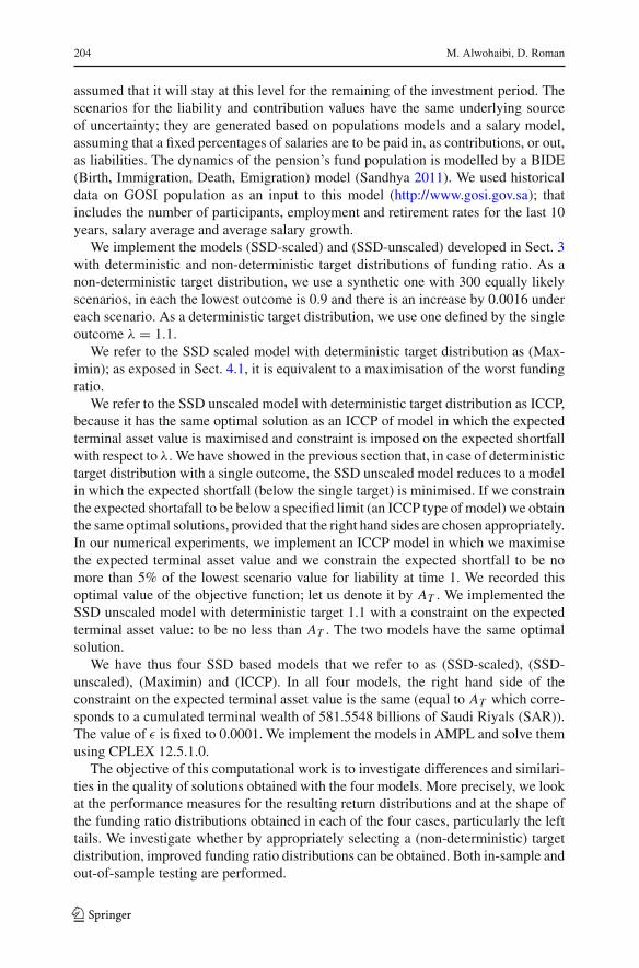
Table 1 Performance measures related to the returns for SSD-unscaled, SSD-scaled, ICCP, and maximinmodels

Comparison criteria SSD-unscaled SSD-scaled ICCP Maximin

Expected rate of return 16.33% 15.72% 14.41% 13.89%

Sharpe ratio 0.7757 0.7158 0.7656 0.7108

Sortino ratio (computed with respectto 0.02% target rate of return)

2.9161 3.8335 2.3188 3.8356

VaR (5%) 0.103 0.085 0.1273 0.07

CVaR (5%) 0.139 0.0922 0.1637 0.0754

All the measures are calculated for the first time period

5.2 Computational results

Table 1 lists statistics and risk-adjusted performance measures of the rate of return ofthe portfolio such as: Sharpe ratio, Sortino ratio, Value at Risk (VaR) and ConditionalValue at Risk (CVaR). For Sharpe and Sortino ratios, the target rate of return is set at2%, that is, excess rate of return and downside risk are calculated with respect to 2%.VaR and CVaR are computed at parameter 5%, that is, considering the worst 5% ofthe outcomes.The results reinforce the similarity between (SSD-unscaled) and (ICCP), as wellas between (SSD-scaled) and Maximin. The rate of returns of the (SSD-unscaled)and (ICCP) solutions have higher expected values and Sharpe ratios but have poorerstatistics regarding left tails/unfavorable outcomes: VaR and CVaR are (much) higher,indicating larger losses under unfavorable scenarios, also the Sortino ratio is consid-erably lower, indicating poorer downside risk return adjusted performance. We noticethat the (SSD-unscaled) solution performs better than the ICCP solution in all reportedmeasures: expected value, risk-adjusted performance measures, left tail statistics.The(SSD-scaled) and (Maximin) solutions are similar in that the statistics on lefttails (as measured by 5% VaR and 5% CVaR) and downside risk are considerablybetter at the expense of average performance. The (Maximin) solution has clearly thereturn distribution with the best left tail, but also with the lowest expected value. The(SSD-scaled) solution provides a compromise between acceptable left tails and higherexpected value.

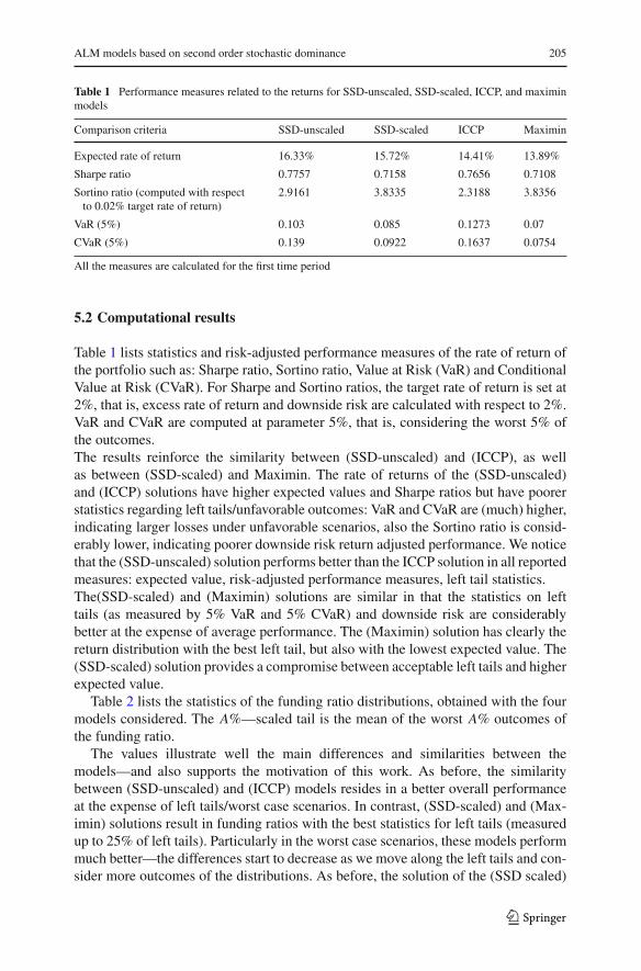
Table 2 lists the statistics of the funding ratio distributions, obtained with the fourmodels considered. The A%—scaled tail is the mean of the worst A% outcomes ofthe funding ratio.

The values illustrate well the main differences and similarities between themodels—and also supports the motivation of this work. As before, the similaritybetween (SSD-unscaled) and (ICCP) models resides in a better overall performanceat the expense of left tails/worst case scenarios. In contrast, (SSD-scaled) and (Max-imin) solutions result in funding ratios with the best statistics for left tails (measuredup to 25% of left tails). Particularly in the worst case scenarios, these models performmuch better—the differences start to decrease as we move along the left tails and con-sider more outcomes of the distributions. As before, the solution of the (SSD scaled)

123


Table 2 Performance measures related to the funding ratio for SSD-unscaled, SSD-scaled, ICCP, andmaximin models


Expected funding ratio 1.160 1.153 1.141 1.135

Minimum funding ratio 0.8168 0.876 0.7926 0.8932

Expected shortfall of FRwith respect to 1.1

0.0455 0.0526 0.0430 0.0517

1%-Scaled tail 0.8200 0.8794 0.7957 0.8967

5%-Scaled tail 0.8526 0.8969 0.8283 0.9124

10%-Scaled tail 0.8725 0.9165 0.8556 0.9290

15%-Scaled tail 0.8946 0.9284 0.8915 0.9392

20%-Scaled tail 0.9207 0.9383 0.9227 0.9471

25%-Scaled tail 0.9420 0.9477 0.9464 0.9551

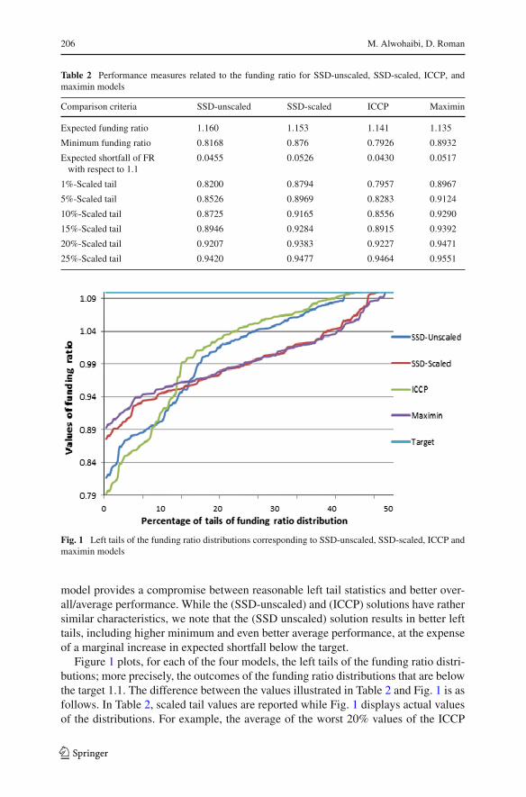
Fig. 1 Left tails of the funding ratio distributions corresponding to SSD-unscaled, SSD-scaled, ICCP andmaximin models

model provides a compromise between reasonable left tail statistics and better over-all/average performance. While the (SSD-unscaled) and (ICCP) solutions have rathersimilar characteristics, we note that the (SSD unscaled) solution results in better lefttails, including higher minimum and even better average performance, at the expenseof a marginal increase in expected shortfall below the target.

Figure 1 plots, for each of the four models, the left tails of the funding ratio distri-butions; more precisely, the outcomes of the funding ratio distributions that are belowthe target 1.1. The difference between the values illustrated in Table 2 and Fig. 1 is asfollows. In Table 2, scaled tail values are reported while Fig. 1 displays actual valuesof the distributions. For example, the average of the worst 20% values of the ICCP

123


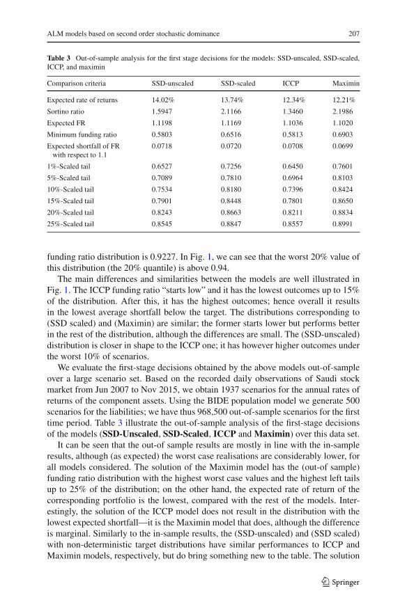
Table 3 Out-of-sample analysis for the first stage decisions for the models: SSD-unscaled, SSD-scaled,ICCP, and maximin


Expected rate of returns 14.02% 13.74% 12.34% 12.21%

Sortino ratio 1.5947 2.1166 1.3460 2.1986

Expected FR 1.1198 1.1169 1.1036 1.1020

Minimum funding ratio 0.5803 0.6516 0.5813 0.6903

Expected shortfall of FRwith respect to 1.1

0.0718 0.0720 0.0708 0.0699

1%-Scaled tail 0.6527 0.7256 0.6450 0.7601

5%-Scaled tail 0.7089 0.7810 0.6964 0.8103

10%-Scaled tail 0.7534 0.8180 0.7396 0.8424

15%-Scaled tail 0.7901 0.8448 0.7801 0.8650

20%-Scaled tail 0.8243 0.8663 0.8211 0.8834

25%-Scaled tail 0.8545 0.8847 0.8557 0.8991

funding ratio distribution is 0.9227. In Fig. 1, we can see that the worst 20% value ofthis distribution (the 20% quantile) is above 0.94.

The main differences and similarities between the models are well illustrated inFig. 1. The ICCP funding ratio “starts low” and it has the lowest outcomes up to 15%of the distribution. After this, it has the highest outcomes; hence overall it resultsin the lowest average shortfall below the target. The distributions corresponding to(SSD scaled) and (Maximin) are similar; the former starts lower but performs betterin the rest of the distribution, although the differences are small. The (SSD-unscaled)distribution is closer in shape to the ICCP one; it has however higher outcomes underthe worst 10% of scenarios.

We evaluate the first-stage decisions obtained by the above models out-of-sampleover a large scenario set. Based on the recorded daily observations of Saudi stockmarket from Jun 2007 to Nov 2015, we obtain 1937 scenarios for the annual rates ofreturns of the component assets. Using the BIDE population model we generate 500scenarios for the liabilities; we have thus 968,500 out-of-sample scenarios for the firsttime period. Table 3 illustrate the out-of-sample analysis of the first-stage decisionsof the models (SSD-Unscaled, SSD-Scaled, ICCP and Maximin) over this data set.

It can be seen that the out-of sample results are mostly in line with the in-sampleresults, although (as expected) the worst case realisations are considerably lower, forall models considered. The solution of the Maximin model has the (out-of sample)funding ratio distribution with the highest worst case values and the highest left tailsup to 25% of the distribution; on the other hand, the expected rate of return of thecorresponding portfolio is the lowest, compared with the rest of the models. Inter-estingly, the solution of the ICCP model does not result in the distribution with thelowest expected shortfall—it is the Maximin model that does, although the differenceis marginal. Similarly to the in-sample results, the (SSD-unscaled) and (SSD scaled)with non-deterministic target distributions have similar performances to ICCP andMaximin models, respectively, but do bring something new to the table. The solution

123


of the (SSD unscaled) model improves on the very left tails of the funding ratio distri-bution, as compared to the ICCP model, while the solution of the (SSD scaled) modelimproves on the right tail/overall performance, compared to the Maximin model.

6 Conclusions and further thoughts

Wehave formulatedALMmodels inwhich the risk of underfunding is controlled usingSecond Order Stochastic Dominance.We obtain short-term funding ratio distributionsthat are SSD efficient, while a constraint is imposed on the expected terminal wealth.In addition to being SSD efficient, the funding ratio distribution comes close, in awell defined sense, to a benchmark distribution of funding ratio, whose outcomes arespecified by the decision maker.

There are two main SSD models presented in this paper, a scaled model and anunscaled model. Progressively larger left tails of the funding ratio distribution areconsidered, either scaled (equivalent to averages of a progressively higher number ofworst case values), or unscaled (equivalent to sums of a progressively higher numberof worst case values). Target values are considered for scaled and unscaled tails; theworst difference between a tail and its corresponding target value is optimised. Aregularisation term is added to ensure SSD efficiency in case of multiple optimalsolutions.

Both models result in (possibly different) SSD efficient distributions of fundingratio. While the SSD unscaled model penalises outcomes of the funding ratio distribu-tion below their targets in an evenlymanner, with the SSD scaledmodel, themagnitudeof shortfall below its target matters. A good way to grasp the difference between themodels is by considering that in special cases, the SSD scaled model is equivalent tomaximising the lowest funding ratio while the SSD unscaled model is equivalent tominimising the average of shortfalls below the target.

The advantage of using SSD models over previous approaches of imposing a riskconstraint lies not only in better modelling of the (entire) funding ratio distribution.With a risk constraint on the funding ratio distribution, the decision maker has to set aright hand side, which in most cases is not straightforward; it can lead to infeasibility,or, in the opposite case, it may be under-restrictive. These issues are not encounteredin the SSD models. Even if the target distribution has too high/unachievable values,themodel is not infeasible. In the opposite case, if the target distribution has not “high”enough outcomes, the resulting distribution of funding ratiowill be “better than target”,that is, not just attain it, but improve on it until SSD efficiency is obtained.

A particular casewith interesting connections to riskminimisation is obtainedwhenthe target distribution is deterministic, specified by a single outcome such as a requiredtarget funding ratio λ.

In most situations, the SSD scaled model is equivalent to a risk minimisation model,where risk is measured by the maximum loss. More precisely, the SSD scaled modelcan be reformulated as a (computationally much simpler) Maximin model whichmaximises the worst case value of the funding ratio.The SSD unscaled model is equivalent in most cases to a risk minimisation model,where risk is measured by the lower partial moment of order 1 of the funding ratio

123


around target λ, also called the expected shortfall below target λ. The well establishedICCPmodel has the expected shortfall below target as a constraint, not in the objectivefunction. By setting appropriate right hand side values, the SSD unscaled formulationand the ICCP formulation lead to the same optimal solutions.

There are situations in which the SSD models and risk minimisation models abovemay not be equivalent. This may happen when (a) the risk minimisation model hasmultiple optimal solutions; (b) in the case of minimisation of expected shortfall, theminimum is zero. In these cases, the optimal solution of the risk minimisation modelis not guaranteed to be SSD efficient—unlike with the SSD formulations. A regulari-sation term should be added to the objective function in the risk minimisation modelsin order to guarantee SSD efficiency. However, this means increasing computationalcomplexity to the level of the SSD formulations—for covering a very limited numberof situations. In order to reduce the chance of the risk minimisation models resultingin an SSD dominated solution, we can add an extra term in the objective functionrepresenting the expected value of funding ratio, weighted by a very small number;this approach comes at no additional computational cost.

Thus, two established and computationally less expensive models, namely Max-imin and ICCP, are particular cases of the SSD models developed in this paper. Anatural question that arises is: can we obtain improved distributions of funding ratioby considering non-deterministic target distributions—and having thus the consider-able extra computational difficulty of the generic SSD models? The computationalstudy offers insight into this problem, by analysing solutions obtained fromMaximin,ICCP and two SSD models (scaled and unscaled) with non-deterministic target distri-butions. The differences between the four solutions were rather small, however a fewthings can be pointed out. The ICCP solution, although with lowest expected shortfallbelow target, has the lowest left tails out of all solutions considered. The Maximinsolution provides indeed the best outcome under the worst case scenario, however thisadvantage is not kept in the rest of the distribution. By using an SSD formulation, wemay obtain better overall tails, at the expense of an only marginal decrease of worstcase performance.

A possible strategy is to start by implementing either an ICCP or Maximin modeland analyse the resulting distribution of funding ratio. Should this be not acceptable,one can implement a generic SSD model, by setting a (non-deterministic) target dis-tribution based on the outcomes of the funding ratio already obtained. For example,the targets for the worst case scenario and the left tails can be increased, should thesevalues be too low in the ICCP solutions. Similarly, the targets for the tails in the upperpart of the distributionmay be increased, should theMaximinmodel provide a solutionwith poor performance apart from worst case scenarios.

Open Access This article is distributed under the terms of the Creative Commons Attribution 4.0 Interna-tional License (http://creativecommons.org/licenses/by/4.0/), which permits unrestricted use, distribution,and reproduction in any medium, provided you give appropriate credit to the original author(s) and thesource, provide a link to the Creative Commons license, and indicate if changes were made.

123

http://creativecommons.org/licenses/by/4.0/


References

Bogentoft E, Romeijn HE, Uryasev S (2001) Asset/liability management for pension funds using CVaRconstraints. J Risk Finance 3(1):57–71

Carino DR, Ziemba WT (1998) Formulation of the Russell-Yasuda Kasai financial planning model. OperRes 46(4):433–449

Carino DR, Kent T, Myers DH, Stacy C, Sylvanus M, Turner AL, Watanabe K, Ziemba WT (1994) TheRussell-Yasuda Kasai model: an asset/liability model for a Japanese insurance company using multi-stage stochastic programming. Interfaces 24(1):29–49

Charnes A, Cooper WW (1959) Chance-constrained programming. Manag Sci 6(1):73–79Consigli G, Dempster MAH (1998) The CALM stochastic programming model for dynamic asset-liability

management. Worldw Asset Liabil Model 10:464de Oliveira AD, Filomena TP, Perlin MS, Lejeune M, de Macedo GR (2017) A multistage stochastic

programming asset-liability management model: an application to the Brazilian pension fund industry.Optim Eng 18(2):349–368

Dempster MAH, Germano M, Medova EA, Villaverde M (2003) Global asset liability management. BrActuar J 9(01):137–195

Dentcheva D, Ruszczynski A (2006) Portfolio optimization with stochastic dominance constraints. J BankFinance 30(2):433–451

Dert C (1995) Asset liability management for pension funds: a multistage chance constrained programmingapproach. PhD thesis, Erasmus University, Rotterdam, The Netherlands

Dupacová J, Polívka J (2009) Asset-liability management for Czech pension funds using stochastic pro-gramming. Ann Oper Res 165(1):5–28

Escudero LF, Garín MA, Merino M, Pérez G (2016) On time stochastic dominance induced by mixedinteger-linear recourse in multistage stochastic programs. Eur J Oper Res 249(1):164–176

Fábián CI,Mitra G, RomanD (2011a) Processing second-order stochastic dominancemodels using cutting-plane representations. Math Program 130(1):33–57

Fábián CI, Mitra G, Roman D, Zverovich V (2011b) An enhanced model for portfolio choice with SSDcriteria: a constructive approach. Quant Finance 11(10):1525–1534

Fishburn PC (1977) Mean-risk analysis with risk associated with below-target returns. Am Econ Rev67(2):116–126

Gallo A (2009) Risk management and supervision for pension funds: critical implementation of ALMmodels. PhD thesis, Università degli Studi di Napoli Federico II

Geyer A, ZiembaWT (2008) The innovest Austrian pension fund financial planningmodel InnoALM. OperRes 56(4):797–810

Kallberg JG, White RW, Ziemba WT (1982) Short term financial planning under uncertainty. Manag Sci28(6):670–682

Klein Haneveld WK (1986) Duality in stochastic linear and dynamic programming. Lecture notes in eco-nomics and mathematical systems, vol 274. Springer, Berlin

Klein Haneveld WK, Van Der Vlerk MH (2006) Integrated chance constraints: reduced forms and analgorithm. CMS 3(4):245–269

Klein Haneveld WK, Streutker MH, Van Der Vlerk MH (2010) An ALM model for pension funds usingintegrated chance constraints. Ann Oper Res 177(1):47–62

KopaM,ChovanecP (2008)Asecond-order stochastic dominance portfolio efficiencymeasure.Kybernetika44(2):243–258

Kopa M, Post T (2015) A general test for SSD portfolio efficiency. OR Spectr 37(3):703–734Kopa M, Moriggia V, Vitali S (2018) Individual optimal pension allocation under stochastic dominance

constraints. Ann Oper Res 260(1–2):255–291Kouwenberg R (2001) Scenario generation and stochastic programming models for asset liability manage-

ment. Eur J Oper Res 134(2):279–292Kusy MI, Ziemba WT (1986) A bank asset and liability management model. Oper Res 34(3):356–376Mulvey JM, Gould G, Morgan C (2000) An asset and liability management system for Towers Perrin-

Tillinghast. Interfaces 30(1):96–114Ogryczak W, Ruszczynski A (2002) Dual stochastic dominance and related mean-risk models. SIAM J

Optim 13(1):60–78

123


PirbhaiM,Mitra G, Kyriakis T (2003) Asset liability management using stochastic programming. Technicalreport, The Centre for the Analysis of Risk and Optimisation Modelling Applications (CARISMA),Brunel University, London. http://bura.brunel.ac.uk/handle/2438/748

Post T, Kopa M (2013) General linear formulations of stochastic dominance criteria. Eur J Oper Res230(2):321–332

Rockafellar RT, Uryasev S (2000) Optimization of conditional value-at-risk. J Risk 2:21–42Roman D, Darby-Dowman K, Mitra G (2006) Portfolio construction based on stochastic dominance and

target return distributions. Math Program 108(2–3):541–569Roy AD (1952) Safety first and the holding of assets. Econometrica 20(3):431–449SandhyaA (2011)Models for population growth. BiotechArticles. http://www.biotecharticles.com/Others-

Article/Models-For-Population-Growth-758.htmlSaudi Stock Exchange. https://www.tadawul.com.saThe General Organization for Social Insurance (GOSI). http://www.gosi.gov.saTrading Economics. http://www.tradingeconomics.com/saudi-arabia/interest-rateWhitmore GA, Findlay MC (1978) Stochastic dominance: an approach to decision-making under risk.

Lexington Books, LanhamWierzbicki A (1982) A mathematical basis for satisficing decision making. Math Model 3(5):391–405Yang X, Gondzio J, Grothey A (2010) Asset liability management modelling with risk control by stochastic

dominance. J Asset Manag 11(2):73–93Young MR (1998) A minimax portfolio selection rule with linear programming solution. Manag Sci

44(5):673–683

123

http://bura.brunel.ac.uk/handle/2438/748

http://www.biotecharticles.com/Others-Article/Models-For-Population-Growth-758.html

http://www.biotecharticles.com/Others-Article/Models-For-Population-Growth-758.html

https://www.tadawul.com.sa


http://www.tradingeconomics.com/saudi-arabia/interest-rate

Documents

ALM models based on second order stochastic dominance · 2018-06-25 · ALM models based on second order stochastic dominance 191 models; a benchmark distribution of funding ratio