Almond Irrigation, Nutrition for High Yield and

Almond Irrigation, Nutrition for High Yield and Stewardship

Field Day

Thursday June 16, 2011

Belridge, Kern County, California, USA

Principal Investigators:

Patrick Brown, Kenneth Shackel, Jan Hopmans, Bruce Lampinen, Blake Sanden, David Smart, Susan Ustin, and Michael Whiting

Student Researchers

Saiful Muhammad, Sebastian Saa Silva, Daniel Schellenberg, Andres Olivos, and Maziar M. Kandelous

Funded by:

United States Department of Agriculture, California Fertilizer Research Education Program (FREP) and Department of Food and Agriculture (CDFA) and Almond Board of California

Sponsors and cooperators:

Paramount Farming Company, Haifa Chemicals, Yara Fertilizers, Tessenderlo Kerley, Compass Minerals, PureSense, Soil Technology Inc., SQM, Bowsmith Irrigations, Irrometer, PMS, Toro Irrigations, Grundfos Pumps, Potassium Nitrate Association, NASA Student Airborne Research Program, and Mosaic.

Ac#vity #1 – Demand es#ma#on

Develop phenology and yield based nutrient demand model (Brown,

Sanden, Lampinen)

Validate ETa models (SEBAL, NCAR-‐WRF), esFmate orchard water needs (UsFn,

Sammis)

InteracFve effects of irrigaFon and nutrient status on plant water use and plant response

(Shackel, Brown, Sanden) Gaseous, sub-‐soil N

losses (Smart, Brown)

Develop ferFlizer response curve (Brown, Sanden,

Lampinen)

Remote Sensing of yield, phenology, crop development (Slaughter, Upadhyaya, WhiFng)

Physiological/soil environmental

controls on N and water uptake

(Shukla, Lombardini)

Modeling of crop nutrient and water demand Climate/phenology based demand modeling

Water (WhiFng, Sammis, Shackel) Nutrient (Brown, Smart)

FerFgaFon Timing and Technology (Sanden, Brown)

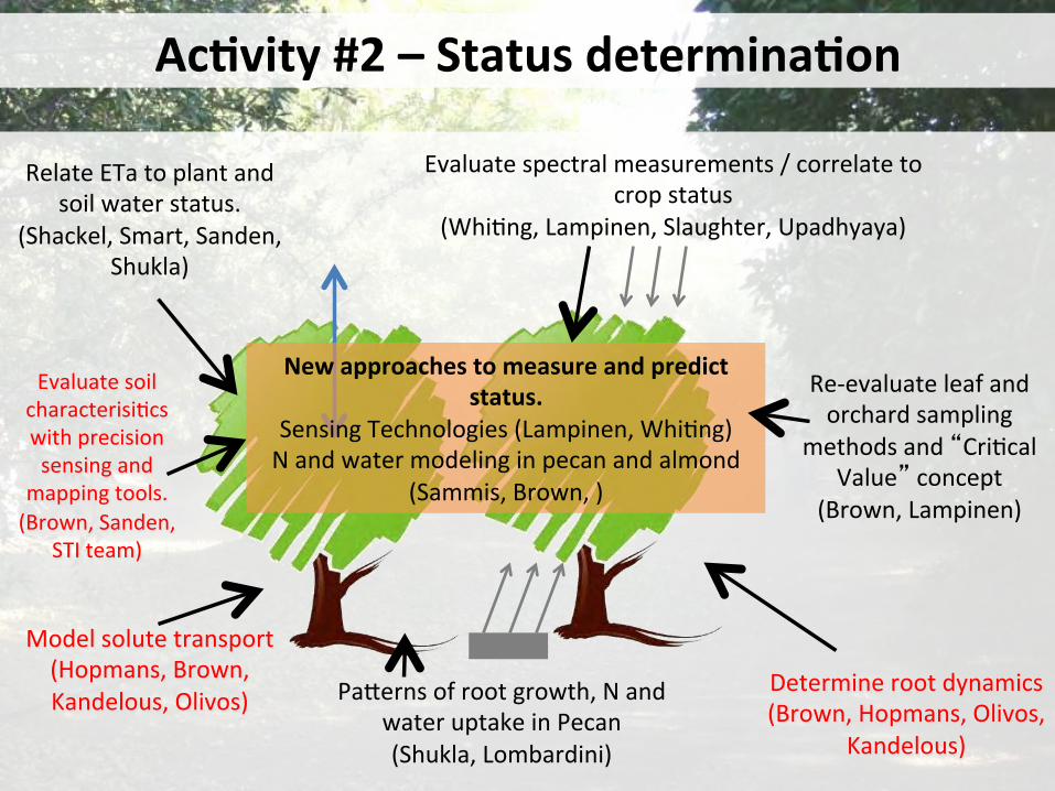
Ac#vity #2 – Status determina#on

Re-‐evaluate leaf and orchard sampling

methods and “CriFcal Value” concept

(Brown, Lampinen)

Relate ETa to plant and soil water status.

(Shackel, Smart, Sanden, Shukla)

Evaluate spectral measurements / correlate to crop status

(WhiFng, Lampinen, Slaughter, Upadhyaya)

New approaches to measure and predict status.

Sensing Technologies (Lampinen, WhiFng) N and water modeling in pecan and almond

(Sammis, Brown, )

Model solute transport (Hopmans, Brown, Kandelous, Olivos)

Determine root dynamics (Brown, Hopmans, Olivos,

Kandelous)

PaVerns of root growth, N and water uptake in Pecan (Shukla, Lombardini)

Evaluate soil characterisiFcs with precision sensing and

mapping tools. (Brown, Sanden,

STI team)

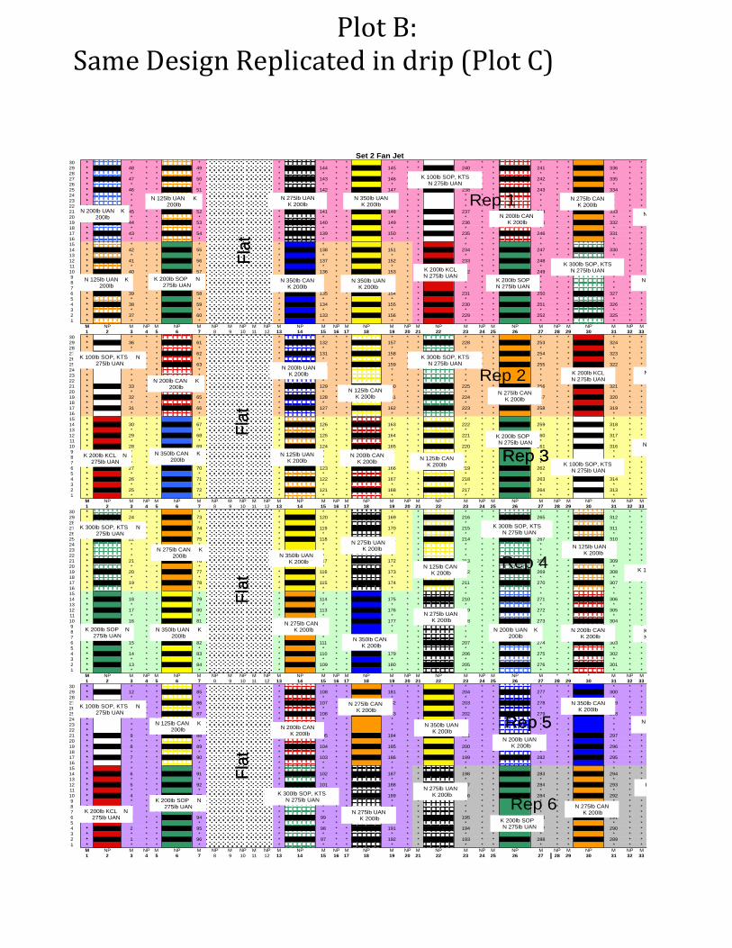
Two Replicated Trials (A-‐2011; B&C-‐2008)

Paramount-‐Belridge. 10 yo 50/50 NP:Monterey

C: N and K Rate and Source-Drip

B: N and K Rate and Source: FJ

A:Fertigation Method/K source

RCBD: 15 tree plots with 6 replicate plots per treatment. 12

treatments. Individual tree (768 NP)

monitoring.

RCBD: 15 tree plots with 5

replicate plots per treatment. 7 treatments.

Individual tree (NP and M) monitoring.

You are Here

30 * * * * * * * * * * * * * * * * * * * * *29 * 48 * * 49 * 144 * * 145 * * 240 * * 241 * * 336 * *28 * * * * * * * * * * * * * * * * * * * * *27 * 47 * * 50 * 143 * * 146 * * 239 * * 242 * * 335 * *26 * * * * * * * * * * * * * * * * * * * * *25 * 46 * * 51 * 142 * * 147 * * 238 * * 243 * * 334 * *24 * * * * * * * * * * * * * * * * * * * * *23 * * * * * * * * * * * * * * * * * * * * *22 * * * * * * * * * * * * * * * * * * * * *21 * 45 * * 52 * 141 * * 148 * * 237 * * 244 * * 333 * *20 * * * * * * * * * * * * * * * * * * * * *19 * 44 * * 53 * 140 * * 149 * * 236 * * 245 * * 332 * *18 * * * * * * * * * * * * * * * * * * * * *17 * 43 * * 54 * 139 * * 150 * * 235 * * 246 * * 331 * *16 * * * * * * * * * * * * * * * * * * * * *15 * * * * * * * * * * * * * * * * * * * * *14 * 42 * * 55 * 138 * * 151 * * 234 * * 247 * * 330 * *13 * * * * * * * * * * * * * * * * * * * * *12 * 41 * * 56 * 137 * * 152 * * 233 * * 248 * * 329 * *11 * * * * * * * * * * * * * * * * * * * * *10 * 40 * * 57 * 136 * * 153 * * 232 * * 249 * * 328 * *9 * * * * * * * * * * * * * * * * * * * * *8 * * * * * * * * * * * * * * * * * * * * *7 * * * * * * * * * * * * * * * * * * * * *6 * 39 * * 58 * 135 * * 154 * * 231 * * 250 * * 327 * *5 * * * * * * * * * * * * * * * * * * * * *4 * 38 * * 59 * 134 * * 155 * * 230 * * 251 * * 326 * *3 * * * * * * * * * * * * * * * * * * * * *2 * 37 * * 60 * 133 * * 156 * * 229 * * 252 * * 325 * *1 * * * * * * * * * * * * * * * * * * * * *

M NP M NP M NP M NP M NP M NP M NP M NP M NP M NP M NP M NP M NP M NP M NP M NP M1 2 3 4 5 6 7 8 9 10 11 12 13 14 15 16 17 18 19 20 21 22 23 24 25 26 27 28 29 30 31 32 33

30 * * * * * * * * * * * * * * * * * * * * *29 * 36 * * 61 * 132 * * 157 * * 228 * * 253 * * 324 * *28 * * * * * * * * * * * * * * * * * * * * *27 * 35 * * 62 * 131 * * 158 * * 227 * * 254 * * 323 * *26 * * * * * * * * * * * * * * * * * * * * *25 * 34 * * 63 * 130 * * 159 * * 226 * * 255 * * 322 * *24 * * * * * * * * * * * * * * * * * * * * *23 * * * * * * * * * * * * * * * * * * * * *22 * * * * * * * * * * * * * * * * * * * * *21 * 33 * * 64 * 129 * * 160 * * 225 * * 256 * * 321 * *20 * * * * * * * * * * * * * * * * * * * * *19 * 32 * * 65 * 128 * * 161 * * 224 * * 257 * * 320 * *18 * * * * * * * * * * * * * * * * * * * * *17 * 31 * * 66 * 127 * * 162 * * 223 * * 258 * * 319 * *16 * * * * * * * * * * * * * * * * * * * * *15 * * * * * * * * * * * * * * * * * * * * *14 * 30 * * 67 * 126 * * 163 * * 222 * * 259 * * 318 * *13 * * * * * * * * * * * * * * * * * * * * *12 * 29 * * 68 * 125 * * 164 * * 221 * * 260 * * 317 * *11 * * * * * * * * * * * * * * * * * * * * *10 * 28 * * 69 * 124 * * 165 * * 220 * * 261 * * 316 * *9 * * * * * * * * * * * * * * * * * * * * *8 * * * * * * * * * * * * * * * * * * * * *7 * * * * * * * * * * * * * * * * * * * * *6 * 27 * * 70 * 123 * * 166 * * 219 * * 262 * * 315 * *5 * * * * * * * * * * * * * * * * * * * * *4 * 26 * * 71 * 122 * * 167 * * 218 * * 263 * * 314 * *3 * * * * * * * * * * * * * * * * * * * * *2 * 25 * * 72 * 121 * * 168 * * 217 * * 264 * * 313 * *1 * * * * * * * * * * * * * * * * * * * * *


30 * * * * * * * * * * * * * * * * * * * * *29 * 24 * * 73 * 120 * * 169 * * 216 * * 265 * * 312 * *28 * * * * * * * * * * * * * * * * * * * * *27 * 23 * * 74 * 119 * * 170 * * 215 * * 266 * * 311 * *26 * * * * * * * * * * * * * * * * * * * * *25 * 22 * * 75 * 118 * * 171 * * 214 * * 267 * * 310 * *24 * * * * * * * * * * * * * * * * * * * * *23 * * * * * * * * * * * * * * * * * * * * *22 * * * * * * * * * * * * * * * * * * * * *21 * 21 * * 76 * 117 * * 172 * * 213 * * 268 * * 309 * *20 * * * * * * * * * * * * * * * * * * * * *19 * 20 * * 77 * 116 * * 173 * * 212 * * 269 * * 308 * *18 * * * * * * * * * * * * * * * * * * * * *17 * 19 * * 78 * 115 * * 174 * * 211 * * 270 * * 307 * *16 * * * * * * * * * * * * * * * * * * * * *15 * * * * * * * * * * * * * * * * * * * * *14 * 18 * * 79 * 114 * * 175 * * 210 * * 271 * * 306 * *13 * * * * * * * * * * * * * * * * * * * * *12 * 17 * * 80 * 113 * * 176 * * 209 * * 272 * * 305 * *11 * * * * * * * * * * * * * * * * * * * * *10 * 16 * * 81 * 112 * * 177 * * 208 * * 273 * * 304 * *9 * * * * * * * * * * * * * * * * * * * * *8 * * * * * * * * * * * * * * * * * * * * *7 * * * * * * * * * * * * * * * * * * * * *6 * 15 * * 82 * 111 * * 178 * * 207 * * 274 * * 303 * *5 * * * * * * * * * * * * * * * * * * * * *4 * 14 * * 83 * 110 * * 179 * * 206 * * 275 * * 302 * *3 * * * * * * * * * * * * * * * * * * * * *2 * 13 * * 84 * 109 * * 180 * * 205 * * 276 * * 301 * *1 * * * * * * * * * * * * * * * * * * * * *

M NP M NP M NP M NP M NP M NP M NP M NP M NP M NP M NP M NP M NP M * * * M NP M1 2 3 4 5 6 7 8 9 10 11 12 13 14 15 16 17 18 19 20 21 22 23 24 25 26 27 28 29 30 31 32 33

30 * * * * * * * * * * * * * * * * * * * * *29 * 12 * * 85 * 108 * * 181 * * 204 * * 277 * * 300 * *28 * * * * * * * * * * * * * * * * * * * * *27 * 11 * * 86 * 107 * * 182 * * 203 * * 278 * * 299 * *26 * * * * * * * * * * * * * * * * * * * * *25 * 10 * * 87 * 106 * * 183 * * 202 * * 279 * * 298 * *24 * * * * * * * * * * * * * * * * * * * * *23 * * * * * * * * * * * * * * * * * * * * *22 * * * * * * * * * * * * * * * * * * * * *21 * 9 * * 88 * 105 * * 184 * * 201 * * 280 * * 297 * *20 * * * * * * * * * * * * * * * * * * * * *19 * 8 * * 89 * 104 * * 185 * * 200 * * 281 * * 296 * *18 * * * * * * * * * * * * * * * * * * * * *17 * 7 * * 90 * 103 * * 186 * * 199 * * 282 * * 295 * *16 * * * * * * * * * * * * * * * * * * * * *15 * * * * * * * * * * * * * * * * * * * * *14 * 6 * * 91 * 102 * * 187 * * 198 * * 283 * * 294 * *13 * * * * * * * * * * * * * * * * * * * * *12 * 5 * * 92 * 101 * * 188 * * 197 * * 284 * * 293 * *11 * * * * * * * * * * * * * * * * * * * * *10 * 4 * * 93 * 100 * * 189 * * 196 * * 284 * * 292 * *9 * * * * * * * * * * * * * * * * * * * * *8 * * * * * * * * * * * * * * * * * * * * *7 * * * * * * * * * * * * * * * * * * * * *6 * 3 * * 94 * 99 * * 190 * * 195 * * 286 * * 291 * *5 * * * * * * * * * * * * * * * * * * * * *4 * 2 * * 95 * 98 * * 191 * * 194 * * 287 * * 290 * *3 * * * * * * * * * * * * * * * * * * * * *2 * 1 * * 96 * 97 * * 192 * * 193 * * 288 * * 289 * *1 * * * * * * * * * * * * * * * * * * * * *


Set 2 Fan Jet

Flat

Fl

at

Flat

Fl

at

Rep 3

Rep 4

Rep 5

Rep 2

Flat

Fl

at

Flat

Fl

at

Rep 1

Rep 3

Rep 5

Rep 6

N 200lb UAN K 200lb

N 350lb UAN K 200lb

N 350lb CAN K 200lb

K 200lb SOP N 275lb UAN

N 125lb UAN K 200lb

N 125lb UAN K 200lb

N 275lb UAN K 200lb

N 350lb UAN K 200lb

N 200lb CAN K 200lb

N 275lb CAN K 200lb

N 350lb CAN

N 125lb CAN K 200lb

N 275lb CAN K 200lb

N 275lb UAN

N 125lb CAN

N 125lb CAN K 200lb

N 125lb UAN K 200lb

N 350lb CAN K 200lb

N 200lb CAN K 200lb

N 125lb UAN K 200lb

N 200lb CAN K 200lb N 125lb CAN

K 200lb

N 200lb UAN

N 200lb UAN K 200lb

N 275lb CAN K 200lb N 350lb UAN

K 200lb

N 275lb UAN K 200lb

N 275lb UAN K 200lb

N 200lb UAN K 200lb

N 200lb CAN K 200lb

N 125lb CAN K 200lb N 200lb CAN

K 200lb

N 275lb CAN K 200lb

N 350lb UAN K 200lb

N 200lb UAN K 200lb

N 350lb CAN K 200lb

N 125lb UAN K 200lb

N 350lb UAN K 200lb

N 275lb CAN K 200lb

N 350lb CAN K 200lb

N 275lb UAN K 200lb

N 275lb UAN K 200lb

N 275lb CAN K 200lb






K 200lb KCL N 275lb UAN






K 100lb SOP, KTS N 275lb UAN










Plot B: Same Design Replicated in drip (Plot C)

Project Summary: It has been several decades since the last in-‐depth integrated analysis of almond

fertilization and irrigation and during this time the almond industry has seen tremendous growth in

production area, significant yield increases and a growing interest in environmental stewardship and

sustainability. As the industry grows and changes there is a need to continually improve the efficiency of

management of irrigation and fertilization so that economic and environmental sustainability can be

maintained. To optimize the use of irrigation and fertilizers requires 1) an ability to accurately measure and

estimate the amount and timing of nutrient and water demanded by the crop, 2) an understanding of the

interactions between fertilizer rate, fertilizer source, and application technique 3) an understanding of plant

response to irrigation deficit and excess, 4) an understanding of the basic biology of the tree, specifically the

patterns of root growth, nutrient uptake and plant demand, 5) an ability to monitor the movement and

minimize the losses of nitrogen and water from the system.

The projects you are visiting today are part of a large collaborative effort designed to address each of

these questions and to provide growers, consultants, regulators and educators the tools they need to ensure

that the Californian almond industry remains profitable, efficient and sustainable.

SEVEN STATIONS REPRESENTING 12 PROJECTS WILL BE PRESENTED

Start At The Station Number You Are Handed as You leave the Tent And

Proceed To The Next Highest Station Every 19 Minutes.

4 Stations Then Coffee: 3 Stations Then Lunch

1. Water use (ET) & plant stress guidelines – Blake Sanden (Kern UCCE), Ken Shackel, UCD

2. Learn to use the pressure chamber, hands on exercise – DeeAnn Kroeker, Kern UCCE

3. Nutrient budgets, fertilizer types and rate responses – Patrick Brown, Saiful Muhammad, UCD

4. Early season sampling and new critical values – Brown, Sebastian Saa Silva, UCD

5. Spur development, light and canopy potential – Bruce Lampinen, UCCE Davis

6. Remote sensing and spectral imagery as future tools – Mike Whiting, Susan Ustin, UCD

7. Nitrogen management & fate: Greenhouse gases, root distribution and irrigation impacts – Dave Smart, Daniel Schellenberg, Andres Olivos, UCD

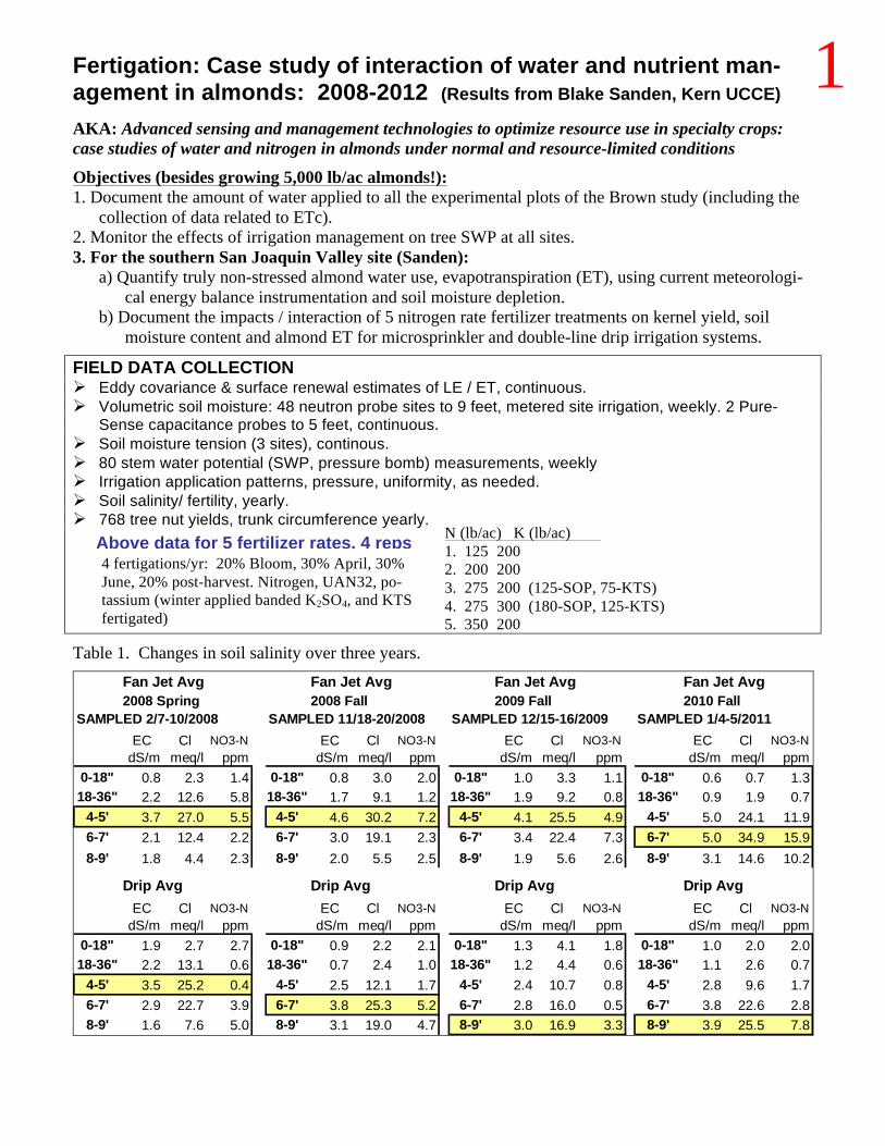
Fertigation: Case study of interaction of water and nutrient man-agement in almonds: 2008-2012 (Results from Blake Sanden, Kern UCCE) AKA: Advanced sensing and management technologies to optimize resource use in specialty crops: case studies of water and nitrogen in almonds under normal and resource-limited conditions Objectives (besides growing 5,000 lb/ac almonds!): 1. Document the amount of water applied to all the experimental plots of the Brown study (including the

collection of data related to ETc). 2. Monitor the effects of irrigation management on tree SWP at all sites. 3. For the southern San Joaquin Valley site (Sanden):

a) Quantify truly non-stressed almond water use, evapotranspiration (ET), using current meteorologi-cal energy balance instrumentation and soil moisture depletion.

b) Document the impacts / interaction of 5 nitrogen rate fertilizer treatments on kernel yield, soil moisture content and almond ET for microsprinkler and double-line drip irrigation systems.

FIELD DATA COLLECTION Ø Eddy covariance & surface renewal estimates of LE / ET, continuous. Ø Volumetric soil moisture: 48 neutron probe sites to 9 feet, metered site irrigation, weekly. 2 Pure-

Sense capacitance probes to 5 feet, continuous. Ø Soil moisture tension (3 sites), continous. Ø 80 stem water potential (SWP, pressure bomb) measurements, weekly Ø Irrigation application patterns, pressure, uniformity, as needed. Ø Soil salinity/ fertility, yearly. Ø 768 tree nut yields, trunk circumference yearly.

Table 1. Changes in soil salinity over three years.

Fan Jet Avg Fan Jet Avg Fan Jet Avg Fan Jet Avg2008 Spring 2008 Fall 2009 Fall 2010 Fall

SAMPLED 2/7-10/2008 SAMPLED 11/18-20/2008 SAMPLED 12/15-16/2009 SAMPLED 1/4-5/2011EC Cl NO3-N EC Cl NO3-N EC Cl NO3-N EC Cl NO3-N

dS/m meq/l ppm dS/m meq/l ppm dS/m meq/l ppm dS/m meq/l ppm0-18" 0.8 2.3 1.4 0-18" 0.8 3.0 2.0 0-18" 1.0 3.3 1.1 0-18" 0.6 0.7 1.318-36" 2.2 12.6 5.8 18-36" 1.7 9.1 1.2 18-36" 1.9 9.2 0.8 18-36" 0.9 1.9 0.7

4-5' 3.7 27.0 5.5 4-5' 4.6 30.2 7.2 4-5' 4.1 25.5 4.9 4-5' 5.0 24.1 11.96-7' 2.1 12.4 2.2 6-7' 3.0 19.1 2.3 6-7' 3.4 22.4 7.3 6-7' 5.0 34.9 15.98-9' 1.8 4.4 2.3 8-9' 2.0 5.5 2.5 8-9' 1.9 5.6 2.6 8-9' 3.1 14.6 10.2

Drip Avg Drip Avg Drip Avg Drip AvgEC Cl NO3-N EC Cl NO3-N EC Cl NO3-N EC Cl NO3-N

dS/m meq/l ppm dS/m meq/l ppm dS/m meq/l ppm dS/m meq/l ppm0-18" 1.9 2.7 2.7 0-18" 0.9 2.2 2.1 0-18" 1.3 4.1 1.8 0-18" 1.0 2.0 2.018-36" 2.2 13.1 0.6 18-36" 0.7 2.4 1.0 18-36" 1.2 4.4 0.6 18-36" 1.1 2.6 0.7

4-5' 3.5 25.2 0.4 4-5' 2.5 12.1 1.7 4-5' 2.4 10.7 0.8 4-5' 2.8 9.6 1.76-7' 2.9 22.7 3.9 6-7' 3.8 25.3 5.2 6-7' 2.8 16.0 0.5 6-7' 3.8 22.6 2.88-9' 1.6 7.6 5.0 8-9' 3.1 19.0 4.7 8-9' 3.0 16.9 3.3 8-9' 3.9 25.5 7.8

4 fertigations/yr: 20% Bloom, 30% April, 30% June, 20% post-harvest. Nitrogen, UAN32, po-tassium (winter applied banded K2SO4, and KTS fertigated)

Above data for 5 fertilizer rates, 4 reps N (lb/ac) K (lb/ac) 1. 125 200 2. 200 200 3. 275 200 (125-SOP, 75-KTS) 4. 275 300 (180-SOP, 125-KTS) 5. 350 200

1

Actual almond crop ET (as measured using eddy covariance heat flux) proved highly variable in the winter, early spring and fall of each season when compared to the Belridge CIMIS estimate of standard grass ET (ETo). Dividing the crop ET by ETo gives a crop coefficient value (Kc) that is assumed to be similar for all plantings of that crop in a like climate zone. The three years of Kc values for the fertigation trial are plotted below (Fig. 1). Large swings in Kc from 0.4 to 1.4 occur during the cool season because

ETo may be only 0.01 to 0.06”/day, but note that from mid May to mid August (Non-pariel harvest) all years have good agreement with Kc values running from 1.0 to 1.2. ETo can reach 0.30” during this time with measured almond ET as high as 0.35”/day.

Figure 2 compares 3 almond Kc curves on a biweekly basis. The lower one is the old UC almond curve from the 1960’s, with a Kern County “normal year” ET of 42 inches with a peak Kc of 0.95. The next curve is the Sanden model estimate from irrigation monitoring demonstrations in more than 50 almond blocks over 12 years at 52 inches and a peak Kc of 1.08. The top curve is not as smooth because it uses

the actual measured aver-age Kc values from March 2008 through December 2010 (Fig.1), for a final “normal year” ET of 60 inches and a peak Kc of 1.19. The or-chard is irrigat-ed with 2, A-40 Bowsmith Fan-jets per tree (21x24 foot spacing) planted as alternating Nonpareil and

Monterey. Note the dip in the Kc value for the end of August from harvest irrigation cutoff stress.

0.0

0.2

0.4

0.6

0.8

1.0

1.2

1.4

Jan Feb Mar Apr May Jun Jul Aug Sep Oct Nov Dec

Bi-w

eekl

y Al

mon

d Cr

op C

oeffi

cien

t (Kc

)

Older Published KcSanden SSJV Kc2008 - 10 Measd Kc

Avg Kc 4/1 - 11/15 Calculated Avg ET Older Avg Kc = 0.81 42.2 in (4/1 - 11/15) Sanden Avg Kc = 0.93 52.3 in (year)Measured Avg Kc = 1.05 60.4 in (year)

(Using CIMIS Zone 15 "Historic Eto" = 57.9 in)

Comparison of “old” almond crop Kc values and Kern data

0.00

0.20

0.40

0.60

0.80

1.00

1.20

1.40

1/1 1/29 2/26 3/26 4/23 5/21 6/18 7/16 8/13 9/10 10/8 11/5 12/3 12/31Wee

kly

Mea

sure

d Ed

dy C

ovar

ianc

e Cr

op C

oeffi

cien

t (Kc

)

2008: 52.8 in2009: 61.5 in2010: 54.9 in

Comparison of 3 years of mature almond crop coefficients geneed from EDDY COVARIANCE heat flux estimates of crop ET divided by the modified Penman ETo from the Belridge CIMIS station #146 1.5 miles due west of orchard. (2008 ET measured 3/19to 11/11. 2009 and 2010 are full year.)

Weekly crop coefficient values (Kc) for 2008-2010

Fig. 2 Biweekly almond crop coefficient curves.

Fig. 1 Weekly Kc values for all years

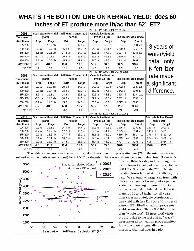
WHAT’S THE BOTTOM LINE ON KERNAL YIELD: does 60 inches of ET produce more lb/ac than 52” ET?

(NP ET for 2008 is for 2/7 to 11/17)2008

Treatment(N-K lb/ac)

125-200 -- -10.2 ab -- 12.6 a -- 55.3 a -- 3301 ab200-200 -9.6 a -9.7 b 16.8 a 14.9 b 54.5 a 56.1 a 3260 a 3360 b275-200 -8.5 ab -10.1 ab 17.4 ab 14.7 ab 57.3 a 57.7 a 3997 b 3338 ab275-300 -8.4 b -10.3 a 16.8 b 12.9 ab 55.9 a 55.3 a 3839 ab 3370 a350-200 -9.5 ab -10.0 ab 15.4 ab 13.9 ab 56.2 a 55.6 a 3518 ab 3963 ab

AVERAGE -9.0 -10.0 16.6 13.8 55.9 56.0 3653 3467LSD 0.05 1.1 0.6 2.3 2.3 4.8 2.5 715 517

(NP ET for 2009 is for 1/27 to 12/2)2009


125-200 -9.6 a -10.5 ab 18.0 a 14.2 a 54.9 a 56.9 a 2722 a 3027 ab200-200 -9.3 ab -10.4 b 18.2 a 17.1 b 58.2 a 57.6 a 2642 a 3005 a275-200 -8.9 b -11.1 a 18.8 a 15.8 ab 60.5 a 58.3 a 3524 b 3164 abc275-300 -8.3 c -11.0 ab 18.6 a 14.2 a 59.2 a 57.0 a 3572 b 3783 c350-200 -9.7 a -11.0 ab 15.3 a 14.9 ab 58.3 a 56.5 a 3727 b 3858 bc

AVERAGE -9.2 -10.8 17.8 15.2 58.2 57.3 3237 3367LSD 0.05 0.6 0.7 6.2 2.7 6.9 3.5 752 844

(NP ET for 2010 is for 1/1 to 12/6 )2010


125-200 -9.8 a 11.1 a 15.9 ab 14.4 a 56.8 a 55.5 a 3565 a 3280 a 2865 a 2909 a200-200 -9.7 a 11.9 b 17.2 b 15.1 a 57.0 a 54.4 a 3779 ab 3591 ab 3453 b 3405 b275-200 -9.7 a 12.5 b 17.7 b 16.2 a 56.6 a 55.0 a 4266 bc 3914 bc 3765 bc 3813 bc275-300 -10.1 a 12.1 b 16.7 ab 14.5 a 57.5 a 55.1 a 4069 cd 3804 bc 3844 bc 3806 bc350-200 -9.7 a 11.9 b 14.6 a 15.3 a 56.4 a 55.0 a 4717 d 4165 c 4064 c 3924 c

AVERAGE -9.8 11.9 16.4 15.1 56.9 55.0 4079 3751 3598 3571LSD 0.05 0.5 0.6 2.5 2.9 3.7 3.3 457 415

Trial Whole Plot Kernal Yield (lb/ac)

Drip Fanjet

Drip Fanjet Drip Fanjet

Stem Water Potential (bars)

Soil Water Content to 9 feet (in)

Cumulative Neutron Probe ET (in) Final Kernal Yield (lb/ac)




Drip Fanjet

Drip FanjetDrip Fanjet

Drip Fanjet




Drip Fanjet Drip Fanjet

FanjetDrip Fanjet Drip Fanjet Drip Fanjet Drip

3 years of water/yield data: only N fertilizer rate made

a significant difference.

The table above describes the results from 40 different neutron probe site trees (20 in the micro-sprinkler set and 20 in the double-line drip set) for UAN32 treatments. There is no difference in individual tree ET due to N.

The 125 lb/ac N rate produced a signifi-cantly lower kernel yield compared to the 350 lb/ac N rate with the 275 lb N rate trending lower but not statistically signifi-cant. We attempt to irrigate all trees with the same amount of water, but irrigation system and tree vigor non-uniformity produced annual individual tree ET esti-mates of 51 to 63 inches for all years. There was absolutely no correlation of tree yield with tree ET above 51 inches of almond ET. Finally, neutron probe tree yields were about 200 to 600 lb/ac higher than “whole plot” (15 trees/plot) yields – probably due to the fact that no “weak” trees are used for neutron probe monitor-ing while there is generally one or moreweak/barked trees in a plot.

1500

2000

2500

3000

3500

4000

4500

5000

5500

50 52 54 56 58 60 62 64Season-Long Soil Water Depletion ET (in)

Ker

nal Y

ield

(lb/

ac)

200820092010

Fig. 3. Correlation of indi-vidual tree ET & yield

Can we manage irrigation from outer space by measuring ET? Ken Shackel, Blake Sanden, Rick Snyder, Ted Sammis, Sam Prentice, Gerardo Spinelli

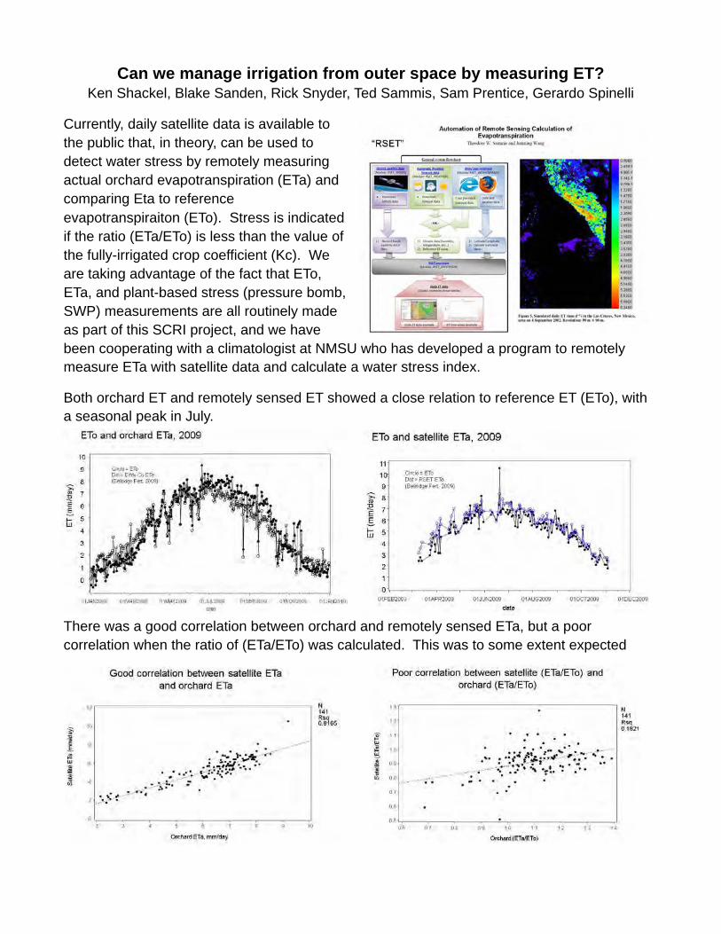
Currently, daily satellite data is available to the public that, in theory, can be used to detect water stress by remotely measuring actual orchard evapotranspiration (ETa) and comparing Eta to reference evapotranspiraiton (ETo). Stress is indicated if the ratio (ETa/ETo) is less than the value of the fully-irrigated crop coefficient (Kc). We are taking advantage of the fact that ETo, ETa, and plant-based stress (pressure bomb, SWP) measurements are all routinely made as part of this SCRI project, and we have been cooperating with a climatologist at NMSU who has developed a program to remotely measure ETa with satellite data and calculate a water stress index.

Both orchard ET and remotely sensed ET showed a close relation to reference ET (ETo), with a seasonal peak in July.

There was a good correlation between orchard and remotely sensed ETa, but a poor correlation when the ratio of (ETa/ETo) was calculated. This was to some extent expected

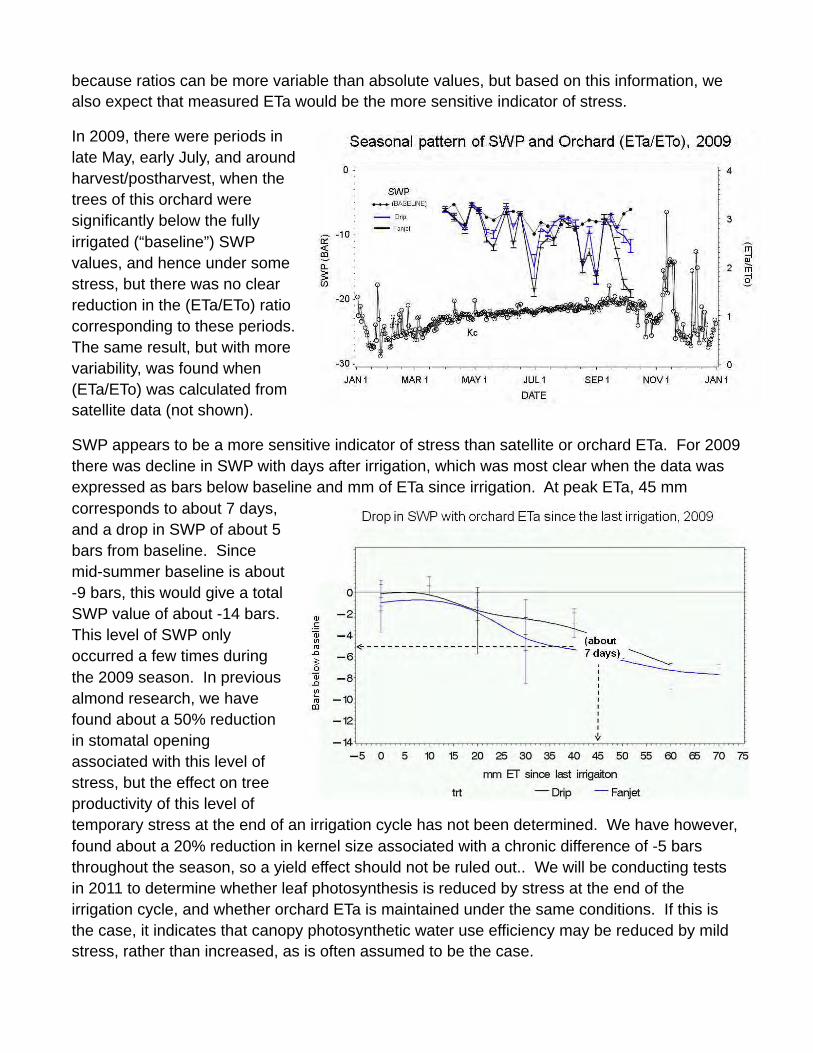
because ratios can be more variable than absolute values, but based on this information, we also expect that measured ETa would be the more sensitive indicator of stress.

In 2009, there were periods in late May, early July, and around harvest/postharvest, when the trees of this orchard were significantly below the fully irrigated (“baseline”) SWP values, and hence under some stress, but there was no clear reduction in the (ETa/ETo) ratio corresponding to these periods. The same result, but with more variability, was found when (ETa/ETo) was calculated from satellite data (not shown).

SWP appears to be a more sensitive indicator of stress than satellite or orchard ETa. For 2009 there was decline in SWP with days after irrigation, which was most clear when the data was expressed as bars below baseline and mm of ETa since irrigation. At peak ETa, 45 mm corresponds to about 7 days, and a drop in SWP of about 5 bars from baseline. Since mid-summer baseline is about -9 bars, this would give a total SWP value of about -14 bars. This level of SWP only occurred a few times during the 2009 season. In previous almond research, we have found about a 50% reduction in stomatal opening associated with this level of stress, but the effect on tree productivity of this level of temporary stress at the end of an irrigation cycle has not been determined. We have however, found about a 20% reduction in kernel size associated with a chronic difference of -5 bars throughout the season, so a yield effect should not be ruled out.. We will be conducting tests in 2011 to determine whether leaf photosynthesis is reduced by stress at the end of the irrigation cycle, and whether orchard ETa is maintained under the same conditions. If this is the case, it indicates that canopy photosynthetic water use efficiency may be reduced by mild stress, rather than increased, as is often assumed to be the case.

Nutrient Budget approach to Nutrient Management in Almond Saiful Muhammad and Patrick H. Brown

Plant Sciences, University of California-‐Davis [email protected]

Background: In Almond and most fruit trees nutrient management has been based on leaf sampling and critical values. The critical value is the nutrient concentration in a standard leaf sample at a specific time in the season above which no further response to nutrient addition can be expected. Critical values are ideally developed on the basis of careful experimentation where the relationship between yield and nutrient concentration is closely monitored. While leaf analysis is useful to identify nutrient deficiencies and to provide an ongoing record of crop response, the methodology has some limitations:

• While leaf analysis can be used to monitor changes over time and identify If a particular nutrient is deficient, it cannot provide information on how much nutrient is required by the crop.

• Leaf tissue analysis is expensive and slow and often difficult to interpret.

• Leaf tissue analysis is reactive and cannot be used to predict nutrient demand or schedule fertilizations.

Approach: Development Of A Nutrient Budget Approach To Fertilizer Management. In many high value crops nutrient budgets have been developed in which nutrient demand for a given crop yield are determined and used to estimate fertilization rates. This approach is based upon the premise that a given yield removes a specific quantitiy of nutrient from the field and that fertilization should aim to replace that removal with as great an efficiency as possible. This experiment aims to develop a nutrient budget for almond based on the expected yield and tree phenology and to determine the effect of different nitrogen and potassium rates and sources on tissue nutrient, yield and nutrient export from the orchard. Experimental Design (Table 1): The experiment has been set up under fan Jet and drip irrigations. There are four nitrogen rates ‘125, 200, 275 and 350lb/ac’ nitrogen and two sources of nitrogen as Urea Ammonium Nitrate 32 (UAN 32) and Calcium Ammonium Nitrate 17 (CAN 17). Three potassium rates ‘100, 200 and 300lb/ac’ and three potassium sources ‘Sulphate of Potash (SOP)’, ‘60% SOP+40% Potassium Thiosulfate (KTS)’ and ‘Potassium Chloride (KCl)’. The entire SOP applied as granular in December-‐January and the remaining potassium and all nitrogen fertigated in four fertigation cycles in February (before bloom), early April, mid June and after harvest in September-‐October at 20%, 30%, 30% and 20% respectively. Leaf samples were collected four times and fruit samples were collected five times during the season from 768 individual trees. Trees were individually harvested.

3

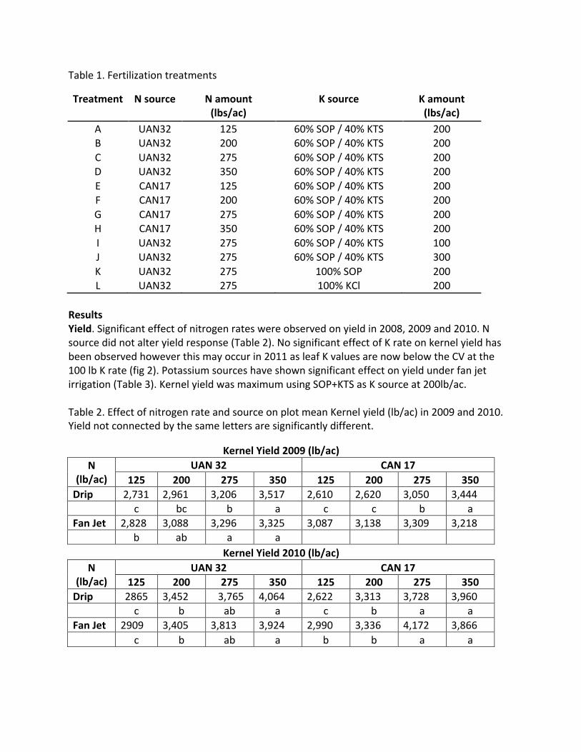
Table 1. Fertilization treatments

Treatment N source N amount (lbs/ac)

K source K amount (lbs/ac)

A UAN32 125 60% SOP / 40% KTS 200 B UAN32 200 60% SOP / 40% KTS 200 C UAN32 275 60% SOP / 40% KTS 200 D UAN32 350 60% SOP / 40% KTS 200 E CAN17 125 60% SOP / 40% KTS 200 F CAN17 200 60% SOP / 40% KTS 200 G CAN17 275 60% SOP / 40% KTS 200 H CAN17 350 60% SOP / 40% KTS 200 I UAN32 275 60% SOP / 40% KTS 100 J UAN32 275 60% SOP / 40% KTS 300 K UAN32 275 100% SOP 200 L UAN32 275 100% KCl 200

Results Yield. Significant effect of nitrogen rates were observed on yield in 2008, 2009 and 2010. N source did not alter yield response (Table 2). No significant effect of K rate on kernel yield has been observed however this may occur in 2011 as leaf K values are now below the CV at the 100 lb K rate (fig 2). Potassium sources have shown significant effect on yield under fan jet irrigation (Table 3). Kernel yield was maximum using SOP+KTS as K source at 200lb/ac. Table 2. Effect of nitrogen rate and source on plot mean Kernel yield (lb/ac) in 2009 and 2010. Yield not connected by the same letters are significantly different.

Kernel Yield 2009 (lb/ac) N

(lb/ac) UAN 32 CAN 17

125 200 275 350 125 200 275 350 Drip 2,731 2,961 3,206 3,517 2,610 2,620 3,050 3,444 c bc b a c c b a Fan Jet 2,828 3,088 3,296 3,325 3,087 3,138 3,309 3,218 b ab a a

Kernel Yield 2010 (lb/ac) N

(lb/ac) UAN 32 CAN 17

125 200 275 350 125 200 275 350 Drip 2865 3,452 3,765 4,064 2,622 3,313 3,728 3,960 c b ab a c b a a Fan Jet 2909 3,405 3,813 3,924 2,990 3,336 4,172 3,866 c b ab a b b a a

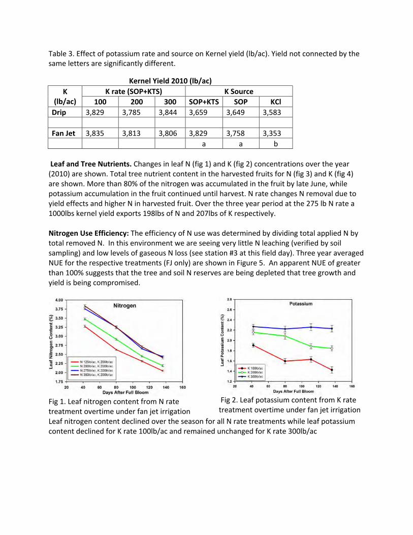
Table 3. Effect of potassium rate and source on Kernel yield (lb/ac). Yield not connected by the same letters are significantly different.

Kernel Yield 2010 (lb/ac) K

(lb/ac) K rate (SOP+KTS) K Source

100 200 300 SOP+KTS SOP KCl Drip 3,829 3,785 3,844 3,659 3,649 3,583 Fan Jet 3,835 3,813 3,806 3,829 3,758 3,353 a a b Leaf and Tree Nutrients. Changes in leaf N (fig 1) and K (fig 2) concentrations over the year (2010) are shown. Total tree nutrient content in the harvested fruits for N (fig 3) and K (fig 4) are shown. More than 80% of the nitrogen was accumulated in the fruit by late June, while potassium accumulation in the fruit continued until harvest. N rate changes N removal due to yield effects and higher N in harvested fruit. Over the three year period at the 275 lb N rate a 1000lbs kernel yield exports 198lbs of N and 207lbs of K respectively. Nitrogen Use Efficiency: The efficiency of N use was determined by dividing total applied N by total removed N. In this environment we are seeing very little N leaching (verified by soil sampling) and low levels of gaseous N loss (see station #3 at this field day). Three year averaged NUE for the respective treatments (FJ only) are shown in Figure 5. An apparent NUE of greater than 100% suggests that the tree and soil N reserves are being depleted that tree growth and yield is being compromised.

Fig 1. Leaf nitrogen content from N rate treatment overtime under fan jet irrigation

Fig 2. Leaf potassium content from K rate treatment overtime under fan jet irrigation

Leaf nitrogen content declined over the season for all N rate treatments while leaf potassium content declined for K rate 100lb/ac and remained unchanged for K rate 300lb/ac

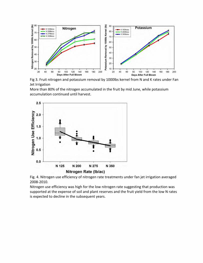
Fig 3. Fruit nitrogen and potassium removal by 1000lbs kernel from N and K rates under Fan Jet Irrigation More than 80% of the nitrogen accumulated in the fruit by mid June, while potassium accumulation continued until harvest.

Fig. 4. Nitrogen use efficiency of nitrogen rate treatments under fan jet irrigation averaged 2008-‐2010. Nitrogen use efficiency was high for the low nitrogen rate suggesting that production was supported at the expense of soil and plant reserves and the fruit yield from the low N rates is expected to decline in the subsequent years.

Leaf Nutrient Sampling Updates Sebastian Saa, Patrick Brown, Emilio Laca

Plant Sciences, University of California-‐Davis Contact: [email protected]

Preliminary Results: (this is year four of a five year project, the following guidelines may be amended as new results become available. We welcome your ideas and experiences.)

• New Guidelines For Early Season Leaf Nutrient Sampling For California Almond Orchards • New Approaches for Almond Tissue and Field Sampling • Evaluation and Improvement of Leaf Critical Values and Interpretation Guidelines.

Introduction: This research is based upon the results of a survey of almond growers and consultants in California conducted in 2007 that suggested that leaf sampling and comparison with established standards were not fully meeting grower needs. To address these concerns this current project is designed to provide new information on:

• Early season leaf analysis protocols and the relationship between current leaf sampling protocols, new leaf sampling protocols, and yield.

• The use of fruiting spur leaf analysis as a means to determine almond tree nutrient status, nutrient demand and possible response to fertilization.

• To characterize nutrient variability between months, years and within orchards so that tissue sampling can become more robust and interpretable.

Results & Conclusions:

• Fruiting spurs can exhibit nutrient deficiencies that can limit photosynthesis even when non-‐fruiting leaves on the same tree may have “adequate” leaf concentrations (Figure 1).

• This observation and statistical analysis suggest that fruiting spurs may be better indicators of tree-‐nutrient-‐status than non-‐fruiting spurs.

• Some existing critical values may be incorrect (like S), others appear to be correct (N) and some remain uncertain (K).

• July-‐nitrogen-‐content (and likely other nutrients) can be well predicted with an early (April) sampling (figure 2).

• April leaf sampling can be used to effectively predict the percentage of trees that will be nitrogen limited in July (figure 2).

• Variability of nitrogen and other elements within four orchards over 4 years has been characterized and used to determine how many tissue samples must be collected to reliably determine orchard nutrient status.

o It is feasible to sample orchards for N status and to use that value to prescribe management.

o However, for some nutrients (K and Mn) it is NOT feasible to sample orchards for nutrient status and to use that value to prescribe management except when trees are exhibiting clear deficiency (Figure 3).

4

Take Home Message:

• A new protocol based on sampling leaves from fruiting spurs during April-‐May will be finalized in 2011 and made available to growers in 2012.

• For those wishing to pre-‐validate this approach you should collect April samples from leaves of fruiting spurs and include analysis of eleven essential elements (N-‐P-‐K-‐B-‐Zn-‐Ca-‐Mn-‐Mg-‐Fe-‐S-‐Cu).

o This approach can then be used to provide your own correlation with July nitrogen content. Sharing these results with us ([email protected]) will strengthen our model development.

• To obtain a meaningful estimate of average orchard leaf nitrogen concentrations using current methodology, at least 4 independent samples should be collected from each orchard (4 samples taken from discrete trees or groups of trees and analyzed separately). The average of these 4 trees can then be used to determine field N status.

• In most moderately uniform orchards, our multi-‐site and multi-‐year analysis demonstrates that a July leaf nitrogen value of 2.4% in non fruiting leaves indicates that 95% of all trees in your orchard are above the critical value (CV), while a July leaf N value of 2.3% in non fruiting leaves suggests that 85% of all trees will be above the critical value (CV).

o Please Note: A tree that is below the critical value of 2.2% has the potential for reduced yield however the extent of that lost yield is not yet quantified.

• July leaf analysis for K and Mn provide little useful information except when clearly deficient. Further analysis of this problem is underway.

Selected Results:

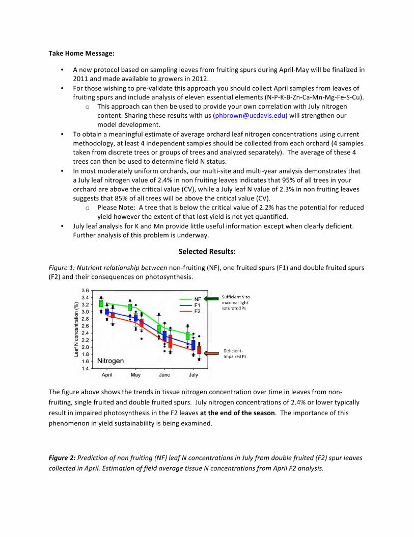
Figure 1: Nutrient relationship between non-‐fruiting (NF), one fruited spurs (F1) and double fruited spurs (F2) and their consequences on photosynthesis.

The figure above shows the trends in tissue nitrogen concentration over time in leaves from non-‐fruiting, single fruited and double fruited spurs. July nitrogen concentrations of 2.4% or lower typically result in impaired photosynthesis in the F2 leaves at the end of the season. The importance of this phenomenon in yield sustainability is being examined.

Figure 2: Prediction of non fruiting (NF) leaf N concentrations in July from double fruited (F2) spur leaves collected in April. Estimation of field average tissue N concentrations from April F2 analysis.

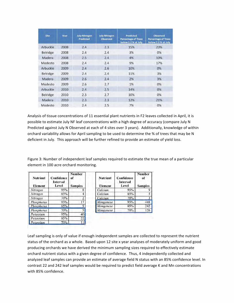
Analysis of tissue concentrations of 11 essential plant nutrients in F2 leaves collected in April, it is possible to estimate July NF leaf concentrations with a high degree of accuracy (compare July N Predicted against July N Observed at each of 4 sites over 3 years). Additionally, knowledge of within orchard variability allows for April sampling to be used to determine the % of trees that may be N deficient in July. This approach will be further refined to provide an estimate of yield loss.

Figure 3: Number of independent leaf samples required to estimate the true mean of a particular element in 100 acre orchard monitoring.

Leaf sampling is only of value if enough independent samples are collected to represent the nutrient status of the orchard as a whole. Based upon 12 site x year analyses of moderately uniform and good producing orchards we have derived the minimum sampling sizes required to effectively estimate orchard nutrient status with a given degree of confidence. Thus, 4 independently collected and analyzed leaf samples can provide an estimate of average field N status with an 85% confidence level. In contrast 22 and 242 leaf samples would be required to predict field average K and Mn concentrations with 85% confidence.

Infrared thermometers(soil surface temperature)

spring loadedsection

protective cage reference weatherstation

GPS

light bars

720 photodiodes active in PAR rangeSampling rate of 10Hz (cycles per second)Adjustable from ~8’ to 32’Driven at ~7 mphSub-‐meter GPS

UCCE/PFC Almond Fertility Field Day, June 16, 2011

Relationship Between Midday Canopy Light Interception and Yield Potential in Almond Bruce Lampinen, Integrated Management/Almond and Walnut Specialist, UC Davis

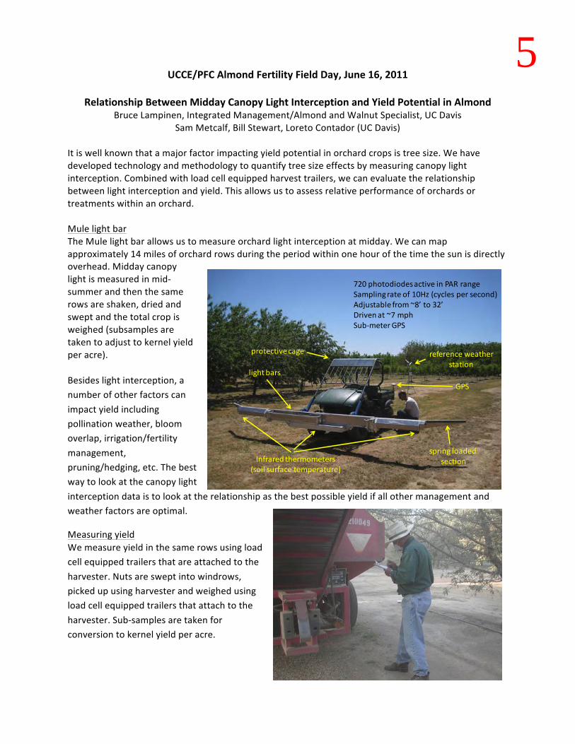
Sam Metcalf, Bill Stewart, Loreto Contador (UC Davis) It is well known that a major factor impacting yield potential in orchard crops is tree size. We have developed technology and methodology to quantify tree size effects by measuring canopy light interception. Combined with load cell equipped harvest trailers, we can evaluate the relationship between light interception and yield. This allows us to assess relative performance of orchards or treatments within an orchard. Mule light bar The Mule light bar allows us to measure orchard light interception at midday. We can map approximately 14 miles of orchard rows during the period within one hour of the time the sun is directly overhead. Midday canopy light is measured in mid-‐summer and then the same rows are shaken, dried and swept and the total crop is weighed (subsamples are taken to adjust to kernel yield per acre). Besides light interception, a number of other factors can impact yield including pollination weather, bloom overlap, irrigation/fertility management, pruning/hedging, etc. The best way to look at the canopy light interception data is to look at the relationship as the best possible yield if all other management and weather factors are optimal.

Measuring yield We measure yield in the same rows using load cell equipped trailers that are attached to the harvester. Nuts are swept into windrows, picked up using harvester and weighed using load cell equipped trailers that attach to the harvester. Sub-‐samples are taken for conversion to kernel yield per acre.

5

Hand light bar data 2000-2008 Mule light bar data 2009-2010

Midday light interception (%)

0 20 40 60 80 100

Ker

nel y

ield

(lbs

/acr

e)

0500

10001500200025003000350040004500500055006000

WalnutAlmond

Fig. 1. Midday photosynthetically active radiation(%) interception versus pounds per acre of kernel yield for almond and walnut data from various trials

3222 72

*pink and yellow dots in right hand graph indicate two year average yield and light interception for Nickels training/pruning trial (where we are standing) and for Nickels rootstock block (next block to the west) respectively

All almond light bar sites 2009 and 2010

Midday canopy PAR interception (%)0 20 40 60 80 100

Yiel

d (k

erne

l lbs/

ac)

0

1000

2000

3000

4000

5000

60002009 all data2010 all data2009 Belridge drip2009 Belridge fanjet2010 Belridge drip2010 Belridge fanjet

Relationship between midday canopy light interception and yield When light interception is plotted against yield, there appears to be an upper limit which is about 50 kernel pounds of almonds that can potentially be produced with each 1% of the total incoming light that is intercepted (Fig. 1). The maximum light interception is approximately 90-‐93% in a fully canopied orchard so maximum yield potential is about 4500 (90x50=4500) kernel pounds per acre for almond. This would assume all other factors are optimal including minimal/no pruning, optimal water/nutrition management, good bloom weather, good pollinizer bloom overlap, quality bee hives, etc.

Fig. 1. Midday canopy light interception/yield data

collected with a hand light bar (left) and with the Mule light bar (right). The large number of sites that were above optimal line in 2009 season (right hand graph above), were largely due to alternate bearing and these sites were lower in 2010 and/or in 2008. Data for Belridge SCRI orchard are shown in color.

Spur Dynamics We have not found orchards that can produce consistently above 4300 kernel pounds per acre or above 50 kernel pounds per 1% light intercepted. From data we have collected so far, an orchard that is above this level one year will be below this level the next year. At least part of the reason for this is that individual spurs alternate bear. If an orchard produces above 50 kernel pounds per 1% light intercepted, it likely means that more spurs were bearing than a tree can sustain from year to year. Therefore, in the following year, all of the spurs that bore fruit the previous year will be either dead or in a vegetative state and yield will be below 50 kernel pounds per 1% light intercepted.

Food safety related issues There are potential food safety related issues for orchards with very high midday canopy light interception. When midday canopy light interception increases above about 75% or so (yield potential of about 3800 kernel pounds per acre, food safety risk is likely increased due to cooler soil conditions that are conducive to Salmonella survival and also because the shaded conditions on the orchard floor make it more difficult to dry nuts at the time of harvest. Therefore, if your orchard has produced above 3800 kernel pounds per acre, you should pay particular attention to food safety risk. This would include making sure that nuts are adequately dry before they are picked up (particularly if they are going to be stockpiled) and that pathogens are not introduced inadvertently (i.e. with manure applications).

Hand light bar data 2001-‐2008 Mobile platform light bar data 2009-‐10

Remote sensing The canopy light interception data from the mobile platform light bar is being used to ground truth remotely sensed imagery collected by other colleagues involved in this project (see station #6-‐ Whiting/Ustin et.al.). Other uses of this technology This technology allows us to assess new varieties regarding their yield potential compared to existing varieties. In particular, we can identify whether a new variety is more productive per unit light intercepted or if it simply grows faster than existing varieties. It also allows pruning/hedging trials to be evaluated in terms of productivity per unit light intercepted. In addition, we can evaluate soil treatments (e.g. fumigation, soil amendments, etc.) to be evaluated as to their impacts on canopy growth versus direct effects on yield potential per unit light intercepted. Light interception/yield results from Belridge SCRI orchard Midday canopy light interception tended to increase with increasing nitrogen application rate in both years and in both drip and fanjet orchards (Fig. 2a, 2b). In the fanjet orchard, midday canopy light interception increased in all treatments from 2009 to 2010 (Fig. 2b). However, in the drip orchard, midday canopy light interception decreased in all treatments from 2009 to 2010 (Fig. 2a; except the high N level which stayed constant). It is unclear what caused this decrease. You would expect midday canopy light interception to be increasing from 2009 to 2010 since the orchard was mechanically hedged before the 2009 season. One potential explanation might be lower canopy leaf loss due to hull rot. We are assessing disease incidence in both orchards in 2011 to attempt to understand these results. Based on the light interception data from 2010, we would expect to see higher yields in the fanjet orchard compared to the drip orchard in 2011. The yields in the drip and fanjet orchards ranged from 3000 to 4200 kernel pounds per acre in 2010 which are very good yields (Fig. 2c, 2d). The yield per unit light intercepted reached the 50 kernel pounds per unit light intercepted level in 2010 which is the highest sustainable yield we might expect based on previous data (see diagonal line in Fig. 1).

Fig. 2. Midday canopy light interception for the drip, yield and yield per unit light intercepted for the drip and fanjet orchards.

Land, A ir and Water ResourcesDepartment of

University of California, DavisLand, A ir and Water ResourcesDepartment of

University of California, Davis

Center for Spatial Technologies and Remote Sensing

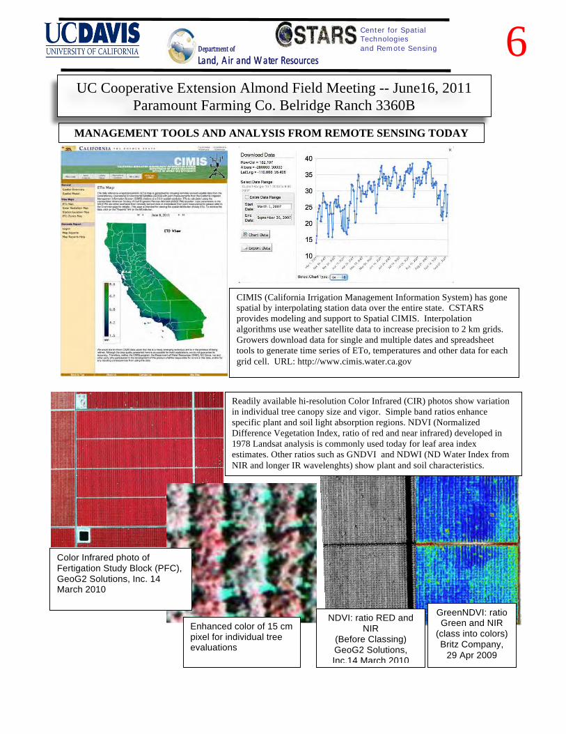
CIMIS (California Irrigation Management Information System) has gone spatial by interpolating station data over the entire state. CSTARS provides modeling and support to Spatial CIMIS. Interpolation algorithms use weather satellite data to increase precision to 2 km grids. Growers download data for single and multiple dates and spreadsheet tools to generate time series of ETo, temperatures and other data for each grid cell. URL: http://www.cimis.water.ca.gov

NDVI: ratio RED and NIR

(Before Classing) GeoG2 Solutions, Inc.14 March 2010

GreenNDVI: ratio Green and NIR

(class into colors) Britz Company,

29 Apr 2009

Enhanced color of 15 cm pixel for individual tree evaluations

Color Infrared photo of Fertigation Study Block (PFC), GeoG2 Solutions, Inc. 14 March 2010

Readily available hi-resolution Color Infrared (CIR) photos show variation in individual tree canopy size and vigor. Simple band ratios enhance specific plant and soil light absorption regions. NDVI (Normalized Difference Vegetation Index, ratio of red and near infrared) developed in 1978 Landsat analysis is commonly used today for leaf area index estimates. Other ratios such as GNDVI and NDWI (ND Water Index from NIR and longer IR wavelenghts) show plant and soil characteristics.

MANAGEMENT TOOLS AND ANALYSIS FROM REMOTE SENSING TODAY

UC Cooperative Extension Almond Field Meeting -- June16, 2011 Paramount Farming Co. Belridge Ranch 3360B

6

Contact: Mike Whiting ([email protected]) or Susan Ustin ([email protected]) CSTARS, LAWR, University of California, One Shields Ave., Davis, 95616

Every 16 days Landsat images provide same 30 m pixel areas for analyzing multiple seasons of canopy reflectance to relate variation to water and nutrient stress, and yield. Time series can also be created for CIMIS and other continuous environmental and farm management data to compare to images time series.

2007 2008 2009 2010 20 April

7 June 10 August

27 September

Landsat NDWI values for same pixel with fitted curve for analysis

Time Series analysis for understanding season to season variation

Interpolations vs. WRF Model for temperature

Improved Atmospheric Model: Forecast ETc at 1km high-resolution

National Atmospheric Research Center: WRF-ACASA models ETc with NWS

forecast to 5 days ahead.

01 June 2008 12:00PST, southern San Joaquin Valley model

(integrating landcover mapping) Red: High ETa in crop areas, Blue: Low ETa in dry range land

FUTURE MANAGEMENT TOOLS AND ANALYSIS FROM REMOTE SENSING Sponsored research by USDA-NIFA Specialty Crop Research Initiative, Almond Board of California, and California Pistachio Research Board

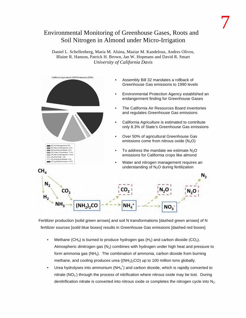
Environmental Monitoring of Greenhouse Gases, Roots and Soil Nitrogen in Almond under Micro-Irrigation

Daniel L. Schellenberg, Maria M. Alsina, Maziar M. Kandelous, Andres Olivos,

Blaine R. Hanson, Patrick H. Brown, Jan W. Hopmans and David R. Smart University of California Davis

• Methane (CH4) is burned to produce hydrogen gas (H2) and carbon dioxide (CO2).

Atmospheric dinitrogen gas (N2) combines with hydrogen under high heat and pressure to

form ammonia gas (NH3). The combination of ammonia, carbon dioxide from burning

methane, and cooling produces urea ((NH2)2CO) up to 100 million tons globally.

• Urea hydrolyses into ammonium (NH4+) and carbon dioxide, which is rapidly converted to

nitrate (NO3-) through the process of nitrification where nitrous oxide may be lost. During

denitrification nitrate is converted into nitrous oxide or completes the nitrogen cycle into N2.

• Assembly Bill 32 mandates a rollback of Greenhouse Gas emissions to 1990 levels

• Environmental Protection Agency established an

endangerment finding for Greenhouse Gases • The California Air Resources Board inventories

and regulates Greenhouse Gas emissions • California Agriculture is estimated to contribute

only 8.3% of State’s Greenhouse Gas emissions • Over 50% of agricultural Greenhouse Gas

emissions come from nitrous oxide (N2O) • To address the mandate we estimate N2O

emissions for California crops like almond

• Water and nitrogen management requires an understanding of N2O during fertilization

Fertilizer production [solid green arrows] and soil N transformations [dashed green arrows] of N

fertilizer sources [soild blue boxes] results in Greenhouse Gas emissions [dashed red boxes]

7

• Roots collected during a initial survey in July 2010 give background information

• Minirhizotron imagery provides insight into root production rates

• Root monitoring offers the opportunity to observe roots in situ

Modeling Soil Water and Nitrogen using HYDRUS-2D

Given the collection of valuable data sets by UC researchers, modeling provides the next step to generate

predictions for a host of management scenarios and almond-growing locations throughout California.

Objectives of the HYRUS model:

• To evaluate the results of the HYDRUS-2D model using extensive field data

• To determine optimal irrigation and fertigation practices for micro-irrigation

• To improve water and nitrate use efficiencies

• To reduce leaching and gaseous losses of nitrogen

The soil profile, hydraulic properties and evapotranspiration from weather station along with

irrigation/fertigation rate for each irrigation system will be used as an input file for the numerical model

HYDRUS-2D to simulate soil water movement, solute transport and root water uptake.

Top view of the soil sensor installation Sensors at different depth in the root zone

Root monitoring using minirhizotron images – pictures taken on May 3rd (left) and May 16th (right)

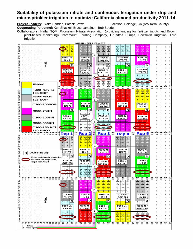
Suitability of potassium nitrate and continuous fertigation under drip and microsprinkler irrigation to optimize California almond productivity 2011-14 Project Leaders: Blake Sanden, Patrick Brown Location: Belridge, CA (NW Kern County) Cooperating Personnel: Ken Shackel, Bruce Lampinen, Bob Beede Collaborators: Haifa, SQM, Potassium Nitrate Association (providing funding for fertilizer inputs and Brown

plant-based monitoring), Paramount Farming Company, Grundfos Pumps, Bowsmith Irrigation, Toro Irrigation

30 - - - - - - - + + + + + + + + + + + + + + + - - - -29 - - - - - - - 24 25 72 73 120 121 168 169 216 217 264 265 312 313 360 - - - -28 - - - - - - - + + + + + + + + + + + + + + + - - - -27 - - - - - - - 23 26 71 74 119 122 167 170 215 218 263 266 311 314 359 - - - -26 - - - - - - - + + + + + + + + + + + + + + + - - - -25 - - - - - - - 22 27 70 75 118 123 166 171 214 219 262 267 310 315 358 - - - -24 - - - - - - - + + + + + + + + + + + + + + + - - - -23 - - - - - - - + + + + + + + + + + + + + + + - - - -22 - - - - - - - + + + + + + + + + + + + + + + - - - -21 - - - - - - - + + + + + + + + + + + + + + + - - - -20 - - - - - - - + + + + + + + + + + + + + + + - - - -19 - - - - - - - + + + + + + + + + + + + + + + - - - -18 - - - - - - - + + + + + + + + + + + + + + + - - - -17 - - - - - - - + + + + + + + + + + + + + + + - - - -16 - - - - - - - + + + + + + + + + + + + + + + - - - -15 - - - - - - - + + + + + + + + + + + + + + + - - - -14 - - - - - - - + + + + + + + + + + + + + + + - - - -13 - - - - - - - + + + + + + + + + + + + + + + - - - -12 - - - - - - - + + + + + + + + + + + + + + + - - - -11 - - - - - - - + + + + + + + + + + + + + + + - - - -10 - - - - - - - + + + + + + + + + + + + + + + - - - -9 - - - - - - - + + + + + + + + + + + + + + + - - - -8 - - - - - - - + + + + + + + + + + + + + + + - - - -7 - - - - - - - + + + + + + + + + + + + + + + - - - -6 - - - - - - - 21 28 69 76 117 124 165 172 213 220 261 268 309 316 357 - - - -5 - - - - - - - + + + + + + + + + + + + + + + - - - -4 - - - - - - - 20 29 68 77 116 125 164 173 212 221 260 269 308 317 356 - - - -3 - - - - - - - + + + + + + + + + + + + + + + - - - -2 - - - - - - - 19 30 67 78 115 126 163 174 211 222 259 270 307 318 355 - - - -1 - - - - - - - + + + + + + + + + + + + + + + - - - -

M NP M NP M NP M NP M NP M NP M NP M NP M NP M NP M NP M NP M NP M NP M NP M NP M NP M NP M1 2 3 4 5 6 7 8 9 10 11 12 13 14 15 16 17 18 19 20 21 22 23 24 25 26 27 28 29 30 31 32 33 34 35 36 37

31 - - - - - - - + + + + + + + + + + + + + + + - - - -30 - - - - - - - 18 31 66 79 114 127 162 175 210 223 258 271 306 319 354 - - - -29 - - - - - - - + + + + + + + + + + + + + + + - - - -28 - - - - - - - 17 32 65 80 113 128 161 176 209 224 257 272 305 320 353 - - - -27 - - - - - - - + + + + + + + + + + + + + + + - - - -26 - - - - - - - 16 33 64 81 112 129 160 177 208 225 256 273 304 321 352 - - - -25 - - - - - - - + + + + + + + + + + + + + + + - - - -24 - - - - - - - + + + + + + + + + + + + + + + - - - -23 - - - - - - - + + + + + + + + + + + + + + + - - - -22 - - - - - - - + + + + + + + + + + + + + + + - - - -21 - - - - - - - + + + + + + + + + + + + + + + - - - -20 - - - - - - - + + + + + + + + + + + + + + + - - - -19 - - - - - - - + + + + + + + + + + + + + + + - - - -18 - - - - - - - + + + + + + + + + + + + + + + - - - -17 - - - - - - - + + + + + + + + + + + + + + + - - - -16 - - - - - - - + + + + + + + + + + + + + + + - - - -15 - - - - - - - + + + + + + + + + + + + + + + - - - -14 - - - - - - - + + + + + + + + + + + + + + + - - - -13 - - - - - - - + + + + + + + + + + + + + + + - - - -12 - - - - - - - + + + + + + + + + + + + + + + - - - -11 - - - - - - - + + + + + + + + + + + + + + + - - - -10 - - - - - - - + + + + + + + + + + + + + + + - - - -9 - - - - - - - + + + + + + + + + + + + + + + - - - -8 - - - - - - - + + + + + + + + + + + + + + + - - - -7 - - - - - - - + + + + + + + + + + + + + + + - - - -6 - - - - - - - 15 34 63 82 111 130 159 178 207 226 255 274 303 322 351 - - - -5 - - - - - - - + + + + + + + + + + + + + + + - - - -4 - - - - - - - 14 35 62 83 110 131 158 179 206 227 254 275 302 323 350 - - - -3 - - - - - - - + + + + + + + + + + + + + + + - - - -2 - - - - - - - 13 36 61 84 109 132 157 180 205 228 253 276 301 324 349 - - - -1 - - - - - - - + + + + + + + + + + + + + + + - - - -


30 - - - - - - - + + + + + + + + + + + + + + + - - - -29 - - - - - - - 12 37 60 85 108 133 156 181 204 229 252 277 300 325 348 - - - -28 - - - - - - - + + + + + + + + + + + + + + + - - - -27 - - - - - - - 11 38 59 86 107 134 155 182 203 230 251 278 299 326 347 - - - -26 - - - - - - - + + + + + + + + + + + + + + + - - - -25 - - - - - - - 10 39 58 87 106 135 154 183 202 231 250 279 298 327 346 - - - -24 - - - - - - - + + + + + + + + + + + + + + + - - - -23 - - - - - - - + + + + + + + + + + + + + + + - - - -22 - - - - - - - + + + + + + + + + + + + + + + - - - -21 - - - - - - - + + + + + + + + + + + + + + + - - - -20 - - - - - - - + + + + + + + + + + + + + + + - - - -19 - - - - - - - + + + + + + + + + + + + + + + - - - -18 - - - - - - - + + + + + + + + + + + + + + + - - - -17 - - - - - - - + + + + + + + + + + + + + + + - - - -16 - - - - - - - + + + + + + + + + + + + + + + - - - -15 - - - - - - - + + + + + + + + + + + + + + + - - - -14 - - - - - - - + + + + + + + + + + + + + + + - - - -13 - - - - - - - + + + + + + + + + + + + + + + - - - -12 - - - - - - - + + + + + + + + + + + + + + + - - - -11 - - - - - - - + + + + + + + + + + + + + + + - - - -10 - - - - - - - + + + + + + + + + + + + + + + - - - -9 - - - - - - - + + + + + + + + + + + + + + + - - - -8 - - - - - - - + + + + + + + + + + + + + + + - - - -7 - - - - - - - + + + + + + + + + + + + + + + - - - -6 - - - - - - - 9 40 57 88 105 136 153 184 201 232 249 280 297 328 345 - - - -5 - - - - - - - + + + + + + + + + + + + + + + - - - -4 - - - - - - - 8 41 56 89 104 137 152 185 200 233 248 281 296 329 344 - - - -3 - - - - - - - + + + + + + + + + + + + + + + - - - -2 - - - - - - - 7 42 55 90 103 138 151 186 199 234 247 282 295 330 343 - - - -1 - - - - - - - + + + + + + + + + + + + + + + - - - -


30 - - - - - - - + + + + + + + + + + + + + + + - - - -29 - - - - - - - 6 43 54 91 102 139 150 187 198 235 246 283 294 331 342 - - - -28 - - - - - - - + + + + + + + + + + + + + + + - - - -27 - - - - - - - 5 44 53 92 101 140 149 188 197 236 245 284 293 332 341 - - - -26 - - - - - - - + + + + + + + + + + + + + + + - - - -25 - - - - - - - 4 45 52 93 100 141 148 189 196 237 244 285 292 333 340 - - - -24 - - - - - - - + + + + + + + + + + + + + + + - - - -23 - - - - - - - + + + + + + + + + + + + + + + - - - -22 - - - - - - - + + + + + + + + + + + + + + + - - - -21 - - - - - - - + + + + + + + + + + + + + + + - - - -20 - - - - - - - + + + + + + + + + + + + + + + - - - -19 - - - - - - - + + + + + + + + + + + + + + + - - - -18 - - - - - - - + + + + + + + + + + + + + + + - - - -17 - - - - - - - + + + + + + + + + + + + + + + - - - -16 - - - - - - - + + + + + + + + + + + + + + + - - - -15 - - - - - - - + + + + + + + + + + + + + + + - - - -14 - - - - - - - + + + + + + + + + + + + + + + - - - -13 - - - - - - - + + + + + + + + + + + + + + + - - - -12 - - - - - - - + + + + + + + + + + + + + + + - - - -11 - - - - - - - + + + + + + + + + + + + + + + - - - -10 - - - - - - - + + + + + + + + + + + + + + + - - - -9 - - - - - - - + + + + + + + + + + + + + + + - - - -8 - - - - - - - + + + + + + + + + + + + + + + - - - -7 - - - - - - - + + + + + + + + + + + + + + + - - - -6 - - - - - - - 3 46 51 94 99 142 147 190 195 238 243 286 291 334 339 - - - -5 - - - - - - - + + + + + + + + + + + + + + + - - - -4 - - - - - - - 2 47 50 95 98 143 146 191 194 239 242 287 290 335 338 - - - -3 - - - - - - - + + + + + + + + + + + + + + + - - - -2 - - - - - - - 1 48 49 96 97 144 145 192 193 240 241 288 289 336 337 - - - -1 - - - - - - - + + + + + + + + + + + + + + + - - - -


NORTH -- SET 1 FANJETSFl

atFl

at

Rep 4

Flat

Flat

Flat

4

5

C300 NKN 300

C300 NKN 200

FiltersFertilzer Inject

D

D

7

8

F300 UNKTS 75

F300 UNKTS 75

F300 UNKTS 75

D

F300 NKN 75

D

F300 UNKTS 75

F300 UNKTS 75

DC300 N

SOP 200

C300 NSOP 200

C300 NSOP

C300 NKN 75

D

C300 NSOP 200

D

C300 NKN 300

D

D

F300 UNK = 0

F300 UNK = 0

F300 UNK = 0

F300 UNK = 0

F300 UNK = 0

F300 NKN 75

D

F300 NKN 75

D

F300 NKN 75

D

C300 NKN 75

D

C300 NKN 75

D

C300 NKN 75

D

D

C300 NKN 200

D

C300 NKN 200

D

C300 NKN 200

D

D

6

3

1

2

Rep 1 Rep 2 Rep 3 Rep 5

C300 NKN 200

C300 NSOP 200

D

C300 NKN 300

C300 NKN 75

C300 NKCl 150

C300 NKN 300

F300 NKN 75

C300 NKN 300

Double-line drip

Weekly neutron probe monitor-ing, annual soil sampling to 9 feet, Nonprl, Mont, Nonprl

D

C300-150 KCl 150 KNO3

C300-200SOP

C300-75KN

C300-200KN

C300-300KN

F300-75KN125 SOP

F300-0

F300-75KTS125 SOP

C300 NKCl 150

C300 NKCl 150

C300 NKCl 150

C300 NKCl 150

KNO3 CONTINUOUS FERTIGATION TRIAL

Double-line drip

G: 300 lb K as KNO3 and 128 lbs N as UAN (total N 300) continuous. (Manifold 4)

H: 150 lb K as KCL, 150 lb K as KNO3, 248 lbs N as UAN continuous fertigation. (Manifold 5)C300-150 KCl 150 KNO3

C300-200SOP

C300-75KN

C300-200KN

C300-300KN

C: 200 lb K. 125 lb K as SOP band February, 75 lb as KNO3 and 273 lb N as UAN in 4 in season fertigations 20% Feb, 30% April, 30% June, 20% post harvest.

F300-75KN125 SOP

F300-0 A: No K, 300 lbs N as UAN in 4 in season fertigations 20% Feb, 30% April, 30% June, 20% post harvest.

F300-75KTS125 SOP

B: 200 lb K. 125 lb K as SOP band February, 75 lb as KTS and 300 lb N as UAN in 4 in season fertigations 20% Feb, 30% April, 30% June, 20% post harvest (Grower Standard).

D: 200 lb K as SOP dissolved in gypsum mixer and 300 lbs N as UAN (total N 300), continuous application. (Manifold 1)E: 200 lb K. 125 lb K as SOP in band February, plus 75 lb K as KNO3 and 273 lb UAN continuous. (Manifold 2)

F: 200 lb K as KNO3 and 193 lbs N as UAN (total N 300) as continuous application. (Manifold 3)

Weekly neutron probe monitoring, annual soil sampling to 9 feet, Nonprl, Mont, NonprlD

TREATMENTS KNO3 CONTINUOUS FERTIGATION TRIAL LAYOUT

There are 5 mainlines in the drawing: one for each of the continuous fertigation treatments (5 total). Thus, all mixing and fertilizer injection occurs at the pump/filter station and flows in its own mainline to each manifold run, 1 through 5, where the solution enters the one manifold line for each respective treatment as indicated. All treatments have DRIP and FANJET irrigation on Nonpareil to test for system differences.

The 4 times/year fertigation treatments will be done with the standard plumbing for the block. Treatment (B) is essentially the Control/standard for this block. The rows designated for treatments (A) (no K) and C (75 lbs K as fertigated KNO3) will simply be turned off during the 1 to 2 hour injection of KTS 4 times/year. The KNO3 for Treatment (C) will be injected at the hoses with a mobile tank/injection unit and hose valves turned off before the end of the UN32 injection to maintain total N @ 300 lb/ac. Ground applied SOP using a Ranchero will be laid down in dual 8 inch bands at the edge of the berm in January @ 125 lb K/ac for treatments (B), (C) and (E). =============================================================================================== SUMMER MICRO IRRIGATION SYSTEMS TUNE-UP: Why use drip or microsprinklers?

The first answer most people gave 10 to 15 years ago was, “Save water.” For most growers in Kern County, this is about the last reason they’d give. Potential water savings alone do not pay for a micro system. The following list is my favorite ranking of reasons to consider micro systems.

1) Minimize stress: This actually increases ET which increases photosynthesis and carbohydrate production. Benefits can be reduced mite infestations and better fruit set in almonds.

2) Irrigation scheduling/uniformity: Applied water is a mechanical function of system capacity and not the uncertain infiltration rate of flood water into the ground. More uniform application. Knowing this amount makes it easier to …

3) Manage stress: Better control of deficit irrigation to harden trees before shaking, improve splits in pistachios or to improve characteristics of varietal wines. Encourage fruit set in tomatoes and peppers.

4) Fine-tune fertilization: Apply when plant needs it. No field compaction from shanking. Costs only for material. Fertilizer leaching is decreased or eliminated. Phosphoric acid is concentrated in small wetted areas with drip. Soluble gypsum can be injected anytime.

5) Disease management: Drip only. Decrease humidity. 6) Save WASTED water!

How uniform is the average micro system in Kern?

Over 400 field evaluations, the Irrigation Mobile Lab in Kern County, CA found that average DU for drip systems was only slightly better than furrow irrigation (75 compared to 72%). Micro-sprinkler systems averaged 78%. This was not due to poor design, but lack of maintenance. Some of these systems were later tuned up to 85%. A system with 75% DU takes 16% more water to adequately irrigate than a 90% system.

How can I tune-up my micro system? 1) Check in-field emitter type. The single most important thing to check is that you have the same type of emitters throughout the field. The biggest reason that average micro irrigation DU drops is because clogged emitters or micro-sprinkler heads are replaced with others that have a different flow rate than the old system. Not only is the same flow rate critical, but it is a good idea to stick with the same brand so that the flow curve for different pressures will be the same. If your satisfied that you have uniform emitters in the field then go back to the filter station. 2) Clean the filter station. Growers generally do a good job at keeping screen and disk filters clean and functioning because these clog up too quickly to be ignored. Sand media filters may need some help in the spring. Open the porthole in the tank and scoop out some sand from against the side of the tank. If it falls apart and is not slimy and the level of sand is about two thirds full then you’re set. If the sand is chunky then you have some algae growth that will decrease the effectiveness of the filter and cause excessive back flushing. Close the valve to the field. Leave the portholes open. Turn on the pump to just fill the tanks and then shut down. Dump in about a half gallon of bleach for a 4 foot diameter tank and leave it sit overnight. Close up the portholes and open the field valve a quarter of the way and set the back flush cycle for 90 seconds. Turn the booster on and adjust the backpressure to give about 50 to 60 psi. Put a bucket under the back flush outlet to make sure your not blowing sand out. When all filters have back flushed keep the booster running and open the field valve to adjust for design field pressure. 3) Check subunit regulator pressures and operation. Next to mixed emitters this is the biggest problem in large systems. For large acreage sets there may be 20 or more pressure regulators in the field. These can be as simple as a gate valve or as complex as a $200 diaphragm operated self-adjusting pressure regulator with a solenoid for automatic cycling. Achieving uniform pressure to all your irrigation laterals is easier with self-adjusting regulators when they function correctly. Using two pressure gauges check the upstream and downstream pressure at the regulator. Set the downstream pressure to system design. You should have 5 to 15 psi more pressure going into the regulator than coming out. Slowly close the gate valve in front of the regulator so you go from say 12 psi difference to a 6 to 8 psi difference across the regulator. The downstream pressure should stay the same. If this pressure drops then you need to clean or rebuild the regulator. Sometimes this means only cleaning accumulated silt out of the pilot valve, or it may mean replacing springs and/or diaphragms. Consult the manufacturer. Adjust subunit pressures starting closest to the pump. Go through the field twice. 4) Check hose screens. These little troublemakers can be as bad as the above problem, and can be worse from the standpoint of plugging up multiple times during the season. These are little 60 to 80 mesh screens molded in the gasket that makes the seal between the riser and the hose. Made as a safeguard to prevent sand from plugging a hose and emitters if there was a blowout, these things can collect filamentous algae and cause pressure drops of 15 psi. If you use canal water you will get algal spores and filaments in the water that can snake through the sand media and get trapped on these little screens. Dedicate your self to cleaning these every 2 to 3 weeks or throw them out and use plain washers. Over the last 11 years I have never seen these screens ‘save’ a system, but I have seen many settings where one hose only has 8 psi and the one next to it has 22 psi. 5) Flush hoses and check for algae, slime, etc. Open only 10 to 15 hoses at a time to get good velocity. Put a nylon sock over the end and check for the type of material flushed out. If the water clears in 10 to 15 seconds and the solids are mostly suspended clays, then you’re probably okay. Any slime or algae means that you need to sanitize the system within the month. Injection of chlorine, as a gas or bleach, is the most common material. 6) Check individual, random emitters for flow rate. Once pressures are properly adjusted and all hoses in the set are clean, put out little catch cans for drippers or use milk jugs for microsprinklers, and measure the flow. Compare this to the pressure/flow curve of the emitter when it was new. Check a total of 40 emitters from different areas. If the average flow is more than 10% different from the design specifications than you should consider new emitters. Divide the average flow from the lowest 10 emitters by the overall average to get the DU of your system.

Documents

Almond Irrigation, Nutrition for High Yield and