V

Alneelain University

Faculty of Graduate Studies

Performance Evaluation of LTE Handover using TTTAlgorithm

A Thesis Submitted in Fulfillment for the Degree of M.Sc. in Network

By:

WALAA FAISAL MOHAMMED ABDALLH

Supervisor :Dr. Ahmed M. Alhassan .

December 2018

II

الآية

قال تعالى:

يله إ�لا و�� { وما يع�لم تأ

خون ف�ي اس� الله و الر

ال�ع�ل�م� يقولون آمنا ب�ه�

1

ن�د� كل م�ن� ع�

ل�باربنا أولوالأ� ومايذكرإ�لا

{ب�

]7] آل عمران :

2

Acknowledgement

Firstly, I would like to express my sincere gratitude to my advisor DR.

AHMED HASSAN MOHAMMED HASSAN for the continuous

support of my M.Sc. study, for his patience, motivation, and immense

knowledge. His guidance helped me in all the time of research and

writing of this thesis. I could not have imagined having a better advisor

and mentor for my M.Sc. study.

My sincere thanks also go to Dr. Ahmed M. Alhassan for his insightful

comments and encouragement, but also for the hard question which

incented me to widen my research from various perspectives.

Last but not the least; I would like to thank my family for supporting me

spiritually throughout writing this thesis and in my life in general.

3

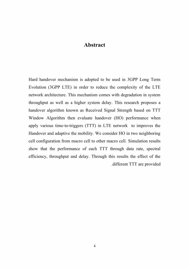
Abstract

Hard handover mechanism is adopted to be used in 3GPP Long Term

Evolution (3GPP LTE) in order to reduce the complexity of the LTE

network architecture. This mechanism comes with degradation in system

throughput as well as a higher system delay. This research proposes a

handover algorithm known as Received Signal Strength based on TTT

Window Algorithm then evaluate handover (HO) performance when

apply various time-to-triggers (TTT) in LTE network to improves the

Handover and adaptive the mobility. We consider HO in two neighboring

cell configuration from macro cell to other macro cell. Simulation results

show that the performance of each TTT through data rate, spectral

efficiency, throughput and delay. Through this results the effect of the

different TTT are provided .

4

المستخلص

آلية عملية التسليم تم استخدامها في الجيل الرابع لتسهيل التعقيد في معمارية الش99بكة .

هذه الالي9ة ت9ودي الى نقص9ان الانتاجي9ة و زي9ادة الت9أخير مم9ا ي9ودي الى ت9دني ج9ودة

الشبكة .

ه9ذا البحث يق9دم خوارزمي9ة ق9وة الاش9ارة المس9تقبلة بالاعتم9اد على ال9زمن لتحس9ين

عملية التس9ليم ثم تط9بيق اداء عملي9ة التس9ليم عن9د قيم مختلف9ة لل9زمن في ش9بكة الجي9ل

الرابع .

فرضنا أن عملية التسليم تمت من خلية صغيرة الى خلية صغيرة أخرى وتطبيق هذه

العملية باستخدام برنامج الماتلاب و استخراج نتائج اداء عملية التس99ليم لك99ل زمن و

معدل نق9ل البيان9ات , كف9اءة الش9بكة , و الت9اخير في الانتق9ال وتأثير هذه العملية على

على جودة الش9بكة بش9كل ع9ام . خلال ه9ذه النت9ائج تم التحق9ق من ت9أثير ال9زمن على

عملية التسليم بأخذ قيم مختلفة لزمن .

5

Table of Contents

1 CHAPTER ONE – INTRODUCTION..........................................................................1

1.1 General View............................................................................................................1

1.2 Problem Statement....................................................................................................2

1.3 Objective...................................................................................................................2

1.4 Methodology.............................................................................................................2

1.5 Thesis Overview.......................................................................................................2

2 CHAPTER TWO – THEORETICAL BACKGROUND AND RELATED WORK..3

2.1 Overview of cellular generations..............................................................................3

2.1.1 First Generation (1G)........................................................................................3

2.1.2 Second generation (2G).....................................................................................4

2.1.3 Third Generation (3G).......................................................................................6

2.1.4 Fourth Generation (4G)...................................................................................10

2.2 Long Term Evolution (LTE):..................................................................................12

2.3 Heterogeneous Networks........................................................................................14

2.4 Related work...........................................................................................................15

6

3 CHAPTER THREE – LTE Handover........................................................................19

3.1 Introduction.............................................................................................................19

3.2 HANDOVER MECHANISMS...............................................................................19

3.3 Handover theory:....................................................................................................20

3.4 Requirements for an efficient handover..................................................................21

3.4.1 Handover moment...........................................................................................21

3.4.2 Unnecessary handovers...................................................................................21

3.4.3 Handover delay...............................................................................................21

3.4.4 Packet loss.......................................................................................................21

3.4.5 Scalability.......................................................................................................22

3.4.6 Complexity......................................................................................................22

3.5 Handover techniques...............................................................................................22

3.5.1 Soft handover, Connect-Before-Break............................................................22

3.5.2 Hard handover, Break-Before-Connect...........................................................22

3.6 Handover in LTE....................................................................................................23

3.6.1 Types of Handover in LTE network................................................................23

3.7 LTE Hard Handover Algorithm..............................................................................26

3.8 Received Signal Strength based on TTT Window Algorithm.................................28

3.9 Mathematical Model...............................................................................................29

3.9.1 Signal to interference noise ratio (SINR)........................................................29

3.9.2 Data rate (DR).................................................................................................30

7

3.9.3 Throughput (TH).............................................................................................30

3.9.4 Spectral Efficiency (SE)..................................................................................30

3.9.5 Delay transmission (DT).................................................................................31

3.10 Simulation Model:..................................................................................................32

3.11 System Model Flow Chart......................................................................................33

4 CHAPPTER FOUR- SIMULATION AND RESULT................................................34

4.1 Simulation Results..................................................................................................34

4.1.1 Signal to interference noise ratio (SINR)........................................................35

4.1.2 Data rate..........................................................................................................35

4.1.3 Accumulated Throughput................................................................................36

4.1.4 Spectral Efficiency..........................................................................................37

4.1.5 Delay Transition..............................................................................................37

5 CHAPPTER FIVE – CONCLUSSION AND RECOMMENDATIONS...................38

5.1 Conclusion..............................................................................................................38

5.2 RECOMMENDATIONS........................................................................................38

Reference:..............................................................................................................................39

6 Appendix.......................................................................................................................40

8

List of Figures

Figure 2-1UMTS Architecture................................................................................................10

Figure 2-2 LTE architecture....................................................................................................13

Figure 2-3 Heterogeneous Networks......................................................................................15

Figure 2-4 handover algorithm...............................................................................................17

Figure 3-1 Handover region....................................................................................................19

Figure 3-2 Handover a) handover-successful b) handover-un successful...............................20

Figure 3-3 LTE handover.......................................................................................................24

Figure 3-4 LTE Hard Handover Algorithm...........................................................................27

Figure 4-1 SINR Macro1 and Macro2 with two Handover scenario.......................................34

Figure 4-2 Data Rate of HO1&HO2.......................................................................................35

Figure 4-3 Accumulated Throughput......................................................................................35

Figure 4-4 Spectral Efficiency................................................................................................36

Figure 4-5 Delay Transition....................................................................................................36

9

List of Tables

Table 2.2: Related work

summary………………………………………………………18

Table 4.1: Simulation

Parameters………………………………………………………..33

10

1List of Symbols

Symbol

BW

C

D

DR

DT

G

I

M

N

PR

Description

Bandwidth

Coding Rate

Data

Data Rate

Delay Transmission

Gain of antenna

Interference

Modulation level

Noise

Power Receive in Mobile SINR Signal to interference and noise ratio

TH Throughput

11

2List of Abbreviations

Abbreviation Description

1G First Generation

2G Second Generation

3G Third Generation

3GPP Third Generation Partnership Project

3GPP2 Third Generation Partnership Project2

64 QAM

AMC

AMPS

C

CDMA

CR

DL

D-eNB

EDGE

64 Quarter Phase Shift Keying

Adaptive Modulation and Coding

Advance Mobile Phone System

Capacity

Code Division Multiple Access

Code Rat e

Down Link

Destination eNB

Enhanced Data rate for Global Evolution

12

eNode Evolved NodeB

E-UTRAN Evolved UMTS Terrestrial Radio Access Network

FDD Frequency Division Duplex

Gbps Gigabit Per Second

GSM Global System For Mobile Communication

GPRS General Packet Radio Services

GW Gateway

HET NET

HOM

HSS

HSPA

IP

Heterogeneous Network

Handover Margin

Home Subscriber Server

High Speed Packet Access

Internet Protocol

ITU International Telecommunication union

ITU-IMT-2000 International Telecommunication union –International Mobile

Telecommuncation-2000

LTE Long Tern Evaluation

LTE –A Long Tern Evaluation-Advanced

13

MIMO Multiple Input Multiple Output

MME Mobility Management Entity

OFDM Orthogonal Frequency Multiple

OFDMA

PCRF

Orthogonal Frequency Multiple Access

Policy Control and Charging Rules Function

QAM Quarter Amplitude Modulation

RAN

RF

Radio Access Network

Radio Frequency

RNC Radio Network Controller

RSRP

S-eNB

Reference Signal Received Power

Source eNB

TTT Time to Trigger

14

Table of Contents

1 CHAPTER ONE – INTRODUCTION..........................................................................1

1.1 General View............................................................................................................1

1.2 Problem Statement....................................................................................................2

1.3 Objective...................................................................................................................2

15

1.4 Methodology.............................................................................................................2

1.5 Thesis Overview.......................................................................................................2

2 CHAPTER TWO – THEORETICAL BACKGROUND AND RELATED WORK..3

2.1 Overview of cellular generations..............................................................................3

2.1.1 First Generation (1G)........................................................................................3

2.1.2 Second generation (2G).....................................................................................4

2.1.3 Third Generation (3G).......................................................................................6

2.1.4 Fourth Generation (4G)...................................................................................10

2.2 Long Term Evolution (LTE):..................................................................................12

2.3 Heterogeneous Networks........................................................................................14

2.4 Related work...........................................................................................................15

3 CHAPTER THREE – LTE Handover........................................................................19

3.1 Introduction.............................................................................................................19

3.2 HANDOVER MECHANISMS...............................................................................19

3.3 Handover theory:....................................................................................................20

3.4 Requirements for an efficient handover..................................................................21

3.4.1 Handover moment...........................................................................................21

3.4.2 Unnecessary handovers...................................................................................21

3.4.3 Handover delay...............................................................................................21

3.4.4 Packet loss.......................................................................................................21

3.4.5 Scalability.......................................................................................................22

16

3.4.6 Complexity......................................................................................................22

3.5 Handover techniques...............................................................................................22

3.5.1 Soft handover, Connect-Before-Break............................................................22

3.5.2 Hard handover, Break-Before-Connect...........................................................23

3.6 Handover in LTE....................................................................................................23

3.6.1 Types of Handover in LTE network................................................................23

3.7 LTE Hard Handover Algorithm..............................................................................26

3.8 Received Signal Strength based on TTT Window Algorithm.................................28

3.9 Mathematical Model...............................................................................................29

3.9.1 Signal to interference noise ratio (SINR)........................................................29

3.9.2 Data rate (DR).................................................................................................30

3.9.3 Throughput (TH).............................................................................................30

3.9.4 Spectral Efficiency (SE)..................................................................................31

3.9.5 Delay transmission (DT).................................................................................31

3.10 Simulation Model:..................................................................................................32

3.11 System Model Flow Chart......................................................................................33

4 CHAPPTER FOUR- SIMULATION AND RESULT................................................34

4.1 Simulation Results..................................................................................................34

4.1.1 Signal to interference noise ratio (SINR)........................................................35

4.1.2 Data rate..........................................................................................................35

4.1.3 Accumulated Throughput................................................................................36

17

4.1.4 Spectral Efficiency..........................................................................................37

4.1.5 Delay Transition..............................................................................................37

5 CHAPPTER FIVE – CONCLUSSION AND RECOMMENDATIONS...................38

5.1 Conclusion..............................................................................................................38

5.2 RECOMMENDATIONS........................................................................................38

Reference:..............................................................................................................................39

6 Appendix.......................................................................................................................40

List of Figures

Figure 2-1UMTS Architecture................................................................................................10

Figure 2-2 LTE architecture....................................................................................................13

Figure 2-3 Heterogeneous Networks......................................................................................15

Figure 2-4 handover algorithm...............................................................................................17

18

Figure 3-1 Handover region....................................................................................................19

Figure 3-2 Handover a) handover-successful b) handover-un successful...............................20

Figure 3-3 LTE handover.......................................................................................................25

Figure 3-4 LTE Hard Handover Algorithm......................................................................27

Figure 4-1 SINR Macro1 and Macro2 with two Handover scenario................................35

Figure 4-2 Data Rate of HO1&HO2.......................................................................................36

Figure 4-3 Accumulated Throughput......................................................................................36

Figure 4-4 Spectral Efficiency................................................................................................37

Figure 4-5 Delay Transition....................................................................................................37

19

1 CHAPTER ONE – INTRODUCTION

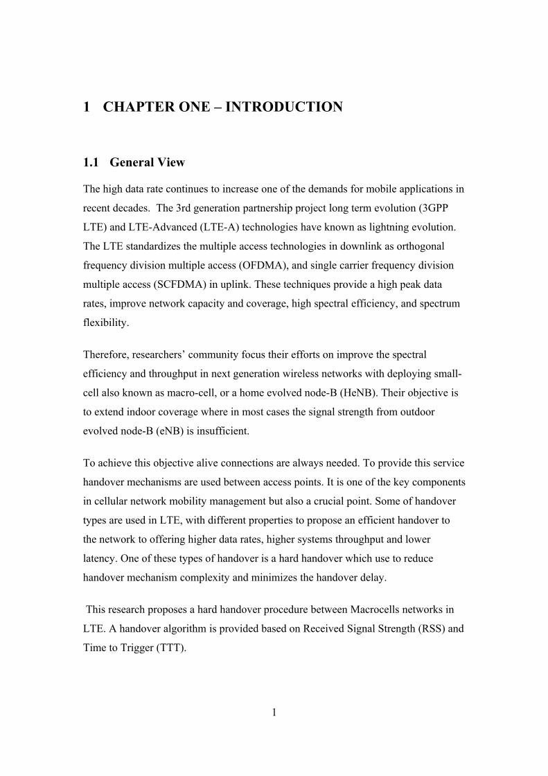
1.1 General View

The high data rate continues to increase one of the demands for mobile applications in

recent decades. The 3rd generation partnership project long term evolution (3GPP

LTE) and LTE-Advanced (LTE-A) technologies have known as lightning evolution.

The LTE standardizes the multiple access technologies in downlink as orthogonal

frequency division multiple access (OFDMA), and single carrier frequency division

multiple access (SCFDMA) in uplink. These techniques provide a high peak data

rates, improve network capacity and coverage, high spectral efficiency, and spectrum

flexibility.

Therefore, researchers’ community focus their efforts on improve the spectral

efficiency and throughput in next generation wireless networks with deploying small-

cell also known as macro-cell, or a home evolved node-B (HeNB). Their objective is

to extend indoor coverage where in most cases the signal strength from outdoor

evolved node-B (eNB) is insufficient.

To achieve this objective alive connections are always needed. To provide this service

handover mechanisms are used between access points. It is one of the key components

in cellular network mobility management but also a crucial point. Some of handover

types are used in LTE, with different properties to propose an efficient handover to

the network to offering higher data rates, higher systems throughput and lower

latency. One of these types of handover is a hard handover which use to reduce

handover mechanism complexity and minimizes the handover delay.

This research proposes a hard handover procedure between Macrocells networks in

LTE. A handover algorithm is provided based on Received Signal Strength (RSS) and

Time to Trigger (TTT).

1

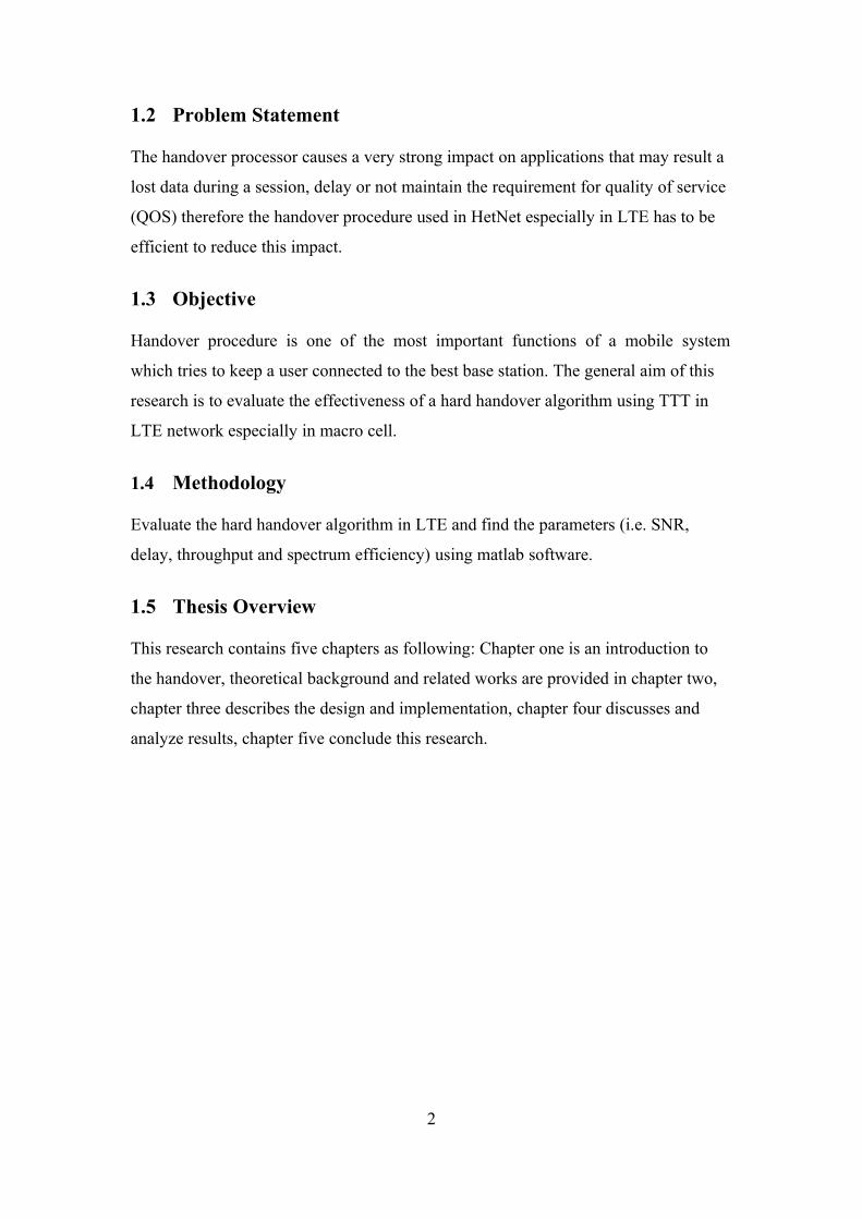
1.2 Problem Statement

The handover processor causes a very strong impact on applications that may result a

lost data during a session, delay or not maintain the requirement for quality of service

(QOS) therefore the handover procedure used in HetNet especially in LTE has to be

efficient to reduce this impact.

1.3 Objective

Handover procedure is one of the most important functions of a mobile system

which tries to keep a user connected to the best base station. The general aim of this

research is to evaluate the effectiveness of a hard handover algorithm using TTT in

LTE network especially in macro cell.

1.4 Methodology

Evaluate the hard handover algorithm in LTE and find the parameters (i.e. SNR,

delay, throughput and spectrum efficiency) using matlab software.

1.5 Thesis Overview

This research contains five chapters as following: Chapter one is an introduction to

the handover, theoretical background and related works are provided in chapter two,

chapter three describes the design and implementation, chapter four discusses and

analyze results, chapter five conclude this research.

2

2 CHAPTER TWO – THEORETICAL BACKGROUND AND RELATED WORK

2.1 Overview of cellular generations

The cellular generation in communications system is commonly known by 1G, 2G

and 3G, 4G designations, the 3G designed for high speed data transmission.1G started

in the late 1970 and early 1980s, it was analog and it used for data like an ordinary

telephone line is used with an analog modem .with an adapter, one could plug a laptop

modem into some cell phone models and transfer data while travelling. The second

generation (2G) is a digital voice cell phone systems introduced in the 1990s which

are GSM and CDMA .also known as 2G+ or 2.5G, technologies have supported email

and internet access. These include GPRS and edge for GSM and is-95 for CDMA.

And third generation 3G is provided a high speed for multimedia data which ranging

from 128 kbps to several megabits per second .defined by the ITU under the IMT2000

global framework. 3G cell phones will support all the service to the 3G with addition

of movies and TV. 4G is the fourth generation of broadband cellular network

technology, succeeding 3G. 4G system must provide capabilities defined by

International Telecommunications Union and International Mobile

Telecommunications advanced [1].

2.1.1 First Generation (1G)

The first generation mobile systems are analog cell phone standards, and introduced

in the 1980 and used until being replaced by 2G. This generation uses frequency

modulation (FM), frequency division duplexing (FDD) and frequency division

multiple access (FDMA). Using the analog technology that provides analog speech

signals to the first generation wireless systems.

The data transmission between base station and mobile user not enough and the low

data rate that why the next generation cellular systems was applied. The 1G is not

3

secure because the systems are depend on analog systems , the conversation was a full

duplex that mean both the persons can talk & listen at a time. The billing, roaming

and call setup functionality were able by the system. Since the whole technology was

based on the analog system noise introduction into the signal during communication

was a disadvantage. In the current days this generation’s system and devices are no

more used. The standards in 1G technology are categorized by following types:

1. AMPS

AMPS are the first U.S. cellular telephone system called advanced mobile phone

system. This system uses 7-cell reuse pattern with provisions for sectoring and cell

splitting to increase capacity when needed. AMPS use FM, FDD for radio

transmission and also uses FDMA multiple access. Channel bandwidth is 30 KHz.

2. ETACS

European Total Access Communication systems (ETACS) was provided in Mid-

1980’s and is virtually identical to AMPS except it is scaled to fit in 25 KHz channels

used throughout Europe. Another difference between AMPS and ETAC is how the

telephone number of each subscriber is formatted, due to the need to accommodate

different country codes throughout Europe as opposed to area codes in U.S.

2.1.2 Second generation (2G)

The second generation mobile technology is depended on first generation mobile

technology. The disadvantages of the 1G make an emerging demand of the next

generation wireless system that provides new features like high speed data

communication as well as voice transmission.

This generation introduced in the early 1990. The access techniques used in this

generation are TDMA (time division multiple access) and CDMA (code division

multiple access) along with the frequency division duplexing (FDD) technique. The

increase in spectrum efficiency in 2G is three times compared to the 1G that why the

system capacity is three times greater than 1G. The standards in 2G technologies are

categorized by following types:

4

3. GSM

It’s an abbreviation of global system for mobile; it is very widely used 2G

technologies by most of the subscribers. The GSM supports 8 times slotted users for

every 200 KHz radio channels. The popular features of GSM are short messaging

service (SMS).

The uplink frequency (from base station to mobile station) is 890-915 MHz and

downlink frequency (from mobile station to base station) is 935-960 MHz the carrier

separation for GSM is 200 KHz and bandwidth of GSM is 25MHz.

It uses time division multiple access technique along with the frequency division

duplexing.GSM provides various types of Tele services and data services. The Tele

services include emergency calling, fax, videotext, and Tele text. One of the most

popular features of GSM is subscriber identity module (SIM) which gives a unique

identity to each subscriber.

4. CDMA

It is used in North America, Korea, Japan, China, and India, and supports 64 voice

channels per carrier that are Orthogonally coded. The upload channel frequency for it

is 824-849 MHz and the download channel frequency is 869-894 MHz .The carriers

are separated by 1.25MHz frequency. In CDMA the signal is modulated by binary

phase shift keying (BPSK) modulation with quadrature spreading at the data rate of

1.2288Mchips /sec.

Although, the 2G standard mobile technologies provides efficient voice data

transmission but the internet browsing applications are at very lower speeds. . So, for

providing higher data rate transmission for internet browsing applications, the 2G

standards are modified and a new standard called 2.5G standard is developed with

backward compatibility with 2G standard. The 2.5G technologies uses wireless

application protocols (WAP) by which the web pages are viewed by the users in a

compressed form. The 2.5G technology is evolved from the standards (GSM, PDC,

IS-95and IS136) in 2G technologies.

5

In 2.5G IS-95B standard is evolved from the CDMA-one standard in 2G which uses

channel bandwidth 1.25MHz. The high speed circuit switched data (HSCSD) is

evolved from GSM standard which allows individual user to use consecutive time

slots to obtain the higher speed data access on the GSM networks. It uses 200 KHz

channel bandwidth and provides transmission rate up to 57.6 kbps. The general packet

radio service (GPRS) includes features of both GSM, IS-136 and PDC. It provides a

packet data access which is suited for non- real time internet usage, fax, e-mail, web

browsing where the downloading speed is greater than uploading speed. The

enhanced data rate for GSM evolution is more advanced GSM standard which is

designed from the common features of GSM and IS-136. It is also referred as

enhanced GPRS.

2.1.3 Third Generation (3G)

This generation describes the updating that happened in wireless mobile

telecommunications technology around the world to use new 3G technologies. This

technology introduced in 1999 to 2010. This depending on a set of standards used for

mobile devices and networks that comply with the International Mobile

Telecommunications-2000 (IMT-2000) specifications by the International

Telecommunication Union. First country using this technology is Japan. 3G wireless

systems provide backward compatibility for 2G and 2.5G

3G telecommunication networks support services that provide an information transfer

rate of at least 0.2 Mbit/s, it is designed for higher speed internet access and different

types of web browsing applications. This application can be finds in wireless voice

telephony, mobile and fixed wireless Internet access, video calls and video

conferencing which enable multiple called parties that can communicate face to face

though they are at a long distance. It also supports multimedia service. The 3G

standard is categorized in two types which are as follows:

3GPP

This is an abbreviation of 3G partnership projects for wideband CDMA standard and

it based on backward compatibility with GSM and IS-136/PDC. This standard

involves wideband code division multiple access (W-CDMA), time division

6

synchronous code division multiple access (TD-SCDMA) and enhanced data for

GSM evolution (EDGE). The W-CDMA is also known as universal mobile

telecommunication system (UMTS), it use both frequency division duplexing (FDD)

and time division duplexing (TDD). This technique is backward compatible with

GSM and forward channel bandwidth is 5 GHz. The data rate of it is up to 2 Mbps

and spectral efficiency is six times greater than GSM system. The TD-SCDMA is a

widely popular GSM compatible standard. It has 1.6 MHz bandwidth, uses TDD

duplexing technique and the channel bit rate is up to 2.227 Mbps.

GPP-2

This an abbreviation of 3G partnership project for CDMA 2000standard. It is

backward compatible to 2G CDMA technique i.e. IS-95 and 2.5G technique i.e.IS-95

B. This standard uses both FDD and TDD duplexing methods. The downlink

frequency can be implemented using either direct spreading or multi carrier and

uplink frequencies support the simultaneous combination of multicarrier and direct

spreading. The 3G –CDMA 200 data rate is up to 2 Mbps.

UMTS is part of the IMT-2000 group of 3G mobile communication system. It is also

known as Global System for Mobile communications (3GSM) because it contained

from that system and the air interface for the UMTS network is based on Wideband

Code Division Multiple Access (WCDMA) and includes the High Speed Packet

Access (HSPA) specification. This architecture is as according to the third generation

project (3GP) requirements. Besides providing changes in the network infrastructure

the UMTS specifications Point out the evolution path from GSM circuit switched

networks towards packet switched technologies offering higher transmission rates [1].

This architecture is according to the third generation project (3GP) requirements. This

network consists of the User Equipment domain (UE), the UMTS Terrestrial Radio

Access Network (UTRAN) and the Core network part.

a) User Equipment domain

7

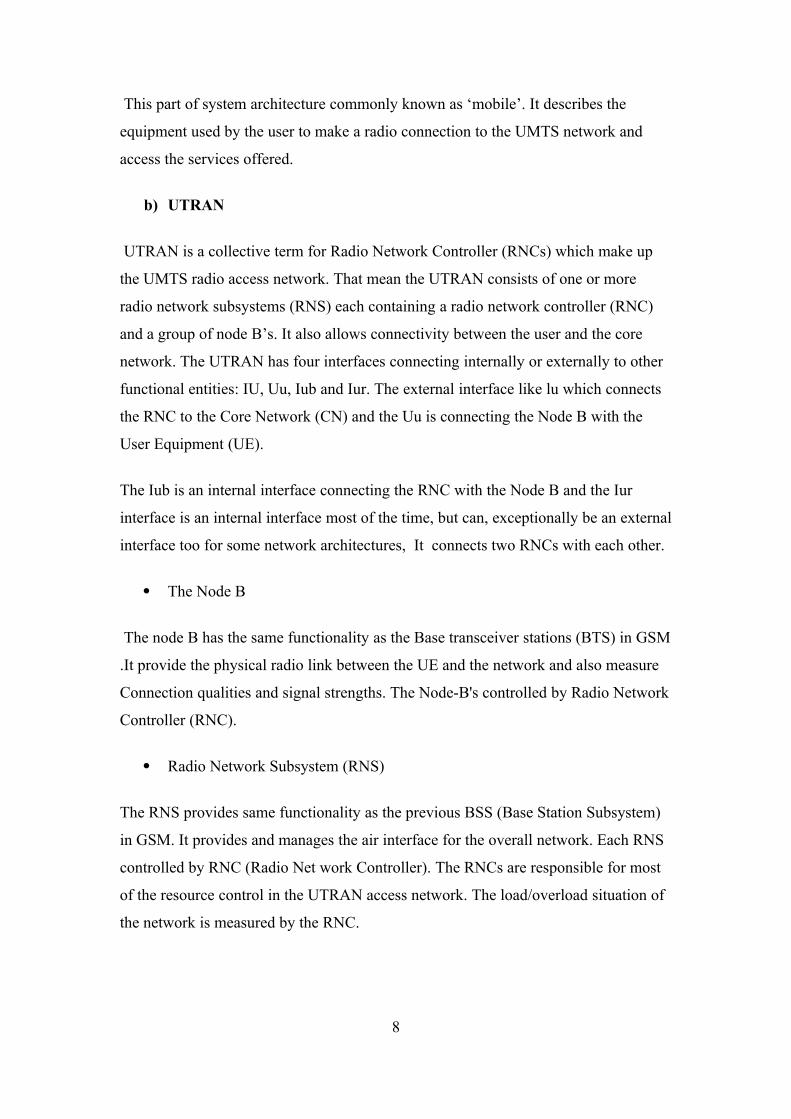
This part of system architecture commonly known as ‘mobile’. It describes the

equipment used by the user to make a radio connection to the UMTS network and

access the services offered.

b) UTRAN

UTRAN is a collective term for Radio Network Controller (RNCs) which make up

the UMTS radio access network. That mean the UTRAN consists of one or more

radio network subsystems (RNS) each containing a radio network controller (RNC)

and a group of node B’s. It also allows connectivity between the user and the core

network. The UTRAN has four interfaces connecting internally or externally to other

functional entities: IU, Uu, Iub and Iur. The external interface like lu which connects

the RNC to the Core Network (CN) and the Uu is connecting the Node B with the

User Equipment (UE).

The Iub is an internal interface connecting the RNC with the Node B and the Iur

interface is an internal interface most of the time, but can, exceptionally be an external

interface too for some network architectures, It connects two RNCs with each other.

The Node B

The node B has the same functionality as the Base transceiver stations (BTS) in GSM

.It provide the physical radio link between the UE and the network and also measure

Connection qualities and signal strengths. The Node-B's controlled by Radio Network

Controller (RNC).

Radio Network Subsystem (RNS)

The RNS provides same functionality as the previous BSS (Base Station Subsystem)

in GSM. It provides and manages the air interface for the overall network. Each RNS

controlled by RNC (Radio Net work Controller). The RNCs are responsible for most

of the resource control in the UTRAN access network. The load/overload situation of

the network is measured by the RNC.

8

c) The Core Network

The core network of the UMTS can act as a universal core for connecting different

radio access and fixed networks. The function of the core network is to provide

switching, routing and transit for user traffic. Network management and Database

handling functions are controlled by core network. The basic Core Network

architecture for UMTS is based on GSM network with GPRS. The Core Network is

divided in to two domains as:

1. Circuit switched domain (Mobile services Switching Centre (MSC), Visitor

location register (VLR) and Gateway MSC).

2. Packet switched domain (Gateway GPRS Support Node (GGSN) and Serving

GPRS Support Node (SGSN).

Some network elements, like HLR, VLR and AUC are commonly shared by both

domains.

Serving GPRS Support Node (SGSN)

The Serving GPRS Support Node keeps track of the location of an individual MS

(Mobile Station) and performs Security functions and access control. In UMTS

networks this node is connected to the Radio Network Controller (RNC) over the

IuPS interface.

Gateway GPRS Support Node (GGSN)

The Gateway GPRS Support Node supports the edge routing function of the packet

switched GPRS. The GGSN performs the task of an IP router for external packet data

networks.

The MSC server

It handles the mobility management, including the tasks previously performed by the

Visitor Location Register (VLR). One MSC server can control multiple Radio

Network Subsystems (RNS).

9

Figure 2-1UMTS Architecture

2.1.4 Fourth Generation (4G)

The fourth generation mobile communication system is introduced after the third

generation (3G) mobile phone standards. The 4G support different features which are

not provided in third generation standards or any other generation before 3G.

Speed requirements for 4G services have been set at a peak download speed of 100

Mbps for high mobility communication (fast moving vehicles) and 1 Gbps for low

mobility communication. Some Facilities like ultra-broadband Internet access, IP

telephony, gaming services, and streamed multimedia will be provided to users in this

generation.

The CDMA spread spectrum radio technology used in 3G systems and IS-95 is

abandoned and replaced by OFDMA and other frequency-domain equalization

schemes in 4G. This is combined with MIMO (Multiple Input Multiple Output), e.g.,

multiple antennas, dynamic channel allocation and channel-dependent scheduling.

Long Term Evolution (LTE) is the 4th generation cellular mobile system that is being

developed and specified in 3GPP as a successor of UMTS. Orthogonal Frequency

Division Multiple Access (OFDMA) has been adopted by 3GPP as radio access

technology for LTE system. OFDMA is selected because it provides high spectral

efficiency and robust performance in high mobility scenarios and fading

environments. LTE is specified as frequency reuse-1 system to achieve maximum

10

gain and the efficient use of frequency resource. The 4G benefits can be categorized

in:

1. Improved download /uploads speeds:

o The 4G (or 4G LTE) is approximately five to seven times faster than

3G, offering theoretical speeds of up to around 150Mbps. a new faster

version of 4G is already available in many parts of the world named

4G LTE-Advanced.

2. Reduced latency:

o The 4G have a good response time – due to lower latency.

3. crystal clear voice calls:

o Voice over LTE (VoLTE) is same as Voice over Internet Protocol

(VoIP), which uses voice apps such as Skype to provide voice calls

over the internet. Effectively, VoLTE brings crystal clear voice calls

and video chat to your 4G mobile phone.

The Important 4G Components are:

1. Multi-antenna systems:

o Deploying multiple antennas at transmitter and at receiver will increase

the data rate.

2. Software Defined Radio (SDR):

o Is one form of open wireless architecture (OWA).since 4G is collection

of wireless standards. This can be realized using SDR technology.

3. Adaptive Modulation and Coding:

o The modulation and coding techniques change according to the

network resource, user requirement and physical channel conditions.

2.2 Long Term Evolution (LTE):

The Orthogonal Frequency Division Multiple Access (OFDMA) is techniques used

for LTE radio access network architecture for the downlink direction and Single

Carrier Frequency Division Multiple Access (SC-FDMA) for the uplink.

11

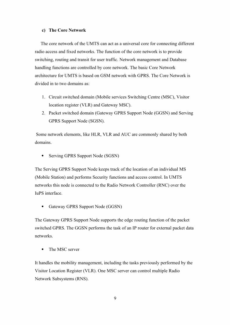
LTE SAE (System Architecture Evolution) can be divided into three different part:

UE, eNodeB and EPC (evolved packet core). Various interfaces are designed between

these entities which include Uu between UE and eNodeB, X2 between two eNodeB,

S1 between EPC and eNodeB. ENodeB has functionalities of both RNC and Node B

as previous UMTS architecture.LTE is completely IP based network.

The basic architecture contains the following network elements: LTE EUTRAN

(Evolved Universal Terrestrial Radio) and LTE Evolved Packet Core.

LTE EUTRAN

EUTRAN is the evolvement of UTRAN which was developed as a multiple access

method with a functional split between the radio access and core network in the

network architecture .It provides higher data rates, lower latency and is optimized for

packet data.

EUTRAN (Evolved Universal Terrestrial Radio) consists of Base station also called

eNodeB (an evolved UTRAN Node B). EUTRAN is responsible for complete radio

management in LTE. When UE powered is on, eNB is responsible for Radio Link

Control (RLC) layer, Radio Resource Management (RRC) and Packet Data

Convergence Protocol (PDCP). When a packet from UE arrives to eNB, eNB shall

compress the IP header and encrypt the data stream. ENB is responsible for choosing

a MME using MME selection function. The QoS is taken care by eNB as the eNB is

only entity on radio. Other functionalities include scheduling and transmission of

paging messages, broadcast messages, and bearer level rate enforcements also done

by eNB.

12

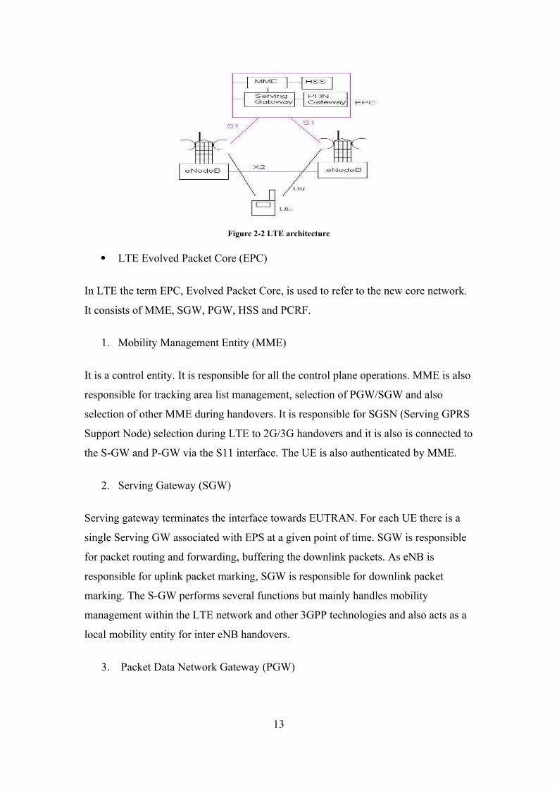
Figure 2-2 LTE architecture

LTE Evolved Packet Core (EPC)

In LTE the term EPC, Evolved Packet Core, is used to refer to the new core network.

It consists of MME, SGW, PGW, HSS and PCRF.

1. Mobility Management Entity (MME)

It is a control entity. It is responsible for all the control plane operations. MME is also

responsible for tracking area list management, selection of PGW/SGW and also

selection of other MME during handovers. It is responsible for SGSN (Serving GPRS

Support Node) selection during LTE to 2G/3G handovers and it is also is connected to

the S-GW and P-GW via the S11 interface. The UE is also authenticated by MME.

2. Serving Gateway (SGW)

Serving gateway terminates the interface towards EUTRAN. For each UE there is a

single Serving GW associated with EPS at a given point of time. SGW is responsible

for packet routing and forwarding, buffering the downlink packets. As eNB is

responsible for uplink packet marking, SGW is responsible for downlink packet

marking. The S-GW performs several functions but mainly handles mobility

management within the LTE network and other 3GPP technologies and also acts as a

local mobility entity for inter eNB handovers.

3. Packet Data Network Gateway (PGW)

13

It is connecting the user traffic from the S-GW to a trendy packet data network

(including the internet), IMS and different operator services.

4. Home Subscriber Server (HSS)

It is a central database that provides user-related and subscription-related information.

The functions of the HSS include functionalities such as mobility management, call

and session establishment support, user authentication and access authorization. In

addition the HSS holds dynamic information such as the identity of the MME to

which the user is currently attached or registered.

5. Policy Control and Charging Rules Function (PCRF)

It is responsible for policy control decision-making as well as for controlling

the flow-based charging functionalities .PCRF is also concerned with QoS

policy.

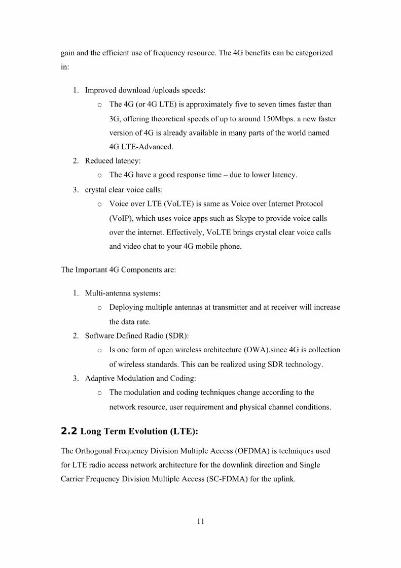
2.3 Heterogeneous Networks

Small cells are primarily added to increase capacity in hot spots with high user

demand and to fill in areas not covered by the macro network – both outdoors and

indoors. They also improve network performance and service quality by offloading

from the large macro-cells. The result is a heterogeneous network with large macro-

cells in combination with small cells providing increased bitrates per unit area.

In heterogeneous networks the cells of different sizes are referred to as macro-,

micro-, pico- and femto-cells; listed in order of decreasing base station power. The

actual cell size not only depends on the eNB power but also on antenna position, as

well as the location environment.

14

Figure 2-3 Heterogeneous Networks

2.4 Related work

Many researchers have been conducted to evaluate the performance of the LTE

handover (hard, soft, vertical, horizontal etc.) using different algorithm, parameters

and simulation. Following paragraphs reveals the method and results of each study

and finally a comparative table for these studies is listed in table (2.1).

Cheng-Chung Lin et al. has been evaluated the performance of a new handover

algorithm known as LTE Hard Handover Algorithm with Average Received Signal

Reference Power (RSRP) Constraint (LHHAARC) that can efficiently reduce the

number of handovers, minimizing the total system delay and maximizing the total

system throughput. The LHHAARC algorithm is evaluated and compared with three

well known handover algorithms using optimized handover parameters. The main

algorithm calculated as following:

RSRP¿¿ (2.3)

Where: RSRPs j (nTm ) is the RSRP received by user j from serving cell S at n-th

handover measurement period of Tm and N is the total number of periods of duration

Tm. An average RSRP of cell S received by user j (RSRP) can be calculated by a sum

of each n-th handover measurement period (Tm) up to N divided by N times. Then the

algorithm expressed in many form to provide the simulation result which have been

shown the total system delay and throughput of 4 handover algorithms in 3 speed

scenarios [2].

15

Danish Aziz et al. has been improved the performance of LTE handover through

interference coordination by presented a simple Inter Cell Interference Coordination

(ICIC) scheme and evaluated its performance on the basis of handovers in LTE. This

study has been presented that optimum HO performance can be achieved through

optimum parameters selection by finding a compromise between HO rates and

Residual Block Error Rate (BLER) for HO Command message. However, in full

high load situations this compromise still provides high Residual BLER that may lead

to high probability of radio link failures. And also provided the ICIC can overcome

the radio link failure problem without affecting the HO rates and with different

selection of HO parameters. In this study the HO algorithm expressed as:

r¿≥rns+h (2.4)

Where: r¿ Is the nth sample of filtered RSRP of any detected sector i other than the serving sector

rns Is the nth sample of filtered RSRP of the serving sector

h Is the given HOM.

The result presented the ICIC performance for the UEs moving with 30km/h with

different HOM and TTT respectively with varying filter coefficient ‘K’. It can be seen

that ICIC provides even higher gain as when the values of the HO parameters

increased [3].

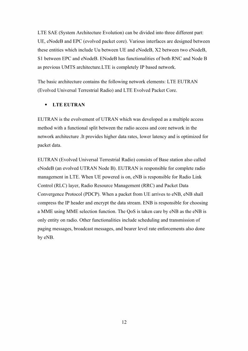
Mohammed Hicham HACHEMI et al. has been improved the real-time of spectrums

sensing in a heterogeneous LTE network. Their study leads to see the effectiveness of

t least mean square (LMS) process on the energy detection mechanism in order to

predicate the detection probability of the spectrum at (t + p) and to search other

spectrums in the surrounding by calculating the detection probability at t and to take

the right decision by comparing which have the best sensing probability. In addition,

this study allows seeing another appearance of traditional process on the triggering of

the handover. The simulation results show that the proposed algorithm attains the best

performance with the excellent precision on future spectrum sensing in real

environment contrary to the conventional HO process that depends on several

16

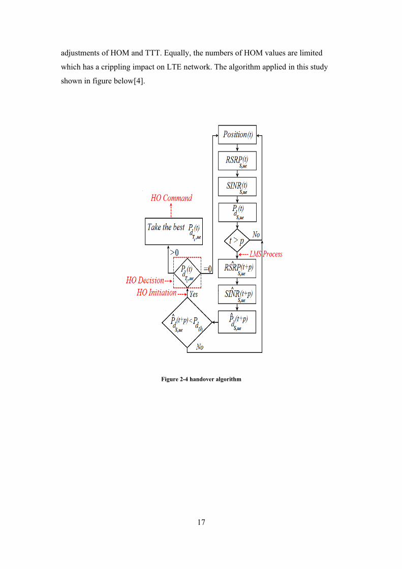
adjustments of HOM and TTT. Equally, the numbers of HOM values are limited

which has a crippling impact on LTE network. The algorithm applied in this study

shown in figure below[4].

Figure 2-4 handover algorithm

17

Table 2.2: Related work summary.

Ref. Year Simulator Networks AlgorithmsPerformance

Metrics

[2] 2011 C++ LTEAverage RSRP

ConstraintThroughput,

Delay.

[3] 2009 Matlab LTEThe filteredRSRP With

ICICError rate

[4] 2016 MatlabHeterogeneous,

LTEConventional

HandoverSNR, energy

detection

3 CHAPTER THREE – LTE Handover

18

3.1 Introduction

When a mobile user travels from one area of coverage or cell to another cell within a

call’s duration the call should be transferred to the new cell’s base station and the

Mobile phones can maintain their connections in cellular networks when they move,

this procedure called a handover (HO) or a handoff. It is needed for Mobility and

User preferences.

The handoff occur initiated when received signal level drops below a certain threshold

value, not as simple as it seems actually consider a time average of the received signal

instead of the instantaneous level.

Figure 3-5 Handover region

3.2 HANDOVER MECHANISMS

As explained earlier, handovers are used to maintain mobile client's connection in the

network, even when these clients move from a network access point to another

network access point. There are two types of handovers, horizontal and vertical. Since

the handover occurs and is supported by the same wireless technology this called

horizontal handoff and when it supported different wireless technology it called

vertical handoff. A handover process can be classified into five parts: Measurements,

processing, reporting and Decision and execution. A handover mechanism constantly

scans the air for other access points and monitors the active connection to keep the

connection. Once the service criteria aren’t fully supported anymore, or when a better

suitable network is found, then a handover procedure is started. To give a more

19

detailed view of a handover, taking a high level GSM handover as example, first the

client connects and registers with the new access point. Then the specific information

of the connection is transmitted. Only when the connection is successfully taken over,

the client disconnects from the old access point. With today’s new technologies,

vertical handovers become more popular.

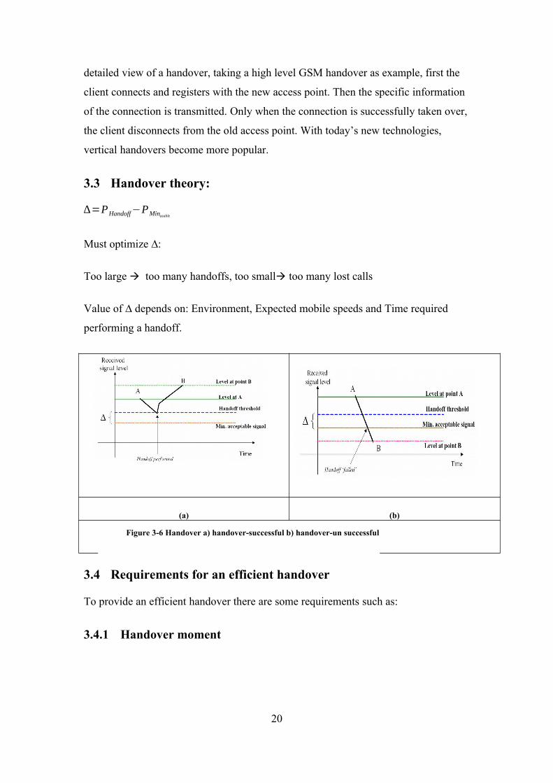
3.3 Handover theory:

∆=PHandoff−PMinusable

Must optimize ∆:

Too large too many handoffs, too small too many lost calls

Value of ∆ depends on: Environment, Expected mobile speeds and Time required

performing a handoff.

(a) (b)

3.4 Requirements for an efficient handover

To provide an efficient handover there are some requirements such as:

3.4.1 Handover moment

20

Figure 3-6 Handover a) handover-successful b) handover-un successful

The handover moment or handover location is one of the most important criteria for

an efficient handover. To supply a handover without degrading the quality of service

(QoS) the location of the handover moment should be carefully planned.

The point of a handover is at a spot where the old and the new access point have a

cross in coverage area. Outside this area there might be a lot of interference which

degrades the quality of the connection and slows the handover down. The chosen of

the handover moment at the wrong place lead to unnecessary handover.

3.4.2 Unnecessary handovers

To make the handover mechanism efficient, the number of unnecessary handovers the

must be lower. To chose the handover moment, handover mechanisms use signal

strength algorithms to calculate the distance to the access point. Measurement errors

in this process can lead to unnecessary handovers, which can lead to higher power

consumption and possible degradation of the supported QoS.

3.4.3 Handover delay

The most important criterion of the efficiency of a handover mechanism is the

duration of the handover procedure. When a handover takes too long, service

disturbance can be experienced or connections can timeout and will be lost. To

provide an efficient handover, this delay must be as short as possible. The delay

calculated from the execution of the handover algorithm until the algorithm completes

the handover procedure and the client is successfully connected to the other access

point.

3.4.4 Packet loss

No packet or data loss is almost impossible so the less packet loss a mechanism

provide, the more efficient the mechanism is. The ITU has got a QoS parameter for

the packet loss so the states of the probability for a packet loss wouldn't be more than

1 × 10–3.

3.4.5 Scalability

21

The scalability of a handover is an important requirement when implementing it into

wireless network technologies with a high increasing of mobile users.

3.4.6 Complexity

The complexity of a handover procedure is very important when talking about mobile

devices. These devices have bounded resources, if the handover procedure takes too

many resources, smaller mobile devices can’t provide the handover.

3.5 Handover techniques

Handover can be classified as: Soft handover also known as Connect-Before-Break

(CBB) and hard handover also known as Break-Before-Connect (BBC) respectively

[5].

3.5.1 Soft handover, Connect-Before-Break

Soft handover is the type of handover which connection is established before breaking

the connection. This handover is called “make before break”. In this type, a mobile at

the same time communicates with two or more cells belonging to different BSs of the

identical RNC (intra-RNC) or different RNCs (inter-RNC). When a call is in a state of

soft handover, the most excellent signal is used or all the signals can be collective to

generate a clearer copy of the signal.

Soft handover network consists of user equipment, node B, RNC, GGSN, SGSN and

Server. The GGSN include all GPRS functionality that is needed to support GSM and

UMTS packet services. The soft handover requires much more complicated signaling,

procedures and system architecture such as in the WCDMA network.

3.5.2 Hard handover, Break-Before-Connect

This handover requires a user to break the existing connection with the current cell

(serving cell) and make a new connection to the target cell. Hard handover is a type of

22

handover procedures where all the old radio links in the UE are abandoned before the

new radio links are established. In LTE only hard handover is supported, meaning that

there is a short interruption in service when the handover is performed [6].

3.6 Handover in LTE

A hybrid approach is used in LTE network. The main process of handover in LTE the

allow UE sends measurement information to network and based on those

measurements network allowed UE to move to a target cell. The process and types of

handover are provides in the following section.

3.6.1 Types of Handover in LTE network

Intra-LTE Handover: In this type source and target cells are part of the

same LTE network. There are different types of Intra-LTE handover can

be possible

Intra-MME/SGW: Handover using X2 Interface

X2 is the interface between serving eNodeB and target eNodeB in this case. When X2

interface is present then handover is completed without EPC (Evolved Packet Core)

involvement. The release of the resources at source eNodeB is triggered by target

eNodeB.

Intra-MME/SGW: Handover using S1 Interface

In this type when X2 interface is not available and source eNodeB and target eNodeB

belong to same MME/SGW then handover is carried out through S1 interface. The S-

eNB initiates the handover by sending a Handover required message over the S1-

MME reference point. The handover decisions taken by the S-eNB, the EPC do not

change.

A. Inter-LTE Handover: In this case the handover happens towards other LTE

nodes. (Inter-MME and Inter-SGW).

Inter-MME Handover

23

In this handover two MME are involved in handover, source MME and target MME.

The source MME (S-MME) is based on the source eNodeB and target MME (T-

MME) is based on target eNodeB. This handover occurs when UE moves between

two different MMEs but connected to same SGW.

Inter-MME/SGW Handover

This is same as Inter-MME but only difference is that here UE need to move from one

MME/SGW to another MME/SGW. Source eNodeB is part of one MME/SGW and

target eNodeB is in another MME/SGW.

B. Inter-RAT: Handover in this type between different radio technologies. For

example handover from LTE to WCDMA.

X2 is the name of the interface that connects one eNB to another eNB. There is a lot

of information or messages running along this interface (basically connection line).the

most common information carried over X2 is a Handover related Information .Any

data/message exchange would need some type of protocol, this protocol for

communication along X2 interface is called X2AP (X2 Application Protocol) this

protocol has many different functions like mobility management (handover

preparation and handover cancel).The step of handover shown in figure and followed

by the description.

24

Figure 3-7 LTE handover

1) A data call is established between the UE, S-eNB and the network elements.

Data packets are transferred to/from the UE to/from the network in both

directions (DL as well as UL).

2) The network sends the measurement control REQ message to the UE to set the

parameters to measure and set thresholds for those parameters. The UE sends

the measurement report to the S-eNB after it meets the measurement report

criteria communicated previously.

3) The S-eNB makes the decision to hand off the UE to a D-eNB using the

handover algorithm; each network operator could have its own handover

algorithm.

4) The S-eNB issues a handover request message to the D-eNB passing

necessary information to prepare the handover at the target side.

5) The D-eNB checks for resource availability and, if available, reserves the

resources.

6) The D-eNB sends back the handover request acknowledgement message

including a transparent container to be sent to the UE as an RRC (radio

resource control) message to perform the handover.

25

7) The S-eNB generates the RRC message to perform the handover, i.e,

RRCCONNECTION RECONFIGURATION message including the mobility

Control Information. The S-eNB performs the necessary integrity protection

and ciphering of the message and sends it to the UE.

8) The S-eNB sends the eNB status transfer message to the D-eNB.

9) The UE tries to access the D-eNB cell using the non-contention-based

Random Access Procedure. If it succeeds in accessing the target cell, it sends

the RRC connection recognition complete to the D-eNB.

10) The D-eNB sends a path switch request message to the MME to inform it that

the UE has changed cells; The MME determines that the SGW can continue to

serve the UE.

11) The MME responds to the D-eNB with a path switch REQ ACK message to

notify the completion of the handover.

12) The D-eNB now requests the S-eNB to release the resources using the X2 UE

context release message. With this, the handover procedure is complete.

3.7 LTE Hard Handover Algorithm

The LTE Hard Handover Algorithm, also known as “Power Budget Handover

Algorithm”, is a basic but effective handover algorithm consisting of two variables,

handover margin (HOM) and Time to Trigger (TTT) timer. A handover margin is a

constant variable that represents the threshold of the difference in received signal

strength between the serving and the target cells. HOM ensures the target cell is the

most appropriate cell the mobile camps on during handover.

Both HOM and TTT are used for reducing unnecessary handovers which is called

“Ping-Pong effect”. When a mobile is experiencing this effect, it is handed over from

a serving cell to a target cell and handed back to original serving cell again in a small

period of time, This effect increases the required signaling resources, decreases

system throughput, and increases data traffic delay caused by buffering the incoming

traffic at the target cell when each handover occurs.

A handover action can only be performed after the TTT condition has been satisfied.

The received signal strength is called reference signal received power (RSRP) in dB

26

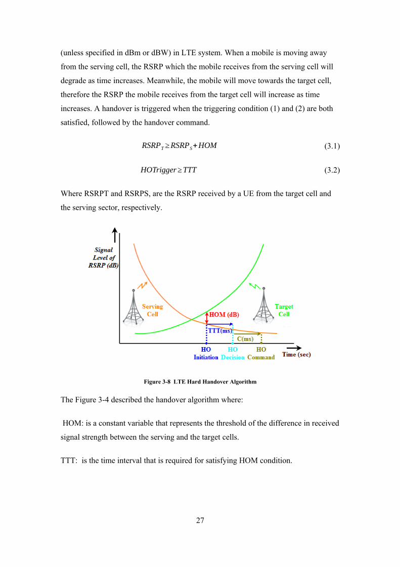
(unless specified in dBm or dBW) in LTE system. When a mobile is moving away

from the serving cell, the RSRP which the mobile receives from the serving cell will

degrade as time increases. Meanwhile, the mobile will move towards the target cell,

therefore the RSRP the mobile receives from the target cell will increase as time

increases. A handover is triggered when the triggering condition (1) and (2) are both

satisfied, followed by the handover command.

RSRPT ≥RSRPS+HOM (3.1)

HOTrigger≥TTT (3.2)

Where RSRPT and RSRPS, are the RSRP received by a UE from the target cell and

the serving sector, respectively.

Figure 3-8 LTE Hard Handover Algorithm

The Figure 3-4 described the handover algorithm where:

HOM: is a constant variable that represents the threshold of the difference in received

signal strength between the serving and the target cells.

TTT: is the time interval that is required for satisfying HOM condition.

27

HO Initiation: when equation (3.1) holds for a given TTT then the handover can be

initiated, where the UE sends the measurement report to the eNB of the serving cell.

The serving cell starts observing the incoming consecutive time slots after TTT starts.

HO decision: If the RSRP difference is less than or equal to HOM in any of the

incoming consecutive time slots, the HO process will be reset, otherwise, handover

process will be executed.

HO Command: Afterward, the preparation time is modeled as a constant protocol

delay “C” in a millisecond. When the preparation has been completed, the serving cell

sends the HO Command message to the UE.

3.8 Received Signal Strength based on TTT Window Algorithm

There are 3 steps involved in Received Signal Strength based on TTT Window

Algorithm. It collects required information during processing steps, and then performs

the comparison based on this information during decision step followed by the

execution steps.

RSSF (nTm )=BRSS (nTm )+(1−B ) RSS ( (n−1 )Tm ) (3.3)

RSSF is the filtered received signal strength (RSS, same as RSRP) measured at every

handover measurement period (Tm) where n and (n-1) is the nth and (n-1) th time

instant respectively. Is a proposed fractional number called “forgetting factor” which

can be expressed as:

B=Tu /Tm (3.4)

Where: Tu is an integer multiple of Tm. A RSS comparison will be performed based

on the following:

RSS(nTu)TS≥ RSSf (nTu)ss+HOM (3.5)

HOM is a constant threshold value, RSSF (nTu) TS and RSSF (nTu) SS are the

filtered RSS of the target sector (TS) and the filtered RSS of the serving sector (SS) at

(nTu) the interval, respectively. This algorithm tracks the RSS value from each

28

eNodeB and stores the instantaneous RSS value. Filtered RSS value at each instant is

calculated using historical data (previously filtered RSS) by applying the forgetting

factor variable [7].

3.9 Mathematical Model

The Mathematical Equations that’s used in simulation in matlabe are flow:

3.9.1 Signal to interference noise ratio (SINR)

The free space propagation model assumes the ideal propagation condition that there

is only one clear line-of-sight path between the transmitter and receiver. The

following equation presented to calculate the received signal power in free space at

distance d from the transmitter.

pr (d ) = pt G t Gr λ2

(4π )2d2 L

(3.6)

Where pt= transmitted signal power.

Gt=The antenna gains of the transmitter.

Gr= The antenna gains of the receiver.

λ= wavelength.

L=system loss.

The signal to interference is very important in mobile station and it related to data

rate, spectrum efficiency, throughput, and delay. It can be calculated as shown in

Equation (3.7).

SINR= ( pr +G ) - ( N+I ) (3.7)

Where:

SINR =Signal to interference noise ratio in (dB).

29

pr=¿Power Receiver in Mobile in (dB).

G = antenna gain.

N = noise in (db).

I = interference in (dB).

3.9.2 Data rate (DR)

Data rate: is the average number of bits per unit time (bits/second). Equation (3.8)

show the Data rate (DR).

DR= BW*M*C (3.8)

Where:

DR = data rate in (dB).

BW = Bandwidth in (Hz).

M = Number of bits per symbol (modulation index).

C = coding rate.

3.9.3 Throughput (TH)

System throughput is defined as the total number of bits correctly received by all

users and can be mathematically expressed as show in Equation (3.9)

TH=∑n=1

n

(DR(1)+DR(2)+DR(n))Bitssecond

(3.9)

Where:

TH = Throughput in (bit/sec).

SINR =Signal to interference noise ratio in (dB).

N = number of small cell.

30

3.9.4 Spectral Efficiency (SE)

It is refers to the information rate that can be transmitted over a given bandwidth in a

given system(bit/s/Hz),the equation below calculate the Spectral Efficiency (SE)

SE=DRBW

(3.10)

Where:

SE = Spectral Efficiency in (bit/s/Hz).

DR = Data rate in (bit/sec).

BW = Bandwidth in (Hz).

3.9.5 Delay transmission (DT)

System delay gives the average of the total queuing delay of all packets in the buffers

at the eNBs in the system.

System delay can be mathematically expressed as following:

DT=dataDR

Sec (3.11)

Where:

DT = Delay transmission in (sec).

Data = data transmit in (bit/sec).

DR = Data rate in (bit/sec).

The previous algorithm of the hard handover in LTE presented how the handover

process happened in a certain conditions and circumstances and when these

conditions applied the efficient handover will occur [8].

31

3.10 Simulation Model:

This section introduces some of the main elements required to develop models and explore

their behavior. One (but not the only one) of the main interests in developing models is to 'see'

how the system would behave.

Here, we use the Matlab program to implement the handover procedure using mathematical

model.

Essentially, the model operates in these stages:

1. System achieved by constant values as shown in Table 4.1 to each cell then

determines the power using mathematical equations.

2. Draw the power for each cell at distance using matlab command.

3. Determine the HOM at a specific distance.

4. Apply the hard handover algorithm.

5. Using a multiple value of TTT with a constant speed then apply the distance for each

time.

6. Determine the SINR at any time for the two cells.

7. Apply the mathematical model to determine the data rate, throughput, delay and

spectral efficiency for each signal in different time for the two cells.

8. Draw the final result using matlab command.

32

3.11 System Model Flow Chart

NO

Yes

33

END

HO Processing, calculate SNR

HO1, SNR HO2, DR, TH, SE,

HO=RSST≥RSSF+HOM

HOM=Macro_1 (y_HOM)-Macro_2 (y_HOM)

Tm=1, Tu= 0.1

Calculate Pr Macro1

BW=20, freq1=2700, freq2=2600, pt1=40, pt2=40

G=50, Lc=5

4 CHAPPTER FOUR- SIMULATION AND RESULT

This chapter presents the simulation parameters used, the results of the simulations,

and a brief discussion for each result. The simulations implemented on a Matlab

Programmer.

In the system model assumed that a user in cell edge moves from Macrocell to

another. There are two handover processes with different TTT each process provides

the result in terms of data rate, throughput, spectral efficiency, and delay of the UE.

Table 4.1: Simulation Parameters

34

4.1 Simulation Results

This section presents the simulation results:

The handovers have a great impact on the complete system performance this impact

can be realize in some parameters (delay, throughput, and spectral efficiency and data

rate as shown in the previous equations) which effect on the QoS of the network.

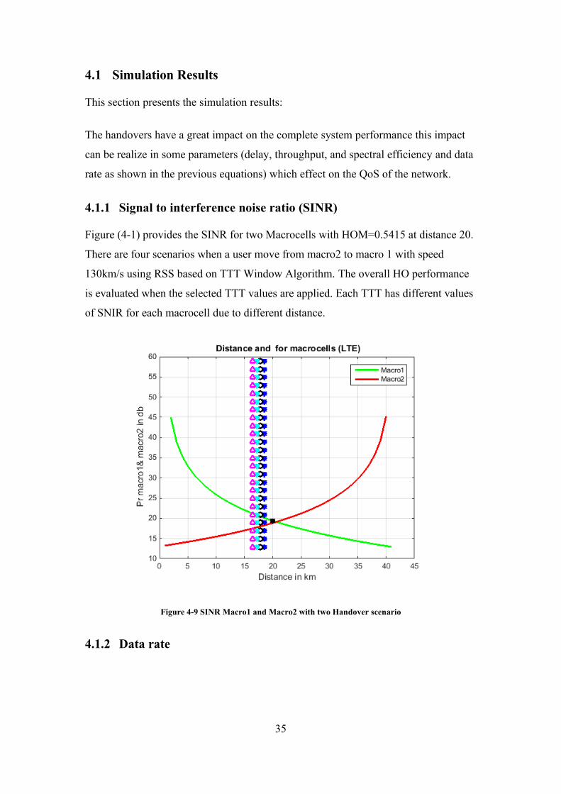
4.1.1 Signal to interference noise ratio (SINR)

Figure (4-1) provides the SINR for two Macrocells with HOM=0.5415 at distance 20.

There are four scenarios when a user move from macro2 to macro 1 with speed

130km/s using RSS based on TTT Window Algorithm. The overall HO performance

is evaluated when the selected TTT values are applied. Each TTT has different values

of SNIR for each macrocell due to different distance.

Figure 4-9 SINR Macro1 and Macro2 with two Handover scenario

4.1.2 Data rate

35

Figure (4-2) illustrates data rate for four scenarios of handovers verses TTT, the

result shows the highest data rate followed by algorithm due to use of high

Modulation and code rate when the user move to macro 1.

Figure 4-10 Data Rate of HO1&HO2

4.1.3 Accumulated Throughput

Figure (3-4) shows the entire throughput for four scenarios. Accumulated throughput

of macro1 is higher than macro2 due to increase in the data rate.

36

Figure 4-11 Accumulated Throughput

4.1.4 Spectral Efficiency

Figure (4-4) shows the spectral efficiency in different TTT, the spectral efficiency of

macro1 increasing due to the increase in data rate which use all the bandwidth.

Figure 4-12 Spectral Efficiency

4.1.5 Delay Transition

37

Figure (4-5) displays the amount of delay Transition in all scenarios verses time,

while macro2 has the higher delay on the other hand the delay of macro1 decrease and

seems to be more stable than other handover, due to the increasing of data rate.

Figure 4-13 Delay Transition

38

5 CHAPPTER FIVE – CONCLUSSION AND RECOMMENDATIONS

5.1 Conclusion

This research, in order to carry out the handover performance evaluation process,

the state of the art of handover in LTE, together with the LTE Receive signal strength

algorithm (RSS) and the LTE specifications have been studied. The operation and

performance of the simulator LTE have been investigated as well and Matlab used as

simulation part. Moreover, the handover parameters (time to trigger) have been

included in the simulator modifying the code in order to carry out the study. The

performance of the LTE handover based on the downlink RSS measurements for the

most common 3GPP scenarios has been investigated. Since the setting of HO triggers

and HOM is of primary importance for a good performance of the handover

procedure, different triggering settings for the selected parameters have been

performed with speeds mobility. The optimal settings for each scenario have been

proposed and performance evaluation has been carried out using the two scenario of

handover with two deferent TTT of handovers, SINR, throughput, Spectrum

efficiency, delay and Data Rate, the results show that the system load does affected by

adopting these parameters.

5.2 RECOMMENDATIONS

1. An interesting work that should follow this research is to investigate the

impact of this algorithm by increasing the macro-cells and divided it into small

cells.

2. However, future work might improve on the results obtained; by doing more

realistic and reliable simulation data could be achieved and presented like

result optimization.

3. More Handover network algorithms can be studied in order to enhance the

Performance for users in LTE network.

39

Reference:

[1] Brijesfverma-mobile communication- New Delhi-Indi-first adition-2009-2010[2] C.-C. Lin, K. Sandrasegaran, H. A. M. Ramli, and R. Basukala, "Optimized performance evaluation of LTE hard handover algorithm with average RSRP constraint," arXiv preprint arXiv:1105.0234, 2011.

[3] D. Aziz and R. Sigle, "Improvement of LTE handover performance through interference coordination," in Vehicular Technology Conference, 2009. VTC Spring 2009. IEEE 69th, 2009, pp. 1-5.

[4] M. H. Hachemi, M. Feham, and H. E. Adardour, "Predicting the probability of spectrum sensing with LMS process in heterogeneous LTE networks," Radioengineering, vol. 25, pp. 808-820, 2016.

[5] T. Hendrixen, "UMTS and LTE/SAE handover solutions and their comparison," in Proc. 11th Twente Student Conf. IT, 2009, pp. 1-9.

[6] H. G. Al-Qurabi, H. H. A. Al-Rubiae, and A. A. Ahmed, "Evaluation and Comparison of Soft and Hard Handovers inUniversal Mobile Telecommunication (UMTS) Networks," journal of kerbala university, vol. 8, pp. 231-243, 2010.

[7] C.-C. Lin, K. Sandrasegaran, H. A. M. Ramli, and R. Basukala, "Optimized performance evaluation of LTE hard handover algorithm with average RSRP constraint,"1105.0234, 2011.

[8] Handover Management in Highly DenseFemtocellular Networks,

MostafaZamanChowdhury and Yen Min Jang, 2013.

40

6 Appendix

Code

clc; close all,clear allDist= 0:40; %macro cell distance in km freq1_LTE = 2700;%freq in MHzfreq2_LTE = 2600;%freq in MHzBw=20; %MHztx_ht = 30;%meterrx_ht = 1.5;%meterdata=2; %the data 2k BytePT1_LTE=40; % watt %macro 1PT2_LTE=40; % watt %macro 2G1_LTE=50; %wattG2_LTE=50; %watt ;L1=5;L2=5;%Macro_1lamda1=3*10^8/(freq1_LTE*1000000)x=(PT1_LTE*G1_LTE*lamda1^2)./((4*pi)^2*(Dist./1000).^2*L1)Macro_1=10*log10(x)%plot(Macro_1)%macro_2lamda2=3*10^8/(freq2_LTE*1000000)P=(PT2_LTE*G2_LTE*lamda2^2)./((4*pi)^2*(Dist./1000).^2*L2)Macro_2=10*log10(P)%plot(Macro_2)Macro_22=Macro_2; Macro_22(1)=Macro_2(length(Macro_2));for n=2:length(Macro_2) Macro_22(n)=Macro_2((length(Macro_2))-(n-1));endMacro_2=Macro_22;figureplot(Macro_1,'g-','LineWidth',2.5)hold onplot(Macro_2,'r-','LineWidth',2.5)%plot(yhandover,margin,'k*','LineWidth',2)grid%%%%%%%%%%%%%%%%%%%%%%%%%%%%%%%%%%%%%%%%y_HOM=20; %at distance 20 HOM=Macro_1(y_HOM)-Macro_2(y_HOM);HOM_P=Macro_1(y_HOM):-1:Macro_2(y_HOM);plot(y_HOM,HOM_P,'k*','LineWidth',2)%%%%%%%%%%%%%%%%%%%%%%%%%%%%%%%%%%%%%%%%%Tm=1 % 1 ms Tu=.01 %.01ms

41

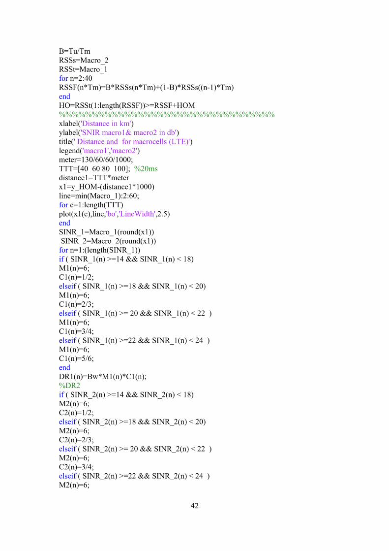
B=Tu/TmRSSs=Macro_2RSSt=Macro_1for n=2:40RSSF(n*Tm)=B*RSSs(n*Tm)+(1-B)*RSSs((n-1)*Tm)endHO=RSSt(1:length(RSSF))>=RSSF+HOM%%%%%%%%%%%%%%%%%%%%%%%%%%%%%%%%%xlabel('Distance in km')ylabel('SNIR macro1& macro2 in db')title(' Distance and for macrocells (LTE)')legend('macro1','macro2')meter=130/60/60/1000;TTT=[40 60 80 100]; %20msdistance1=TTT*meterx1=y_HOM-(distance1*1000)line=min(Macro_1):2:60;for c=1:length(TTT)plot(x1(c),line,'bo','LineWidth',2.5)endSINR_1=Macro_1(round(x1)) SINR_2=Macro_2(round(x1))for n=1:(length(SINR_1)) if ( SINR_1(n) >=14 && SINR_1(n) < 18)M1(n)=6;C1(n)=1/2;elseif ( SINR_1(n) >=18 && SINR_1(n) < 20)M1(n)=6;C1(n)=2/3;elseif ( SINR_1(n) >= 20 && SINR_1(n) < 22 )M1(n)=6;C1(n)=3/4;elseif ( SINR_1(n) >=22 && SINR_1(n) < 24 )M1(n)=6;C1(n)=5/6; endDR1(n)=Bw*M1(n)*C1(n);%DR2if ( SINR_2(n) >=14 && SINR_2(n) < 18)M2(n)=6;C2(n)=1/2;elseif ( SINR_2(n) >=18 && SINR_2(n) < 20)M2(n)=6;C2(n)=2/3;elseif ( SINR_2(n) >= 20 && SINR_2(n) < 22 )M2(n)=6;C2(n)=3/4;elseif ( SINR_2(n) >=22 && SINR_2(n) < 24 )M2(n)=6;

42

C2(n)=5/6; end;DR2(n)=Bw*M2(n)*C2(n);%caculate THTH1(1)=DR1(1)TH2(1)=DR2(1)if n >= 2 TH1(n)=TH1(n-1)+DR1(n)TH2(n)=TH2(n-1)+DR2(n)end%DelayDelay1(n)= data/(DR1(n))Delay2(n)= data/(DR2(n))%SESE1(n)=DR1(n)/BwSE2(n)=DR2(n)/Bwend;%DRfigurebar(TTT,[DR1;DR2]','grouped')gridxlabel('TTT')ylabel('Data in Mbps')title('Data rate vs TTT')legend('Data Rate Macro1','Data Rate Macro2')%Through putfigurebar(TTT,[TH1;TH2]')gridxlabel('TTT')ylabel('Throughput in Mbps')title(' Throughput vs TTT')legend('Throughput Macro1','throughput Macro2')%delayfigurebar(TTT,[Delay1;Delay2]')gridxlabel('TTT')ylabel('Delay in us ')title(' Delay vs TTT')legend('Delay Macro1','Dealy Macro2')%specralefencyfigurebar(TTT,[SE1;SE2]')gridxlabel('TTT')ylabel('Spectrum Efficiency in b/s/h')title(' Spectrum Efficiency vs TTT')

43

legend('Spectrum Efficiency Macro1','Spectrum Efficiency macro2')

44