ALTERNATE SCHEMA DIAGRAMMING METHODSDECISION SUPPORT SYSTEMSCS121: Relational DatabasesFall 2017 – Lecture 22

E-R Diagramming

¨ E-R diagramming techniques used in book are similar to ones used in industry¤ Still, plenty of variation on how schemas are diagrammed

¨ Some books use a different diagramming technique¤ Attributes are represented as

ovals attached to entity-set¤ Much harder to lay out!¤ Takes up a lot of room

¨ These methods don’t include types or other constraints

location

latitude

longitude

last_visited

description

2

Unified Modeling Language

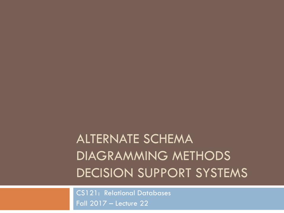
¨ A standardized set of diagrams for specifying software systems

¨ Focuses on three major areas:¤ Functional requirements:

n What is the system supposed to do?n Who may interact with the system, and what can they do?

¤ Static structure:n What subsystems comprise the system?n What classes are needed, and what do they do?

¤ Dynamic behavior:n What steps are taken to perform a given operation?n What is the flow of control through a system, and where are the

decision points?

3

UML Class Diagrams

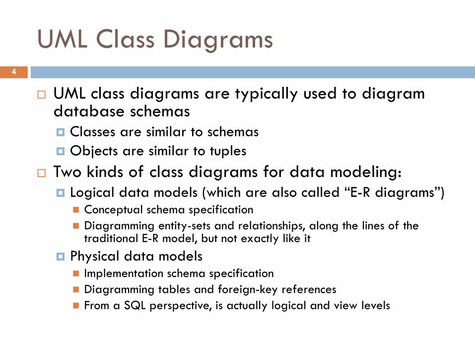
¨ UML class diagrams are typically used to diagram database schemas¤ Classes are similar to schemas¤ Objects are similar to tuples

¨ Two kinds of class diagrams for data modeling:¤ Logical data models (which are also called “E-R diagrams”)

n Conceptual schema specificationn Diagramming entity-sets and relationships, along the lines of the

traditional E-R model, but not exactly like it¤ Physical data models

n Implementation schema specificationn Diagramming tables and foreign-key referencesn From a SQL perspective, is actually logical and view levels

4

UML Data Modeling

¨ Entity-sets and tables are represented as boxes¤ First line is entity-set name¤ Subsequent lines are attributes¤ First group of attributes usually

the entity-set’s primary keyn Bolded, or marked with a *, +, or #

¨ Table diagrams oftenalso include type details

latitudelongitudedescriptionlast_visited

location

latitudelongitudedescriptionlast_visited

locationNUMERIC(8, 5)NUMERIC(8, 5)VARCHAR(1000)TIMESTAMP

5

UML Relationships

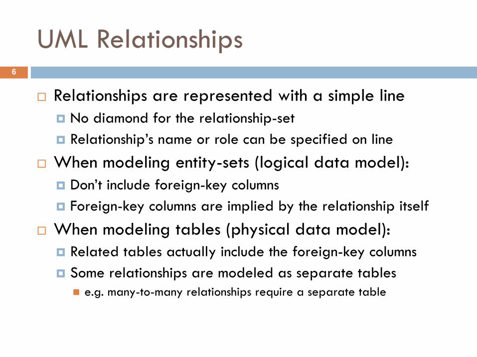
¨ Relationships are represented with a simple line¤ No diamond for the relationship-set¤ Relationship’s name or role can be specified on line

¨ When modeling entity-sets (logical data model):¤ Don’t include foreign-key columns¤ Foreign-key columns are implied by the relationship itself

¨ When modeling tables (physical data model):¤ Related tables actually include the foreign-key columns¤ Some relationships are modeled as separate tables

n e.g. many-to-many relationships require a separate table

6

UML Relationship Examples

¨ Logical data model:

¨ Physical data model:¤ (would normally include type information too)

cust_idcust_namestreetcity

customerloan_idbranch_nameamount

loancust_idloan_id

borrower

cust_idcust_namestreetcity

customerloan_idbranch_nameamount

loanborrower

7

Annotating Keys

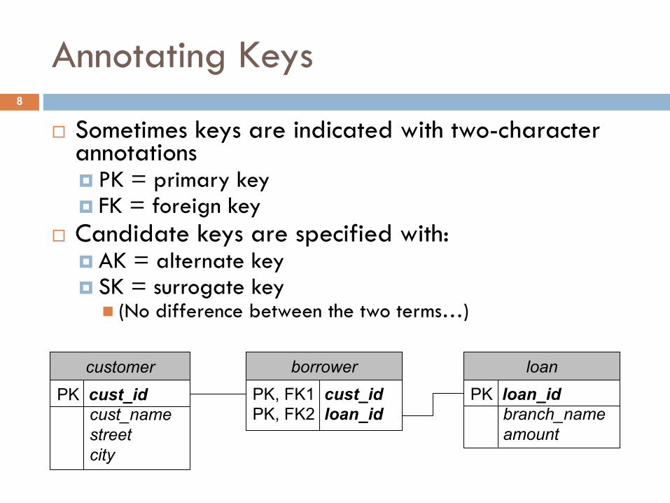
¨ Sometimes keys are indicated with two-character annotations¤ PK = primary key¤ FK = foreign key

¨ Candidate keys are specified with:¤ AK = alternate key¤ SK = surrogate key

n (No difference between the two terms…)

PK cust_idcust_namestreetcity

customerPK, FK1 cust_idPK, FK2 loan_id

borrowerPK loan_id

branch_nameamount

loan

8

Mapping Cardinalities

¨ Can specify numeric mapping constraints on relationships, just as in E-R diagrams¤ Can specify a single number for an exact quantity¤ lower..upper for lower and upper bounds¤ Use * for “many”

¨ Example:¤ Each customer is associated with zero or more loans¤ Each loan is associated with one or more customers

cust_idcust_namestreetcity

customerloan_idbranch_nameamount

loan0..*1..*

9

Information Engineering Notation

¨ Can also use Information Engineering Notation to indicate mapping cardinalities¤ Also called “crow’s foot notation”

¨ Symbols:¤ Circle means “zero”¤ Line means “one”¤ Crow’s foot means “many”

¨ Can combine symbols together¤ circle + line = “zero or one”¤ line + line = “exactly one”¤ line + crow’s foot = “one or more”

E

E

E

E2E1

E2E1

10

Barker’s Notation

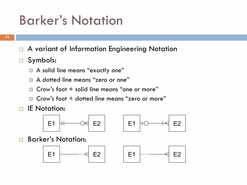
¨ A variant of Information Engineering Notation¨ Symbols:

¤ A solid line means “exactly one”¤ A dotted line means “zero or one”¤ Crow’s foot + solid line means “one or more”¤ Crow’s foot + dotted line means “zero or more”

¨ IE Notation:

¨ Barker’s Notation:

E2E1 E2E1

E2E1 E2E1

11

Examples

¨ Information Engineering notation:

¨ Barker’s notation:

cust_idcust_namestreetcity

customerloan_idbranch_nameamount

loan

cust_idcust_namestreetcity

customerloan_idbranch_nameamount

loan

12

Generalization and Specialization

¨ Can represent generalization in UML class diagrams¤ Open arrow, pointing from child to parent

¨ Can specify “disjoint” for disjoint specialization

overdraft_limitchecking

account_nobranch_namebalance

account

interest_ratesavings

disjoint

13

UML Diagramming Summary

¨ Very good idea to learn UML diagramming!¤ Used extensively in the software industry¤ You can create visual diagrams of software, and other

people will actually understand you! J¨ Significant variation in details of how data models

are diagrammed¤ Data modeling is still not yet a standard part of UML

specification¤ Good to be familiar with all major techniques

14

OLTP and OLAP Databases

¨ OLTP: Online Transaction Processing¤ Focused on many short transactions, involving a small number

of details¤ Database schemas are normalized to minimize redundancy¤ Most database applications are OLTP systems

¨ OLAP: Online Analytic Processing¤ Focused on analyzing patterns and trends in very large

amounts of data¤ Database schemas are denormalized to facilitate better

processing performance

15

Decision Support Systems

¨ Decision Support Systems (DSS) facilitate analyzing trends in large amounts of data¤ DSS don’t actually identify the trends themselves¤ Are a tool for analysts familiar with what the data means¤ Analyze collected data to measure effectiveness of current

strategies, and to predict future trends¤ Increasingly common for analysts to use data mining on a

system to identify patterns and trends, too¨ Decision support systems must provide:

¤ Specific kinds of summary data generated from the raw input data

¤ Ability to break down summary data along different dimensions, e.g. time interval, location, product, etc.

16

Decision Support Systems (2)

¨ OLAP databases are frequently part of decision support systems¤ Called data warehouses¤ Capable of storing, summarizing, and reporting on huge

amounts of data¨ Example data-sets presented via DSS:

¤ Logs from web servers or streaming media servers¤ Sales records for a large retailer¤ Banner ad impressions and click-throughs¤ Very large data sets (frequently into petabyte range)

¨ Need to:¤ Generate summary information from these records¤ Facilitate queries against the summarized data

17

DSS Databases

¨ Example: sales records for a large retailer¤ Customer ID, time of sale, sale location¤ Product name, category, brand, quantity¤ Sale price, discounts or coupons applied

¨ Billions/trillions of sales records to process¤ Summary results may also include millions/billions of rows!

¨ Could fully normalize the database schema…¤ Information being analyzed and reported on would be

spread through multiple tables¤ Analysis/reporting queries would require many joins¤ Often imposes a heavy performance penalty

¨ This approach is prohibitive for such systems!

18

Example Data Warehouses

¨ Starbucks figures from 2007:¤ 5TB data warehouse, growing by 2-3TB/year

¨ Wal-Mart figures from 2006:¤ 4PB data warehouse

¨ eBay figures from 2009:¤ Two data warehouses¤ Data warehouse 1: Teradata system

n >2PB of user data¤ Data warehouse 2: Greenplum system

n 6.5PB of user datan 17 trillion records – 150 billion new records each dayn >50TB added each day

19

Measures and Dimensions

¨ Analysis queries often have two parts:¨ A measure being computed:

¤ “What are the total sales figures…”¤ “How many customers made a purchase…”¤ “What are the most popular products…”

¨ A dimension to compute the result over:¤ “…per month over the last year?”¤ “…at each sales location?”¤ “…per brand that we carry?”

20

Star Schemas

¨ Decision support systems often use a star schema to represent data¤ A very denormalized representation of data that is well

suited to large-scale analytic processing

¨ One or more fact tables¤ Contain actual measures being analyzed and reported on

¨ Multiple dimension tables¤ Provide different ways to “slice” the data in the fact tables

¨ Fact tables have foreign-key references to the dimension tables

21

Example Star Schema

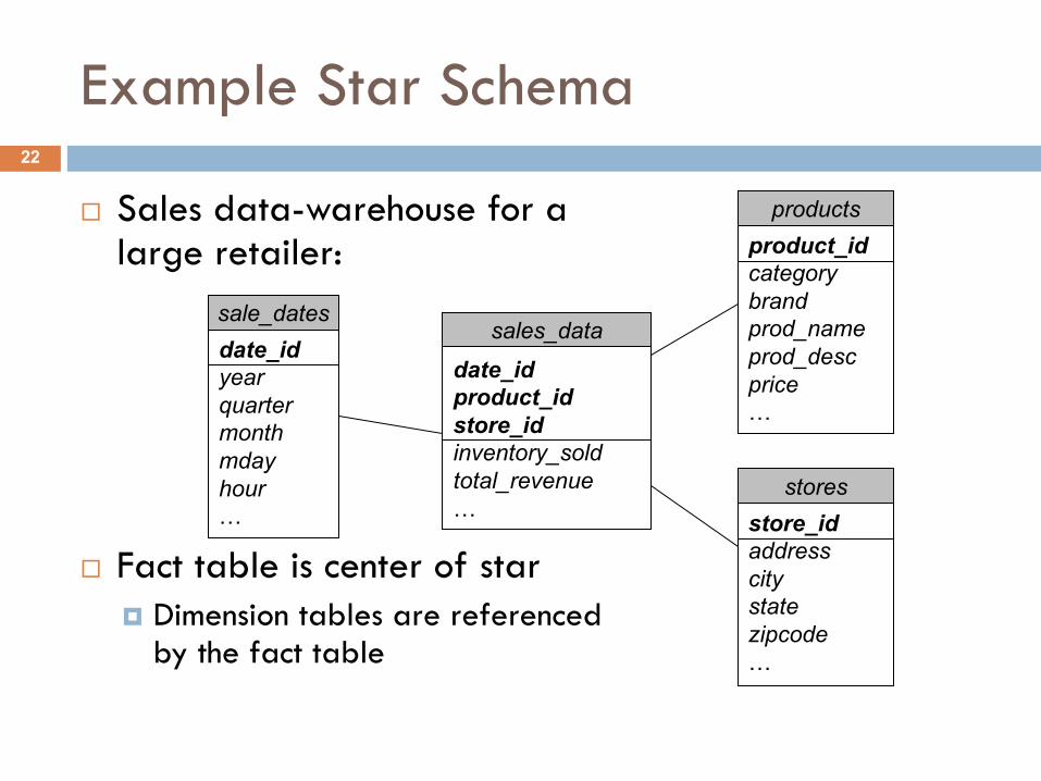
¨ Sales data-warehouse for alarge retailer:

¨ Fact table is center of star¤ Dimension tables are referenced

by the fact table

date_idproduct_idstore_idinventory_soldtotal_revenue…

sales_datadate_idyearquartermonthmdayhour…

sale_dates

product_idcategorybrandprod_nameprod_descprice…

products

store_idaddresscitystatezipcode…

stores

22

Dimensional Analysis

¨ This approach is called dimensional analysis¨ Good example of denormalizing a schema to

improve performance¤ Using a fully normalized schema will produce confusing and

horrendously slow queries

¨ Decompose schema into a fact table and several dimension tables¤ Queries become very simple to write, or to generate¤ Database can execute these queries very quickly

23

Dimension Tables

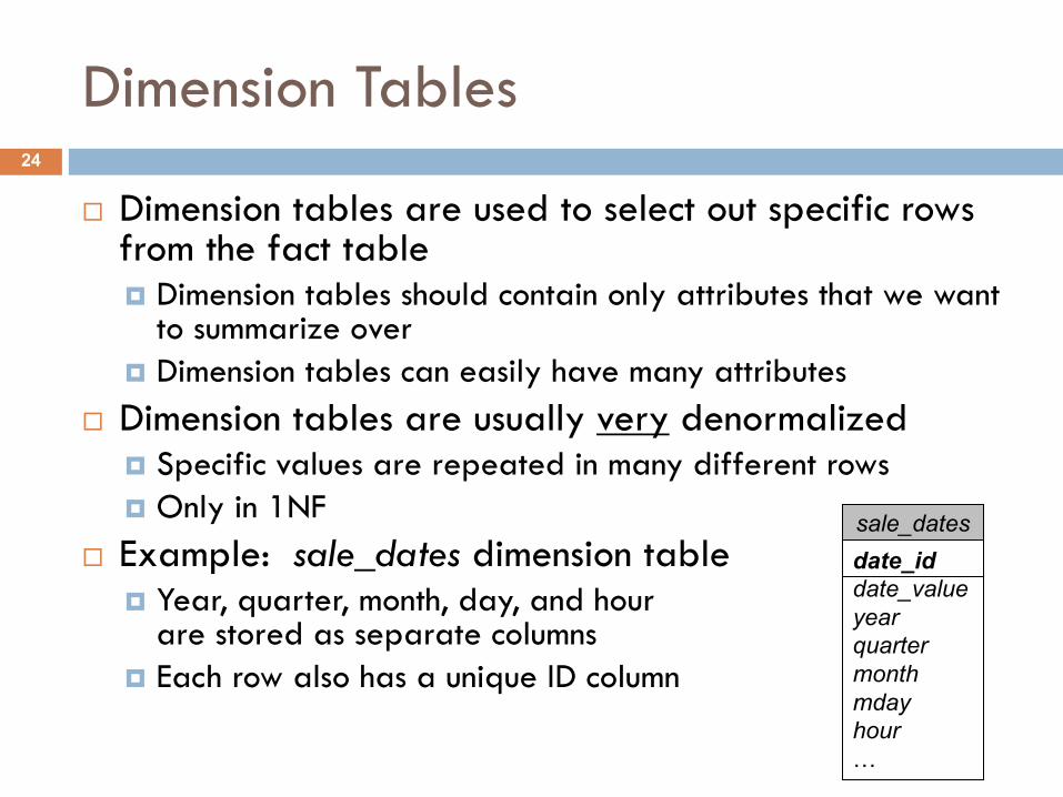
¨ Dimension tables are used to select out specific rows from the fact table¤ Dimension tables should contain only attributes that we want

to summarize over¤ Dimension tables can easily have many attributes

¨ Dimension tables are usually very denormalized¤ Specific values are repeated in many different rows¤ Only in 1NF

¨ Example: sale_dates dimension table¤ Year, quarter, month, day, and hour

are stored as separate columns¤ Each row also has a unique ID column

date_iddate_valueyearquartermonthmdayhour…

sale_dates

24

Dimension Tables (2)

¨ Dimension tables tend to be relatively small¤ At least, compared to the fact table!¤ Can be as small as a few dozen rows¤ All the way up to tens of thousands of rows, or more

n Sometimes see dimension tables in 100Ks to millions of rows for very large data warehouses

¨ Sometimes need to normalize dimension tables¤ Eliminate redundancy to reduce size of dimension table¤ Increases complexity of query formulation and processing¤ Yields a snowflake schema¤ Star schemas strongly preferred over snowflake schemas,

unless absolutely unavoidable!

25

Example Snowflake Schema

¨ Could normalize productand store details¤ Can represent more details¤ Queries become much more

complex

date_idproduct_idstore_idinventory_soldtotal_revenue…

sales_datadate_iddate_valueyearquartermonthmdayhour…

sale_dates

brand_idbrand_namesale_contact…

brands

product_idbrand_idcategory_idprod_nameprod_descprice…

products

category_idcategory_namecategory_mgr_id…

categories

region_idcitystatezipcoderegional_mgr_id…

store_regions

store_idaddressregion_id…

stores

26

Fact Tables

¨ Fact tables store aggregated values for the smallest required granularity of each dimension¤ Time dimension frequently drives this granularity

n e.g. “daily measures” or “hourly measures”

¨ Fact tables tend to have fewer columns¤ Only contains the actual facts to be analyzed¤ Dimensional data is pushed into dimension tables¤ Each fact refers to its associated dimension values using

foreign keys¤ All foreign keys in the fact table form its primary key

¨ Fact table contains the most rows, by far.¤ Well upwards of millions of rows (billions/trillions common)

27

Fact Tables (2)

¨ Not uncommon to have multiple fact tables in a data warehouse¤ Facts relating to different aspects of the enterprise, where it

doesn’t make sense to store in same table¤ Facts for a single aspect of the enterprise, but partitioned in

different waysn Used in situations where combining into a single fact table would

result in a huge, sparse fact table that is very slow to query¨ Multiple fact tables frequently share dimension tables

¤ e.g. date and/or time dimensions¤ May also have separate dimension tables only used by a

particular fact-table

28

Analytic Queries

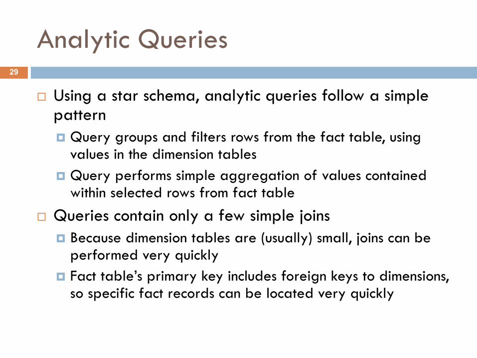
¨ Using a star schema, analytic queries follow a simple pattern¤ Query groups and filters rows from the fact table, using

values in the dimension tables¤ Query performs simple aggregation of values contained

within selected rows from fact table¨ Queries contain only a few simple joins

¤ Because dimension tables are (usually) small, joins can be performed very quickly

¤ Fact table’s primary key includes foreign keys to dimensions, so specific fact records can be located very quickly

29

Analytic Queries (2)

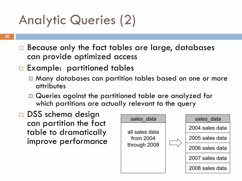
¨ Because only the fact tables are large, databases can provide optimized access

¨ Example: partitioned tables¤ Many databases can partition tables based on one or more

attributes¤ Queries against the partitioned table are analyzed for

which partitions are actually relevant to the query¨ DSS schema design

can partition the facttable to dramaticallyimprove performance

all sales datafrom 2004

through 2008

sales_data

2004 sales datasales_data

2005 sales data

2006 sales data

2008 sales data

2007 sales data

30

Slowly-Changing Dimensions

¨ Frequently, data in dimension tables changes over time¤ e.g. a “user” dimension, where some user details change

over timen e-mail address, rank/trust level within a community, last login time

¨ How do we represent slowly changing dimensions?¨ Type 1 Slowly Changing Dimensions:

¤ When a dimension value changes, overwrite the old values¤ Warehouse only maintains one row for each dimension value¤ Doesn’t track any history of changes to dimension records

n Can’t analyze facts with respect to the change history!n e.g. “How do user behaviors change, with respect to how quickly

their rank/trust level changes within their community?”

31

Slowly-Changing Dimensions (2)

¨ Type 2 Slowly Changing Dimensions:¤ Used to track change-history within a dimension¤ Rows in the dimension table are given additional attributes:

n start_date, end_date – specifies the date/time interval when the values in this dimension record are valid

n version – a count (e.g. starting from 0 or 1) indicating which version of the dimension record this row represents

n is_most_recent – a flag indicating whether this is the most recent version of the dimension record

¨ Updating a dimension record is more complicated:¤ Find current version of the dimension record (if there is one)¤ Set the end_date to “now” to indicate the old row is finished¤ Create a new dimension record with a start_date of “now”

n Fill in new dimension values; update version, is_most_recent values too

32

Good and Bad Measures

¨ Not all measures are suitable for star schemas!¨ Fact table contains partially aggregated results

¤ Analysis queries must complete aggregation, based on desired dimension and grouping aspects of query

¨ Example measures to track:¤ Quantities of each product sold

n Easy to aggregate – just sum it up¤ Average per-customer sales totals

n Fact table needs to store both the number of sales, and the total sale price, so that query can compute the average

¤ Distinct customers over a particular time intervaln Would need to store a list of actual customer IDs for each reporting

interval! Much more complex.

33

Homework 7

¨ Includes a very simple data-warehouse exercise:¤ A simple OLAP database for analyzing web logs

n Two months of access logs from NASA web server at Kennedy Space Center in Florida, from 1995

n 3.6 million records, about 300MB storage sizen Huge compared to what we have worked with so far!n Microscopic compared to most OLAP databases J

¤ Create an OLAP database scheman Star schema diagram will be provided

¤ Populate the schema from raw log data¤ Write some OLAP queries to do some simple analysis

¨ Please start this assignment early!¤ 90 students vs. 1 DB server… it could get messy… J

34