Embed Size (px)
Citation preview

Inverse Problems and Imaging doi:10.3934/ipi.2012.6.547
Volume 6, No. 3, 2012, 547–563
ALTERNATING ALGORITHMS FOR TOTAL VARIATION
IMAGE RECONSTRUCTION FROM RANDOM PROJECTIONS
Yunhai Xiao
Institute of Applied Mathematics, Henan University
Kaifeng 475004, China
Junfeng Yang
Department of Mathematics, Nanjing University
Nanjing 210093, China
Xiaoming Yuan
Department of Mathematics, Hong Kong Baptist University
Hong Kong, China
(Communicated by Hao-Min Zhou)
Abstract. Total variation (TV) regularization is popular in image reconstruc-tion due to its edge-preserving property. In this paper, we extend the alternat-
ing minimization algorithm recently proposed in [37] to the case of recovering
images from random projections. Specifically, we propose to solve the TV regu-larized least squares problem by alternating minimization algorithms based on
the classical quadratic penalty technique and alternating minimization of the
augmented Lagrangian function. The per-iteration cost of the proposed algo-rithms is dominated by two matrix-vector multiplications and two fast Fourier
transforms. Convergence results, including finite convergence of certain vari-
ables and q-linear convergence rate, are established for the quadratic penaltymethod. Furthermore, we compare numerically the new algorithms with some
state-of-the-art algorithms. Our experimental results indicate that the newalgorithms are stable, efficient and competitive with the compared ones.
1. Introduction. Variational image reconstruction plays an important role in var-ious applications, e.g., medical imaging, astronomical imaging, and transform cod-
ing. Let u ∈ Rn2
be an original n× n image, A ∈ Rm×n2
be a linear operator, andf ∈ Rm be an observation which satisfies the relationship
(1) f = N(Au) ∈ Rm,
where N(·) represents a noise corruption procedure. Given A, image reconstructionextracts u from f , which is generally ill-posed because the system could be eitherunder-determined (m < n2) as in compressive sensing or severely ill-conditioned asin deconvolution. Even when the problem is overdetermined (m > n2), f couldsuffer from outliers. Therefore, the classical least squares estimation alone does not
2000 Mathematics Subject Classification. Primary: 94A08; Secondary: 90C30.Key words and phrases. Image reconstruction, random projection, total variation, quadratic
penalty, alternating direction method.The first author is supported by NSF of China grant NSFC-11001075. The second author
is supported by NSF of China grant NSFC-11001123 and NSFC-91130007. The third author is
supported by Hong Kong General Research Fund No. 202610.
547 c©2012 American Institute of Mathematical Sciences
548 Yunhai Xiao, Junfeng Yang and Xiaoming Yuan
suffice for a faithful reconstruction. To stabilize recovery, regularization techniqueis frequently used, resulting a general reconstruction model of the form
(2) minu
Φreg(u) + µΦfid(Au− f),
where Φreg(·) promotes solution regularity such as smoothness or sparseness, Φfid(·)fits the observed data by penalizing the difference between Au and f , and µ > 0balances the two terms for minimization. The choice of Φfid(·) depends on the typeof noise, e.g., the squared `2-norm is usually used for additive Gaussian noise, whilethe `1-norm is preferred for certain non-Gaussian noise, e.g., salt-and-pepper noise.Throughout this paper, we assume that N(·) represents an additive Gaussian noisecontamination and set Φfid(·) = ‖ · ‖22. Among others, the total variation (TV)regularization has been popular ever since its introduction by Rudin, Osher andFatemi [31]. The remarkable property of TV is that it preserves edges due to thelinear penalty on differences between adjacent pixels. In this paper, we propose twoefficient algorithms for solving the following variational model
(3) minu
∑n2
i=1‖Diu‖2 +
µ
2‖Au− f‖22,
where Di ∈ R2×n2
is a local finite difference operator (with certain boundary con-ditions) at pixel i, Diu ∈ R2 denotes the discrete gradient of u at pixel i, i.e., thefinite difference of u at the ith pixel in horizontal and vertical directions, the sum∑n2
i=1 ‖Diu‖2 is a discretization of the TV of u, and A ∈ Rm×n2
. Our concentrationis the case that A is generic linear operator, which has potential applications incompressive sensing [9, 17], see, e.g., the single pixel camera architecture describedin [18].
Since the pioneering work [31], the study of numerical algorithms for solving TVmodels such as (3) has been an important subject in variational image processing,see e.g. [10, 12] and references therein. The advantage of TV regularization is thatit exploits image blocky structures and preserves edges. The superiority of TV overTikhonov regularization [34] is analyzed in [1, 15] for recovering images containingpiecewise smooth objects. Despite these advantages, it is generally challenging tosolve TV models efficiently in practice because imaging problems are usually largescale, ill-conditioned, and moreover the TV is non-smooth. Here we review someexisting approaches for solving TV models.
Early research on numerical algorithms for TV models was concentrated on
smoothed TV models, where the TV is approximated by∑n2
i=1
√‖Dix‖22 + ε with
ε > 0 small. As such, ordinary optimization methods for smooth function minimiza-tion can be applied, e.g., the time-marching scheme used in the pioneering work [31],the linearized gradient method proposed in [35, 36]. Another class of algorithms forTV problems are those based upon the iterative shrinkage/thresholding (IST) oper-ator, see e.g. [29, 21, 33]. Recently, a two-step IST algorithm was proposed in [7] bytaking advantage of the iterative information. At each iteration of IST-based algo-rithms, a TV denoising problem needs to be solved, either exactly or approximately.More recent approaches for solving TV models are based on appropriate splitting ofthe TV norm. A novel way of splitting the TV norm was proposed in [37], where theauthors utilized the quadratic penalty technique to derive an efficient alternatingminimization algorithm. This splitting of TV allows the use of a multidimensionalshrinkage operator and fast Fourier transform for deconvolution problem. By ap-plying the classical augmented Lagrangian method [27, 30], Goldstein and Osher
Inverse Problems and Imaging Volume 6, No. 3 (2012), 547–563
Alternating algorithms for image reconstruction 549
[24] derived the algorithm based on the Bregman distance [8]. Lately, the classicalalternating direction method has been applied to a set of imaging problems, see e.g.[19, 32, 2, 3, 13, 39].
We note that the time-marching scheme [31] suffers from slow convergence, whilethe IST related algorithms need to solve a TV denoising problem at each iterationwhich requires its own iterations. Although the recent advances, the efficiency of theapproaches in [37, 32] depends heavily on the problem structure. At each iterationof these algorithms, a large system of linear equations needs to be solved exactlyand efficiently, which is possible only when the matrix A preserves certain structure,e.g., A is a block-circulant matrix for deconvolution problems. However, when A isa generic linear operator, the solution of a large linear system at each iteration iscostly. In this paper, we propose efficient alternating minimization algorithms forsolving (3) where A is a generic operator and does not have structure to be explored(see also [11, 20]). Note that the case with generic A has important applicationsin the emerging methodology of compressive sensing. For example, it was shownin [9] that TV regularization is able to recover piecewise constant images exactlyfrom very few Fourier measurements. Exact recoverability of sparse and piecewiseconstant (sparse gradient) signals is also attainable for a large class of randommatrices with less rows than columns, see e.g., [41]. Another popular application isthe TV-regularized CT-image reconstruction, where A is a partial Radon transformmatrix which depends on the location and direction of each beamlet [16].
The main contribution of this paper is to present two efficient alternating mini-mization algorithms for solving (3), one is based on the classical quadratic penaltymethod, and the other is based on the alternating minimization of the augmentedLagrangian function (which is known as alternating direction method or ADM, [22]).For the first algorithm, we establish finite convergence of certain variables and q-linear convergence rate under reasonable assumptions. For the second algorithm,we show that its convergence can be guaranteed by results in the literature. We alsocompare these new algorithms with some state-of-the-art algorithms numerically.
In the rest of this paper, the inner product of two vectors will be denoted by
〈u, v〉. Without misleading, we let ‖ · ‖ = ‖ · ‖2 and∑i =
∑n2
i=1. Additionalnotation will be introduced when it occurs.
2. An alternating minimization algorithm. The task of this section is to de-velop an alternating minimization algorithm for solving (3) based on the classicalquadratic penalty method.
By introducing auxiliary variables wi ∈ R2 for each i and letting
w = (w1, . . . ,wn2) ∈ R2×n2
, we can easily reformulate (3) into
(4) minu,w
{∑i‖wi‖+
µ
2‖Au− f‖2 : wi = Diu, i = 1, 2, . . . , n2
}.
To deal with constraints, we apply the quadratic penalty method and approximate(4) by
(5) minu,w
∑i
(‖wi‖+
β
2‖wi −Diu‖2
)+µ
2‖Au− f‖2,
where β > 0 is a sufficiently large penalty parameter. This splitting was firstintroduced for deconvolution problem in [37], and then was extended to deal withcross-channel image deconvolution in [38] and impulsive noise elimination based ona TVL1 model in [40].
Inverse Problems and Imaging Volume 6, No. 3 (2012), 547–563
550 Yunhai Xiao, Junfeng Yang and Xiaoming Yuan
2.1. Alternating minimization. The advantage of (5) is that it permits alter-nating minimization. It is easy to see that, for fixed u = uk, the minimization of(5) with respect to w reduces to the following two-dimensional problems
(6) minwi∈R2
‖wi‖+β
2‖wi −Diu
k‖2, i = 1, 2, . . . , n2,
for which the unique minimizers are given by the two-dimensional shrinkage formu-las
(7) wk+1i = max
{‖Diu
k‖ − 1
β, 0
}Diu
k
‖Diuk‖, i = 1, . . . , n2,
where the convention 0 · (0/0) = 0 is followed. On the other hand, for fixed w =wk+1, the minimization of (5) with respect to u is a least squares problem of theform
(8) minu
∑i‖wk+1
i −Diu‖2 +µ
β‖Au− f‖2.
The normal equations of (8) are given by
(9)
(∑iD>i Di +
µ
βA>A
)u =
∑iD>i w
k+1i +
µ
βA>f.
It is well-known that, under the periodic boundary condition for u,∑iD>i Di is
a block-circulant matrix and can be diagonalized by the two-dimensional Fouriermatrix. However, the matrix A>A does not have circulant structure for generalrandom matrix A. Therefore, the exact solution of (9) is costly and should beavoided, which will be addressed in the following.
To avoid solving the linear system (9), similar with the approach in [25, 14], ateach iteration we linearize ‖Au − f‖2 at the current point uk and add a proximalterm, resulting the following approximation problem to (8):
minu
∑i‖wk+1
i −Diu‖2 +2µ
β
(1
2‖Auk − f‖2 + g>k (u− uk) +
1
2τ‖u− uk‖2
),
(10)
where gk = A>(Auk − f) is the gradient of 12‖Au − f‖2 at uk, and τ > 0 is a
parameter. Simple manipulations show that (10) is equivalent to
(11) minu
∑i‖wk+1
i −Diu‖2 +µ
βτ‖u− (uk − τgk)‖2.
The normal equations of (11) are given by
(12)
(∑iD>i Di +
µ
βτI
)u =
∑iD>i w
k+1i +
µ
βτ(uk − τgk).
Under the periodic boundary conditions for u, the coefficient matrix in (12) can bediagonalized by the two dimensional Fourier matrix. Consequently, the solution of(12) can be accomplished by two fast Fourier transforms or FFTs (including oneinverse FFT). To sum up, our alternating minimization algorithm for solving theapproximation problem (5) is as follows.
Algorithm 2.1. Input f , A and µ, β, τ > 0. Initialize u0 and k = 0.
While “not converged”, Do1) Compute wk+1 according to (7).2) Compute uk+1 according to (12) and let k = k + 1.
End Do
Inverse Problems and Imaging Volume 6, No. 3 (2012), 547–563
Alternating algorithms for image reconstruction 551
The implementation details of Algorithm 2.1, such as choices of parameters andstopping criterion, will be addressed in Section 4. In the following we analyze itsconvergence properties.
2.2. Convergence analysis. The purpose of this subsection is to establish con-vergence properties of Algorithm 2.1 for a fixed β > 0. For convenience, we firstdefine some notation.
We let the corresponding global finite difference operators in horizontal and verti-cal directions be D(1) and D(2), respectively, which are n2×n2 matrices. For simpli-
fication, we let D = ((D(1))>, (D(2))>)> ∈ R2n2×n2
, and thus∑iD>i Di = D>D.
For j = 1, 2, we let w>j be the the j-th row of w = [w1, . . . ,wn2 ] ∈ R2×n2
and
w = (w1;w2) , (w>1 , w>2 )> ∈ R2n2
. Since w and w are the same set of variableswith different ordering, in the following we use either w or w subject to convenience.For fixed β > 0, the 2-dimensional shrinkage operator s : R2 → R2 is defined as
(13) s(α) , α− PB(α) = max
{‖α‖ − 1
β, 0
}α
‖α‖,
where PB(·) : R2 → R2 is the projection onto the closed ball B , {α ∈ R2 : ‖α‖ ≤1/β}, and the convention 0 · (0/0) = 0 is followed. For vectors u, v ∈ RN , N ≥ 1,we define S(u; v) : R2N → R2N by
S(u; v) = (s(α1)>, . . . , s(αN )>)>, where αi = (ui, vi)>,
i.e., S applies the 2-dimensional shrinkage to each pair (ui, vi)>, for i = 1, 2, . . . , N .
From the definition of s(·), it is easy to see that (7) can be rewritten as wk+1i =
s(Diuk). The following result shows that the operator s is non-expansive.
Lemma 2.1. For any a, b ∈ R2, it holds that
‖s(a)− s(b)‖2 ≤ ‖a− b‖2 − ‖PB(a)− PB(b)‖2.
Furthermore, if ‖s(a)− s(b)‖ = ‖a− b‖, then s(a)− s(b) = a− b.
The proof of Lemma 2.1 can be found, e.g., in [37]. To establish the convergenceof Algorithm 2.1, we need the following technical assumption.
Assumption 2.1. N (A) ∩N (D) = {0}, where N (·) represents the null space of amatrix.
Since the objective function in (5) is convex, bounded below, and coercive (i.e.,it goes to infinity as ‖(w, u)‖ → ∞), it has at least one minimizer (w∗, u∗) whichmust satisfy
(14)
{w∗ = S(D(1)u∗;D(2)u∗) = S(Du∗),(D>D + µ
βA>A)u∗ = D>w∗ + µ
βA>f.
By using the shrinkage operator, we can rewrite the iteration of Algorithm 2.1 as
(15)
{wk+1 = S(D(1)uk;D(2)uk) = S(Duk),(D>D + µ
βτ I)uk+1 = D>wk+1 + µβτ (uk − τgk).
In the following, we show that (15) converges to (14). For the convenience ofanalysis, we define
M = D>D +µ
βA>A, H = D>D +
µ
βτI and T = I − τA>A.
Inverse Problems and Imaging Volume 6, No. 3 (2012), 547–563
552 Yunhai Xiao, Junfeng Yang and Xiaoming Yuan
Assumption 2.1 ensures the non-singularity of M , while H−1 is always well de-
fined. Simple manipulation shows that H −M = η2T with η ,√
µβτ . With these
definitions, (14) and (15) can be, respectively, simplified as
(16)
w∗ = S(Du∗),v∗ = ηTu∗ + ητA>f,Hu∗ = D>w∗ + ηv∗,
and
(17)
wk+1 = S(Duk),vk+1 = ηTuk + ητA>f,Huk+1 = D>wk+1 + ηvk+1.
To further simplify the above equations, we define
h(w; v) = DH−1
(DηI
)>(wv
)and
p(w; v) = ηTH−1
(DηI
)>(wv
).
Hence, the solution and iteration systems in (16) and (17) can be, respectively,rewritten as
(18)
w∗ = S ◦ h(w∗; v∗),v∗ = p(w∗; v∗) + ητA>f,Hu∗ = D>w∗ + ηv∗,
and
(19)
wk+1 = S ◦ h(wk; vk),vk+1 = p(wk; vk) + ητA>f,Huk+1 = D>wk+1 + ηvk+1,
where “◦” denotes operator composition. Furthermore, we let
q(w; v) =
(S ◦ h(w; v)p(w; v)
)+
(0
ητA>f
).
Then (18) and (19) become {(w∗; v∗) = q(w∗; v∗),Hu∗ = D>w∗ + ηv∗,
and {(wk+1; vk+1) = q(wk; vk),Huk+1 = D>wk+1 + ηvk+1.
Now we present an important lemma that will be used for convergence analysisof Algorithm 2.1. Its proof is given in Appendix A.
Lemma 2.2. q(w; v) is non-expansive, i.e., for any (w1; v1), (w2; v2) ∈ R2n2×n2
,it holds that
(20) ‖q(w1; v1)− q(w2; v2)‖ ≤∥∥∥∥ w1 − w2
v1 − v2
∥∥∥∥ ,and equality holds in (20) if and only if
q(w1; v1)− q(w2; v2) =
(w1 − w2
v1 − v2
).
Inverse Problems and Imaging Volume 6, No. 3 (2012), 547–563
Alternating algorithms for image reconstruction 553
Corollary 1. Suppose (w∗; v∗) is a fixed point of q, i.e., (w∗; v∗) = q(w∗; v∗). Thenfor any (w; v) it holds
‖q(w; v)− q(w∗; v∗)‖ < ‖(w; v)− (w∗; v∗)‖,unless (w; v) is also a fixed point of q(·; ·).
Using exactly the same arguments as [37, Theorem 3.4], we can prove the follow-ing theorem. Due to this similarity, we omit the proof.
Theorem 2.3. Under Assumption 2.1, for any fixed β > 0 and 0 < τ <2/λmax(A>A), where λmax(A>A) denotes the spectral radius of A>A, the sequence{(wk, uk)} generated by Algorithm 2.1 from any starting point (w0, u0) converges toa solution (w∗, u∗) of (5).
For each i, we let hi(w; v) = DiH−1(D>w + ηv) : R3n2 → R2,
L = {i : ‖Diu∗‖ ≡ ‖hi(w∗, v∗)‖ ≤ 1/β} and E = {1, . . . , n2} \ L.(21)
Furthermore, we let
(22) ω = min{1/β − ‖Diu∗‖ : i ∈ L} > 0.
It is theoretically interesting that the iterates produced by Algorithm 2.1 will con-verge in a finite number of steps for certain variables, though this behavior may notbe easily observable in practical experiments. In fact, we have the following finiteconvergence result for the variables {wi : i ∈ L}.
Theorem 2.4. Suppose {(wk, uk)} generated by Algorithm 2.1 converges to (w∗, u∗).Then, we have wk
i ≡ w∗i = 0, ∀ i ∈ L, after a finite number of iterations.
Proof. From Lemma 2.1, for each i, it holds
‖wk+1i −w∗i ‖ =‖s ◦ hi(wk; vk)− s ◦ hi(w∗; v∗)‖
≤‖hi(wk; vk)− hi(w∗; v∗)‖.(23)
Suppose that at iteration k there exist at least one index i ∈ L such that wk+1i =
s ◦ hi(wk; vk) 6= 0. Then ‖hi(w∗; v∗)‖ ≤ 1/β, ‖hi(wk; vk)‖ > 1/β, and w∗i =s ◦ hi(w∗; v∗) = 0. Therefore,
‖wk+1i −w∗i ‖ = ‖s ◦ hi(wk; vk)‖2 = (‖hi(wk; vk)‖ − 1/β)2
≤ ‖hi(wk; vk)− hi(w∗; v∗)‖2 − ω2.(24)
Combining (22) with (24), we obtain∥∥∥∥ wk+1 − w∗vk+1 − v∗
∥∥∥∥2
≡∑i
‖wk+1i −w∗i ‖2 + ‖vk+1 − v∗‖2
≤∑i
‖hi(wk; vk)− hi(w∗; v∗)‖2 − ω2 + ‖vk+1 − v∗‖2
=‖h(wk; vk)− h(w∗; v∗)‖2 − ω2 + ‖p(wk; vk)− p(w∗; v∗)‖
≤∥∥∥∥ wk − w∗vk − v∗
∥∥∥∥2
− ω2,
where the second “≤” comes from the non-expansiveness of
φ(w; v) =
(h(w; v)p(w; v)
),
Inverse Problems and Imaging Volume 6, No. 3 (2012), 547–563
554 Yunhai Xiao, Junfeng Yang and Xiaoming Yuan
which can be easily derived. Therefore, the number of iterations k with wk+1i 6= 0
does not exceed
1
ω2
∥∥∥∥ w0 − w∗v0 − v∗
∥∥∥∥2
,
which completes the proof.
Theorem 2.5. Under the conditions of Theorem 2.3, the sequence {uk} generatedby Algorithm 2.1 converges to u∗ q-linearly.
Proof. From the iteration formulae for u and (w; v), there holds
(25) uk+1 − u∗ = H−1
(DηI
)>(wk+1 − w∗vk+1 − v∗
),
and ∥∥∥∥ wk+1 − w∗vk+1 − v∗
∥∥∥∥2
= ‖q(wk; vk)− q(w∗; v∗)‖2
≤∥∥∥∥ D(uk − u∗)ηT (uk − u∗)
∥∥∥∥2
=
∥∥∥∥R( wk − w∗vk − v∗
)∥∥∥∥2
,(26)
where R = (D; ηT )H−1(D; ηI)>. Considering the finite convergence of wi, i ∈ L,we have ∥∥∥∥ wk+1
E − w∗Evk+1 − v∗
∥∥∥∥2
≤ ρ((R>R)EE)
∥∥∥∥ wkE − w∗Evk − v∗
∥∥∥∥2
,
where (R>R)EE is a sub-matrix of R>R ∈ R3n2×3n2
formed by deleting certain rowsand corresponding columns with indexes in ∪i∈L{i, i+n2}. Multiplying (D; ηT ) onboth sides of (25), we get
‖uk+1 − u∗‖2D>D+η2T 2 =
(wk+1 − w∗vk+1 − v∗
)>R>R
(wk+1 − w∗vk+1 − v∗
)≤ ρ((R>R)EE)
∥∥∥∥ wk+1 − w∗vk+1 − v∗
∥∥∥∥2
≤ ρ((R>R)EE)‖uk − u∗‖2D>D+η2T 2 ,
where the first “≤” is due to the finite convergence of wi, i ∈ L, and the second oneis because (26). This implies that {uk} converges q-linearly.
3. An inexact alternating direction method. It is well known that problem (5)well approximates (3) only when β is sufficiently large. In practice, it is generallydifficult to determine theoretically how large the value of β should be in orderto attain a given accuracy. In the following, we present an inexact ADM, whichconverges to a solution of (3) with any fixed β > 0. For this purpose, we considerthe augmented Lagrangian function of (4):
(27) L(w, u, λ) ,∑
i
(‖wi‖ − λ>i (wi −Diu) +
β
2‖wi −Diu‖2
)+µ
2‖Au− f‖2,
where, for each i, λi ∈ R2 is the Lagrangian multiplier attached to wi = Diu. Theclassical ADM approach [22, 23] is a variant of the augmented Lagrangian method
Inverse Problems and Imaging Volume 6, No. 3 (2012), 547–563
Alternating algorithms for image reconstruction 555
[27, 30] for convex optimization problems with separable structures such as (4).Given (uk, λk), the ADM iterates as follows
wk+1 = arg minw L(w, uk, λk),uk+1 = arg minu L(wk+1, u, λk),
λk+1i = λki − β(wk+1
i −Diuk+1), ∀ i.
(28)
The advantages of the ADM framework (28) are: i) it exploits the separable struc-ture of the objective function in (4); and ii) the value of β can be fixed to ensurethe convergence of ADM. It is easy to see that the w-subproblem in the ADMframework (28) is equivalent to
minwi∈R2
‖wi‖+β
2‖wi − (Diu
k + λki /β)‖2, i = 1, 2, . . . , n2,
the solutions of which are given by
(29) wk+1i = max
{‖Diu
k + λki /β‖ −1
β, 0
}Diu
k + λki /β
‖Diuk + λki /β‖, i = 1, 2, . . . , n2.
However, the u-subproblem in the ADM framework (28) is expensive to solve dueto the same reason as for (9). We adopt the same linearization technique andapproximate the u-subproblem by
minu
∑i
(−(λki )>(wk+1
i −Diu) +β
2‖wk+1
i −Diu‖2)
+µ
2τ‖u− (uk − τgk)‖2,
(30)
where gk = A>(Auk − f). It is easy to show that the normal equations of (30) areof the form
(31)
(D>D +
µ
βτI
)u = D>
(wk+1 − λk
β
)+
µ
βτ(uk − τgk).
Under the periodic boundary conditions, the exact solution uk+1 of (31) can beattained by two FFTs. Finally, λ is updated as in (28), or equivalently
(32) λk+1 = λk − β(wk+1 −Duk+1).
To sum up, we have the following inexact ADM algorithm for solving (4).
Algorithm 3.1. Input f , A and µ, β, τ > 0. Initialize u0 and k = 0.
While “not converged”, Do1) Compute wk+1 according to (29).2) Compute uk+1 according to (31).3) Update λk via (32) and set k = k + 1.
End Do
Now, we discuss the convergence of the proposed inexact ADM. From the abovediscussions, we see that the only difference between Algorithm 3.1 and the ADM(28) lies in the solution of the u-subproblem. To avoid the prohibitive cost on solvinga large linear system at each iteration, we adopted the linearization and proximaltechniques. It is easy to show that the approximation problem (30) is equivalent to
(33) minuL(wk+1, u, λk) +
µ
2‖u− uk‖2S ,
where S = 1τ I − A>A and ‖v‖2S = v>Sv. Therefore, Algorithm 3.1 is actually
a proximal inexact ADM, in which one subproblem is solved exactly, while the
Inverse Problems and Imaging Volume 6, No. 3 (2012), 547–563

556 Yunhai Xiao, Junfeng Yang and Xiaoming Yuan
other is solved approximately using the proximal formulation (33). Note that amore general proximal inexact ADM has been studied in [26] in the context ofmonotone variational inequality, where both subproblems are allowed to be solvedapproximately by using proximal method like (33). Therefore, the convergence ofAlgorithm 3.1 can be guaranteed by the results in [26] provided that S � 0 issatisfied.
From [26, Theorem 4], we have the following convergence result for Algorithm3.1.
Theorem 3.1. Under Assumption 2.1, for any β > 0, the sequence {(wk, uk)}generated by Algorithm 3.1 from any starting point (w0, u0) converges to a solutionof (4) provided that 0 < τ < 1/λmax(A>A).
4. Numerical results. In this section, we report numerical results to illustratethe performance of the proposed algorithms. For convenience, the proposed algo-rithms are named as Fast Total Variation image reconstruction from CompressiveSensing measurements or FTVCS. Specifically, we refer to Algorithms 2.1 and 3.1as FTVCS-v1 and FTVCS-v2, respectively. We performed two classes of numeri-cal experiments. In the first class, we compare the performance of FTVCS-v1 andFTVCS-v2, while in the second class we compare FTVCS-v2 with several state-of-the-art algorithms to illustrate its efficiency and stability. All experiments were per-formed under Windows XP Professional Service Pack 3 and MATLAB v7.8 (R2009a)running on a PC with an Intel Core 2 Quad CPU at 2.83 GHz and 3 GB of memory.
4.1. Test on FTVCS-v1 and FTVCS-v2. In this experiment, we used a randommatrix A with independent identically distributed Gaussian entries and tested theShepp-Logan phantom image, which has been widely used in simulations for TVmodels. Due to storage limitation, we tested the image size 64×64 and selected 30%samples uniformly at random. Besides, we added Gaussian noise of mean zero andstandard deviation σ = 0.001. Similar as in FTVd [37], we implemented FTVCS-v1with a continuation scheme on β to speed up convergence. Specifically, we tested theβ-sequence {24, 25, 26, 27} and used the warm-start technique. In FTVCS-v2, thevalue of β was fixed to be 8, which was determined based on experimental results.The algorithmic parameter τ was set to be 1/λmax(A>A) for both algorithms, andthe model parameter µ was set to be 200. Both algorithms were terminated whenthe relative change between successive iterates fall below 10−3, i.e.,
(34) ‖uk − uk−1‖ ≤ 10−3‖uk−1‖.We measured the quality of reconstruction by relative error (RE) to the originalimage u, i.e.,
RE = ‖u− u‖/‖u‖ × 100%,
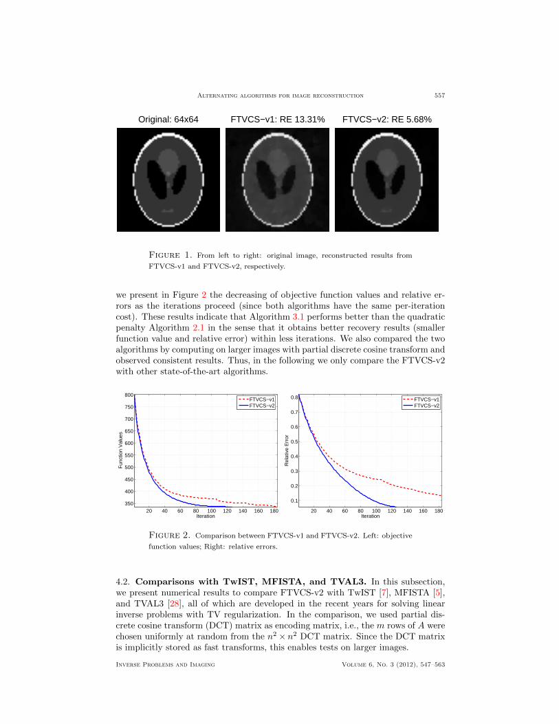
where u and u are, respectively, the original and the recovered images. The recon-struction results from both algorithms are presented in Figure 1.
It can be seen from Figure 1 that both algorithms produced faithful recoveryresults. We note that, for the Phantom image, the length of edges grows linearlywhile the number of pixels grows quadratically as n increases. Therefore, the spar-sity ratio (defined by spr = #{i : ‖Diu‖ 6= 0}/n2) of the Phantom image becomesbigger for smaller n. Specifically, for the tested 64 × 64 Phantom image, we havespr = 12.26%, while the sample ratio is only 30%, which together with the presenceof Gaussian noise explain why the recovered image by FTVCS-v2 has relative erroras large as 5.68%. To closely examine the convergence behavior of both algorithms,
Inverse Problems and Imaging Volume 6, No. 3 (2012), 547–563
Alternating algorithms for image reconstruction 557
Original: 64x64 FTVCS−v1: RE 13.31% FTVCS−v2: RE 5.68%
Figure 1. From left to right: original image, reconstructed results from
FTVCS-v1 and FTVCS-v2, respectively.
we present in Figure 2 the decreasing of objective function values and relative er-rors as the iterations proceed (since both algorithms have the same per-iterationcost). These results indicate that Algorithm 3.1 performs better than the quadraticpenalty Algorithm 2.1 in the sense that it obtains better recovery results (smallerfunction value and relative error) within less iterations. We also compared the twoalgorithms by computing on larger images with partial discrete cosine transform andobserved consistent results. Thus, in the following we only compare the FTVCS-v2with other state-of-the-art algorithms.
20 40 60 80 100 120 140 160 180350
400
450
500
550
600
650
700
750
800
Iteration
Fun
ctio
n V
alue
s
FTVCS−v1FTVCS−v2
20 40 60 80 100 120 140 160 180
0.1
0.2
0.3
0.4
0.5
0.6
0.7
0.8
Iteration
Rel
ativ
e E
rror
FTVCS−v1FTVCS−v2
Figure 2. Comparison between FTVCS-v1 and FTVCS-v2. Left: objective
function values; Right: relative errors.
4.2. Comparisons with TwIST, MFISTA, and TVAL3. In this subsection,we present numerical results to compare FTVCS-v2 with TwIST [7], MFISTA [5],and TVAL3 [28], all of which are developed in the recent years for solving linearinverse problems with TV regularization. In the comparison, we used partial dis-crete cosine transform (DCT) matrix as encoding matrix, i.e., the m rows of A werechosen uniformly at random from the n2 × n2 DCT matrix. Since the DCT matrixis implicitly stored as fast transforms, this enables tests on larger images.
Inverse Problems and Imaging Volume 6, No. 3 (2012), 547–563
558 Yunhai Xiao, Junfeng Yang and Xiaoming Yuan
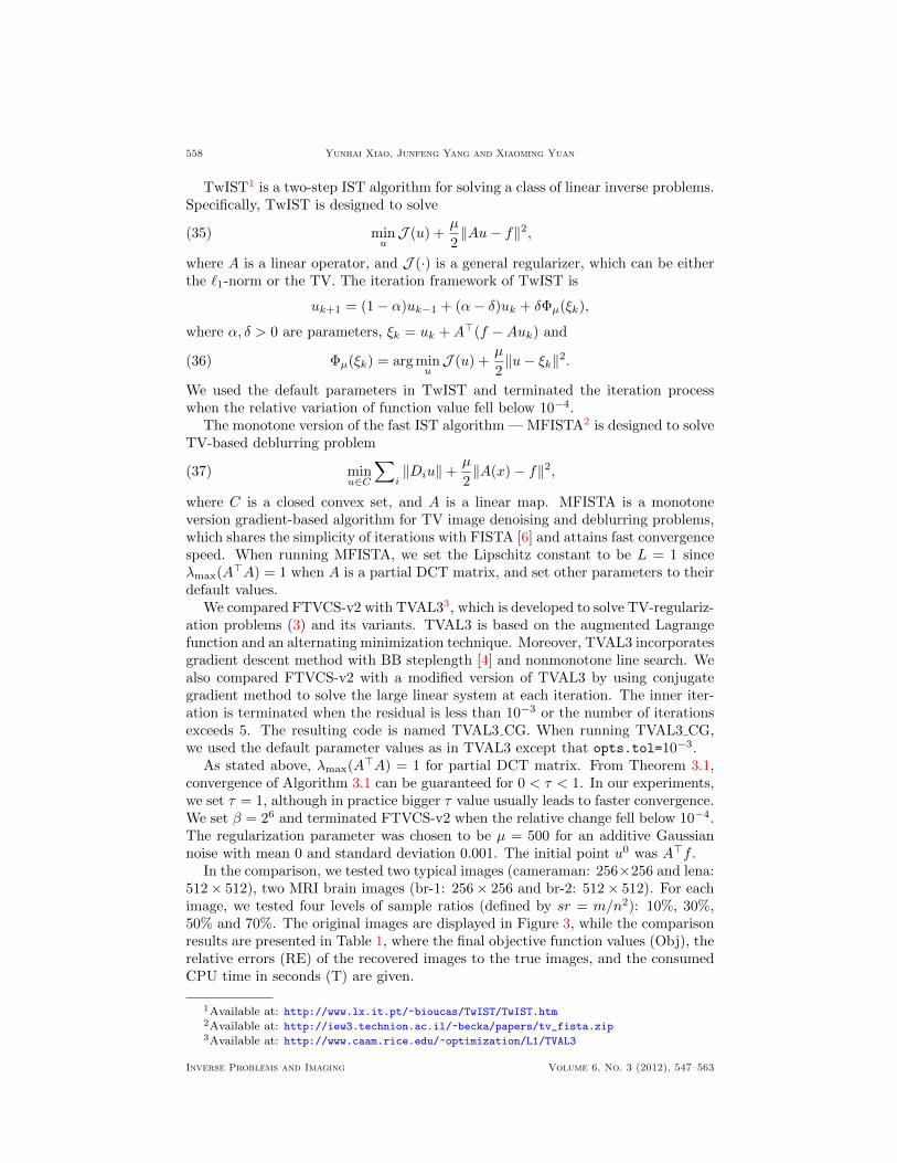
TwIST1 is a two-step IST algorithm for solving a class of linear inverse problems.Specifically, TwIST is designed to solve
(35) minuJ (u) +
µ
2‖Au− f‖2,
where A is a linear operator, and J (·) is a general regularizer, which can be eitherthe `1-norm or the TV. The iteration framework of TwIST is
uk+1 = (1− α)uk−1 + (α− δ)uk + δΦµ(ξk),
where α, δ > 0 are parameters, ξk = uk +A>(f −Auk) and
(36) Φµ(ξk) = arg minuJ (u) +
µ
2‖u− ξk‖2.
We used the default parameters in TwIST and terminated the iteration processwhen the relative variation of function value fell below 10−4.
The monotone version of the fast IST algorithm — MFISTA2 is designed to solveTV-based deblurring problem
(37) minu∈C
∑i‖Diu‖+
µ
2‖A(x)− f‖2,
where C is a closed convex set, and A is a linear map. MFISTA is a monotoneversion gradient-based algorithm for TV image denoising and deblurring problems,which shares the simplicity of iterations with FISTA [6] and attains fast convergencespeed. When running MFISTA, we set the Lipschitz constant to be L = 1 sinceλmax(A>A) = 1 when A is a partial DCT matrix, and set other parameters to theirdefault values.
We compared FTVCS-v2 with TVAL33, which is developed to solve TV-regulariz-ation problems (3) and its variants. TVAL3 is based on the augmented Lagrangefunction and an alternating minimization technique. Moreover, TVAL3 incorporatesgradient descent method with BB steplength [4] and nonmonotone line search. Wealso compared FTVCS-v2 with a modified version of TVAL3 by using conjugategradient method to solve the large linear system at each iteration. The inner iter-ation is terminated when the residual is less than 10−3 or the number of iterationsexceeds 5. The resulting code is named TVAL3 CG. When running TVAL3 CG,we used the default parameter values as in TVAL3 except that opts.tol=10−3.
As stated above, λmax(A>A) = 1 for partial DCT matrix. From Theorem 3.1,convergence of Algorithm 3.1 can be guaranteed for 0 < τ < 1. In our experiments,we set τ = 1, although in practice bigger τ value usually leads to faster convergence.We set β = 26 and terminated FTVCS-v2 when the relative change fell below 10−4.The regularization parameter was chosen to be µ = 500 for an additive Gaussiannoise with mean 0 and standard deviation 0.001. The initial point u0 was A>f .
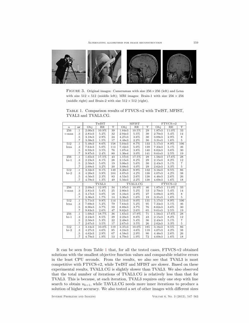
In the comparison, we tested two typical images (cameraman: 256×256 and lena:512× 512), two MRI brain images (br-1: 256× 256 and br-2: 512× 512). For eachimage, we tested four levels of sample ratios (defined by sr = m/n2): 10%, 30%,50% and 70%. The original images are displayed in Figure 3, while the comparisonresults are presented in Table 1, where the final objective function values (Obj), therelative errors (RE) of the recovered images to the true images, and the consumedCPU time in seconds (T) are given.
1Available at: http://www.lx.it.pt/~bioucas/TwIST/TwIST.htm2Available at: http://iew3.technion.ac.il/~becka/papers/tv_fista.zip3Available at: http://www.caam.rice.edu/~optimization/L1/TVAL3
Inverse Problems and Imaging Volume 6, No. 3 (2012), 547–563
Alternating algorithms for image reconstruction 559
Figure 3. Original images: Cameraman with size 256×256 (left) and Lena
with size 512 × 512 (middle left); MRI images: Brain-1 with size 256 × 256
(middle right) and Brain-2 with size 512 × 512 (right).
Table 1. Comparison results of FTVCS-v2 with TwIST, MFIST,TVAL3 and TVAL3 CG.
TwIST MFIST FTVCS-v2n sr Obj RE T Obj RE T Obj RE T
256 .1 2.00e3 10.9% 39 1.84e3 10.5% 29 1.87e3 11.0% 33c-man .3 2.81e3 5.2% 32 2.94e3 5.5% 30 2.70e3 5.4% 14
.5 3.18e3 2.9% 24 4.27e3 3.6% 30 3.09e3 2.9% 8
.7 3.38e3 1.5% 17 4.48e3 2.2% 30 3.31e3 1.6% 5512 .1 5.48e3 8.6% 158 5.04e3 8.7% 133 5.17e3 8.9% 106lena .3 7.64e3 5.0% 114 7.42e3 5.0% 139 7.33e3 5.1% 46
.5 8.92e3 3.5% 76 1.07e4 3.8% 140 8.62e3 3.6% 30
.7 9.87e3 2.4% 80 1.36e4 3.0% 141 9.61e3 2.5% 19256 .1 1.65e3 17.5% 43 1.57e3 17.5% 29 1.56e3 17.6% 28br-1 .3 2.23e3 8.1% 28 2.15e3 8.2% 29 2.15e3 8.2% 12
.5 2.50e3 5.0% 19 3.06e3 5.6% 30 2.43e3 5.1% 7
.7 2.68e3 3.2% 20 3.08e3 4.0% 29 2.62e3 3.3% 5512 .1 3.32e3 9.1% 149 3.20e3 9.9% 132 3.16e3 9.5% 86br-2 .3 4.20e3 3.9% 104 4.07e3 4.2% 138 4.07e3 4.2% 38
.5 4.56e3 2.3% 83 4.53e3 2.6% 138 4.46e3 2.6% 26
.7 4.78e3 1.3% 49 5.56e3 2.2% 138 4.69e3 1.6% 18
TVAL3 TVAL3 CG FTVCS-v2256 .1 2.09e3 12.9% 34 1.97e3 10.9% 46 1.87e3 11.0% 33
c-man .3 2.81e3 5.4% 25 2.80e3 5.2% 33 2.70e3 5.4% 14.5 3.17e3 3.0% 18 3.16e3 2.9% 27 3.09e3 2.9% 8.7 3.36e3 1.7% 14 3.36e3 1.6% 19 3.31e3 1.6% 5
512 .1 5.71e3 9.8% 114 5.51e3 9.0% 131 5.17e3 8.9% 106lena .3 7.69e3 5.2% 79 7.64e3 5.2% 95 7.33e3 5.1% 46
.5 8.90e3 3.7% 59 8.89e3 3.7% 76 8.62e3 3.6% 30
.7 9.83e3 2.6% 47 9.82e3 2.6% 65 9.61e3 2.5% 19256 .1 1.68e3 18.7% 36 1.65e3 17.9% 71 1.56e3 17.6% 28br-1 .3 2.24e3 8.5% 29 2.23e3 8.6% 43 2.15e3 8.2% 12
.5 2.50e3 5.3% 22 2.49e3 5.4% 36 2.43e3 5.1% 7
.7 2.67e3 3.5% 17 2.67e3 3.5% 26 2.62e3 3.3% 5512 .1 3.44e3 10.0% 119 3.37e3 10.0% 185 3.16e3 9.5% 86br-2 .3 4.27e3 4.6% 85 4.24e3 4.6% 118 4.07e3 4.2% 38
.5 4.62e3 2.9% 67 4.58e3 2.9% 90 4.46e3 2.6% 26
.7 4.79e3 1.9% 53 4.79e3 1.9% 72 4.69e3 1.6% 18
It can be seen from Table 1 that, for all the tested cases, FTVCS-v2 obtainedsolutions with the smallest objective function values and comparable relative errorsin the least CPU seconds. From the results, we also see that TVAL3 is mostcompetitive with FTVCS-v2, while TwIST and MFIST are slower. Based on theseexperimental results, TVAL3 CG is slightly slower than TVAL3. We also observedthat the total number of iterations of TVAL3 CG is relatively less than that forTVAL3. This is because, at each iteration, TVAL3 requires only one step with linesearch to obtain uk+1, while TAVL3 CG needs more inner iterations to produce asolution of higher accuracy. We also tested a set of other images with different sizes
Inverse Problems and Imaging Volume 6, No. 3 (2012), 547–563
560 Yunhai Xiao, Junfeng Yang and Xiaoming Yuan
and observed consistent results. Specifically, TVAL3 is the most competitive andruns slightly slower than FTVCS-v2, while TwIST and MFIST are slower. Theseresults and observations clearly demonstrated the efficiency and stability of theinexact ADM Algorithm 3.1.
5. Concluding Remarks. In this paper, based on the classical quadratic penaltymethod and the alternating minimization of the augmented Lagrangian functions,we proposed two fast alternating minimization algorithms for solving the total vari-ation image reconstruction model (3) with a generic linear operator. To overcomethe difficulty in solving a large linear system at each iteration, we adopted lin-earization and proximal techniques. The per-iteration cost of both algorithms isdominated by two matrix-vector multiplications and two FFTs. We also estab-lished finite convergence of certain variables and q-linear convergence rate for thequadratic penalty method. Our numerical comparisons with some state-of-the-artalgorithms also demonstrated the efficiency and stability of the inexact ADM ap-proach. With the encouraging numerical performance of the proposed algorithms,it is worthwhile to investigate other techniques such as the line-search strategies tofurther accelerate some splitting algorithms, which is an interesting topic of futureresearch.
Acknowledgments. We thank two anonymous referees for their constructive sug-gestions which improved the paper greatly.
Appendix A. Proof of Lemma 2.2.
Proof. Given (w1; v1) and (w2; v2), from the definition of q(w; v) and the nonex-pansiveness of S(·) (deduced from that of s(·) defined in (13)), it holds that
‖q(w1; v1)− q(w2; v2)‖2 ≤ ‖h(w1; v1)− h(w2; v2)‖2 + ‖p(w1; v1)− p(w2; v2)‖2
=∥∥R(w1 − w2; v1 − v2)
∥∥2,
where “≤” comes from the non-expansive of s(·) and R , (D; ηT )H−1(D; ηI)>. Itis easy to verify that
R>R
=
(DηI
)H−1(D>D + η2T 2)H−1
(DηI
)>=
(DηI
)H−1
(H − µ
β(2A>A− τ(A>A)2)
)H−1
(DηI
)>=
(DηI
)H−1
(DηI
)>− µ
β
(DηI
)H−1(2A>A− τ(A>A)2)H−1
(DηI
)>.
Recall that 0 < τ < 2/λmax(A>A), which ensures the positive semi-definiteness ofA>A− τ(A>A)2. Thus,
‖q(w1; v1)− q(w2; v2)‖2
≤(w1 − w2
v1 − v2
)>(DηI
)H−1
(DηI
)>(w1 − w2
v1 − v2
)≤∥∥∥∥ w1 − w2
v1 − v2
∥∥∥∥2
,(38)
Inverse Problems and Imaging Volume 6, No. 3 (2012), 547–563
Alternating algorithms for image reconstruction 561
where the second “≤” is from the definition of H. This implies that q(w; v) isnon-expansive.
Now we prove the second part of Lemma 2.2. We note that in the above proofthere are three “≤”. Thus, equality holds only when all the three inequalitiesbecome “=”. For simplicity, we let dw = w1 − w2 and dv = v1 − v2.
1. The first “≤” becomes “=” if and only if
S ◦ h(w1; v1)− S ◦ h(w2; v2) = h(w1; v1)− h(w2; v2) = DH−1
(DηI
)>(dwdv
).
2. The second “≤” becomes “=” if and only if(dwdv
)>(DηI
)H−1(2A>A− τ(A>A)2)H−1
(DηI
)>(dwdv
)= 0.
3. Let U be orthonormal and(DηI
)>H−1
(DηI
)= U>ΛU
be its eigenvalue decomposition. The third “≤” becomes “=” if and only if∑i
λi
(U
(dwdv
))2
i
=∑i
(U
(dwdv
))2
i
.
Since 0 ≤ λi ≤ 1, the above equality holds only when
λi
(U
(dwdv
))2
i
=
(U
(dwdv
))2
i
, ∀ i.
Therefore,
ΛU
(dwdv
)= U
(dwdv
),
and thus
(39)
(DηI
)H−1
(DηI
)>(dwdv
)=
(dwdv
).
From 1) and (39), we have
S ◦ h(w1; v1)− S ◦ h(w2; v2) = DH−1
(DηI
)>(dwdv
)= dw.(40)
From (39), the equality in 2) is equivalent to
dv>(2A>A− τ(A>A)2)dv = 0.
Let U>ΛU = A>A be the eigenvalue decomposition of A>A. The above equationis equivalent to
dv>U>(2Λ− τΛ2)Udv = 0 or∑i
(2λi − τλ2i )(Udv)2
i = 0.
Since 2λi − τλ2i ≥ 0, we have (2λi − τλ2
i )(Udv)2i = 0,∀ i. If λi 6= 0, then from the
choice of τ we have 2λi − τλ2i > 0, and thus (Udv)i = 0. Therefore, ΛUdv = 0 and
Inverse Problems and Imaging Volume 6, No. 3 (2012), 547–563
562 Yunhai Xiao, Junfeng Yang and Xiaoming Yuan
A>Adv = U>ΛUdv = 0. To sum up, we have
q(w1; v1)− q(w2; v2) =
(S ◦ h(w1; v1)− S ◦ h(w2; v2)
p(w1; v1)− p(w2; v2)
)=
(dwT · dv
)=
(dw
dv −A>Adv
)=
(w1 − w2
v1 − v2
),
where the first equality is from the definition of q(·; ·); the second one is from (40),the definition of p and (39); the third one is from the definition of T ; and the finalone is from A>dv = 0. This completes the proof.
REFERENCES
[1] R. Acar and C. R. Vogel, Analysis of total variation penalty methods, Inverse Prob., 10
(1994), 1217–1229.[2] M. V. Afonso, J. Bioucas-Dias and M. A. T. Figueiredo, Fastimage recovery using variable
splitting and constrained optimization, IEEE Trans. Image Process, 19 (2010), 2345–2356.[3] M. V. Afonso, J. Bioucas-Dias and M. A. T. Figueiredo, A fast algorithm for the constrained
formulation of compressive image reconstruction and other linear inverse problems, IEEE
Trans. Image Process, 20 (2011), 681–695.[4] J. Barzilai and J. M. Borwein, Two point step size gradient method , IMA J. Numer. Anal., 8
(1988), 141–148.
[5] A. Beck and M. Teboulle, Fastgradient-based algorithms for constrained total variation imagedenoising and deblurring problmes, IEEE Trans. Image Process, 18 (2009), 2419–2434.
[6] A. Beck and M. Teboulle, A fast iterative shrinkage-thresholding algorithm for linear inverse
problems, SIAM J. Imaging Sci., 2 (2009), 183–202.[7] J. Bioucas-Dias and M. Figueiredo, A new TwIST: Two-step iterative thresholding algorithm
for image restoration, IEEE Trans. Image Process, 16 (2007), 2992–3004.
[8] L. Bregman, The relaxation method of finding the common pointsof convex sets and its appli-cation to the solution of problems inconvex optimization, USSR Computational Mathematics
andMathematical Physics, 7 (1967), 200–217.
[9] E. Candes, J. Romberg and T. Tao, Robust uncertainty principles: Exact signal reconstructionfrom highly incomplete frequence information, IEEE Trans. Inform. Theory, 52 (2006), 489–
509.[10] A. Chambolle and P. L. Lions, Image recovery via total variation minimization and related
problems, Numer. Math., 76 (1997), 167–188.
[11] A. Chambolle and T. Pock, A first-order primal-dualalgorithm for convex problems withapplications to imaging, J. Math. Imaging Vis., 40 (2011), 120–145.
[12] T. F. Chan, S. Esedoglu, F. Park and A. Yip, “Recent Developments in Total Variation ImageRestoration,” TR05-01, CAM, UCLA, 2004.
[13] R. H. Chan, J. Yang and X. Yuan, Alternating direction method for image inpainting in
wavelet domain, SIAM J. Imaging Sci., 4 (2011), 807–826.
[14] P. L. Combettes and V. Wajs, Signal recoverty by proximal forward-backward splitting, Mul-tiscale Model. Simul., 4 (2005), 1168–1200.
[15] D. C. Dobson and F. Santosa, Recovery of blocky images from noisy and blurred data, SIAMJ. Appl. Math., 56 (1996), 1181–1198.
[16] B. Dong, J. Li and Z. Shen, X-ray CTimage reconstruction via wavelet frame based regular-
ization and Radon domain inpainting, J. Sci. Comput..[17] D. Donoho, Compressed sensing, IEEE Trans. Inform. Theory, 52 (2006), 1289–1306.
[18] R. G. Baraniuk, M. A. Davenport, M. F. Duarte, K. F. Kelly, J. N. Laska, T. Sun and D.
Takhar, Single Pixel Imaging via compressive sampling, IEEE Signal Processing Magazine,March 2008.
[19] E. Esser, “Applications of Lagrangian-Based Alternatingdirection Methods and Connections
to Split Bregman,” TR09-31, CAM, UCLA, Los Angeles, CA, 2009.[20] T. F. Chan, E. Esserand X. Zhang, A general framework for a class of first order primal-
dual algorithms for convex optimization in imaging science, SIAM J. Imaging Sci., 3 (2010),
1015–1046.[21] M. A. T. Figueiredo and R. Nowak, An EM algorithm for wavelet-basedimage restoration,
IEEE Trans. Image Process, 12 (2003), 906–916.
Inverse Problems and Imaging Volume 6, No. 3 (2012), 547–563
Alternating algorithms for image reconstruction 563
[22] D. Gabay and B. Mercier, A dual algorithm for the solution of nonlinear variational problemsvia finite-element approximations, Comput. Math. Appl., 2 (1976), 17–40.
[23] R. Glowinski and A. Marrocco, Sur lapproximation par elements finis dordre un, et la res-
olution par penalisation-dualite dune classe de problemes de Dirichlet nonlineaires, Rev.Francaise dAut. Inf. Rech. Oper., 2 (1975), 41–76.
[24] T. Goldstein and S. Osher, The split Bregman method forL1-Regularized Prolbems, SIAM J.Imaging Sci., 2 (2009), 323–343.
[25] E. T. Hale, W. Yin and Y. Zhang, A fixed-point continuation method for l1-regularized min-
imization with applications to compressed sensing, SIAM J. Optim, 19 (2008), 1107–1130.[26] B. He, D. Han, L. Z. Liao and H. Yang, A new inexact alternating directions method for
monotone variational inequalities, Math. Program, 92 (2002), 103–118.
[27] M. R. Hestenes, Multiplier and gradient methods, J. Optim.Theory Appl., 4 (1969), 303–320.[28] C. Li, “An Efficient Algorithm for Total Variation Regularization with Applications to the
Single Pixelcamera and Compressive Sensing,” Master thesis, Rice University, 2009.
[29] M. Defrise and C. De Mol, A note on wavelet-based inversion algorithms, Contemp. Math.,313 (2002), 85–96.
[30] M. J. D. Powell, A method for nonlinear constraints in minimization problems, in “Optimiza-
tion” (ed. R. Fletcher), Academic Press, New York, 1969, 283–298.[31] E. Fatemi, S. Osher and L. Rudin, Nonlinear total variation based noise removal algorithm,
Phys. D, 60 (1992), 259–268.[32] S. Setzer, “Split Bregman Algorithm, Douglas-Rachford Splittingand Frame Shrinkage,” Proc.
2nd International Conference on ScaleSpace Methods and Variational Methods in Computer
Vision, Lecture Notes in Computer Science, 2009.[33] F. Murtagh, M. Nguyen and J. L. Starck, Wavelets and curvelets forimage deconvolution: A
combined approach, Signal Processing, 83 (2003), 2279–2283.
[34] V. Arsenin and A. Tikhonov, “Solution of Ill-Posed Problems,” Winston, Washington, DC,1977.
[35] M. E. Oman and C. R. Vogel, Iterative methods for total variation denoising, SIAM J. Sci.
Comput., 17 (1996), 227–238.[36] M. E. Oman and C. R. Vogel, A fast, robust total variation based reconstruction of noisy,
blurred images, IEEE Trans. ImageProcess., 7 (1998), 813–824
[37] Y. Wang, J. Yang, W. Yin and Y. Zhang, A new alternating minimization algorithm for totalvariation image reconstruction, SIAM J. Imaging Sci., 1 (2008), 248–272.
[38] Y. Wang, J. Yang, W. Yin and Y. Zhang, A fast algorithm for edge-preserving variational
multichannel image restoration, SIAM J. Imaging Sci., 2 (2009), 569–592.[39] J. Yang, and Y. Zhang, Alternating direction algorithms forL1-problems in compressive sens-
ing, SIAM J. Sci. Comput., 33 (2011), 250–278.[40] J. Yang, W. Yin and Y. Zhang, An efficient TVL1 algorithm for deblurring multichannel
images corrupted by impulsive noise, SIAM J. Sci. Comput., 31 (2009), 2842–2865.[41] Y. Zhang, “Theory of Compressive Sensing Via`1-Minimization: A Non-RIP Analysis and
Extensions,” TR08-11, CAAM, Rice University, 2008.
Received February 2011; revised January 2012.
E-mail address: [email protected] address: [email protected] address: [email protected]
Inverse Problems and Imaging Volume 6, No. 3 (2012), 547–563