Alternative Functional Forms and Errors of Pseudo Data Estimation

Alternative Functional Forms and Errors of Pseudo Data EstimationAuthor(s): G. S. Maddala and R. Blaine RobertsSource: The Review of Economics and Statistics, Vol. 62, No. 2 (May, 1980), pp. 323-327Published by: The MIT PressStable URL: http://www.jstor.org/stable/1924768 .

Accessed: 28/06/2014 09:50

Your use of the JSTOR archive indicates your acceptance of the Terms & Conditions of Use, available at .http://www.jstor.org/page/info/about/policies/terms.jsp

.JSTOR is a not-for-profit service that helps scholars, researchers, and students discover, use, and build upon a wide range ofcontent in a trusted digital archive. We use information technology and tools to increase productivity and facilitate new formsof scholarship. For more information about JSTOR, please contact [email protected].

.

The MIT Press is collaborating with JSTOR to digitize, preserve and extend access to The Review ofEconomics and Statistics.

http://www.jstor.org

This content downloaded from 193.105.245.179 on Sat, 28 Jun 2014 09:50:59 AMAll use subject to JSTOR Terms and Conditions

http://www.jstor.org/action/showPublisher?publisherCode=mitpress

http://www.jstor.org/stable/1924768?origin=JSTOR-pdf

http://www.jstor.org/page/info/about/policies/terms.jsp


NOTES 323

these restrictions. I subsequently imposed and tested the smoothness conditions (equations (7) to (10)) and, on the basis of the F-test, accepted these restrictions as well.7 Thus, I conclude that a four segment smooth quadratic spline adequately captures the seasonal pattern in this relationship. The final form of the estimated equation, using the form of equation (13), is

y(t) = -.86 - .20*S3 - .065*S6 - .091*S9

(2.8) (3.0) (1.0) (1.5) + .81 *x(t)

(13.6)

R2= .6420 (14)

where the terms in parentheses are t-statistics.8 The shape of the seasonal pattern can be found from the first four terms. The exact plot of this seasonal pattern is, in fact, that given in diagram 1.

REFERENCE

Suits, Daniel B., Andrew Mason and Louis Chan, "Spline Functions Fitted by Standard Regression Methods," this REVIEW 60 (Feb. 1978), 132-139.

7 The F-statistic for the first test is F(4,107) = 0.50 while for the second test it is F(4,11 1) = 0.81. Both of these values are well below the critical-F at conventional levels of sig- nificance.

8 Further experimentation showed that one additional pa- rameter could be eliminated by, for example, disposing of the last join point (setting d2 = 0.). However, since the purpose here was simply to show that fewer than 12 parameters are required, the equation has been left in the present form.

ALTERNATIVE FUNCTIONAL FORMS AND ERRORS OF PSEUDO DATA ESTIMATION

G. S. Maddala and R. Blaine Roberts*

I. Introduction

Griffin (1977a, 1978) has recently suggested the method of pseudo data analysis as a useful approach to analyze process models. There are many advantages claimed for this procedure. Griffin (1977a, p. 389) says:

Unlike most time series data, pseudo data provide detailed data on specific input and output quantities. Since the data are not constrained by historical variation, multicollinearity among input and output prices is effec- tively eliminated.

According to Griffin (p. 389), pseudo data analysis is

. . . aimed at distilling the complex process analysis representation into a single equation, statistical approximation to the joint production technology. This alternative provides both a direct source of price and substitution elasticities and a convenient form for micro- econometric modeling exercises.

The purpose of this paper is to present some results from a pseudo data analysis of a small hypothetical process model that casts doubt about the usefulness of the approach. In section II, we discuss: (1) the statistical properties of the errors; (2) the question of the appropriate norm for approximation errors; (3) the alternative functional forms; and (4) the issue of single versus multiple equation methods of estimation. In section III, we present an illustrative analysis of a small process model and the resulting elasticities. A summary and conclusions are contained in section IV.

II. Aspects of Fitting Equations to Pseudo Data

Griffin (1977a, p. 393) argues that there are two sources of error: an approximation error and an error that arises from the fact that the technical coefficients are only estimates of the true coefficients. However, the errors in the technical coefficients of the process model are just that and are not a stochastic influence on the pseudo data.

The errors in pseudo data analysis arise entirely from not having the correct functional form. Though this is one of the components in the error term often mentioned in econometrics textbooks, these textbooks also argue that this is only one of many sources and there are other sources like errors in measurement in the dependent variable, omitted variables, etc. It is the multiplicity of errors that enables one to invoke the central limit theorem so as to justify the assumption of normality for the residuals in econometric equations.

Received for publication June 28, 1978. Revision accepted for publication May 10, 1979.

* University of Florida and University of South Carolina, respectively.

This research was supported under contract number RP 867-2 from the Electric Power Research Institute to A. L. Fletcher & Associates. The opinions expressed are those of the authors and not of E.P.R.I. We would like to thank L. J. Lau, J. M. Griffin, and a referee for helpful comments. Need- less to say, they do not necessarily agree with the conclusions of our paper.



324 THE REVIEW OF ECONOMICS AND STATISTICS

In the case of the pseudo data problem there is just one source of error. This is purely an approximation error. It is true that these approximation errors are systematically related to the price vector chosen in the linear programming problem. But they will also be dependent on the functional form chosen for the approximation. The correlation between the error term and the prices is of consequence only if we want to attribute the usual statistical properties to the estimates. But since this is not meaningful here anyway, we need not worry at all about this correlation. What is of consequence is the magnitude of the approximation error and the sensitivity of the parameters of the approximating function.

In all the methods that Griffin used and that we use later, the closeness of the approximation of the continuous function to the data points is measured by the sum of squares of the residuals. This is the "least squares norm." One can think of other norms for minimization purposes: sum of absolute errors or the sum of some power of these errors. These alternative norms involve more computational burdens than the least squares norm and we feel that not much is to be gained by going to these complicated methods. The main purpose in getting the approximating continuous function is to minimize the computational burdens in repeatedly solving the original process model. The question of these alternative norms increases the computational burden at this point and diverts attention to an issue of secondary importance from issues that are more fundamental to the analysis of pseudo data.

There are a variety of functional forms that can be used as approximating, continuous functions for the pseudo data. In our work, we tried Cobb-Douglas, constant elasticity of substitution (CES), and the translog. Traditionally, in the estimation of the translog cost functions, it has been found that one got poor results if the cost function was estimated by single equation methods. This is due to the multicollinearity problem. Hence, it has become customary to use the share equations as well and estimate the whole set of equations by system methods. Because with pseudo data (at least the way Griffin generated the data) we do not have the multicollinearity problem, multiple equation methods are not necessary. Another case where multiple equations have been suggested is where ordi- nary least squares (OLS) estimation of the production function gives inconsistent estimates (see Nerlove (1965)) and one needs to estimate the structural model. Again, this sort of protlem does not arise in the estimation of cost functions or price possibility frontiers with pseudo data. The explanatory variables are all exogenous.

III. An Illustrative Analysis of a Process Model

Initially, we were going to use a real world process model. However, these models are much too unwieldy

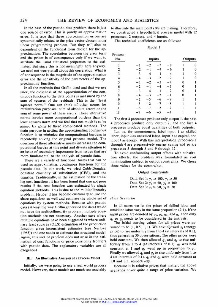
to illustrate the main points we are making. Therefore, we constructed a hypothetical process model with 12 processes, 2 outputs, and 4 inputs.

The technical coefficients are as follows:

Model 1

Process No. Inputs Outputs

1 -1 -2 -3 -8 1 0 2 -2 -1 -4 -6 1 0 3 -3 -4 -1 -4 1 0 4 -4 -3 -2 -2 1 0 5 -1 -2 -3 -4 0 1 6 -2 -1 -4 -3 0 1 7 -3 -4 -1 -2 0 1 8 -4 -3 -2 -1 0 1 9 -2 -5 -6 -9 1 1

10 -5 -2 -7 -8 1 1 11 -6 -7 -2 -7 1 1 12 -7 -6 -5 -4 1 1

- The first 4 processes produce only output 1, the next 4 processes produce only output 2, and the last 4 processes produce equal quantities of both outputs.

Let us, for concreteness, label input 1 as skilled labor, input 2 as unskilled labor, input 3 as capital, and input 4 as energy. With this interpretation, processes 1 through 4 are progressively energy saving and so are processes 5 through 8 and 9 through 12.

To avoid confounding output effects with substitution effects, the problem was formulated as cost minimization subject to output constraints. We chose three values for the constraints.

Output Constraints

Data Set 1: Yi , 100, Y2 ? 50 Data Set 2: Yi ? 50, Y2 ? 100 Data Set 3: Yi , 50, Y2 ? 50

Price Scenarios

In all cases we let the prices of skilled labor and unskilled labor vary in the same proportion (2: 1). If the input prices are denoted by q1, q2, q3, and q4, then only

q, or q2 needs to be considered in the analysis. The initial starting values for all prices were as-

sumed to be (1, 0.5, 1, 1). We next aJ,owed q4 (energy price) to rise uniformly from I to 4 (at intervals of 0.1), thus generating 30 observations. The other prices were held constant. We then allowed q1 and q4 to rise uniformly from 1 to 4 (at intervals of 0.1). q3 was held constant at 1 and q2 went up in proportion to q1. Finally we allowed q3 and q4 to rise uniformly from 1 to 4 (at intervals of 0.1). q1 and q2 were held constant at 1.0 and 0.5, respectively.

Because it is relative prices that matter, the above scenarios cover quite a range of price variation. We



NOTES 325

have thus 91 observations in all. Instead of letting the prices quadruple, we also considered the case where prices triple, giving 61 observations, but since the results and conclusions are the same as for the previous case, we will not report the results here.

What we found was that all the functional forms gave very good fits. The R2s were very high. For the Cobb-Douglas they were 0.9865, 0.9867, 0.9922. For the CES they were 0.9998, 0.9913, 0.9994. For the translog they were 0.99993, 0.99983, 0.99991. Nor was multicollinearity any problem. For instance, the t-ratios for the first set of data for the translog ranged from 18 to 232. All this would lead one to believe (as Griffin often argued) that one is getting an excellent approximation to the technology of the process model. But the elasticities, presented in table 1, show that this is indeed not the case.

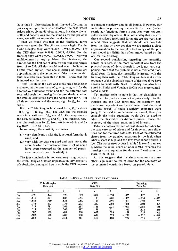
Table 1 contains the own and cross price elasticities evaluated at the base case of q1 = q3 = q4 = 1 for the alternative functional forms and for the different data sets. Although the translog fits the pseudo data better, the implied elasticities have the wrong sign for E1l for all three data sets and the wrong sign for E44 for data set 3.

For the Cobb-Douglas functional form, E1l is about --0.5, E33 -0.8, E44 -0.7. The CES and the translog result in an estimate of E1l near 0.0. Also very low are the CES estimates for E33 and E44. The translog, however, has estimates for E33 from -0.44 to -0.84 and for E44 from -0.32 to +0.25.

In summary, the elasticity estimates:

(1) vary significantly with the functional form that is used; and

(2) vary with the data set used and vary more, the more flexible the functional form is. (This could have been expected as the number of parameters increases with flexibility.)

The first conclusion is not very surprising because the Cobb-Douglas function imposes a unitary elasticity of substitution among all inputs while the CES imposes

a constant elasticity among all inputs. However, our motivation in presenting the results for these (rather restricted) functional forms is that they were not considered earlier by others. It is noteworthy that even for these restricted functional forms the R2s are very high indeed. This suggests that we should not conclude from the high R2s we get that we are getting a close approximation to the complex technology of the process model (as Griffin has often argued based on the R2s for the translog).

Our second conclusion, regarding the instability across data sets, is the more important one from the practical point of view, though it too is not very surprising. Note that the problem is not a restricted functional form. In fact, this instability is greater with the translog than with the Cobb-Douglas. Nor is it a consequence of the simplistic nature of the model we have chosen to work with. Such instability has also been noted by Smith and Vaughan (1978) with more complicated models.

Yet another point to note is that the elasticities in table 1 are for the base case set of prices only. For the translog and the CES functions, the elasticity estimates are dependent on the estimated cost shares at different prices. If these elasticity estimates were going to be used in an econometric model, then presumably the share equations would also be used to adjust the elasticities for different prices. Hence, the accuracy of the share equation is of interest.

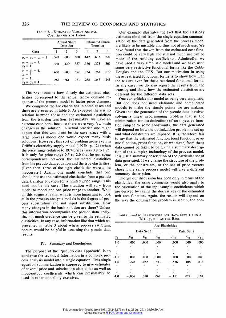
Table 2 contains the actual cost shares for labor for the base case set of prices and for three extreme situa- tions and for the three data sets. Each of the estimated shares from the translog equations is too high when labor's share is high and too low when labor's share is low. The worst error occurs in table 2 in row 3, data set 2, where the actual share of labor is 50%, whereas the translog share equation for data set 2 estimates the share to be 76.1%.

All this suggests that the share equations are another, significant source of error for the accuracy of the estimated elasticities based on pseudo data.

TABLE 1.-OWN AND CROSS PRICE ELASTICITIES

Cobb-Douglas CES Translog Data Set Data Set Data Set

1 2 3 1 2 3 1 2 3

-.498 - .474 - .520 -.029 - .057 - .098 .053 .076 .061 -.816 -.807 -.846 -.055 -.113 -.201 -.439 -.839 -.622 -.686 -.719 -.634 -.056 -.118 -.191 -.003 -.323 .253

.184 .193 .154 .213 .217 .180 .038 .004 .095

.314 .281 .366 .197 .181 .221 - .091 -.080 -.156

.314 .281 .366 .197 .181 .221 .310 .832 .259

.502 .526 .480 .590 .602 .599 .128 .016 .363

.502 .526 .480 .590 .609 .599 - .271 - .232 - .448

.184 .193 .154 .213 .217 .180 .274 .555 .195



326 THE REVIEW OF ECONOMICS AND STATISTICS

TABLE 2.-ESTIMATED VERSUS ACTUAL

COST SHARES FOR LABOR

Actual Share Estimated Share Data Set Translog

Case 1 2 3 1 2 3

q, = q3 = q4= 1 .593 .608 .600 .612 .635 .621

ql = q3= 1, .388 .429 .387 .360 .373 .301

q4 = 4

q, = q4 = 4, .600 .500 .552 .734 .761 .679 q3 = I

_ 1

q1= 1, .267 .261 .273 .238 .247 .243 q3 = q4 = 4

The next issue is how closely the estimated elasticities correspond to the actual factor demand re- sponse of the process model to factor price changes.

We computed the arc elasticities in some cases and these are presented in table 3. As expected there is no relation between these and the estimated elasticities from the translog function. Presumably, we have an extreme case here, because there were very few basis changes in the solution. In actual practice one might expect that this would not be the case, since with a large process model one would expect many basis solutions. However, this sort of problem arose even in Griffin's electricity supply model (1977b, p. 124) when the price range (relative to 1974 prices) was 0.8 to 1.25. It is only for price range 0.5 to 2.0 that he got some correspondence between the estimated elasticities from his pseudo data equation and the true elasticities. (Even then, three of the eight elasticities were quite inaccurate.) Again, one might conclude that one should not use the estimated elasticities from a pseudo data translog equation for a limited price range. This need not be the case. The situation will vary from model to model and one price range to another. What all this suggests is that what is more important to look at in the process-analysis models is the degree of process substitution and not input substitution. How many changes in the basis solution are there? Unless this information accompanies the pseudo data analysis, not Mbuch credence can be given to the estimated elasticities. In any case, information like that which we presented in table 3 about where process switching occurs would be helpful in assessing the pseudo data results.

IV. Summary and Conclusions

The purpose of the "pseudo data approach" is to condense the technical information in a complex process analysis model into a single equation. This single equation summarization is supposed to give estimates of several price and substitution elasticities as well as input-output coefficients which can presumably be used in other modelling exercises.

Our example illustrates the fact that the elasticity estimates obtained from the single equation summarization of the data generated from the process model are likely to be unstable and thus not of much use. We have found that the R2s from the estimated cost function could be very high and still not much use can be made of the resulting coefficients. Admittedly, we have used a very simplistic model and we have used some very restrictive functional forms like the Cobb- Douglas and the CES. But our motivation in using these restricted functional forms is to show how high the R2s are even for these restricted functional forms. In any case, we do also report the results from the translog and show how the estimated elasticities are different for the different data sets.

One can criticize our model as being very simplistic. But one does not need elaborate and complicated models to make the simple points we are making. Given that the generation of the pseudo data involves solving a linear programming problem that is the minimization (or maximization) of an objective function subject to some constraints, the data generated will depend on how the optimization problem is set up and what constraints are imposed. It is, therefore, fair to say that the estimated function (cost function, reve- nue function, profit function, or whatever) from these data cannot be taken to be giving a summary description of the complex technology of the process model. It is just a summary description of the particular set of data generated. If we change the structure of the problem, or the constraints, or the set of price vectors chosen, the same process model will give a different summary description.

Though our discussion has been only in terms of the elasticities, the same comments would also apply to the calculation of the input-output coefficients which are derived by taking the derivatives of the estimated unit cost function. Again, the results will depend on the way the optimization problem is set up, the con-

TABLE 3.-ARC ELASTICITIES FOR DATA SETS 1 AND 2 WITH q4 = t AS THE BASE

Arc Elasticities

Data Set 1 Data Set 2

q4 E44 E14 E34 E44 E14 E34

1.0 .000 .000 .000 .000 .000 .000

1.5 .000 .000 .000 .000 .000 .000

1.6 -.278 .052 .333 -.556 .108 .833

4.0 -.006 .010 .067 -.111 .022 .167



NOTES 327

straints that are imposed, the price vectors chosen to generate the pseudo data, and the functional form used for the cost function approximation. It is also fair to say that if input-output coefficients are the ones of interest, since these are obtained for each of the points used in the pseudo data generation, it may be better to seek some approximating functions for these directly rather than seek an approximating function for the cost function and then derive the input-output coefficients.

All these comments do not imply that the "pseudo data" approach should be given up. It is, however, important to sort out the aims of the analysis. There are some problems (like studying the effects of changes in environmental regulations) where one cannot get any answers from time series data and one has to use the process analysis models that have detailed specification of technology and the constraints. But for this the appropriate thing is to do a simulation analysis of the process model itself and not seek a single equation approximation of the complex technology. What

distin,guishes Griffin's approach from the garden variety simulation analyses of process models is this "dis- tillation" in a single equation.

REFERENCES

Griffin, James M., "The Econometrics of Joint Production: Another Approach," this REVIEW 59 (Nov. 1977a), 389-397.

"Long-run Production Modelling With Pseudo-data: Electric Power Generation," The Bell Journal of Eco- nomics 8 (Spring 1977b), 112-127. , "Joint Production Technology: The Case of Pet- rochemicals," Econometrica 46 (1978), 379-396.

Nerlove, Marc, Estimation and Identification of Cobb- Douglas Production Functions (Amsterdam: North- Holland Publishing Company, 1965).

Smith, V. Kerry, and W. J. Vaughan, "The Revival of En- gineering Approaches to Production Analysis: Estima- tion With Pseudo-data," Discussion paper D-38, Re- sources for the Future, July 1978.

ALTERNATIVE FUNCTIONAL FORMS AND ERRORS OF PSEUDO DATA ESTIMATION: A REPLY

James M. Griffin*

The skepticism of Professors Maddala and Roberts (1980) regarding the value of the pseudo data approach, outlined in Griffin (1977), rests on the accuracy with which the production surface implied by a process model can be approximated by a statistical cost or profit function estimated from points drawn from that surface. Using a hypothetical process model, they demonstrate that not only do the estimated elasticities differ (i) between functional forms and (ii) data sets, but (iii) the estimates also differ substantially from the actual arc elasticities. In addition, they argue (iv) that errors in the predicted cost shares further exacerbate the errors in the elasticity calculation. A close examination of their model and methodology reveals that these conclusions follow from a very simplistic process model and a specious criterion for elasticity comparisons. Each point is considered in order.

With respect to (i), Maddala and Roberts show in their table 1 thatfor the same data set, the elasticity estimates obtained by a Cobb-Douglas, constant elasticity of substitution (CES), and translog cost function

are quite different. They note that even though the translog yields the highest R2, it implies perverse own price elasticities for 2 of the 3 inputs1 when evaluated at the "base case" set of prices. What is not apparent is that their "base case" price vector is in fact a sample extremum from which prices are varied four- fold.2 Is it surprising that the Cobb-Douglas, CES, and translog functions yield different extreme point elasticities since they differ substantially in their restrictions on the elasticity of substitution? One could expect to obtain this result with any data set-time series, cross sections, or pseudo data. Furthermore, is it surprising that perverse elasticities are observed at this extreme "base case," given that the translog pur- ports only to offer a local, not a global approximation? The relevant question is not whether perverse elasticities occur at such sample extremes, but rather do they occur frequently for the sample means and the most likely forecast range?

With respect to (ii), Maddala and Roberts find in

Received for publication July 30, 1979. Accepted for publication September 4, 1979.

* University of Houston.

I They combine labor types 1 and 2, treating it as an aggre- gate.

2 In their notation, q, = q3 = q4 =1 as the "base case" prices. Thirty observations were obtained by holding q1 = q3 = 1 and varying q4 from 1 to 4 by increments of 0.1. Next, holding q3 = 1, q, and q4 were varied from I to 4. Finally, q3

and q4 were varied from 1 to 4 while holding q, = 1.



Documents

Alternative Functional Forms and Errors of Pseudo Data Estimation