NPV ' jn

t'1

Ct

(1 % k)t& C0

' PVCF & Initial Investment

ALTERNATIVE INVESTMENT RULES

2 Net Present Value (NPV)

Decision Rule: Accept if NPV > 0

Economic Meaning of NPV?

2 Example & Consider investments A and B (k=10%)

Year A B

0 ($1,000) ($1,000)

1 500 100

2 400 200

3 300 300

4 100 400

5 10 500

6 10 600

NPVA = $500(PVIF10,1) + 400(PVIF10,2) + 300(PVIF10,3) + 100(PVIF10,4) + 10(PVIF10,5) + 10(PVIF10,6) - $1000

= $1091 - $1000

= $91

NPVB = $403

Decision:

NPV > 0 Accept

NPV > 0 Accept

AROI ' Accounting Profit

Accounting Investment

OTHER CONTENDERS

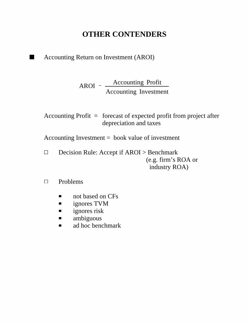
2 Accounting Return on Investment (AROI)

Accounting Profit = forecast of expected profit from project afterdepreciation and taxes

Accounting Investment = book value of investment

4 Decision Rule: Accept if AROI > Benchmark(e.g. firm’s ROA or industry ROA)

4 Problems

3 not based on CFs3 ignores TVM3 ignores risk3 ambiguous3 ad hoc benchmark

PB ' (T & 1) %

C0 & jT&1

t'1

Ct

CT

2 Payback Method

Number of years until cumulative forecasted CFs equal initialinvestment

T = number of years until investment is completely recovered bycumulative CFs.

4 Decision Rule: Accept if PB < Benchmark

PBA = (3 - 1) + = 2 1/3 years$ 1 0 0 0 & $900

$300

PBB = (4 - 1 ) + = 4 years$1000&$600

$400

4 Advantages

3 easy, inexpensive, intuitive3 some indication of risk and liquidity

4 Disadvantages

3 ad hoc PB benchmark3 ignores risk of CFs

3 Ignores CFs beyond PB period

Example: C E0 ' C D

0 ' $10,000

Year CFC CFD

1 $5000 $10,000

2 5000 0

3 20,000 1,000

PBC = 2 yrs.

PBD = 1 yr.

3 Ignores TVM (equal weight gives to each CF)

Example: C E0 ' C F

0 ' $1,001,000

Year CFC CFD

1 ± 0 $1,000,000

2 1,000,000 0

3 1,000 1,000

4 500,000 500,000

PBE = PBF = 3 yrs.

* Discounted Payback

3 discounts each CF at cost of capital3 finds "how many years CFs must be received from the

investment for it to make sense from an NPV standpoint"3 overcomes "equal weighting" and risk problems to some

extent3 still ignores CFs beyond PB3 benchmark is still ad hoc

r ' rate of return '

Payoff

Cost& 1 '

C1

C0

& 1 (1)

C1

(1 % r)& C0 ' 0 (2)

NPV '

C1

(1 % k)& C0 (3)

2 Internal Rate of Return (IRR)

Measures rate of return that an investment earns

4 IRR defined as "rate of return that makes PVCFs equal toinitial costs"

4 Single Period

Rearranging (1) gives

Remember

So IRR is the return level, r, that would make NPV = 0.

Note that if , then NPV 0.r>

<k

>

<

Decision rule: Accept if r > k.

C 1

(1 % r)%

C2

(1 % r)2% ä %

Cn

(1 % r)n' C0

jn

t'1

Ct

(1 % r)t& C0 ' 0 (NPV(r) ' 0)

4 For multi-year investments r, is defined as

or

4 Finding IRRs

3 Annuities

Investment cost = $10,000CFs at end of years 1-10 = $1,627.45

PMT(PVIFAr,10) = $10,000C(PVIFAr,10) = C0

$1,627.45(PVIFAr,10) = $10,000

PVIFAr,10 = 6.1446 (table value)

r = 10%

Accept if 10% > k

4 Uneven streams of CFs

Trial and error

3 Find PVCF at (start at 10%)$r3 If PVCF > I then 8 $r3 If PVCF < I then 9 $r3 Repeat until PVCF = I at which $r ' r

Example: Investment A

PVCFA = 500(PVIF10,1) + 400(PVIF10,2) + 300(PVIF10,3)+ 100(PVIF10,4) + 10(PVIF10,5) + 10(PVIF10,6)

= $1091

(PVCFA(10%) = $1091) = (Cost = $1000)

Try = 15%$r

(PVCFA(15%) = $1000) = (Cost = $1000)

rA = 15% (IRRA)

(IRRB = 20%)

Example: PVCFB(20%) = $1,000

rb =20% (IRRB)

4 Profitability Index (PI)

Benefit

Cost Ratio

PI = j

n

t'1

Ct

(1 % k)t

C0

'

PVCF

I

Decision Rule: Accept if PI > I

PIA = = 1.091 > 1 Accept$1091

$1000

PIB = = 1.403 > 1 Accept$1403

$1000

CRITERIA FOR CHOOSING INVESTMENTDECISION RULE

2 Decision Process

4 Identify new strategies and opportunities4 Estimate expected cash flows4 Apply decision rule to choose strategy

2 Decision Rule Should Maximize Value

4 All CFs should be considered4 CFs should be weighted by opportunity cost of investment

funds4 rule should select value maximizing strategy from a set of

mutually exclusive investments 4 rule should allow projects to be considered independently

COMPARISON BETWEEN NPV, IRR, AND PI

2 Remember the decision rules

Investment RuleDecision

NPV IRR PI

NPV = 0 r = k PI = 1 ?

NPV > 0 r > k PI > I Accept

NPV < 0 r < k PI < I Reject

Each rule appears to select the same strategy. However, we’ll seethat IRR and PI have some weaknesses, the biggest of which is thatthey don’t always maximize value.

2 Definitions

4 Independent Project % Projects CFs are independent ofother project’s CFs

4 Mutually Exclusive Projects % Project’s CFs are related toother project’s CFs

2 Investment Type Problems

4 Consider Investment A: Invest $100 today and receive $130next year (r=30%)

Alternative: Invest $100 at k

Suppose k = 25% : $100 (1 + .25) = $125k = 35% : $100 (1 + .35) = $135

So IRR decision rule (r > k) makes sense

In terms of NPV:

NPVA(k=25%) = - $100 = $4.00 > 0 (Accept A)$130

(1 % .25)

NPVA(k=35%) = - $100 = -$3.70 < 0 (Reject A)$130

(1 % .35)

Graphically

IRR DecisionRule: Accept if r > k or whenever .3 > k

2 Financing Type Problems

4 Now consider Project B: Receive $100 and payout $130 nextyear (r=30%)

Alternatives:

Suppose k = 25% : $100 (1 + .25) = $125 payout

k = 35% : $100 (1 + .35) = $135 payout

In terms of NPV:

NPVB(25%) = + 100 = -$4.00 (Reject B)&130

(1 % .25)

NPVB(35%) = + 100 = $3.70 (Accept B)&130

(1 % .35)Decision rule is "opposite" for financing type problems

IRR Decision Rule: Accept if k > r

Project is actually a substitute for borrowing. If you can borrow elsewherefor less, then reject project. Haven’t really addressed risk issue

Result:

Investment-type projects: Accept if r > k

Financing-type projects: Accept if r < k

Decision rule is reversed but not a problem if understood.

2 Multiple IRRs

Oil-well pump problem

An oil company is trying to decide whether or not to install a high-speed pump on a well that is already in operation. Cost of capital is10%.

Year CF 0 - 1600 1 +10,000 2 - 10,000

NPV = - 1600 = -773.5510,000

(1 % .10)%

&10,000

(1 % .10)2

To find IRR

1 0 , 0 0 0

( 1 % r)%

&10,000

(1 % r)2& 1600 ' 0

Note both r = 25% and r = 400% satisfy IRR definition

10,000

(1 % .25)%

&10,000

(1 % .25)' &1600 ' 0

10,000

(1 % 4)%

&10,000

(1 % 4)' &1600 ' 0

Multiple IRRs are the result of sign changes in the CF stream.

Let’s look again at the definition of IRR for this problem

10,000

(1 % r)%

&10,000

(1 % r)2& 1600 ' 0

Multiply both sides by (1 + r) 2

10,000 (1 % r) & 10,000 & 1600(1 % r)2' 0

or

10,000 - 10,000 (1 + r) + 1600 (1 + r) 2 = 0

The IRR is the solution to the quadratic equation

ax2 + bx + c = 0

where a = 1600, b = -10,000, c = 10,000, and x = (1 + r)

The solution is given by the quadratic formula

x '

&b ± b 2& 4ac

2a

(1 +r) = 10,000 ±

10,0002& 4(1600)(10,000)

2(1600)

(1 + r) = 10,000 ± 6000

3200

r = 25% or 400%

IRR decision rule no longer maximizes NPV.

Decarte's rule of signs implies m sign changes yields m possibleIRRs.

Only safe to use IRR method with 1 sign change.

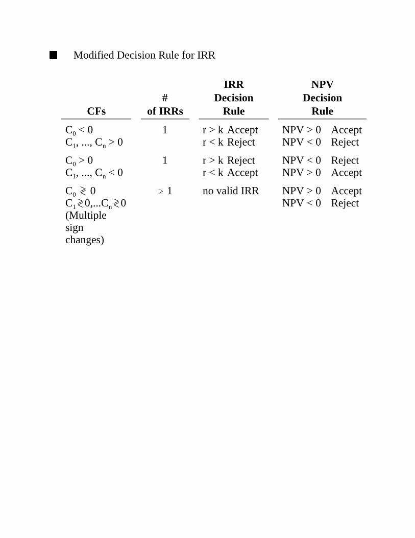
2 Modified Decision Rule for IRR

CFs#

of IRRs

IRRDecision

Rule

NPVDecision

Rule

C0 < 0C1, ..., Cn > 0

1 r > k Acceptr < k Reject

NPV > 0 AcceptNPV < 0 Reject

C0 > 0C1, ..., Cn < 0

1 r > k Rejectr < k Accept

NPV < 0 RejectNPV > 0 Accept

C0 0><C1 0,...Cn 0>< ><(Multiplesignchanges)

$ 1 no valid IRR NPV > 0 AcceptNPV < 0 Reject

2 Reinvestment Rate Assumption

Both NPV and IRR make explicit assumptions about how cash flowsare reinvested.

Consider the Net Future Value (NFV) of an investment defined asthe amount of cash available at period n in excess of the cash youcould have received investing elsewhere.

NFV = [CF1 (1 + k)n-1 + C2 (1 + k)n-2 + . . . . Cn] - C0 (1 + k)n

This NFV is the net "profit" or "value" of the investment at time nassuming the CFs are invested at k each period.

Again, assuming we can earn k elsewhere,

NPV '

NFV

(1 % k)n'

C1 (1 % k)n&1

(1 % k)n%

C2 (1 % k)n&2

(1 % k)n% ä

Cn

(1 % k)n&

C0 (1 % k)n

(1 % k)n

'

C1

(1 % k)% ä

Cn

(1 % k)n& C0

NPV assumes CFs and NPV can be invested at k.

2 Similarly, the IRR can be thought of in terms of NFV:

NFV(r) = [C1 (1 + r)n-1 + ... Cn] - C0 (1 + r)n = 0

or

N P V '

NFV

(1 % r)n'

C1 (1 % r)n&1

(1 % r)n% ä

cn

(1 % r)n&

C0 (1 % r)n

(1 % r)n' 0

'

C1

(1 % r)% ä

Cn

(1 % r)n& C0 ' 0

So IRR assumes CFs are reinvested at r.

2 Assuming reinvestment at k is more realistic

k is a market determined return for a given risk level

IRR assumes each project with a different r can earn a differentreturn (r) on reinvested CFs, even though the projects may have thesame risk level.

IRR doesn’t discount CFs at opp. cost of capital.

jn

t'1

Ct (1 % k)n&t& C0 (1 % r)n

' 0

r 'j

n

t'1

Ct (1 % k)n&t

C0

1

n

& 1

2 Modified IRR & we can modify IRR rule by improvingassumptions about reinvestment.

Assuming CFs are reinvested at k gives a future value of the CFs atn of:

FVn = [C1 (1+ k)n-1 + . . . . . . Cn]

Modified IRR is the return on C 0 that makes

FVn = C0 (1 + r)n

Eliminates problem with multiple IRRs.

Consider again the oil-well pump example

r '10,000 (1 % .10) % (&10,000)

1600

1

2& 1 ' &.2094

Reject Y now consistent with NPV

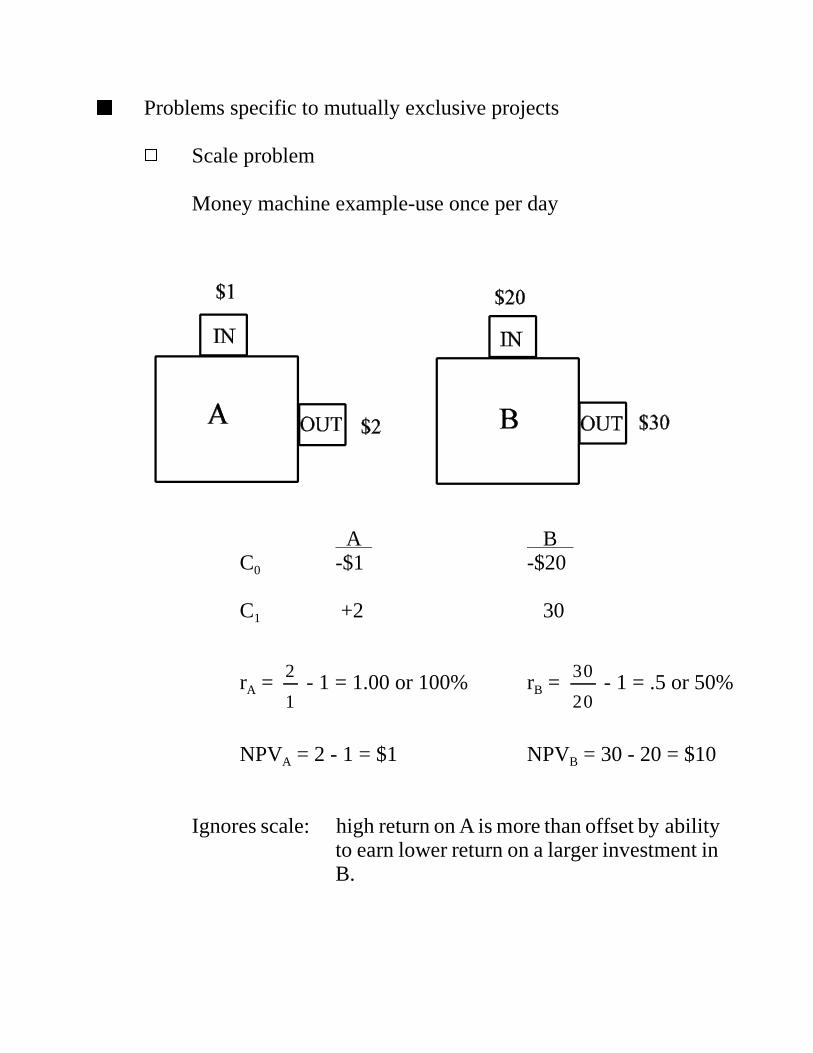
2 Problems specific to mutually exclusive projects

4 Scale problem

Money machine example-use once per day

A B C0 -$1 -$20

C1 +2 30

rA = - 1 = 1.00 or 100% rB = - 1 = .5 or 50%2

1

30

20

NPVA = 2 - 1 = $1 NPVB = 30 - 20 = $10

Ignores scale: high return on A is more than offset by abilityto earn lower return on a larger investment inB.

Example 2 & C + D are mutually exclusive

Time C DIncremental

CF(D - C)

0 -1000 -2500 -1500

1 4000 6500 2500

NPV (k = .25) $2200 $2700

IRR 300% 160%

Note that IRR gives incorrect decision

We can still use IRR to evaluate mutually exclusive investments ifwe evaluate the "incremental" CFs (D - C).

We know C is acceptable r = 300% > k = 25%

Now consider if the "incremental" investment to obtain D’s CFsprovides an accepted IRR.

IRR of incremental CFs: r = - 1 = .6667 or 66.67%2500

1500

r(D-C) = 66.67% > 25% Y Make incremental investment,accept D.

NPV(D-C) = - 1500 = $5002500

(1 % .25)

Three ways to compare mutually exclusive projects

1. Compare NPVs of projects

2. Calculate NPVs of incremental CFs

3. Compare IRR of incremental CFs to k

We can’t compare IRRs of projects with different investment sizes

NPV400

300

200

100

2 4 6 8 10 12 14

A

IRRA = 14.5%

k

B

IRRB = 11.8%

2 Timing Problem & A and B are mutually exclusive

Time A B

0 -1000 -1000 (no scale problem)

1 500 100

2 400 300

3 300 400

4 100 600

Find the NPV at different values of k

k = 0 k = 5% k = 10% k = 15% k = 20%NPVA $300 $180.42 $78.80 ($8.33)

NPVB 400 206.50 49.15 (80.13)

We can proceed as in the scale problem example and use any of the 3methods

4 Compare NPVs at k. Choose highest NPV.

If k<7.1% Choose B7.1% < k < 14.5% Choose Ak > 14.5% Reject both

4 Find IRR of incremental CFs (B - A)

Year (B - A) 0 0 1 -400 2 -100 3 100 4 500

rB-A = 7.1% Y If k < 7.1% choose Bk > 7.1% choose A

Must make sure A was acceptable to begin with r a > k

4 Calculate NPV of incremental CFs (assuming base investmentis acceptable)

NPVB&A (k'10%) ' &400

(1 % .10)%

&100

(1 % .10)2%

100

(1 % .10)3

%

500

(1 % .10)4& 0 ' &29.64 (Reject B)

NPVB-A(5%) = $26.07 (Accept B)

"Brian’s Rule" & incremental IRRs

1. Calculate IRR for each investment.

2. If each IRR > k then calculate incremental CFs; find IRR; andcompare to k.

3. If one project has IRR > k and the other has IRR < k, acceptproject with IRR > k.

4. If both projects have IRR < k, reject both.

2 Value Additivity Property

Choice of two mutually exclusive projects shouldn’t depend onother independent projects under consideration.

Example: A and B are mutually exclusiveC is independentk = 10%

Year A B C A+C B+C (A+C)-(B+C)

0 -100 -100 -100 -200 -200 0

1 0 225 450 450 675 -275

2 550 0 0 550 0 550

Project NPV IRR A $354.30 134.5% B 104.53 125 C 309.05 350A + C 663.35 212.80B + C 413.58 237.50

(A+C)-(B+C) 204.55 100

In isolation both NPV and IRR: Choose A over B

In combination with C: NPV chooses AIRR chooses BIncremental IRR chooses AIncremental NPV chooses A

General Result:

1. Compare project NPVs2. Evaluate incremental IRR3. Evaluate incremental NPV

4 IRR survives because it gives concise summary of informationabout project (rate of return) and is easy to interpret

Most deficiencies can be overcome, but is it worth it?

Less easy to use and explain & but can give correct result.

2 Profitability Index

4 Independent Projects

NPV = PVCF - I and PI = give the samePVCF

Iaccept/reject decision

4 Mutually exclusive projects

Year A B A - B

0 -20 -10 -10

1 70 15 55

2 10 40 -30

PVCFs 70.5 45.3 25.2 (k = 12%)

PI 3.53 4.53 2.52

NPV 50.5 35.3 15.2

PI 6 Accept B, but A has higher NPV.

Scale problem: PI misses extra gains from larger investmentin A, even though benefits per unit of cost aregreater in B.

Once again, problem is fixed by using incremental cash flows.

2 Capital Rationing

Suppose there are limits on the firm that prevent it from taking allacceptable projects (NPV > 0).

Suppose A, B, and C are independent projects

Project C0 C1 C2 NPV@10% PI@10%

A -10 30 5 21 3.1

B -5 5 20 16 4.2

C -5 5 15 12 3.4

Each project is desirable (NPV > 0, PI > 0). However, capitalconstraints limit total investment to $10 million.

Choices: Invest $10 million in AInvest $5 million in B and $5 million in C.

Investment NPV A 21 B + C 28

Best to choose B + C

Note: PI gain correct ranking at project, while NPV failed to do so.

Using NPV we must evaluate all possible combinations projects andselect the ones with the highest combined NPV.

With PI, we just select the highest ranking projects.

Unfortunately, PI ranking doesn’t always work. Consider the casewhen there are capital constraints in more than 1 period.

Project C0 C1 C2 NPV@10% PI@10%

A -10 30 5 21 3.1

B -5 5 20 16 4.2

C -5 5 15 12 3.4

D 0 -40 60 13 1.3

Capital constrained to be $10 at t=0 and t=1.

Strategies: 1) Accept B and C2) Accept A this year and D next year

NPVB+C = 28 NPVA+D = 34

PI breaks down

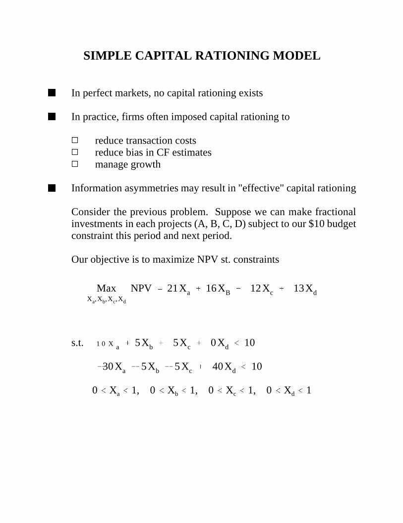
MaxXa,Xb,Xc,Xd

NPV ' 21Xa % 16XB % 12 Xc % 13Xd

SIMPLE CAPITAL RATIONING MODEL

2 In perfect markets, no capital rationing exists

2 In practice, firms often imposed capital rationing to

4 reduce transaction costs4 reduce bias in CF estimates4 manage growth

2 Information asymmetries may result in "effective" capital rationing

Consider the previous problem. Suppose we can make fractionalinvestments in each projects (A, B, C, D) subject to our $10 budgetconstraint this period and next period.

Our objective is to maximize NPV st. constraints

s.t. 1 0 X a % 5Xb % 5Xc % 0 Xd # 10

&30 Xa & 5Xb & 5 Xc % 40Xd # 10

0 # Xa # 1, 0 # Xb # 1, 0 # Xc # 1, 0 # Xd # 1

Solve using linear programming software (or trial and error)

Solution: Xa = .5, Xb = 1, Xc = 0, Xd = .75

NPV = $36.25 million (Increase of $2.25 million in NPV overinteger solution)

4 Sometimes fractional projects make sense (building size)

4 Sometimes project sizes need to occur in fixed increments &solve using integer (zero-one) programming

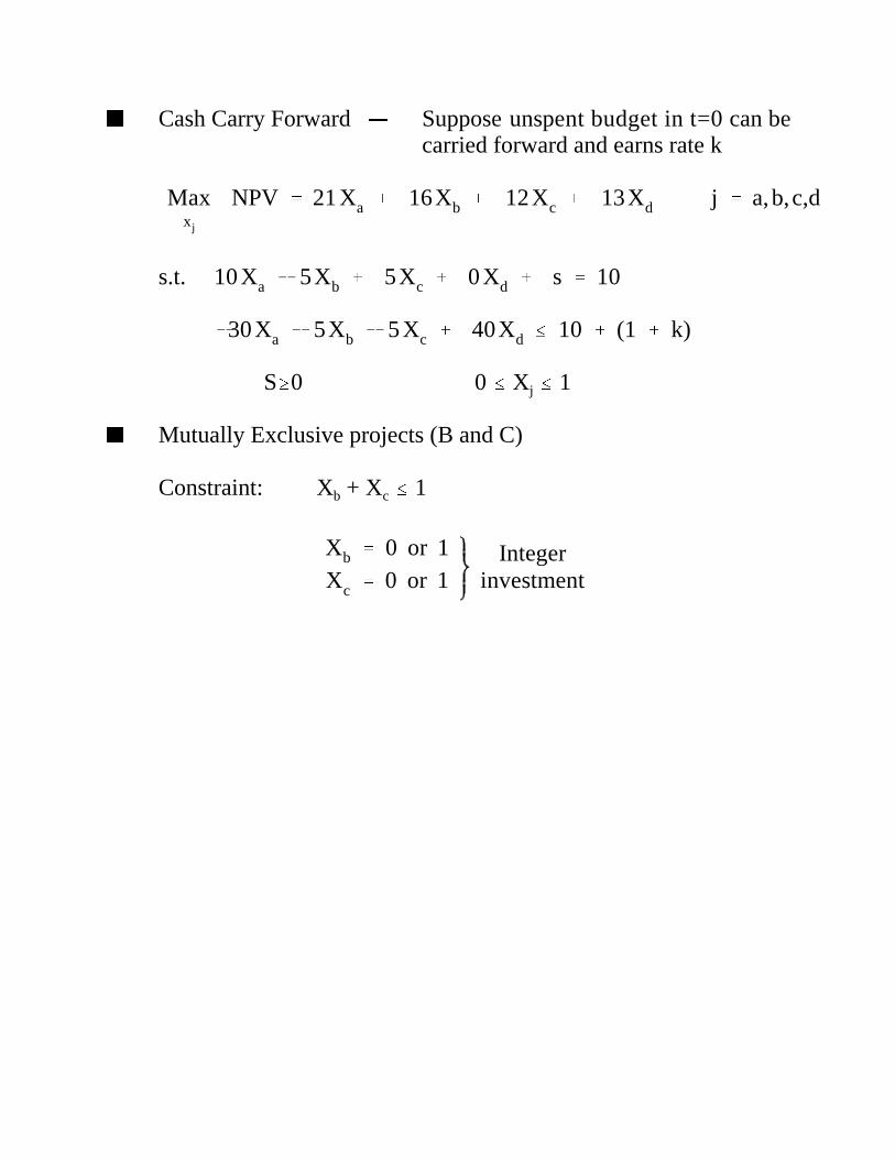
2 Cash Carry Forward & Suppose unspent budget in t=0 can becarried forward and earns rate k

Maxxj

NPV ' 21 Xa % 16Xb % 12Xc % 13Xd j ' a,b,c,d

s.t. 10 Xa & 5Xb % 5Xc % 0 Xd % s ' 10

&30 Xa & 5Xb & 5 Xc % 40Xd # 10 % (1 % k)

S$0 0 # Xj # 1

2 Mutually Exclusive projects (B and C)

Constraint: Xb + Xc # 1

Xb ' 0 or 1Xc ' 0 or 1

Integerinvestment

2 Contingent projects & Suppose D is attached to A. Can’taccept D without A.

Xa = 0 or 1

Xd = 0 or 1

Xd - Xa # 0

So,

if Xa = 1 Y Xd = 0 or 1Xa = 0 Y Xd = 0

2 Nonfinancial resource constraints

Suppose each project requires services of a 12 person supporttechnical design team

A = 3 FTE, B = 2 FTE, C = 8 FTE, D = 3 FTE

Constraint: 3Xa + 2Xb + 8Xc + 3Xd # 12

2 Could continue & many possible examples& L.P. is very versatile

2 Problems & difficult to justify constraints& difficult to deal with risk

u NPV(N, 4) ' NPV(N) (u % u 2% ä) (2)

NPV(N,4) ' NPV(N) (1 % u % u2 % ä) (1)

PROJECTS WITH DIFFERENT LIVES

Year C D k = 10%

0 (40,000) (20,000) Mutually Exclusive

1 8,000 7,000

2 14,000 13,000

3 13,000 12,000

4 12,000

5 11,000

6 10,000

NPVc = $9281 NPVd = 6123

2 Replication Method & assume projects can be replicated at aconstant scale

4 Compute NPV of an infinite stream of constant scalereplications

NPV(N, 4) = NPV(N) + + . . .NPV(N)

(1 % k)N%

NPV(N)

(1 % k)2N

Let u = 1

( 1 % k)N

N P V ( N , 4) & u NPV(N, 4) ' NPV(N)

NPV(N, 4) ' NPV(N)

1 & u' NPV(N) 1

1 &

1

(1 % k)N

' NPV(N)(1 % k)N

(1 % k)N& 1

This is the NPV of an N year project replicated at a constant scale oninfinite number of time.

NPVa(6, 4) = $9281 = $21,309.86(1 % .10)6

(1 % .10)6&1

NPVB(3, 4) = $6123 = $24,621.49(1 % .10)3

(1 % .10)3&1

B preferred under replication assumption.

Annual Equivalent Method (AE)

Calculate annuity amount a project’s NPV can provide during itslife.

NPV = AE(PVIFAk,n)

AE = = perpetual stream of incomeNPV

(PVIFAk,n) project could generate withreinvestment

Gives same answer as NPV (N, 4) if projects have same risk.

Problem may occur if projects have different risk (k).

NPV(N)

1 &

1

(1 % k)N

k

' k NPV(N)1

1 &

1

1 % k)n

AE ' kNPV(Nd,4)

Note: AE = = k NPV(N,4)NPV(N)

PVIFAk,n

Remember PVIFAk,n =

1 &

1

(1%k)N

kso

Suppose NPV (Nc) = NPV (Nd) but kc > kd

It is now possible that

NPV (Nc, 4) < NPV (N, 4)

but

kc NPV (Nc, 4) > kd NPV (Nd, 4)

So AE method may give the wrong result

Example

Year A B ka = 10% kb = 40%

0 -10 -10

1 6 6.55

2 6 6.55

3 6.55

NPVa = $0.4132 NPVb = $0.4074

NPVa (2,4) = .4132 = $2.3808(1.10)2

(1.10)2& 1

NPVb (3, 4) = .4074 = $0.641(1.40)3

(1.40)3& 1

ka NPVa (2, 4) = .10 (2.3808) = $0.23808

kb NPVb (3, 4) = .40 (.641) = $0.2564

B gives larger CF stream, but we can’t compare them directlybecause of different risk levels.

Note & we could have made other assumptions about how toreinvest. Our constant scale assumption look like

Year C D

0 (40,000) (20,000)

1 8,000 7,000

2 14,000 13,000

3 13,000 12,000 + (20,000)

4 12,000 7,000

5 11,000 13,000

6 10,000 12,000

NPVc = 9281 NPVd = 10,723

Other assumption

4 Other investments available in future

4 Scale of investment charges as CFs are received (remembercapital rationing example)

4 making no adjustment means funds are reinvested to earn k(i.e. NPV = 0)

2 Last thought on Projects With Unequal Lines

4 Could have made other assumptions about reinvestmentopportunities

4 If we make no reinvestment assumption, we are implicitlyassuming reinvestment in projects earning k (NPV = 0)

Example

Year D E D + E

0 (20,000) (20,000)

1 7,000 7,000

2 13,000 13,000

3 12,000 (34,770) (22,770)

4 3,477 3,477

5 3,477 3,477

6 38,247 38,247

FV of CFs from D

FV = 7000(1 + 10)2 + 13000(1 + .10)1 + 12000 = 34,770

NPVD+E = 6123

NPVD = 6123

NPVE = 0

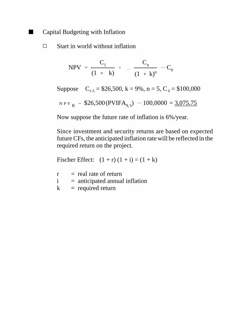
2 Capital Budgeting with Inflation

4 Start in world without inflation

NPV '

C1

(1 % k)% ä

Cn

(1 % k)n& C0

Suppose C1-5 = $26,500, k = 9%, n = 5, C 0 = $100,000

= 3,075.75N P V R ' $26,500(PVIFA9,5) & 100,0000

Now suppose the future rate of inflation is 6%/year.

Since investment and security returns are based on expectedfuture CFs, the anticipated inflation rate will be reflected in therequired return on the project.

Fischer Effect: (1 + r) (1 + i) = (1 + k)

r = real rate of returni = anticipated annual inflationk = required return

2 In our case

(1 % .09)(1 % .06) ' (1 % .09 % .06 % .0054)

Y k ' .1554 or 15.54%

Suppose you lend $1000 today and want to increase your purchasingpower next year by 9%.

Cost of goods and services next year = 1000 (1 + .06) = $1060

To increase purchases by 9% you need $1060 (1 + .09) = $1,155.40

Required return

r = - 1 = .1554 or 15.54%$1,155.40

1000

k = .09 + .06 + .0054 9 9 99% on 6% 9% on$1000 inflation inflation

amount

NPVN '

26,500(1 % .06)

(1 % .09)(1 % .06)% ä

26,500(1 % .06)5

(1 % .09)5 (1 % .06)5& 100,000

'

26,500

(1 % .09)% ä

26,500

(1 % .09)5& 100,000

' $3,078.75

2 Market data on interest rates and rates of return will include apremium for inflation that is anticipated.

To avoid bias 6 must include inflation effects in CFs.

Alternative: Don’t include inflation in CFs and remove inflationpremium from required return.

Suppose the 6% inflation rate applied to the projects CFs.

So NPVN = NPVR (NPV is both real and nominal)

NPV ' jn

j'1

(Rj (1 % iR)j& Ej (1 % iE)j

& Depj)(1 & t) % Depj

(1 % k)j& C0

2 Consistency:

1) Nominal CFs discounted at nominal rate2) Real CFs discounted at real rate

In practice, effect of inflation on CFs may differ from effect onrequired return.

Each of component may be impacted differently by expectedinflation.

4 Applications later

4 Point & account for anticipated inflation in CFs and discountrate.