ALTERNATIVE METHODS FOR CALCULATING OPTIMAL SAFETY …

ALTERNATIVE METHODS FOR CALCULATING

OPTIMAL SAFETY STOCK LEVELS

_______________________________________

A Thesis

presented to

the Faculty of the Graduate School

at the University of Missouri-Columbia

_______________________________________________________

In Partial Fulfillment

of the Requirements for the Degree

Master of Science

_____________________________________________________

by

ASHKAN MIRZAEE

Dr. Ronald McGarvey, Thesis Supervisor

MAY 2017

The undersigned, appointed by the Dean of the Graduate School, have examined the

thesis entitled:

ALTERNATIVE METHODS FOR CALCULATING

OPTIMAL SAFETY STOCK LEVELS

presented by Ashkan Mirzaee, a candidate for the degree of Master of Science and hereby

certify that, in their opinion, it is worthy of acceptance.

Dr. Ronald McGarvey

Dr. James Noble

Dr. Timothy Matisziw

Dr. Francisco Aguilar

ii

ACKNOWLEDGEMENTS

I would like to express my sincere gratitude to my advisor Dr. McGarvey for the

immeasurable amount of support and guidance he has provided throughout these years. Dr.

McGarvey’s patience and remarkable comments throughout this study have been

astonishingly invaluable. I would also like to thank my committee members Dr. Noble, Dr.

Matisziw and Dr. Aguilar who have given me support, assistance and inspiration. Special

recognition is given to the Industrial & Manufacturing Systems Engineering department

for their help and support.

I am especially grateful to my family for giving me the opportunity to follow my dreams

and the love to make them a reality. Furthermore, I would like to thank my friends at the

University of Missouri for their support and encouragement.

iii

TABLE OF CONTENTS

ACKNOWLEDGEMENTS ................................................................................................ ii

LIST OF TABLES .............................................................................................................. v

LIST OF FIGURES ........................................................................................................... vi

ABSTRACT ...................................................................................................................... vii

Chapter 1: Introduction and Literature Review .................................................................. 1

Chapter 2: Determination of Safety Stock Levels .............................................................. 5

2-1 Safety stock requirements ......................................................................................... 5

2-1-1 Cycle time .......................................................................................................... 6

2-1-2 Transit time ........................................................................................................ 6

2-1-3 Service level ....................................................................................................... 7

2-2 Traditional approach to calculate safety stock levels ............................................... 8

2-2-1 Expected value and standard deviation of lead time .......................................... 8

2-2-2 Expected value and standard deviation of demand rate ..................................... 9

2-2-3 Target inventory and actual demand ................................................................ 11

2-3 Alternative safety stock levels calculation .............................................................. 12

2-3-1 Service level adjustment .................................................................................. 12

2-3-2 Hybrid method ................................................................................................. 13

Chapter 3: Case Study Application ................................................................................... 16

iv

3-1 Analyzing safety stock requirements ...................................................................... 17

3-1-1 Cycle time ........................................................................................................ 17

3-1-2 Transit time ...................................................................................................... 17

3-2 Calculating safety stock levels by traditional approach .......................................... 18

3-2-1 Expected value and standard deviation of lead time ........................................ 18

3-2-2 Expected value and standard deviation of demand rate ................................... 19

3-2-3 Target inventory and actual demand ................................................................ 19

3-3 Alternative safety stock levels ................................................................................ 22

3-3-1 Using service level adjustment ........................................................................ 22

3-3-2 Using Hybrid method ....................................................................................... 25

Chapter 4: Conclusions and Further Study ....................................................................... 33

4-1 Conclusions ............................................................................................................. 33

4-2 Further study ........................................................................................................... 34

References ......................................................................................................................... 36

v

LIST OF TABLES

Table 1: Shortfalls service level adjustment ..................................................................... 24

Table 2: Comparing all methods across all wholesalers ................................................... 34

vi

LIST OF FIGURES

Figure 1: Direct sourced...................................................................................................... 7

Figure 2: Network sourced .................................................................................................. 7

Figure 3: Service level adjustment .................................................................................... 13

Figure 4: Gamma distribution ........................................................................................... 14

Figure 5: Shortfall distribution.......................................................................................... 20

Figure 6: Excess distribution ............................................................................................ 21

Figure 7: Normal vs. empirical ......................................................................................... 22

Figure 8: Normal service level adjustment ....................................................................... 23

Figure 9: Normal vs. Gamma............................................................................................ 25

Figure 10: Hybrid-1 results ............................................................................................... 26

Figure 11: Hybrid-1 vs Normal......................................................................................... 26







Figure 18: Hybrid method results ..................................................................................... 31

vii

ABSTRACT

This work considers the problem of safety stock levels for the production of multiple items,

each with random demand, across multiple facilities. The traditional methodology for

calculating safety stock is discussed and an alternative method for improving service

levels is offered. Normal and Gamma distributions are considered to estimate safety stock

levels, and the performance of both models, along with a hybrid approach, are tested on a

large-scale case study example. The results of this case study indicate that a better

inventory policy with less underage and overage cost can be achieved by using the

proposed model and solution procedure.

1

Chapter 1: Introduction and Literature Review

Introduction and Literature Review

In today’s logistics, inventory control plays a crucial role in supply chain management in

order to achieve a reliable and efficient supply network. Inventory control is a common

problem in different sectors which illustrates how modern life is dependent upon the larger

network supplying materials, products and goods. Supply chain variables such as demand,

lead time, production time and transportation cost fluctuate due to random perturbations

and the nature of the environment. A responsive inventory control can provide a cushion

against the variations of these variables. Many different studies have examined different

aspects of the relationship between variability and inventory control.

Brander and Forsberg (2006) considered the problem of inventory and scheduling the

production of multiple items, each with random demand, on a single facility and presented

a model for determination of safety stocks, order-up-to levels and an estimation method for

the variance in demand during lead time. Gallego (1990) applied a simulation-based search

method for calculating safety stock levels for random demands with constant expected

rates. Bourland and Yano (1994) used cyclic schedules for inventory management and

developed a planning and control model. They offered a nonlinear mathematical program

for determining the cycle length, allocation of idle times, and safety stock levels. Smits et

al. (2004) offered a method based on queuing analysis to determine order-up-to levels for

a (R, S) system and a fixed cyclic production sequence, where the demand is a compound

of renewal process. Sox et al. (1999) presented a method for determination of safety stock

levels in models where the production and inventory control are constructed

2

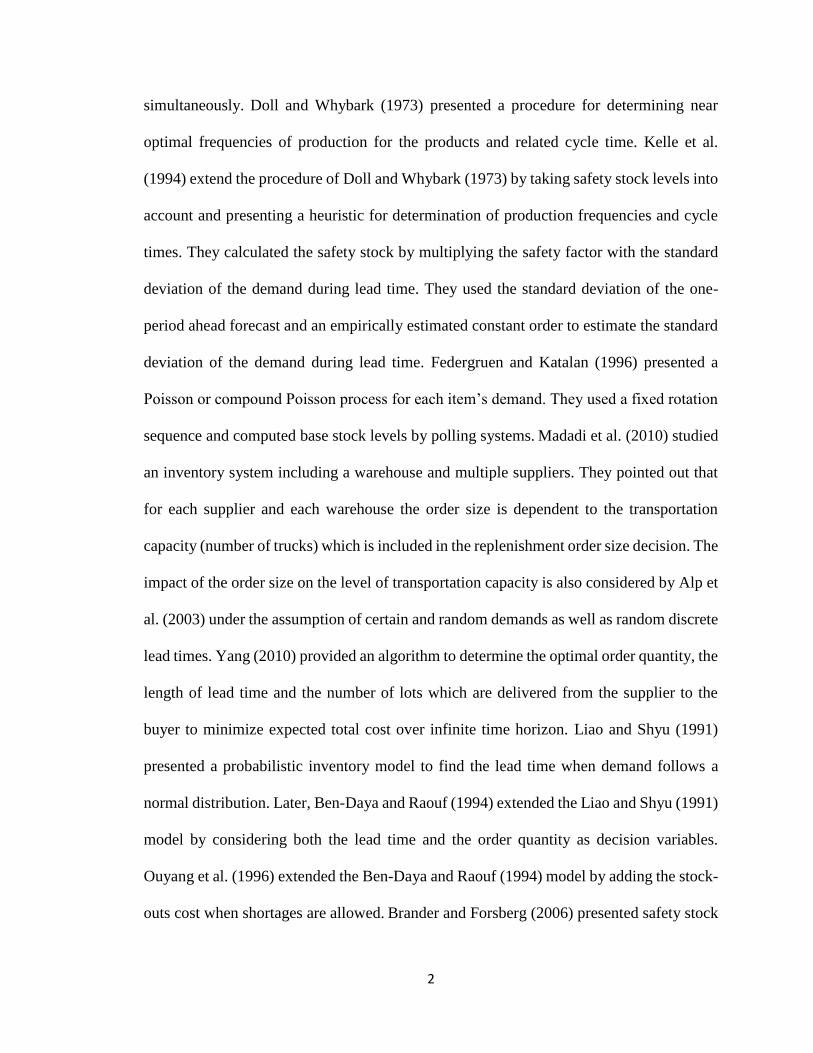
simultaneously. Doll and Whybark (1973) presented a procedure for determining near

optimal frequencies of production for the products and related cycle time. Kelle et al.

(1994) extend the procedure of Doll and Whybark (1973) by taking safety stock levels into

account and presenting a heuristic for determination of production frequencies and cycle

times. They calculated the safety stock by multiplying the safety factor with the standard

deviation of the demand during lead time. They used the standard deviation of the one-

period ahead forecast and an empirically estimated constant order to estimate the standard

deviation of the demand during lead time. Federgruen and Katalan (1996) presented a

Poisson or compound Poisson process for each item’s demand. They used a fixed rotation

sequence and computed base stock levels by polling systems. Madadi et al. (2010) studied

an inventory system including a warehouse and multiple suppliers. They pointed out that

for each supplier and each warehouse the order size is dependent to the transportation

capacity (number of trucks) which is included in the replenishment order size decision. The

impact of the order size on the level of transportation capacity is also considered by Alp et

al. (2003) under the assumption of certain and random demands as well as random discrete

lead times. Yang (2010) provided an algorithm to determine the optimal order quantity, the

length of lead time and the number of lots which are delivered from the supplier to the

buyer to minimize expected total cost over infinite time horizon. Liao and Shyu (1991)

presented a probabilistic inventory model to find the lead time when demand follows a

normal distribution. Later, Ben-Daya and Raouf (1994) extended the Liao and Shyu (1991)

model by considering both the lead time and the order quantity as decision variables.

Ouyang et al. (1996) extended the Ben-Daya and Raouf (1994) model by adding the stock-

outs cost when shortages are allowed. Brander and Forsberg (2006) presented safety stock

3

levels based on estimation of the standard deviation in total demand during a replenishment

lead time. If lead time and demand are assumed to be independent random variables the

standard deviation in total demand is dependent on the variance and mean of demand and

lead time (Ross 1983). Inderfurth and Vogelgesang (2013) considered safety stock

problems under stochastic demand and production yield. Braglia et al. (2016) studied a

single-vendor single-buyer supply chain problem under continuous review and Gaussian

lead-time demand. Moncayo-Martínez and Zhang (2013) considered a heuristic method

and Pareto optimality criterion for finding the economic order quantity and safety stock

level.

Applications of inventory theory often rely on the normal distribution but there are many

other probability density functions (PDF) for statistical description of the demand

process. Fortuin (1980) compared five different pdf's (Gaussian, logistic, gamma, log-

normal, Weibull) for demand process. Snyder (1984) used the gamma probability

distribution in order to cover normal distribution as special cases and also cover the gaps

left by this distribution. Chopra et al. (2004) considered safety stocks for gamma lead

times and different service levels. Chaturvedi and Martínez‐de‐Albéniz (2016) found

safety stock levels when demand and capacity are gamma distributed.

This work considers the problem of safety stock levels of the production of multiple items,

each with random demand, on multiple facilities. The rest of this thesis is organized as

follows. In the next chapter, the traditional method for calculating safety stock levels is

discussed. The traditional approach, which is referred as the Normal method, assumes that

demand during lead time is normally distributed. Moreover, two alternative approaches for

non-normal shape probability distributions are introduced in this chapter. In Chapter 3, a

case study is described and conducted to demonstrate the performance of the suggested

4

methods. Chapter 4 presents conclusions from the results of the case study and suggests

potential future research extensions.

5

Chapter 2: Determination of Safety Stock Levels

Determination of Safety Stock Levels

Inventory control is a problem common to many organizations in different sectors.

Inventories are found at manufacturers, wholesalers, retailers, farms, hospitals, universities

and governments and are relevant to food, medicines, clothing, and many other areas.

Inventory may consist of supplies, raw materials, in-process goods, and finished goods.

Generally, the term inventory can be used to describe stock on hand at a given time. Risk

and uncertainty impact inventory analysis through many variables, but the most dominant

are uncertainty in demand and lead time. Such variations can be absorbed by provision of

safety stocks. Safety stocks are inventory in excess of average demand that are kept on

hand to avoid stock-outs due to uncertainty in demand and lead time. They are needed to

cover the demand during the replenishment lead time in case actual demand exceeds

expected demand, or the lead time exceeds the expected lead time. Safety stock calculations

are based, in part, on sales forecasts. Since forecasts are seldom exactly correct, the safety

stock protects against higher than expected demand levels. Safety stock has two effects on

a firm’s cost: it decreases the cost of stock-outs, but it increases holding costs (Tersine

1994).

2-1 Safety stock requirements

More formally, the term safety stock in supply chain and logistics is used for describing a

level of extra stock that is maintained to mitigate risk of stock-outs (shortfall) due to

uncertainties in supply and demand. Safety stock act as a buffer stock in case the sales are

greater than planned and or the supplier is unable to deliver the additional units at the

6

expected time. Safety stock is a function of the production cycle time and transportation

time, increasing variability in production and delivery time will increase shortfall risk.

Given a desired service level, safety stock calculation must consider the trade-off between

holding cost and stock-outs cost.

2-1-1 Cycle time

Manufacturing cycle time (𝐶) refers to the time required or spent to convert raw materials

into finished goods. In this study, 𝐶 is a random variable with mean 𝜇𝐶 and standard

deviation 𝜎𝐶 which refers to the time from the start of production to the finish of the final

products. It is usually composed of process time, move time, inspection time, and queue

time.

2-1-2 Transit time

Transportation plays a vital role in supply chain management. This element not only

generates cost in a distribution network, but contributes significantly to the quality of

customer service (Tyworth and Zeng 1998). The transit time includes the travelling time

from origin to destination. The transit time may change, particularly when the destination

is not reached directly but via several hubs.

In general, products could be sourced in two ways, first directly from the manufacturer

(Figure 1) and second via distribution centers (Figure 2). Although more complicated

situations for transporting products that include travel through multiple distribution centers

(DCs) are possible, in this study we consider only these two mentioned possibilities. For

directly sourced products the transit time is equal to the transit time between manufacturer

and wholesaler (𝑇1) with mean 𝜇𝑇1standard deviation 𝜎𝑇1.

7

Figure 1: Direct sourced

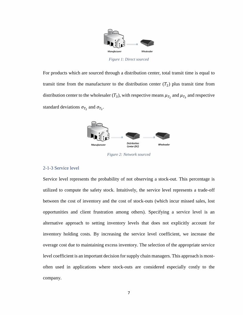
For products which are sourced through a distribution center, total transit time is equal to

transit time from the manufacturer to the distribution center (𝑇2) plus transit time from

distribution center to the wholesaler (𝑇3), with respective means 𝜇𝑇2 and 𝜇𝑇3 and respective

standard deviations 𝜎𝑇2 and 𝜎𝑇3.

Figure 2: Network sourced

2-1-3 Service level

Service level represents the probability of not observing a stock-out. This percentage is

utilized to compute the safety stock. Intuitively, the service level represents a trade-off

between the cost of inventory and the cost of stock-outs (which incur missed sales, lost

opportunities and client frustration among others). Specifying a service level is an

alternative approach to setting inventory levels that does not explicitly account for

inventory holding costs. By increasing the service level coefficient, we increase the

overage cost due to maintaining excess inventory. The selection of the appropriate service

level coefficient is an important decision for supply chain managers. This approach is most-

often used in applications where stock-outs are considered especially costly to the

company.

8

2-2 Traditional approach to calculate safety stock levels

The traditional approach, which we refer to the Normal method, assumes that demand

during lead time is normally distributed, with mean 𝜇𝑥 and standard deviation 𝜎𝑥 (Brander

and Forsberg 2006; Silver et al. 1998). The safety stock level of item 𝑥 (for one certain

product in a certain wholesaler) is equal to:

𝑆𝑆𝑥 = 𝜎𝑥Φ−1(𝜋𝑥) (1)

where 𝜎𝑥 is the standard deviation of total demand during lead time for item 𝑥 and Φ−1(𝜋𝑥)

is the standard normal inverse cumulative density function (CDF) at 𝜋𝑥 service level.

Observe that any inverse CDF could be used here to compute Φ−1(𝜋𝑥), the normal

distribution is just the one typically selected. In order to calculate safety stock levels from

(1), we need to estimate 𝜎𝑥, the standard deviation of the demand during lead time. Ross

(1983) showed if lead time and demand are assumed to be independent random variables,

the standard deviation of demand during lead time, 𝜎𝑥, is equal to:

𝜎𝑥 = √𝜇𝐿𝜎𝐷2 + 𝜇𝐷2𝜎𝐿2 (2)

Where 𝜇𝐿 and 𝜎𝐿 are the expected value and standard deviation of lead time and 𝜇𝐷 and 𝜎𝐷

are the expected value and standard deviation of demand rate for item 𝑥.

2-2-1 Expected value and standard deviation of lead time

Expected lead time (𝜇𝐿) is equal to the average transit times between sites plus the cycle

time for product 𝑥 at its manufacturer. 𝜇𝐿 is calculated as:

9

𝜇𝐿 = {

𝜇𝑇1 + 𝜇𝐶 , 𝑖𝑓 𝑠𝑜𝑢𝑟𝑐𝑒𝑑 𝑓𝑟𝑜𝑚 𝑚𝑎𝑛𝑓𝑎𝑐𝑡𝑢𝑟𝑒𝑟

𝜇𝑇2 + 𝜇𝑇3 + 𝜇𝐶 + 𝜇𝑆, 𝑖𝑓 𝑠𝑜𝑢𝑟𝑐𝑒𝑑 𝑓𝑟𝑜𝑚 𝐷𝐶 (3)

Where 𝜇𝑆 is the mean of the additional time item 𝑥 spends sitting at the distribution center.

Standard deviation of lead time (𝜎𝐿) is equal to square root of the variance of transit times

between sites plus the variance of production cycle time. 𝜎𝐿 is calculated by:

𝜎𝐿 =

{

√𝜎𝑇12 + 𝜎𝐶

2 , 𝑖𝑓 𝑠𝑜𝑢𝑟𝑐𝑒𝑑 𝑓𝑟𝑜𝑚 𝑚𝑎𝑛𝑓𝑎𝑐𝑡𝑢𝑟𝑒𝑟

√𝜎𝑇22 + 𝜎𝑇3

2 + 𝜎𝐶2 + 𝜎𝑆

2 , 𝑖𝑓 𝑠𝑜𝑢𝑟𝑐𝑒𝑑 𝑓𝑟𝑜𝑚 𝐷𝐶

(4)

Where 𝜎𝑆2 is the variance of the additional time item 𝑥 spends sitting at the distribution

center.

2-2-2 Expected value and standard deviation of demand rate

Assume that forecasts are available for weekly sales. Expected demand rate 𝜇𝐷 is equal to

the total expected (forecasted) demand during expected lead time divided by the lead time.

If lead time is computed in days, we can separate the expected lead time into its integer

(𝓌) and fractional (𝓇) components as follows:

𝓌 = ⌊𝜇𝐿7⌋ (5)

𝓇 = 𝜇𝐿 − (𝓌 ∗ 7) (6)

10

Let 𝐹𝐶𝑆𝑇𝑗 denote the forecast demand during week 𝑗, and let 𝐷𝐴𝑌𝑖 denote the percentage

of a typical week’s demand that is observed on day 𝑖. Then, we can compute the percentage

of a typical week’s demand associated with 𝓇 days, denoted ℛ, as follows:

ℛ =∑𝐷𝐴𝑌𝑖

⌊𝓇⌋

𝑖=1

+ (𝓇 − ⌊𝓇⌋) ∗ 𝐷𝐴𝑌⌊𝓇⌋+1 (7)

Assume that the current time is the beginning of week 1. Then expected demand rate 𝜇𝐷

can be computed as:

𝜇𝐷 =

{

1

𝜇𝐿(ℛ ∗ 𝐹𝐶𝑆𝑇1), 𝓌 = 0

1

𝜇𝐿[∑(𝐹𝐶𝑆𝑇𝑗

𝓌

𝑗=1

) + ℛ ∗ 𝐹𝐶𝑆𝑇𝓌+1] , 𝓌 > 0

(8)

Because the forecast demand can vary greatly from week to week, it is typically assumed

that the distribution of demand is not stationary across weeks. As a result, in practice it is

common to replace the standard deviation of the demand rate 𝜎𝐷 in equation (2) with the

root-mean-square error (𝑅𝑀𝑆𝐸), a measure of forecast accuracy. Given historical data for

the actual sales quantity in week 𝑗, denoted 𝑆𝑄𝑗, the square error for week 𝑗, denoted 𝑆𝐸𝑗,

is computed as:

𝑆𝐸𝑗 = (𝐹𝐶𝑆𝑇𝑗 − 𝑆𝑄𝑗)2 (9)

𝑅𝑀𝑆𝐸 can thus be computed over a historical interval of 𝑚 weeks as follows:

𝑅𝑀𝑆𝐸 = √1

m ∗ 7∑𝑆𝐸𝑗

𝑚

𝑗=1

(10)

11

We will then substitute 𝜎𝐷 = 𝑅𝑀𝑆𝐸 in all safety stock calculations.

2-2-3 Target inventory and actual demand

The target inventory of item 𝑥 at the start of an arbitrary week is thus equal to the safety

stock level, 𝑆𝑆𝑥, plus the expected demand during the lead time, 𝜇𝑥. In other words, target

inventory 𝑇𝐼𝑥 is:

𝑇𝐼𝑥 = 𝜇𝑥 + 𝑆𝑆𝑥 (11)

Where expected demand during the lead time is equal to the expected demand rate from

equation (8) multiplied by the expected lead time from equation (3):

𝜇𝑥 = 𝜇𝐷𝜇𝐿 (12)

Therefore, if we assume that demand during lead time follows a normal distribution, then

target inventory is equal to:

𝑇𝐼𝑥 = 𝜇𝑥 + 𝜎𝑥Φ−1(𝜋𝑥) = Φ𝜇𝑥,𝜎𝑥2

−1 (𝜋𝑥) (13)

Where Φ𝜇𝑥,𝜎𝑥−1 (𝛼𝑥) is the normal inverse CDF with mean of 𝜇𝑥 and standard deviation of

𝜎𝑥, at given service level 𝜋𝑥.

Note that, by assuming a constant lead time (value of zero for standard deviation of lead

time) and given actual sales quantities 𝑆𝑄𝑗 for week 𝑗 we can compute the actual demand

during the lead time, denoted 𝐴𝐷𝑥, as follows:

𝐴𝐷𝑥 =

{

ℛ ∗ 𝑆𝑄𝑗, 𝓌 = 0

(∑𝑆𝑄𝑗

𝓌

𝑗=1

) + ℛ ∗ 𝑆𝑄𝓌+1 , 𝓌 > 0

(14)

12

Observe that if 𝐴𝐷𝑥 is greater than 𝑇𝐼𝑥, then a shortfall (stock-out) would have occurred

under target inventory 𝑇𝐼𝑥.

2-3 Alternative safety stock levels calculation

The traditional (Normal) method could be a practical way to set target inventories for

problems if demand follows a normal probability distribution, but it is unclear if the Normal

approach would work well in situations where demand does not follow a normal

distribution. In this thesis, we proposed two methods to find a better-performing safety

stock calculation for problems with non-normally distributed demand. The first is Service

level adjustment and the other one is Hybrid method.

2-3-1 Service level adjustment

Consider a notional set of demand data as presented in the histogram of Figure 3. We can

compute the mean and standard deviation of these data, and have overlaid a curve showing

the probability density function (PDF) of a normal distribution with this same mean and

standard deviation. Suppose our desired service level was 𝜋𝑥 = 0.95. In Figure 3 the blue

line represents the demand level associated with a 95 percent service level, based on the

PDF of the normal distribution (Φ−1(0.95) = 5.15). The red line in the figure shows the

actual demand level of the empirical data associated with service level 𝜋𝑥 = 0.95

(F−1(0.95) = 5.53). Observe that basing the safety stock on the Normal method would

lead to stock-outs more frequently than the target 1 − 𝜋𝑥 = 5 percent of the time, since

demand level 5.15 is associated with empirical cumulative distribution function (CDF)

value of 0.93. Because the demand level of 5.53 was associated with 5% stock-outs in the

empirical data, the service level adjustment approach would simply use the Normal

method, but increase the target service level parameter 𝜋𝑥 to be equal to the CDF value

13

Φ(5.53) = 0.97. That is, we would aim to achieve 5% stock-outs by basing our target

inventory on 𝜋𝑥 = 0.97.

Figure 3: Service level adjustment

2-3-2 Hybrid method

The Hybrid method utilizes a combination of historical and forecast-based data. Instead of

assuming that the demand during lead time follows a normal distribution, we instead

assume that this demand can be represented by a Gamma distribution, which is much more

flexible. The Gamma distribution is specified by two parameters, the shape (𝛼) and rate

(𝛽). The mean and standard deviation of a Gamma distribution are given by 𝛼

𝛽 and

√𝛼

𝛽,

respectively. Figure 4 shows a Gamma distribution with the same mean and standard

deviation as the empirical data, overlaid on the empirical histogram. Observe that the

Gamma distribution appears to fit the data much better than does the normal distribution.

14

Figure 4: Gamma distribution

Because of the distribution of demand across time is assumed to not be stationary across

weeks, we may not want to base our estimates of the mean and standard deviation of

demand solely on historical data. Instead, must like the Normal method (which uses a

forecast-based mean and a historical-based 𝑅𝑀𝑆𝐸 for the standard deviation), our Hybrid

method will fit the Gamma distribution shape and rate parameters based on a combination

of historical and forecast-based data. We will consider all four possible combinations:

▪ Historical-based shape and historical-based rate

▪ Forecast-based shape and forecast-based rate

▪ Historical-based shape and forecast-based rate

▪ Forecast-based shape and historical-based rate

As an example, consider again the data presented in Figures 3 and 4. This notional data has

a mean of 𝜇 = 2.5 and standard deviation of 𝜎 = 1.56. Assume further that the forecast

demand during lead time 𝜇𝑥 is equal to 5 and the 𝑅𝑀𝑆𝐸 estimate of 𝜎𝐷 was equal to 2. Our

proposed approach would calculate the Gamma distribution parameters as follows:

15

▪ Historical-based shape and historical-based rate:

𝛼 =𝜇2

𝜎2= 2.43; 𝛽 =

𝜇

𝜎2= 1.03

▪ Forecast-based shape and forecast-based rate:

𝛼 =𝜇𝑥2

𝑅𝑀𝑆𝐸𝑥2= 6.25; 𝛽 =

𝜇𝑥𝑅𝑀𝑆𝐸𝑥2

= 1.25

▪ Historical-based shape and forecast-based rate

𝛼 =𝜇2

𝜎2= 2.43; 𝛽 =

1

2(𝛼

𝜇𝑥+√

𝛼

𝑅𝑀𝑆𝐸𝑥2) = 0.63

▪ Forecast-based shape and historical-based rate

𝛽 =𝜇

𝜎2= 1.03; 𝛼 =

1

2(𝜇𝑥𝛽 + 𝑅𝑀𝑆𝐸𝑥

2𝛽2) = 4.70

Under each combination, we can specify the PDF of the demand during lead time by using

the Gamma distribution PDF: 𝑓(𝑥) =𝛽𝛼

Γ(α)𝑥𝛼−1𝑒−𝛽𝑥, where Γ(α) is the Gamma function

∫ 𝑥𝛼−1𝑒−𝑥∞

0𝑑𝑥. The target inventory can then be calculated from equation (13), assuming

that 𝑇𝐼𝑥 is equal to the inverse CDF of the appropriate Gamma distribution.

16

Chapter 3: Case Study Application

Case Study Application

We partnered with a liquid consumer packaged goods company to examine a case study

applying these alternative inventory requirement calculations. This liquid consumer

packaged goods company operates a set of production facilities companies which are

supporting a set of more than 500 wholesalers. Each wholesaler has an inventory of

products supporting its sales to retail locations. For each product that is carried at a given

wholesaler, the service level target is to have stock-outs no more than 0.22% of the time.

In practice, the company observed that stock-outs occur more frequently than this target

level.

Problem context:

Three-week-out distribution plans are made, aiming to keep wholesaler inventory at the

target inventory level three weeks from the current date, based on forecast demands, such

that a service level target is achieved. Note that different production facilities produce

various products with different cycles, for example, some products are only produced every

four weeks and others produced every week. Moreover, some wholesalers receive some

products directly shipped from the company, while other products are received from a

distribution center.

Approach:

Identify frequency of shortfall occurrence using historical data, had target inventories been

computed using Normal method. Calculate how much additional safety stock would have

17

been needed to achieve desired performance. Determine if alternative Hybrid method could

have achieved better performance than the Normal method, with respect to service level

achieved, relative to target service level.

Output:

Alternative safety stock requirements that can be implemented in existing inventory

management systems.

3-1 Analyzing safety stock requirements

We obtained files from the company providing sales quantity and forecasted demand for

certain products, at each wholesaler, for each week over a 15-month period. The database

includes records across a set of nearly 250,000 unique product-wholesaler pairs.

3-1-1 Cycle time

In order to compute safety stocks, we need to identify the production cycle associated with

each product-production facility pair. The available data provided a single cycle time (𝐶),

in weeks, for each pair. A constant standard deviation of 2.5 days was assumed for all

product-production facility pairs cycle times.

3-1-2 Transit time

The company’s products are sourced in two ways, first directly from production facilities

(Figure 1) and second, via distribution centers (Figure 2). For directly sourced pairs the

transit time is equal to the average transit time between a production facility-wholesaler

pair (𝑇1). The data also provided the transit time standard deviation (𝜎𝑇1) for production

facility-wholesaler pairs. When transit times were missing from the data, we estimated the

18

values from other shipments from the production facility to other wholesalers in the same

state.

For network sourced pairs, total transit time is equal to the transit time from the production

facility to the utilized distribution center (𝑇2) plus the transit time from the DC to the

wholesaler (𝑇3). This same data set also contained means and standard deviations for transit

times between production facilities and DCs, and between DCs and wholesalers. Due to

limitations on available data for production cycle frequencies and transit times, our analysis

was able to consider approximately 93% of the total sales, as measured by volume, across

this data set.

3-2 Calculating safety stock levels by traditional approach

Based on the traditional approach, demand during the lead time is assumed to be distributed

normally with standard deviation 𝜎𝑥. Given desired service level 𝜋𝑥 = 99.78% for all

products, the safety stock 𝑆𝑆𝑥,𝑘 for product 𝑥 in week 𝑘 is equal to:

𝑆𝑆𝑥,𝑘 = 𝜎𝑥,𝑘Φ−1(0.9978) = 2.85𝜎𝑥,𝑘 (15)

where 𝜎𝑥,𝑘 is the standard deviation of the total demand during lead time for item 𝑥 in week

𝑘, as calculated by equation (2).

3-2-1 Expected value and standard deviation of lead time

We assumed a single production cycle for each product-production facility pair, and a

single transit time average between each pair of locations, these values are not assumed to

change across different weeks. Also, we assumed the mean of the additional time which

item 𝑥 spends sitting at the distribution center is zero (𝜇𝑆 = 0). We can then compute the

value of 𝜇𝐿 for each product-wholesaler pair using equation (3).

19

Because we assume that the standard deviation of production cycle time is equal to 2.5

days for all product-production facility pairs, and the standard deviation of the additional

delay due to sitting at a DC is 2 days, we can calculate 𝜎𝐿 using equation (4), simplified as:

𝜎𝐿 =

{

√𝜎𝑇12 + 6.25 , 𝑠𝑜𝑢𝑟𝑐𝑒𝑑 𝑓𝑟𝑜𝑚 𝑚𝑎𝑛𝑢𝑓𝑎𝑐𝑡𝑢𝑟𝑒𝑟

√𝜎𝑇22 + 𝜎𝑇3

2 + 6.25 + 4 , 𝑠𝑜𝑢𝑟𝑐𝑒𝑑 𝑓𝑟𝑜𝑚 𝐷𝐶

(16)

3-2-2 Expected value and standard deviation of demand rate

The expected demand rate for each product-wholesaler pair at a certain date is calculated

by equation (8). Note that because the company utilizes three-week-out distribution plans,

𝐹𝐶𝑆𝑇1 here refers to the forecast demand for the week three weeks from the current time,

𝐹𝐶𝑆𝑇2 here refers to the forecast demand for the week four weeks from the current time,

etc.

Since three-week-out distribution plans are made and historical sales quantity and

forecasted demand are available, we compute 𝜎𝐷 as equal to the root-mean-square error

(𝑅𝑀𝑆𝐸) of three-week-out forecast versus actual sales in week 𝑘 over the previous 52

weeks for each product-wholesaler pair using equation (10), with 𝑚 = 52.

3-2-3 Target inventory and actual demand

Given the expected lead times for each product-wholesaler pair, we computed the actual

demand during the lead time for each week from historical sales records, as in equation

(14). We first evaluated the performance of the Normal method, computing target

inventory levels based on equation (13), where, as noted previously, Φ−1(0.9978) = 2.85

20

for all product-wholesaler pairs. Across the set of more than 5 million records analyzed,

we observed the following performance.

At 99.78% service level (i.e., 𝑍 = 2.85):

▪ Records with Shortfall = 0.75%

▪ Records with Excess = 99.16%

▪ Records with Equal actual demand and target inventory = 0.09%

Examining the quantities of shortfall and excess:

▪ Average of Shortfall = ℬ liters

▪ Average of Excess = 3.42ℬ liters

Observe that the desired 99.78% service level implies stock-outs should occur 0.22% of

the time, but our analysis suggests stock-outs would have occurred more than three times

as often (0.75%), across this set of records.

The following histograms show the distribution of shortfalls based on the volume of

shortage that we compute would have occurred. Figure 5a shows that the preponderance of

shortfalls occurred for deficit of ℬ liters or less and Figure 5b reveals that there are a few

records in the tail of the distribution with rare frequencies and high volume.

Figure 5: Shortfall distribution 5a 5b

𝑦

Shortfall Vol ℬ 100ℬ

𝑦

500

Shortfall Vol

21

The histograms in the figure below show the distribution of excess based on the volume of

excess that we compute would have occurred across this record set.

Figure 6: Excess distribution

Under the Normal method, safety stock is equal to 2.85 times the standard deviation of

demand during the lead time. The actual demand during lead time should be less than target

inventory 99.78% of the time, if demand during lead time follows a normal distribution.

Figure 7 shows a histogram of all empirical data for demand during lead time versus the

corresponding normal distribution with the same mean and standard deviation. Observe

that the normal distribution does not show a good fit for the data set. In particular, the fit

for the right-tail of the distribution, which is the area of greatest interest, since we are most

concerned with stock-outs, is poorly the by the normal distribution. Assuming the CDF of

the normal distribution implies a target inventory of ℒ liters (Φ𝜇𝜎2−1 (0.9978) = ℒ) while

under the empirical distribution’s CDF, a service level of 99.78% would require 2.67ℒ

liters (𝐹−1(0.9978) = 2.67ℒ). A substantial increase in the target inventory levels would

be needed for this example to achieve the desired service level.

6a 6b

Excess Vol Excess Vol

100𝑦

5ℬ 500ℬ

𝑦

125

22

Figure 7: Normal vs. empirical

3-3 Alternative safety stock levels

We observed that the Normal method, assuming a normal distribution for the demand

during lead time, can perform poorly when the demand is not normally-distributed. This

study offers two methods to try to improve the performance of target inventories. The first

method to attempt to reach the company’s desired service level is service level adjustment,

which is discussed under section 3-3-1. We will also examine a Hybrid method under

section 3-3-2.

3-3-1 Using service level adjustment

The company’s goal is satisfying a desired service level which implies that stock-outs occur

no more than 0.22% of the time. Increasing the target service level under an assumed

normal distribution could potentially make up this deficiency. We first examined the

performance of uniform changes to the Z-value, 𝑍 = Φ−1(𝜋𝑥), across all records in our

data set. As presented in Figure 8 the Normal method assumes 𝑍 = 2.85, and achieves an

overall performance of 0.75% shortfalls, as discussed in section 3-2-3. If we increase the

Actual demand during lead time

Φ𝜇𝜎2(ℒ) = 0.9978 𝐹(2.67ℒ) = 0.9978

23

Z-value to 3.25 for all safety stock calculations, the percentage of shortfalls decreases to

0.50%. In order to achieve the desired service level of 0.22% shortfalls, we need to increase

the Z-value to 4.3. Note that, from the normal distribution CDF, Φ−1(0.999991) = 4.3,

which suggests that the Normal method would expect that such a large inventory level

would only observe 0.0009% stock-outs. The results under this 𝑍 = 4.3 service level

adjustment are as follows:

▪ Records with Shortfall = 0.22%

▪ Records with Excess = 99.76%

▪ Average of Shortfall = 1.40ℬ liters

▪ Average of Excess = 5.1ℬ liters (average of excess inventory has increased by 49%,

relative to current baseline with 𝑍 = 2.85)

Figure 8: Normal service level adjustment

Performing this analysis across all product-wholesaler combinations masks the variance

between combinations. It is possible that the necessary increases in inventory might differ

across different types of product-wholesaler pairs. The company has an existing

classification that separates products into eleven families of products (segments). We can

24

perform a similar analysis for each segment at each wholesaler, identifying the Z-value

necessary to achieve 0.22% shortfalls for all data records in that segment. Table 1 shows

the shortfall percentage at Z-value = 2.85 in a certain wholesaler and the Z-value necessary

to achieve no more than 0.22% shortfalls for all data records these segments.

Table 1: Shortfalls service level adjustment

Segment %Shortfall

Z=2.85

Z-value

New

%Shortfall

Z New

Segment A 1.30% 4.05 0.00%

Segment C 0.38% 3.95 0.19%

Segment F 2.07% 4.15 0.19%

Segment G 1.79% 6.05 0.18%

Segment H 0.51% 3.35 0.17%

Segment I 1.79% 5.65 0.00%

Segment J 0.61% 3.25 0.00%

Segment K 0.26% 3.05 0.13%

The metric the company is using accepts an overall shortfall percentage of 0.22%, it would

potentially allow all the shortfalls to occur in one segment, and no shortfalls in any other

segment, as long as the aggregate metrics are met.

Unfortunately, this Service level adjustment process is very time-consuming, since one has

to examine a range of potential Z-values, updating all calculations for each new Z-value,

in order to identify the smallest Z-value that achieves the desired service level (as in Figure

8). The desire to find a procedure that is less computationally expensive, and which can

thus be easily extended to any number of segments, led to the creation of the Hybrid

method, examined in the next section.

25

3-3-2 Using Hybrid method

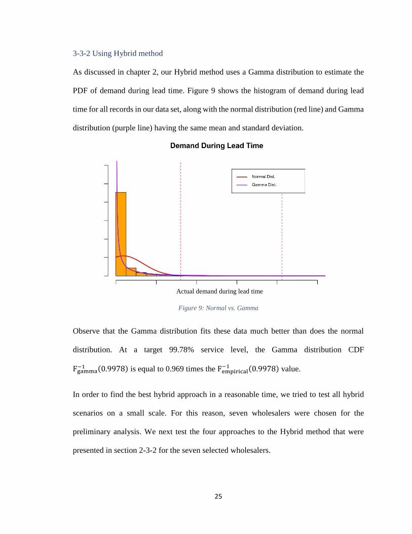
As discussed in chapter 2, our Hybrid method uses a Gamma distribution to estimate the

PDF of demand during lead time. Figure 9 shows the histogram of demand during lead

time for all records in our data set, along with the normal distribution (red line) and Gamma

distribution (purple line) having the same mean and standard deviation.

Figure 9: Normal vs. Gamma

Observe that the Gamma distribution fits these data much better than does the normal

distribution. At a target 99.78% service level, the Gamma distribution CDF

Fgamma−1 (0.9978) is equal to 0.969 times the Fempirical

−1 (0.9978) value.

In order to find the best hybrid approach in a reasonable time, we tried to test all hybrid

scenarios on a small scale. For this reason, seven wholesalers were chosen for the

preliminary analysis. We next test the four approaches to the Hybrid method that were

presented in section 2-3-2 for the seven selected wholesalers.

Actual demand during lead time

26

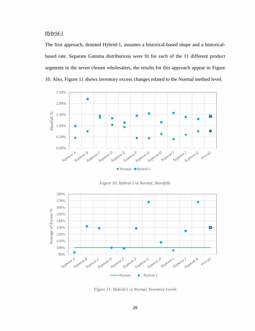
Hybrid-1

The first approach, denoted Hybrid-1, assumes a historical-based shape and a historical-

based rate. Separate Gamma distributions were fit for each of the 11 different product

segments in the seven chosen wholesalers, the results for this approach appear in Figure

10. Also, Figure 11 shows inventory excess changes related to the Normal method level.

Figure 10: Hybrid-1 vs Normal, Shortfalls

Figure 11: Hybrid-1 vs Normal, Inventory Levels

0.00%

0.50%

1.00%

1.50%

2.00%

2.50%

Sho

rtfa

ll %

Normal Hybrid-1

90%

100%

110%

120%

130%

140%

150%

160%

170%

180%

Aver

age

of

Exce

ss %

Normal Hybrid-1

27

Observe that approach Hybrid-1 performs quite poorly. In every segment, Hybrid-1 has a

greater percentage of shortfalls than does the Normal method. In fact, Hybrid-1 is

dominated by the Normal method for many segments, such as segment B, for which

Hybrid-1 has a greater shortfall percentage and also an increased inventory level. This poor

performance is likely due to the fact that the demand levels are not stationary over time,

but instead are forecast to vary significantly over time, due to seasonal effects.

Hybrid-2

The second approach, denoted Hybrid-2 assumes a forecast-based shape and a forecast-

based rate. Separate distributions were again fit for each of the 11 product segments in

these seven wholesalers, the results of this strategy are presented in Figure 12.


Figure 13 reveals how much excess inventory increases under the Hybrid-2 approach with

respect to the Normal method.

0.00%

0.20%

0.40%

0.60%

0.80%

1.00%

1.20%

1.40%

1.60%

Sho

rtfa

ll %

Normal Hybrid-2

28


The company’s goal is a 99.78% service level which implies stock-outs no more than

0.22% of the time. Hybrid-2 method shows better performance in comparison to the

traditional Normal method. By this method, the shortfall percentage decreased for every

segment, and the service level of four segments are at a value less than or equal to the target

level of 0.22%. Moreover, these stock-outs reductions were achieved without imposing

large increases to the current inventory level, with the average excess inventory only

increased by 40%.

Hybrid-3

The third method uses a Gamma distribution is denoted Hybrid-3, this approach utilizes a

historical-based shape parameter and a forecast-based rate parameter. Separate Gamma

distributions were fit for each of the 11 different product segments in these seven

wholesalers, the results for this approach appear in Figure 14. Figure 15 reveals how much

excess inventory increases under the Hybrid-3 approach in comparison with the Normal

method.

90%

100%

110%

120%

130%

140%

150%

160%

170%

180%

190%

Aver

age

of

Exce

ss %

Normal Hybrid-2

29



The results for the Hybrid-3 approach are somewhat mixed. For 6 of the 11 segments,

Hybrid-3 generates fewer stock-outs than does the Normal method, another segment has

equal performance across the two methods. However, for every segment considered,

Hybrid-3 generates increased excess inventory, although these increases are in many cases

not terribly large: only 3 segments show an increase in excess inventory of greater than

25% under the Hybrid-3 approach for inventory requirements.

0.00%

0.50%

1.00%

1.50%

2.00%

2.50%

3.00%

Sho

rtfa

ll %

Normal Hybrid-3

90%

100%

110%

120%

130%

140%

150%

Aver

age

of

Exce

ss %

Normal Hybrid-3

30

Hybrid-4

The final method examined, denoted Hybrid-4, uses a Gamma distribution with a forecast-

based shape parameter and a historical-based rate parameter. Separate Gamma distributions

were again fit for each of the 11 different product segments in these seven wholesalers, the

results for this approach appear in Figure 16.


Figure 17 reveals how much excess inventory increases under the Hybrid-4 approach

with respect to the Normal method.


0.00%

0.20%

0.40%

0.60%

0.80%

1.00%

1.20%

1.40%

1.60%

Sho

rtfa

ll %

Normal Hybrid-4

90%

140%

190%

240%

290%

340%

390%

440%

490%

540%

Aver

age

of

Exce

ss %

Normal Hybrid-4

31

Examining the performance of Hybrid-4, we observe that it generates very infrequent

stock-outs, in fact, for 8 of the 11 segments, the shortfall rate is less than the target of

0.22%. However, these reductions in shortfalls are accomplished via an extremely large

increase in average excess inventory, with every segment but one increasing the average

excess inventory by more than 100%, relative to the Normal method.

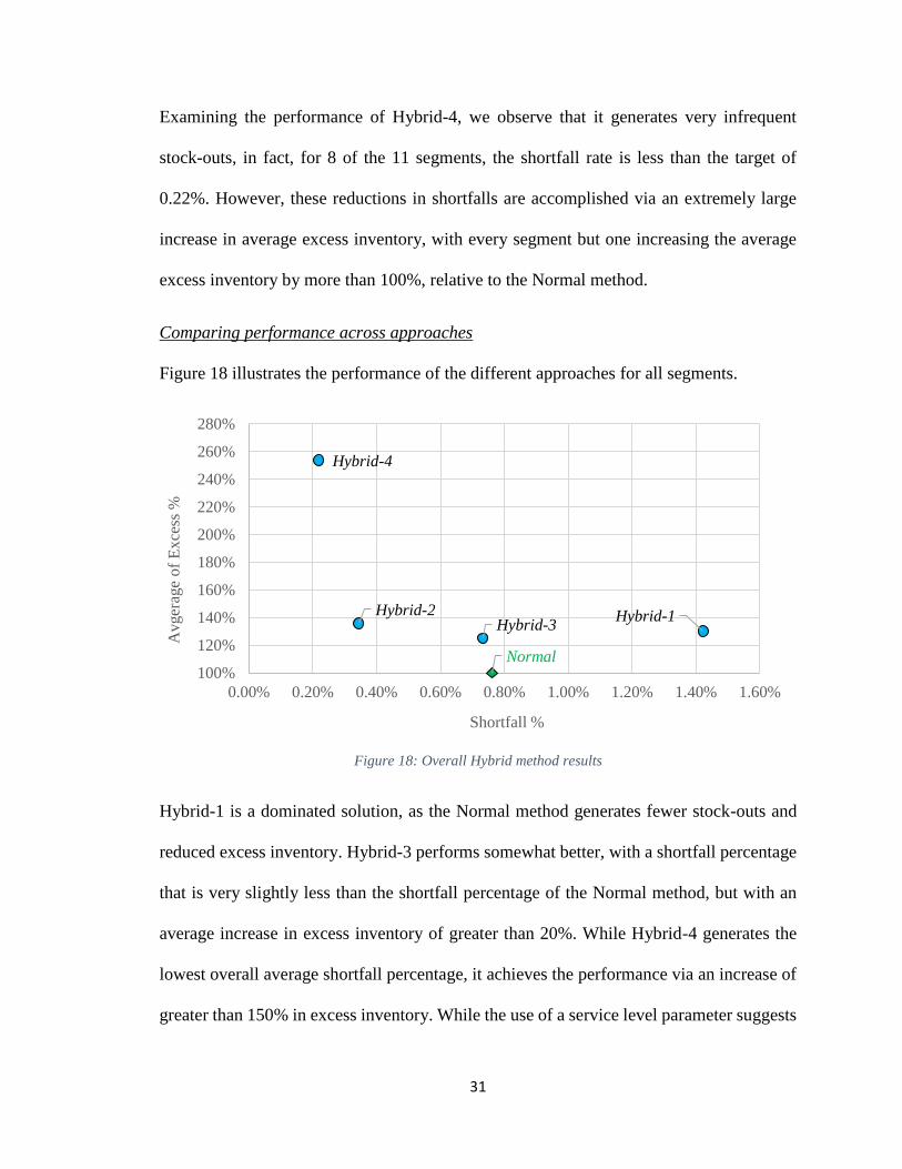
Comparing performance across approaches

Figure 18 illustrates the performance of the different approaches for all segments.

Figure 18: Overall Hybrid method results

Hybrid-1 is a dominated solution, as the Normal method generates fewer stock-outs and

reduced excess inventory. Hybrid-3 performs somewhat better, with a shortfall percentage

that is very slightly less than the shortfall percentage of the Normal method, but with an

average increase in excess inventory of greater than 20%. While Hybrid-4 generates the

lowest overall average shortfall percentage, it achieves the performance via an increase of

greater than 150% in excess inventory. While the use of a service level parameter suggests

Normal

Hybrid-1Hybrid-2Hybrid-3

Hybrid-4

100%

120%

140%

160%

180%

200%

220%

240%

260%

280%

0.00% 0.20% 0.40% 0.60% 0.80% 1.00% 1.20% 1.40% 1.60%

Avger

age

of

Exce

ss %

Shortfall %

32

that shortfalls are viewed as much more troubling than inventory holding costs, an increase

of this magnitude is so large as to suggest that approach Hybrid-4 is likely infeasible, due

to storage space limitations at the wholesalers. Approach Hybrid-2, which utilizes forecast-

based values for both the assumed Gamma distribution's shape and rate parameters, is

arguably the best-performing approach for this test case data set. It achieves an overall

average shortfall rate of 0.38%, while only increasing the average excess inventory by

37%, relative to the baseline Normal approach.

33

Chapter 4: Conclusions and Further Study

Conclusions and Further Study

4-1 Conclusions

In this work, we offered an alternative solution for safety stock and inventory level

problems. The traditional methodology assumes that demand during lead time follows a

normal distribution. A case study, based on data from a liquid consumer packaged goods

company, was used to evaluate alternative techniques for setting the target inventory levels.

In the first alternative approach studied, referred to as the service level adjustment method,

the Z-value associated with the normal distribution was increased until the observed

performance in the data set achieved the desired service level of 0.22% stock-outs. This

required use of a Z-value equal to 4.3, which, according to the theoretical normal

distribution, should generate 0.0009% stock-outs. A drawback to this approach is that it

requires extensive computational testing, evaluating the performance of alternative Z-

values until one is encountered that achieves the desired service level in the test data set.

Such an approach could be very difficult to implement in a situation with a large number

of items and suppliers.

A hybrid approach, utilizing the Gamma probability density function, was examined next.

A variety of historical-based and forecasted-based combinations was utilized to fit the

Gamma distribution's shape and rate parameters. The Hybrid-2 approach, which utilized a

forecast-based approach for estimating both the Gamma distribution shape and rate

parameters, was observed to perform best for our test case example.

34

Table 6 shows the results related to the three selected approaches across all wholesalers.

As presented in Table 6, the Hybrid-2 approach is able to generate a shortfall rate that is

half the value of the Normal method, with a 37% average increase in excess inventory. The

service level adjustment technique finds that the shortfall can be reduced to the target level

of 0.22%, but only by accepting an average increase of 49% in excess inventory. Since the

service level adjustment technique cannot be easily adopted for use in general settings with

many segments and data points, we view Hybrid-2, which is a non-dominated solution, as

the preferred method, since it can easily and quickly be implemented for large data sets

with many product segments.

Table 2: Comparing all methods across all wholesalers

Normal Normal:

Service level adjustment Hybrid-2

Shortfall Avg.

Excess Shortfall Avg. Excess Shortfall

Avg.

Excess

Among All

Records 0.75% ℬ 0.22% 1.49ℬ 0.38% 1.37ℬ

In other words, we can use the Gamma distribution with forecast-based parameters to find

inventory levels for problems whose demand during lead time distributions have long tail

distributions and find solutions that outperform the Normal approach.

4-2 Further study

The current study mainly focuses on Gamma and Normal distributions, therefore the

offered approaches are limited to these two distributions. It is possible that by choosing

different distributions the results could be improved. Furthermore, quantile forecasting

method (Ghodsypour and O’brien 2001) could be another alternative method for finding

35

safety stock levels in such situations, since quantile regression estimates are often more

robust against outliers in the response measurements than the Normal method.

36

References

Alp, O., N.K. Erkip, and R. Güllü. 2003. Optimal lot-sizing/vehicle-dispatching policies

under stochastic lead times and stepwise fixed costs. Operations Research

51(1):160-166.

Ben-Daya, M., and A. Raouf. 1994. Inventory models involving lead time as a decision

variable. Journal of the Operational Research Society 45(5):579-582.

Bourland, K.E., and C.A. Yano. 1994. The strategic use of capacity slack in the economic

lot scheduling problem with random demand. Management Science 40(12):1690-

1704.

Braglia, M., D. Castellano, and M. Frosolini. 2016. A novel approach to safety stock

management in a coordinated supply chain with controllable lead time using present

value. Applied Stochastic Models in Business and Industry 32(1):99-112.

Brander, P., and R. Forsberg. 2006. Determination of safety stocks for cyclic schedules

with stochastic demands. International Journal of Production Economics

104(2):271-295.

Chaturvedi, A., and V. Martínez‐de‐Albéniz. 2016. Safety Stock, Excess Capacity or

Diversification: Trade‐Offs under Supply and Demand Uncertainty. Production

and Operations Management 25(1):77-95.

Chopra, S., G. Reinhardt, and M. Dada. 2004. The effect of lead time uncertainty on safety

stocks. Decision Sciences 35(1):1-24.

Doll, C.L., and D.C. Whybark. 1973. An iterative procedure for the single-machine multi-

product lot scheduling problem. Management Science 20(1):50-55.

37

Federgruen, A., and Z. Katalan. 1996. The stochastic economic lot scheduling problem:

cyclical base-stock policies with idle times. Management Science 42(6):783-796.

Fortuin, L. 1980. Five popular probability density functions: A comparison in the field of

stock-control models. Journal of the Operational Research Society 31(10):937-

942.

Gallego, G. 1990. Scheduling the production of several items with random demands in a

single facility. Management Science 36(12):1579-1592.

Ghodsypour, S.H., and C. O’brien. 2001. The total cost of logistics in supplier selection,

under conditions of multiple sourcing, multiple criteria and capacity constraint.

International journal of production economics 73(1):15-27.

Inderfurth, K., and S. Vogelgesang. 2013. Concepts for safety stock determination under

stochastic demand and different types of random production yield. European

Journal of Operational Research 224(2):293-301.

Kelle, P., G. Clendenen, and P. Dardeau. 1994. Economic lot scheduling heuristic for

random demands. International Journal of Production Economics 35(1-3):337-

342.

Liao, C.-J., and C.-H. Shyu. 1991. An analytical determination of lead time with normal

demand. International Journal of Operations & Production Management 11(9):72-

78.

Madadi, A., M.E. Kurz, and J. Ashayeri. 2010. Multi-level inventory management

decisions with transportation cost consideration. Transportation Research Part E:

Logistics and Transportation Review 46(5):719-734.

38

Moncayo-Martínez, L.A., and D.Z. Zhang. 2013. Optimising safety stock placement and

lead time in an assembly supply chain using bi-objective MAX–MIN ant system.

International Journal of Production Economics 145(1):18-28.

Ouyang, L.-Y., N.-C. Yeh, and K.-S. Wu. 1996. Mixture inventory model with backorders

and lost sales for variable lead time. Journal of the Operational Research Society

47(6):829-832.

Ross, S. 1983. Stochastic Processes. Series in Probability and Mathematical Statistics.

Wiley, New York.

Silver, E.A., D.F. Pyke, and R. Peterson. 1998. Inventory management and production

planning and scheduling. Wiley New York.

Smits, S.R., M. Wagner, and T.G. de Kok. 2004. Determination of an order-up-to policy

in the stochastic economic lot scheduling model. International Journal of

Production Economics 90(3):377-389.

Snyder, R. 1984. Inventory control with the gamma probability distribution. European

Journal of Operational Research 17(3):373-381.

Sox, C.R., P.L. Jackson, A. Bowman, and J.A. Muckstadt. 1999. A review of the stochastic

lot scheduling problem. International Journal of Production Economics 62(3):181-

200.

Tersine, R.J. 1994. Principles of inventory and materials management.

Tyworth, J.E., and A.Z. Zeng. 1998. Estimating the effects of carrier transit-time

performance on logistics cost and service. Transportation Research Part A: Policy

and Practice 32(2):89-97.

39

Yang, M.-F. 2010. Supply chain integrated inventory model with present value and

dependent crashing cost is polynomial. Mathematical and Computer Modelling

51(5):802-809.

Documents

ALTERNATIVE METHODS FOR CALCULATING OPTIMAL SAFETY …