Alternatives to Cap-Weighted Indices - EDHEC …docs.edhec-risk.com/nwl/110131/Alternatives_to_Cap...Alternatives to Cap-Weighted Indices EDHEC Institutional Days Monaco, December

Alternatives to Cap-Weighted Indices

EDHEC Institutional DaysMonaco, December 8th, 2010, 14:15-15:30

2

Lionel Martellini

Professor of Finance, EDHEC Business SchoolScientific Director, EDHEC Risk Institute

[email protected]

3

Introduction: Beyond Cap-Weighting

In Search of Representative Indices– Cap-Weighting– Fundamental Weights

Designing Efficient Investment Benchmarks– Ad-Hoc Diversification: De-concentrating Portfolios– Scientific Diversification: Towards the Efficient Frontier

Alternative Weighting Schemes: Conditions for Optimality?

Conclusion: Concept Selection vs. Concept Diversification

Outline

4






5

A number of (index or fund) providers have recently designed and launched non cap-weighted indices.

The (non-exhaustive) list includes: – fundamental indices– equally-weighted indices– minimum variance indices– efficient indices– equal-risk contribution (a.k.a. risk parity) indices– maximum diversification indices

This presentation provides a summary of the objectives of, and assumptions behind, the various indexing concepts.

Beyond Cap WeightingComparing Alternatives

6

Beyond Cap WeightingConcepts versus Figures

We will not focus so much on past performance; track records (bydefinition) all look pretty good!

Instead, we propose to provide an academic perspective on the conceptual assumptions underpinning the different methods.– (Even out-of-sample) track records are sample-dependent and thus

performance figures rely on the data and time period at hand. – For long-term benchmarks, it is important that performance is driven

by a sound concept that relies on reasonable assumptions rather than by exploiting anomalies in past returns data.

– If achieving higher risk-adjusted performance is not the focus of a methodology, achieving it is at best a collateral benefit.

In Seneca’s words (circa 30 BC):“If one does not know to which port one is sailing, no wind is favorable.”

7

The words « index » and « benchmark » are often used interchangeably; yet they define a priori very different concepts.

Market perspective: an index is a portfolio that should represent the performance of a given segment of the market. => focus on representativity

Investor perspective: a benchmark is a reference portfolio that should represent the fair reward expected in exchange for risk exposures that an investor is willing to accept. => focus on efficiency

CW portfolios have long been portrayed as representative and efficient, but have faced increased criticism on both fronts.

Beyond Cap-WeightingWhich Port do we want to Sail to: Indices versus Benchmarks

8






9

A market cap weighted scheme is the obvious default option when it comes to representing a given segment of the market.– Market cap weighted indices provide by construction a fair

representation of the stock market;– In the end, cap-weighting is nothing but an ad-hoc weighting

scheme that achieves some form of representativity.

Cap-weighted indices, however, may not provide a fair representation of the underlying economic fundamentals.

Some have argued that they represent well the stock market but not the economy.

In Search of Representative IndicesCap-Weighting for Representativity?

10

Rather than using the market cap, fundamental indices use firm attributes such as book value, dividends, sales or cash flows as measures of size.

These indices aim at better representing the economy.Arnott (2007): “The Fundamental Index weights companies in

accordance to their footprint in the broad economy […] you wind up with a portfolio that mirrors the economy”.

Whether or not fundamentally weighted indices better represent the economy is actually an open question, if only because representativity is not a concept that is linked to clear measures.

In Search of Representative IndicesFundamental Weighting for Representativity?

11






12

In any case, it is not clear why investors would care about their portfolios representing the economy.

From the investor’s perspective, the focus should be on efficiency: obtaining fair rewards for given risk budgets.

Efficiency is intimately related to diversification: it is by constructing well-diversified portfolios that one can achieve a fair reward for a given risk exposure.

CW portfolios in fact appear to be rather inefficient and poorlydiversified portfolios, and several approaches have been developed so as to improve diversification compared to cap-weighting.

Designing Efficient Investment BenchmarksEfficiency is Related to Diversification

13

Cap-weighting is often believed to lead to risk/reward efficient portfolios, but that belief is not really based on firm grounds.

The belief in efficiency of CW is based on a naïve interpretation of W. Sharpe’s Capital Asset Pricing Model (CAPM):– No need to gather any information on risk & return parameters

to find optimal portfolios ... because everybody else does!– When relaxing the highly unrealistic assumptions of the CAPM,

financial theory does not predict that the market portfolio is efficient (Sharpe (1991), Markowitz (2005)).

– If there are multiple risk factors, the mean-variance optimal portfolio is no longer CW (Merton (1971), Cochrane (1999)); in a post-CAPM multi-factor world, CW is just an arbitrary weighting scheme.

Designing Efficient Investment Benchmarks Cap-Weighting for Efficiency?

14

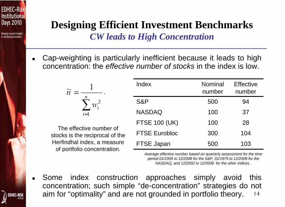
Cap-weighting is particularly inefficient because it leads to high concentration: the effective number of stocks in the index is low.

Some index construction approaches simply avoid this concentration; such simple “de-concentration” strategies do not aim for “optimality” and are not grounded in portfolio theory.

The effective number of stocks is the reciprocal of the Herfindhal index, a measure

of portfolio concentration.

Index Nominal number

Effective number

S&P 500 94

NASDAQ 100 37

FTSE 100 (UK) 100 28

FTSE Eurobloc 300 104

FTSE Japan 500 103Average effective number based on quarterly assessment for the time

period 01/1959 to 12/2008 for the S&P, 01/1975 to 12/2008 for the NASDAQ, and 12/2002 to 12/2008 for the other indices .

Designing Efficient Investment Benchmarks CW leads to High Concentration

15






Naïve de-concentration: – Equal-weighting simply gives the same weight to each of N stocks

in the index (“1/N rule”).– Equal-weighting is the naïve route to constructing well diversified

portfolios.

Semi-naïve de-concentration:– Equal risk contribution (ERC) takes into account contribution to risk.– Contribution to risk is not proportional to dollar contribution.– Find portfolio weights such that contributions to risk are equal

(Maillard, Roncalli and Teiletche (2010)):

Ad-Hoc Approach to Well-Diversified PortfoliosEqual Weighting and Equal Risk Contribution

16 16

j

pj

i

pi w

ww

w∂

∂=

∂

∂ σσ

Statistical de-concentration:– Define a diversification index and try and maximize it by utilizing the

correlations that drive the magic of diversification: “The whole is better than the sum of its parts”.

– Maximum Diversification (also known as anti-benchmark) aims at generating portfolios with the highest possible diversification index (Choueifaty and Coignard (2008)):

The weighted average risk (in the numerator) will be high compared to portfolio risk (in the denominator) and thus DI will be high if the

portfolio weights exploit well the correlations.

Ad-Hoc Approach to Well-Diversified Portfolios Maximum Diversification Benchmarks/Anti-Benchmark

⎟⎟⎟⎟⎟⎟

⎠

⎞

⎜⎜⎜⎜⎜⎜

⎝

⎛

=

∑

∑

=

=n

jiijji

n

iii

www

wMaxDI

1,

1

σ

σ

17

18






Scientific Approach to Well-Diversified PortfoliosTowards the Efficient Frontier

19 19

Scientific diversification is based on reaching a high risk/return objective through portfolio construction techniques.

In practice, to get a decent proxy for efficient portfolios, one needs to use careful risk and return parameter estimates; practical approaches to scientific diversification make different choices regarding the challenge of risk and return estimation.

Technology is available to generate reliable risk parameter estimates:– Suitably designed factor models to mitigate the curse of

dimensionality (see also statistical shrinkage techniques).– Accounting for non-stationarity: e.g., GARCH and Regime Switching

models.

On the other hand, statistics is close to useless in terms of expected return estimation (Merton (1980)).

Volatility

ExpectedReturn

Maximum Sharpe Ratio (MSR) Portfolio

●

Scientific Approach to Well-Diversified PortfoliosGMV vs. MSR

Global Minimum Variance

(GMV)Portfolio

●

The MSR provides the highest reward per unit of portfolio volatility: needed optimization inputs are expected returns, correlations and volatilities.The GMV provides the lowest possible portfolio volatility: needed optimization inputs are correlations and volatilities. 20

If you feel comfortable about estimating risk parameters the variance-covariance matrix, but not about estimating expected return parameters, the global minimum variance (GMV) benchmark is the way to go (e.g., Amenc and Martellini (2003)).

Scientific Approach to Well-Diversified PortfoliosMinimum Variance Benchmarks (GMV)

21

This approach provides a low volatility portfolio but also a low performance portfolio: ex-ante, MSR+cash is better than GMV.

Ex-post, MV portfolios tend to beconcentrated portfolios with overweighting of low volatility stocks, with a Sharpe ratio lowerthan that of EW (Garlappi et al. (2007)).

21

0 5 10 15 20 250

2

4

6

8

10

12

14

16

18

Ann

ualiz

ed e

xpec

ted

retu

rn

Annualized volatility

Efficient frontierTangency line

GMV

MSR

MSR + cash

22

Scientific Approach to Well-Diversified PortfoliosEfficient Indexation (MSR)

Efficient Indexation is about maximizing the Sharpe ratio.

Just like in the Minimum Variance approach, Efficient Indexation exploits information on the covariance matrix of stock returns; the approach uses suitably designed factor models to mitigate the curse of dimensionality.

While direct estimation of expected returns from past returns isuseless, all hope on expected returns estimation is not lost!

Common sense suggests that expected return parameters should be positively related to risk parameters (risk-return tradeoff ).

Efficient Indexation uses indirect estimation of expected returns through a stock’s riskiness.

23

Theory unambiguously confirms the existence of a positive risk/return relationship:– Systematic risk is rewarded (APT);– Specific risk is also rewarded (Merton (1987)) (*);– Total volatility (model-free) should therefore be rewarded;– Higher moment risk is also rewarded (many references).

Use the risk-return relationship to build efficient portfolios: magic of diversification is about mixing high-risk-and-therefore-high-return stocks in a smart way so as to generate low risk portfolios!

(*) See also Barberis and Huang (2001) Malkiel and Yu (2002), Boyle, Garlappi, Uppal and Wang (2009) .

Scientific Approach to Well-Diversified Portfolios On the Risk-Return Relationship

Scientific Approach to Well-Diversified Portfolios iv Puzzle – VW Portfolios over Short Horizons

•Ang, Hodrick, Xing and Zhang (2006, 2009): “iv puzzle”•12 Month idiosyncratic volatility •1 Month realized return•10 VW Portfolios•Value Weighted Portfolio returns•Negative Relationship•High-Low returns mainly driven by high iVol portfolio

Value Weighted Portfolios: Short Horizon (iVol)

0.00

0.01

0.10

1.00

10.00

100.00

1000.00

64' 67' 70' 73' 76' 79' 82' 85' 88' 91' 94' 97' 00' 03' 06' 09'

Valu

e of

1$

inve

sted

in 1

964

Low 2 3 4 5 6 7 8 9 High

Value Weighted Portfolios: Short Horizon (iVol)

-10.0%

-5.0%

0.0%

5.0%

10.0%

15.0%

20.0%

25.0%

0% 5% 10% 15% 20% 25% 30%

Average Risk over Cross-Section

Ave

rage

Por

tfol

io R

etur

n an

d St

anda

rd E

rror

Bou

nds

Ten VW portfolios containing an equal number of stocks (extracted from the CRSP data base) are built every month after sorting the stocks based on some risk measure, here idiosyncratic volatility w.r.t. FF

model (calculated using daily data for last 12 months); the returns of each of these portfolios are

calculated subsequent one-month periods and averaged across the portfolio formation date.

Scientific Approach to Well-Diversified Portfolios No iv Puzzle – EW Portfolios over Short Horizons

•Negative relationship disappears when EW used.•Extremely low return of High-Volatility portfolio disappears.•We still do not have a positive relationship.

• Return reversal : Huang, Liu, Rhee, and Zhang (2009)• Extreme winners and losers (over the past month)typically have high iVol over the last 1 month• In high iVol portfolios: # past winners is almost equal to # past losers, but average weight of past winners issubstantially larger.• Short-term return reversal effect: past-month winnerstend to under perform in subsequent month .• So, VW lowers the portfolio return compared to otherportfolios and EW does not.

Equally Weighted Portfolios: Short Horizon (iVol)

0.10

1.00

10.00

100.00

1000.00

10000.00

64' 67' 70' 73' 76' 79' 82' 85' 88' 91' 94' 97' 00' 03' 06' 09'Valu

e of

1$

inve

sted

in 1

964

Low 2 3 4 5 6 7 8 9 High

Equally Weighted Portfolios: Short Horizon (iVol)

-10.0%

-5.0%

0.0%

5.0%

10.0%

15.0%

20.0%

25.0%

0% 5% 10% 15% 20% 25% 30%


Ave

rage

Por

tfol

io R

etur

n an

d St

anda

rd E

rror

Bou

nds

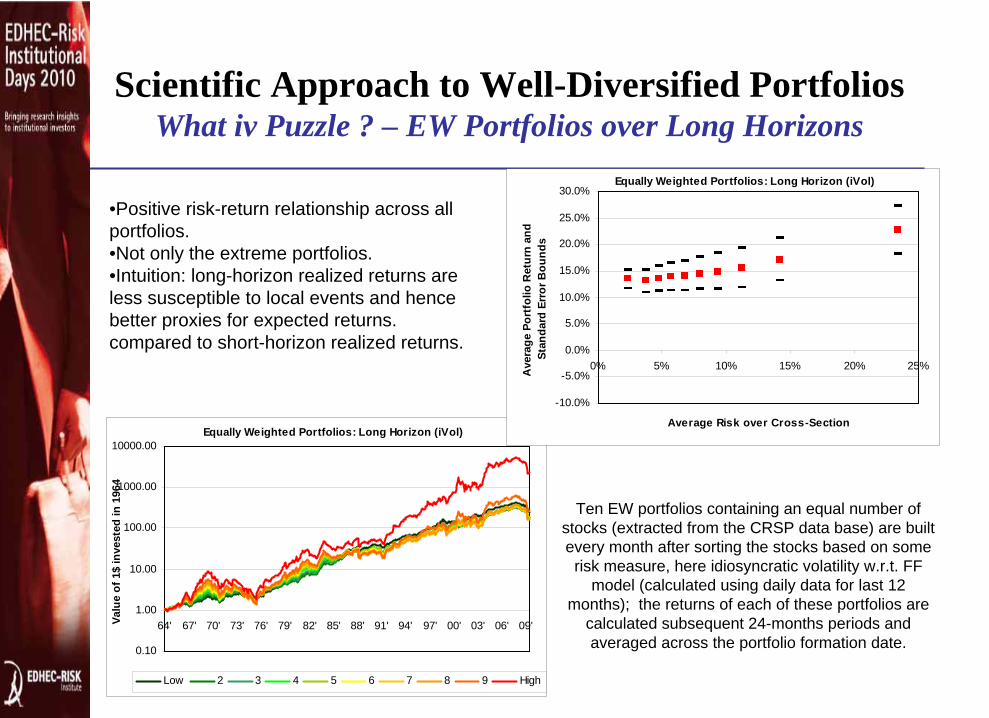
•Positive risk-return relationship across all portfolios.•Not only the extreme portfolios.•Intuition: long-horizon realized returns are less susceptible to local events and hence better proxies for expected returns. compared to short-horizon realized returns.

Equally Weighted Portfolios: Long Horizon (iVol)

0.10

1.00

10.00

100.00

1000.00

10000.00

64' 67' 70' 73' 76' 79' 82' 85' 88' 91' 94' 97' 00' 03' 06' 09'Valu

e of

1$

inve

sted

in 1

964

Low 2 3 4 5 6 7 8 9 High

Equally Weighted Portfolios: Long Horizon (iVol)

-10.0%

-5.0%

0.0%

5.0%

10.0%

15.0%

20.0%

25.0%

30.0%

0% 5% 10% 15% 20% 25%


Ave

rage

Por

tfol

io R

etur

n an

d St

anda

rd E

rror

Bou

nds

Scientific Approach to Well-Diversified Portfolios What iv Puzzle ? – EW Portfolios over Long Horizons

Ten EW portfolios containing an equal number of stocks (extracted from the CRSP data base) are built every month after sorting the stocks based on some risk measure, here idiosyncratic volatility w.r.t. FF

model (calculated using daily data for last 12 months); the returns of each of these portfolios are

calculated subsequent 24-months periods and averaged across the portfolio formation date.

• Blitz and Vliet (2007) •12 Month total volatility •1 Month realized return•10 Portfolios•Value Weighted Portfolio returns•Negative risk-return relationship• High-Low returns mainly driven by low tVol portfolio

Value Weighted Portfolios: Short Horizon (tVol)

0.01

0.10

1.00

10.00

100.00

1000.00

64' 67' 70' 73' 76' 79' 82' 85' 88' 91' 94' 97' 00' 03' 06' 09'

Valu

e of

1$

inve

sted

in 1

964

Low 2 3 4 5 6 7 8 9 High

Value Weighted Portfolios: Short Horizon (tVol)

-10.0%

-5.0%

0.0%

5.0%

10.0%

15.0%

20.0%

25.0%

0% 5% 10% 15% 20% 25% 30%


Ave

rage

Por

tfol

io R

etur

n an

d St

anda

rd E

rror

Bou

nds

Scientific Approach to Well-Diversified Portfoliostv Puzzle – VW Portfolios over Short Horizons

Ten VW portfolios containing an equal number of stocks (extracted from the CRSP data base) are built every month after sorting the stocks based on some risk measure, here total volatility (calculated using

daily data for last 12 months); the returns of each of these portfolios are calculated subsequent one-month periods and averaged across the portfolio

formation date.

•12 Month total volatility •1 Month realized return•10 Portfolios•Equally Weighted Portfolio returns

•Again, Negative relationship disappears when EW used.• Extremely low return of High-Volatility portfolio disappears.•We still do not have a positive relationship.

Equally Weighted Portfolios: Short Horizon (tVol)

0.10

1.00

10.00

100.00

1000.00

64' 67' 70' 73' 76' 79' 82' 85' 88' 91' 94' 97' 00' 03' 06' 09'Valu

e of

1$

inve

sted

in 1

964

Low 2 3 4 5 6 7 8 9 High

Equally Weighted Portfolios: Short Horizon (tVol)

-10.0%

-5.0%

0.0%

5.0%

10.0%

15.0%

20.0%

25.0%

0% 5% 10% 15% 20% 25% 30%


Ave

rage

Por

tfol

io R

etur

n an

d St

anda

rd E

rror

Bou

nds

Scientific Approach to Well-Diversified PortfoliosNo tv Puzzle – EW Portfolios over Short Horizons

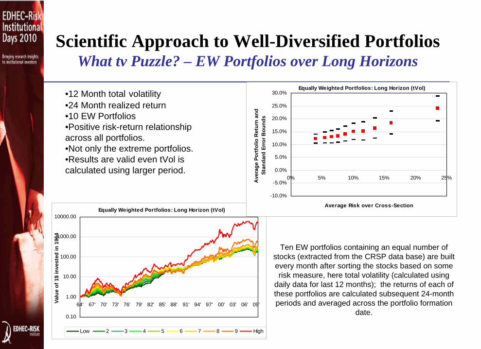
•12 Month total volatility •24 Month realized return•10 EW Portfolios•Positive risk-return relationship across all portfolios.•Not only the extreme portfolios.•Results are valid even tVol is calculated using larger period.

Equally Weighted Portfolios: Long Horizon (tVol)

0.10

1.00

10.00

100.00

1000.00

10000.00

64' 67' 70' 73' 76' 79' 82' 85' 88' 91' 94' 97' 00' 03' 06' 09'Valu

e of

1$

inve

sted

in 1

964

Low 2 3 4 5 6 7 8 9 High

Equally Weighted Portfolios: Long Horizon (tVol)

-10.0%

-5.0%

0.0%

5.0%

10.0%

15.0%

20.0%

25.0%

30.0%

0% 5% 10% 15% 20% 25%


Ave

rage

Por

tfol

io R

etur

n an

d St

anda

rd E

rror

Bou

nds

Scientific Approach to Well-Diversified Portfolios What tv Puzzle? – EW Portfolios over Long Horizons

Ten EW portfolios containing an equal number of stocks (extracted from the CRSP data base) are built every month after sorting the stocks based on some risk measure, here total volatility (calculated using

daily data for last 12 months); the returns of each of these portfolios are calculated subsequent 24-month periods and averaged across the portfolio formation

date.

Evidence that stock downside risk is related to expected returns

Scientific Approach to Well-Diversified Portfolios Downside Risk & Expected Returns

Authors Risk Measure MomentsZhang (2005) Skewness SkewBoyer, Mitton and Vorkink (2009)

Skewness Skew

Tang and Shum (2003) Skewness Skew

Connrad, Dittmar and Ghysels (2009)

Skewness Skew

Ang et al. (2006) Downside correlation Vol, Skew, KurtHuang et al (2009) Value-at-Risk (EVT) Vol, Skew, KurtBali and Cakici (2004) Value-at-Risk

(Historical)Vol,Skew, Kurt

Chen et al. (2009) Semi-deviation Vol, Skew, KurtEstrada (2000) Semi-deviation Vol, Skew, Kurt

Scientific Approach to Well-Diversified Portfolios Total Semi-Deviation – EW Decile Portfolios Long Horizon

•12 Month Total Semi-Deviation•24 Month realized return•10 Portfolios•Equally Weighted Portfolio returns

Equally Weighted Portfolios: Long Horizon (semi-deviation)

1.00

10.00

100.00

1000.00

10000.00

64' 67' 70' 73' 76' 79' 82' 85' 88' 91' 94' 97' 00' 03' 06' 09'

Valu

e of

1$

inve

sted

in 1

964

Low 2 3 4 5 6 7 8 9 High

Equally Weighted Portfolios: Long Horizon (semi-deviation)

-10.0%

-5.0%

0.0%

5.0%

10.0%

15.0%

20.0%

25.0%

30.0%

0% 5% 10% 15% 20%


Ave

rage

Por

tfol

io R

etur

n an

d St

anda

rd E

rror

Bou

nds

•Positive risk-return relationship across all portfolios.•Not only the extreme portfolios.•Results are valid even semi-deviation is calculated using larger period.

32

The average cumulative return for portfolios sorted on semi-deviation.

0%

10%

20%

30%

40%

50%

60%

70%

80%

1 2 3 4 5 6 7 8 9 10 11 12 13 14 15 16 17 18 19 20 21 22 23 24 25 26 27 28 29 30 31 32 33 34 35 36

Month after portfolio formation

Port Low

Port 2

Port 3

Port 4

Port 5

Port 6

Port 7

Port 8

Port 9

Port High

Ten portfolios containing an equal number of stocks (extracted from the CRSP data base) are built every month after sorting the stocks based on their semi-deviation (calculated using daily data for last 30 months); the cumulative returns of each of these portfolios are

calculated for various holding periods and averaged across the portfolio formation date.

Scientific Approach to Well-Diversified Portfolios Downside Risk and Expected Returns

Scientific Approach to Well-Diversified Portfolios Long-Term Results

IndexAnn.

average return

Ann. std.Deviation

Sharpe Ratio

Information Ratio

TrackingError

Efficient Index 11.63% 14.65% 0.41 0.52 4.65%Cap-weighted 9.23% 15.20% 0.24 0.00 0.00%Difference (Efficient minus Cap-weighted) 2.40% -0.55% 0.17 - -

p-value for difference 0.14% 6.04% 0.04% - -

The table shows risk and return statistics portfolios constructed with using the same set of constituents as the cap-weighted S&P 500 index. Rebalancing is quarterly subject to an optimal control of portfolio turnover (by setting the reoptimisation threshold to 50%). Portfolios are

constructed by maximising the Sharpe ratio given an expected return estimate and a covariance estimate. The expected return estimate is set to the median total risk of stocks in the same decile when sorting on total risk. The covariance matrix is estimated using an implicit factor

model for stock returns. Weight constraints are set so that each stock's weight is between 1/2N and 2/N, where N is the number of index constituents. P-values for differences are computed using the paired t-test for the average, the F-test for volatility, and a Jobson-Korkie test for the Sharpe ratio. The results are based on weekly return data from 01/1959. We use a calibration period of 2 years and rebalance the

portfolio every three months (at the beginning of January, April, July and October).

33

34






Each of the aforementioned weighting methods makes different methodological choices.

However, portfolio theory tells us that there is only one optimal portfolio: the tangency (MSR) portfolio.

Question: Under which conditions would the portfolio construction choices of different index weighting schemes be truly optimal?

KIS(BNTS) principle: robustness of a method may justify simple assumptions but is important that assumptions also remain reasonable; if the conditions are too restrictive, we are unlikely to obtain optimal portfolios.

35

Conditions for OptimalityKeep it Simple… But Not Too Simple

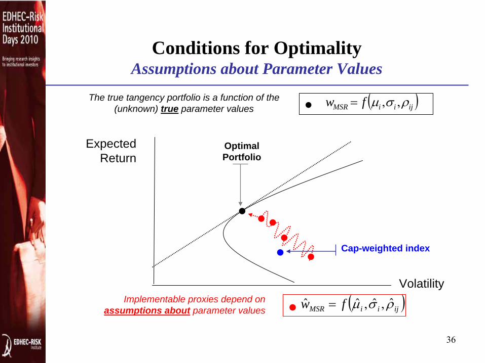
Volatility

ExpectedReturn

The true tangency portfolio is a function of the (unknown) true parameter values

OptimalPortfolio

( )ijiiMSR fw ρσμ ,,=

Implementable proxies depend on assumptions about parameter values

●

●●

●●

( )ijiiMSR fw ρσμ ˆ,ˆ,ˆˆ =●

●

● Cap-weighted index

36

Conditions for OptimalityAssumptions about Parameter Values

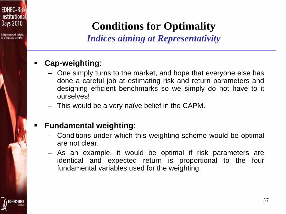
Conditions for OptimalityIndices aiming at Representativity

Cap-weighting: – One simply turns to the market, and hope that everyone else has

done a careful job at estimating risk and return parameters and designing efficient benchmarks so we simply do not have to it ourselves!

– This would be a very naïve belief in the CAPM.

Fundamental weighting: – Conditions under which this weighting scheme would be optimal

are not clear.– As an example, it would be optimal if risk parameters are

identical and expected return is proportional to the four fundamental variables used for the weighting.

37

Conditions for OptimalityDe-Concentration Approaches

Equal-weighting: – Optimal if and only if one assumes all stocks have the same

expected return and…– … the same volatility and…– … the same pairwise correlations!

Equal Risk Contribution (Maillard et al. (2010)):– Optimal if and only if one assumes all stocks have same

Sharpe ratios and…– … the same pairwise correlations.

Maximum Diversification (Choueifaty and Coignard (2008)):– Optimal if and only if one assumes all stocks have same

Sharpe ratios.38

Conditions for OptimalityEfficient Frontier Approaches

Minimum Variance:– Only optimal if one assumes that all stocks have the same

expected returns, hardly a neutral/reasonable choice.

Efficient Indexation:– Optimal if one assumes that expected returns between stocks

are different, and positively related to downside risk.

39

40






41

Conclusion

Cap-weighted indices are not efficient or well-diversified portfolios because they were never meant to be.

While alternative weighting schemes typically improve performance, they have different objectives and more or less strong assumptions need to be made before one can conclude that they are truly optimal portfolios.

Investors – beyond assessing performance – need to consider whether assumptions and objectives behind each concept are compatible with their views and needs.

An outstanding question, which we do not address in this presentation, is that of concept diversification versus concept selection.

42

References

Amenc, N., F. Goltz, L. Martellini, and P. Retkowsky, 2010, Efficient Indexation: An Alternative to Cap-Weighted Indices," Journal of Investment Management, forthcoming.

Bali, Turan G., and Nusret Cakici, 2004, Value at Risk and Expected Stock Returns. Financial Analysts Journal, 60(2), 57-73.

Barberis, N., and M. Huang, 2001, Mental Accounting, Loss Aversion and Individual Stock Returns, Journal of Finance, 56, 1247-1292.

Barberis, N. and M. Huang, Stocks as lotteries: The implications of probability weighting for security prices, 2007, working paper.

Boyer, B., and K. Vorkink, 2007, Equilibrium Underdiversification and the Preference for Skewness, Review of Financial Studies, 20(4), 1255-1288.

Boyer, B., T. Mitton and K. Vorkink, 2009, Expected Idiosyncratic Skewness, Review of Financial Studies, forthcoming.

Chen, D.H., C.D. Chen, and J. Chen, 2009, Downside risk measures and equity returns in the NYSE, Applied Economics, 41, 1055-1070.

Connrad, J., R.F. Dittmar and E. Ghysels, Ex Ante Skewness and Expected Stock Returns, 2008, working paper.

Choueifaty, Y., and Y. Coignard, 2008, Toward Maximum Diversification, The Journal of Portfolio Management, 35, 1, 40-51.

Cochrane, John H., 2005, Asset Pricing (Revised), Princeton University PressEstrada, J, 2000, The Cost of Equity in Emerging Markets: A Downside Risk Approach, Emerging

Markets Quarterly, 19-30. Grinold, Richard C. “Are Benchmark Portfolios Efficient?”, Journal of Portfolio Management, Fall

1992.

43

References

Haugen, R. A., and Baker N. L., “The Efficient Market Inefficiency of Capitalization-weighted Stock Portfolios”, Journal of Portfolio Management, Spring 1991.

Malkiel, B., and Y. Xu, 2002, Idiosyncratic Risk and Security Returns, working Paper, University of Texas at Dallas.

Maillard,, S., T. Roncalli and J. Teiletche, 2010, The Properties of Equally Weighted Risk Contribution, Journal of Portfolio Management.

Markowitz, H. M., “Market efficiency: A Theoretical Distinction and So What?”, Financial Analysts Journal, September/October 2005.

Merton, Robert, 1987, A Simple Model of Capital Market Equilibrium with Incomplete Information, Journal of Finance, 42(3).

Schwartz, T., 2000, How to Beat the S&P500 with Portfolio Optimization, DePaul University, working paper.

Sharpe, W.F., 1991 , “Capital Asset Prices with and without Negative Holdings”, Journal of Finance, 46.

Tang, Y., and Shum, 2003, The relationships between unsystematic risk, skewness and stock returns during up and down markets, International Business Review.

Tinic, S., and R. West, 1986, Risk, Return and Equilibrium: A revisit, Journal of Political Economy, 94, 1, 126-147.

Tobin, J., 1958, Liquidity Preference as Behavior Towards Risk, Review of Economic Studies, 67, 65-86.

Zhang, Y., 2005, Individual Skewness and the Cross-Section of Average Stock Returns, Yale University, working paper.

Documents

Alternatives to Cap-Weighted Indices - EDHEC …docs.edhec-risk.com/nwl/110131/Alternatives_to_Cap...Alternatives to Cap-Weighted Indices EDHEC Institutional Days Monaco, December