AMathematical StudyoftheHematopoiesis ... · of hematopoiesis. We take into account the fact that a cell cycle has two phases, that We take into account the fact that a cell cycle

arX

iv:0

904.

2493

v1 [

mat

h.A

P] 1

6 A

pr 2

009

A Mathematical Study of the Hematopoiesis

Process with Applications to Chronic

Myelogenous Leukemia

Mostafa Adimy†, Fabien Crauste† and Shigui Ruan∗

Year 2004

†Laboratoire de Mathematiques Appliquees, FRE 2570,Universite de Pau et des Pays de l’Adour,Avenue de l’universite, 64000 Pau, France.

E-mail: [email protected], [email protected]

∗Department of Mathematics, University of Miami,P. O. Box 249085, Coral Gables, FL 33124-4250, USA.

E-mail: [email protected]

Abstract

This paper is devoted to the analysis of a mathematical model of blood cells produc-tion in the bone marrow (hematopoiesis). The model is a system of two age-structuredpartial differential equations. Integrating these equations over the age, we obtain a sys-tem of two nonlinear differential equations with distributed time delay correspondingto the cell cycle duration. This system describes the evolution of the total cell popula-tions. By constructing a Lyapunov functional, it is shown that the trivial equilibriumis globally asymptotically stable if it is the only equilibrium. It is also shown that thenontrivial equilibrium, the most biologically meaningful one, can become unstable via aHopf bifurcation. Numerical simulations are carried out to illustrate the analytical re-sults. The study maybe helpful in understanding the connection between the relativelyshort cell cycle durations and the relatively long periods of peripheral cell oscillationsin some periodic hematological diseases.

Keywords: Blood cells, hematopoiesis, differential equations, distributed delay, asymptoticstability, Lyapunov functional, Hopf bifurcation.

1 Introduction

Cellular population models have been investigated intensively since the 1960’s (see, for ex-ample, Trucco [33, 34], Nooney [25], Rubinow [28] and Rubinow and Lebowitz [29]) and still

∗Research was partially supported by the NSERC of Canada and the College of Arts and Sciencesat the University of Miami.

1

http://arxiv.org/abs/0904.2493v1

M. Adimy, F. Crauste and S. Ruan Hematopoiesis Model

interest a lot of researchers. This interest is greatly motivated, on one hand, by the medi-cal applications and, on the other hand, by the biological phenomena (such as oscillations,bifurcations, traveling waves or chaos) observed in these models and, generally speaking, inthe living world (Mackey and Glass [19], Mackey and Milton [20]).

Hematopoiesis is the process by which primitive stem cells proliferate and differentiate toproduce mature blood cells. It is driven by highly coordinated patterns of gene expressionunder the influence of growth factors and hormones. The regulation of hematopoiesis is aboutthe formation of blood cell elements in the body. White and red blood cells and plateletsare produced in the bone marrow from where they enter the blood stream. The principalfactor stimulating red blood cell production is the hormone produced in the kidney, callederythropoietin. About 90% of the erythropoietin is secreted by renal tubular epithelial cellswhen blood is unable to deliver sufficient oxygen. When the level of oxygen in the blooddecreases this leads to a release of a substance, which in turn causes an increase in therelease of the blood elements from the marrow. There is a feedback from the blood to thebone marrow. Abnormalities in the feedback are considered as major suspects in causingperiodic hematological diseases, such as auto-immune hemolytic anemia (Belair et al. [4] andMahaffy et al. [23]), cyclical neutropenia (Haurie et al. [14]), chronic myelogenous leukemia(Fowler and Mackey [12] and Pujo-Menjouet et al. [26]), etc.

Cell biologists classified stem cells as proliferating cells and resting cells (also called G0-cells) (see Mackey [16, 17]). Proliferating cells are committed to undergo mitosis a certaintime after their entrance into the proliferating phase. Mackey supposed that this time ofcytokinesis is constant, that is, it is the same for all cells. Most of committed stem cellsare in the proliferating phase. The G0-phase, whose existence is known due to the works ofBurns and Tannock [8], is a quiescent stage in the cellular development. However, it is usuallybelieved that 95% of pluripotent stem cells are in the resting phase. Resting cells can exitrandomly to either entry into the proliferating phase or be irremediably lost. Proliferatingcells can also be lost by apoptosis (programmed cell death).

The model of Mackey [16] has been numerically studied by Mackey and Rey [21] andCrabb et al. [9]. Computer simulations showed that there exist strange behaviors of the stemcell population, such as oscillations and bifurcations. Recently, Pujo-Menjouet and Mackey[27] proved the existence of a Hopf bifurcation which causes periodic chronic myelogenousleukemia and showed the great dependence of the model on the parameters.

In this paper, based on the model of Mackey [16], we propose a more general modelof hematopoiesis. We take into account the fact that a cell cycle has two phases, thatis, stem cells in process are either in a resting phase or actively proliferating. However,we do not suppose that all cells divide at the same age, because this hypothesis is notbiologically reasonable. For example, it is believed that pluripotent stem cells divide fasterthan committed stem cells, which are more mature cells. There are strong evidences (seeBradford et al. [7]) that indicate that the age of cytokinesis τ is distributed on an interval[τ , τ ] with τ ≥ 0. Hence, we shall assume that τ is distributed with a density f supported onan interval [τ , τ ], with 0 ≤ τ < τ < +∞. The resulting model is a system of two differentialequations with distributed delay. A simpler model, dealing with the pluripotent stem cellpopulation behavior, has been studied by Adimy et al. [1].

Some results about stability of differential equations with distributed delay can be men-tioned. In [6], Boese studied the stability of a differential equation with gamma-distributeddelay. Gamma distributions have the property to simplify the nature of the delay and thissituation is close to the one with discrete delay. Anderson [2, 3] showed stability resultslinked to the different moments (especially the expectation and the variance) of the distri-bution. Kuang [15] also obtained general stability results for systems of delay differentialequations. More recently, sufficient conditions for the stability of delay differential equations

2


with distributed delay have been obtained by Bernard et al. [5]. They used some propertiesof the distribution to prove these results. However, in all these works, the authors focusedon sufficient conditions for the stability, there is no necessary condition in these studies, andthese results are not applicable directly to the model considered in this paper.

This paper is organized as follows: in Section 2, we present the model and establishboundedness properties of the solutions. In Section 3, we study the asymptotic stability ofthe equilibria. We give conditions for the trivial equilibrium to be globally asymptoticallystable in Section 3.1 and investigate the stability of the nontrivial equilibrium in Section3.2. In Section 4, we show that a local Hopf bifurcation occurs in our model. In Section 5,numerical simulations are performed to demonstrate that our results can be used to explainthe long period oscillations observed in chronic myelogenous leukemia.

2 The hematopoiesis process: presentation of the model

Denote by r(t, a) and p(t, a) the population densities of resting an proliferating cells, respec-tively, which have spent a time a ≥ 0 in their phase at time t ≥ 0. Resting cells can eitherbe lost randomly at a rate δ ≥ 0, which takes into account the cellular differentiation, orentry into the proliferating phase at a rate β. Proliferating cells can be lost by apoptosis(a programmed cell death) at a rate γ ≥ 0 and, at mitosis, cells with age a divide in twodaughter cells (which immediately enter the G0-phase) with a rate g(a).

The function g : [0, τ) → R+ satisfies g(a) = 0 if a < τ with 0 ≤ τ < τ < +∞. Moreover,

it is assumed to be piecewisely continuous such that∫ τ

τg(a)da = +∞. The later assumption

describes the fact that cells which did not die have to divide before they reach the maximalage τ .

The nature of the trigger signal for introduction in the proliferating phase is not clear.However, the work of Sachs [30] shows that we can reasonably think that it strongly dependson the entire resting cell population, that is β = β(x(t)), with

x(t) =

∫ +∞

0

r(t, a)da, t ≥ 0.

The function β is supposed to be continuous and positive. Furthermore, from a reasonablebiological point of view, we assume that β is decreasing with limx→+∞ β(x) = 0. Thisdescribes the fact that the rate of re-entry into the proliferating compartment is a decreasingfunction of the G0-phase population.

Usually, it is believed that the function β is a monotone decreasing Hill function (seeMackey [16]), given by

β(x) = β0θn

θn + xn, x ≥ 0, (1)

with β0 > 0, θ ≥ 0 and n > 0. β0 is the maximal rate of re-entry in the proliferating phase,θ is the number of resting cells at which β has its maximum rate of change with respect tothe resting phase population, and n describes the sensitivity of the reintroduction rate withchanges in the population.

The above parameters values are usually chosen (see Mackey [16]) to be

δ = 0.05 day−1, γ = 0.2 day−1, β0 = 1.77 day−1 and n = 3. (2)

Although an usual value of θ is θ = 1.62× 108 cells/kg, it can be normalized without loss ofgenerality when one makes a qualitative analysis of the population.

3


Then r(t, a) and p(t, a) satisfy the system of partial differential equations

∂r

∂t+∂r

∂a= −

(δ + β(x(t))

)r, a > 0, t > 0, (3)

∂p

∂t+∂p

∂a= −

(γ + g(a)

)p, 0 < a < τ, t > 0, (4)

withr(0, a) = ν(a), a ≥ 0, p(0, a) = Γ(a), a ∈ [0, τ ].

The functions ν = ν(a) and Γ = Γ(a) give the population densities of cells which have spenta time a in the resting and proliferating phase, respectively, at time t = 0; that is the initialpopulations of cells with age a in each phase.

The boundary conditions of system (3)–(4), which describe the cellular flux between thetwo phases, are given by

r(t, 0) = 2

∫ τ

τ

g(τ)p(t, τ)dτ,

p(t, 0) = β(x(t))x(t).

Moreover, we suppose that lima→+∞ r(t, a) = 0 and lima→τ p(t, a) = 0.Let y(t) denote the total population density of proliferating cells at time t; then

y(t) =

∫ τ

0

p(t, a)da, t ≥ 0.

Thus, integrating (3) and (4) with respect to the age variable, we obtain

dx

dt= −

(δ + β(x(t))

)x(t) + 2

∫ τ

τ

g(τ)p(t, τ)dτ, (5)

dy

dt= −γy(t) + β(x(t))x(t) −

∫ τ

τ

g(τ)p(t, τ)dτ. (6)

We define a function G by

G(t, a) =

g(a) exp

(−

∫ a

a−t

g(s)ds

), if t < a,

g(a) exp

(−

∫ a

0

g(s)ds

), if a < t.

Set

f(τ) := g(τ) exp

(−

∫ τ

0

g(s)ds

), τ > 0.

One can check that f is a density function, supported on [τ , τ ], and f represents the density

of division of proliferating cells. In particularly,∫ τ

τf(τ)dτ = 1.

Using the method of characteristics to determine p(t, a), we deduce, from (5)–(6), that

4


the process of hematopoiesis is described by the following system:

dx

dt= −

(δ + β(x(t))

)x(t)

+

2e−γt

∫ τ

τ

G(t, τ)Γ(τ − t)dτ, 0 ≤ t ≤ τ ,

2

∫ t

τ

e−γτf(τ)β(x(t − τ))x(t − τ)dτ

+2e−γt

∫ τ

t

G(t, τ)Γ(τ − t)dτ, τ ≤ t ≤ τ ,

2

∫ τ

τ

e−γτf(τ)β(x(t − τ))x(t − τ)dτ, τ ≤ t,

dy

dt= −γy(t) + β(x(t))x(t)

−

e−γt

∫ τ

τ

G(t, τ)Γ(τ − t)dτ, 0 ≤ t ≤ τ,

∫ t

τ

e−γτf(τ)β(x(t − τ))x(t − τ)dτ

+e−γt

∫ τ

t

G(t, τ)Γ(τ − t)dτ, τ ≤ t ≤ τ ,

∫ τ

τ

e−γτf(τ)β(x(t − τ))x(t − τ)dτ, τ ≤ t.

(7)

One can give a direct biological explanation of system (7).In the equation for the resting cells x(t), the first term in the right-hand side accounts

for G0-cell loss due to either the mortality and cellular differentiation (δ) or introduction inthe proliferating phase (β). The second term represents a cellular gain due to the movementof proliferating cells one generation earlier. It requires some explanations. First, we recallthat all cells divide according to the density f , supported on [τ , τ ]. We shall call, in thefollowing, new proliferating cells, the resting cells introduced in the proliferating phase at theconsidered time t. When t ≤ τ , no new proliferating cell is mature enough to divide, becausecells cannot divide before they have spent a time τ in the proliferating phase. Therefore, thecellular gain can only proceed from cells initially in the proliferating phase. When t ∈ [τ , τ ],the cellular increase is obtained by division of new proliferating cells and by division of theinitial population. Finally, when t ≥ τ , all initial proliferating cells have divided or died, andthe cellular gain is obtained by division of new proliferating cells introduced one generationearlier. The factor 2 always accounts for the division of each cell into two daughter cells atmitosis. The term e−γt, with t ∈ [0, τ ], describes the attenuation of the population, in theproliferating phase, due to apoptosis.

In the equation for the proliferating cells y(t), the first term in the right-hand side accountsfor cellular loss by apoptosis and the second term is for cellular entry from the G0-phase.The last term accounts for the flux of proliferating cells to the resting compartment.

We set µ :=∫∞

0 ν(a)da. Then, initially, the populations in the two phases are given by

x(0) = µ and y(0) =

∫ τ

0

Γ(a)da.

At this point, one can make a remark. Since resting cells are introduced in the proliferatingphase with a rate β, then Γ(0), which represents the population of cells introduced at time

5


t = 0 in the cycle, must satisfyΓ(0) = β(µ)µ.

Taking into account the inevitable loss of proliferating cells by apoptosis and by division, wesuppose that Γ(a) is given by

Γ(a) =

e−γaβ(µ)µ, if a ∈ [0, τ),

e−γa exp

(−

∫ a

τ

g(s)ds

)β(µ)µ, if a ∈ [τ , τ).

(8)

This simply describes that Γ satisfies (4) (see Webb [35], page 8). With (8) and integratingby parts, the initial conditions of system (7) become

x(0) = µ, y(0) = β(µ)µ

∫ τ

τ

f(τ)

(1− e−γτ

γ

)dτ. (9)

When γ = 0, we have

y(0) = β(µ)µ

∫ τ

τ

τf(τ)dτ.

Assume that the function x 7→ xβ(x) is Lipschitz continuous. It is immediate to showby steps that, for all µ ≥ 0, the system (7) under condition (9) has a unique nonnegativecontinuous solution (x(t), y(t)) defined on [0,+∞).

One can notice that problem (7) reduces to a system of two delay differential equations,with initial conditions solutions of a system of ordinary differential equations. On [0, τ ], thefirst equation for x(t) in system (7) reduces to the ordinary differential equation

dϕ

dt= −

(δ + β(ϕ(t))

)ϕ(t) + 2β(µ)µ

∫ τ

τ

e−γτf(τ)dτ, 0 ≤ t ≤ τ ,

ϕ(0) = µ,

(10)

and, on [τ , τ ], the second equation reduces to the following nonautonomous delay differentialequation

dϕ

dt= −

(δ + β(ϕ(t))

)ϕ(t) + 2β(µ)µ

∫ τ

t

e−γτf(τ)dτ

+2

∫ t

τ

e−γτf(τ)β(ϕ(t − τ))ϕ(t − τ)dτ, t ∈ [τ, τ ],

ϕ(t) = ϕ(t), t ∈ [0, τ ],

(11)

where ϕ(t) is the unique solution of (10) for the initial condition µ.By the same way, the solution y(t) of the second equation in (7), denoted by ψ(t), is given

in terms of the unique solution ϕ(t) of (10), associated with µ, and the unique solution ϕ(t)of (11), for t ∈ [0, τ ].

Then, the system (7) can be written as an autonomous system of delay differential equa-tions, for t ≥ τ ,

dx

dt= −

(δ + β(x(t))

)x(t) + 2

∫ τ

τ

e−γτf(τ)β(x(t − τ))x(t − τ)dτ, (12a)

dy

dt= −γy(t) + β(x(t))x(t) −

∫ τ

τ

e−γτf(τ)β(x(t − τ))x(t − τ)dτ, (12b)

6


with, for t ∈ [0, τ ],x(t) = ϕ(t), y(t) = ψ(t). (13)

The solutions of (12b) are given explicitly by

y(t) =

∫ τ

τ

f(τ)

(∫ t

t−τ

e−γ(t−s)β(x(s))x(s) ds

)dτ for t ≥ τ . (14)

One can notice that y(t) does not depend anymore on the initial population Γ(a) afterone generation, that is when t ≥ τ . This can be explained as follows: Cells initially inthe proliferating phase have divided or died after one generation; hence, new cells in theproliferating phase can only come from resting cells x(t).

On the other hand, one may have already noticed that the solutions of (12a) do notdepend on the solutions of (12b) whereas the converse is not true. The expression of y(t) in(14) gives more precise information on the influence of the behavior of x(t) on the stabilityof the solutions y(t). These results are proved in the following lemma.

Lemma 2.1. Let (x(t), y(t)) be a solution of (12). If limt→+∞ x(t) exists and equals C ≥ 0,then

limt→+∞

y(t) =

β(C)C

∫ τ

τ

f(τ)

(1− e−γτ

γ

)dτ, if γ > 0,

β(C)C

∫ τ

τ

τf(τ)dτ, if γ = 0.

(15)

If x(t) is P -periodic, then y(t) is also P -periodic.

Proof. By using (14), we obtain that

y(t) =

∫ τ

τ

f(τ)

(∫ τ

0

e−γsβ(x(t − s))x(t − s) ds

)dτ for t ≥ τ . (16)

Hence,

limt→+∞

y(t) = β(C)C

∫ τ

τ

f(τ)

(∫ τ

0

e−γs ds

)dτ,

and (15) follows immediately.When x(t) is P -periodic, then using (16) it is obvious to see that y(t) is also periodic with

the same period.

Lemma 2.1 shows the influence of (12a) on the stability of the entire system, since thestability of solutions of (12a) leads to stability of the solutions of (12b).

Before studying the stability of (12a), we prove a boundedness result for the solutionsof this equation. The proof is based on the one given by Mackey and Rudnicki [22] for adifferential equation with a discrete delay.

Proposition 2.1. Assume that δ > 0. Then the solutions of (12a) are bounded.

Proof. Assume that δ > 0 and 2(∫ τ

τe−γτf(τ)dτ)β(0) ≥ δ. Since β is decreasing and

limx→+∞ β(x) = 0, there exists a unique x0 ≥ 0 such that

2

(∫ τ

τ

e−γτf(τ)dτ

)β(x0) = δ

7


and

2

(∫ τ

τ

e−γτf(τ)dτ

)β(x) ≤ δ for x ≥ x0. (17)

If 2(∫ τ

τe−γτf(τ)dτ)β(0) < δ, then (17) holds with x0 = 0. Set

x1 := 2

(∫ τ

τ

e−γτf(τ)dτ

)β(0)x0δ

≥ 0.

One can check that

2

(∫ τ

τ

e−γτf(τ)dτ

)max0≤y≤x

(β(y)y

)≤ δx for x ≥ x1. (18)

Indeed, let y ∈ [0, x). If y ≤ x0, then

2

(∫ τ

τ

e−γτf(τ)dτ

)β(y)y ≤ 2

(∫ τ

τ

e−γτf(τ)dτ

)β(0)x0 = δx1 ≤ δx

and, if y > x0, then

2

(∫ τ

τ

e−γτf(τ)dτ

)β(y)y ≤ δy ≤ δx.

Hence, (18) holds.Assume, by contradiction, that lim supt→+∞ x(t) = +∞, where x(t) is a solution of (12a).

Then, there exists t0 > τ such that

x(t) ≤ x(t0) for t ∈ [t0 − τ , t0] and x(t0) > x1.

With (18), we obtain that

2

∫ τ

τ

e−γτf(τ)β(x(t0 − τ))x(t0 − τ)dτ ≤ δx(t0).

This yields, with (12a), that

dx

dt(t0) ≤ −β(x(t0))

)x(t0) < 0,

which gives a contradiction. Hence, lim supt→+∞ x(t) < +∞.

When δ = 0, the solutions of (12a) may not be bounded. We show, in the next proposition,that these solutions may explode under some conditions. However, one can notice, using (16),that the solutions of (12b) may still be stable in this case.

Proposition 2.2. Assume that δ = 0 and

∫ τ

τ

e−γτf(τ)dτ >1

2. (19)

In addition, assume that there exists x ≥ 0 such that the function x 7→ xβ(x) is decreasingfor x ≥ x. If µ ≥ x, then the unique solution x(t) of (12a) satisfies

limt→+∞

x(t) = +∞.

8


Proof. One can notice that, if limt→+∞ x(t) = C exists, then (12a) leads to

(2

∫ τ

τ

e−γτf(τ)dτ − 1

)β(C)C = 0.

It follows that C = 0.Let µ ≥ x be given. Consider the equation

ϕ′(t) = 2β(µ)µ

∫ τ

τ

e−γτf(τ)dτ − β(ϕ(t))ϕ(t) for 0 ≤ t ≤ τ (20)

with ϕ(0) = µ. Since the function x 7→ xβ(x) is decreasing for x ≥ x, it is immediate thatevery solution ϕ(t) of (20) satisfies, for t ∈ [0, τ ],

ϕ′(t) ≥

(2

∫ τ

τ


)β(µ)µ > 0.

Consider now the problem

ϕ′(t) = −β(ϕ(t))ϕ(t) + 2β(µ)µ

∫ τ

t

e−γτf(τ)dτ

+2

∫ t

τ

e−γτf(τ)β(ϕ(t − τ))ϕ(t − τ)dτ, t ∈ [τ , τ ],

ϕ(t) = ϕ(t), t ∈ [0, τ ],

(21)

where ϕ(t) is the unique solution of (20) for the initial condition µ. Then,

ϕ′(τ ) ≥

(2

∫ τ

τ


)β(µ)µ > 0.

So, there exists ε > 0 such that τ + ε ≤ τ and ϕ′(t) > 0 for t ∈ [τ , τ + ε). Since µ ≤ ϕ(τ ) ≤ϕ(τ) ≤ ϕ(τ + ε), for τ ∈ [τ , τ + ε], we have

ϕ′(τ + ε) ≥

(2

∫ τ

τ+ε


)β(ϕ(τ + ε))ϕ(τ + ε)

+2

(∫ τ+ε

τ

e−γτf(τ)dτ

)β(ϕ(τ + ε))ϕ(τ + ε)

≥

(2

∫ τ

τ


)β(ϕ(τ + ε))ϕ(τ + ε).

Condition (19) leads to ϕ′(τ + ε) > 0. Using a similar argument, we obtain that

ϕ′(t) > 0 for t ∈ [τ, τ ].

To conclude, consider the delay differential equation

x′(t) = 2

∫ τ

τ

e−γτf(τ)β(x(t − τ))x(t − τ)dτ − β(x(t))x(t) (22)

with an initial condition given on [τ , τ ] by the solution ϕ(t) of (21). Using the same reasoningas in the previous cases, we obtain that

x′(τ ) > 0.

9


We thus deduce thatx′(t) > 0 for t ≥ 0.

This completes the proof.

The assumption on the function x 7→ xβ(x) in Proposition 2.2 is satisfied for examplewhen β is given by (1), with n > 1. In this case, we can take x = θ/(n− 1)1/n.

We now turn our attention to the stability of (12). Problem (12) has at most two equi-libria. The first one, E0 = (0, 0), always exists: it corresponds to the extinction of thepopulation. The second one describes the expected equilibrium of the population; it is anontrivial equilibrium E∗ = (x∗, y∗), where x∗ is the unique solution of

(2

∫ τ

τ


)β(x∗) = δ (23)

and, from (7) and (9),

y∗ =

β(x∗)x∗∫ τ

τ

f(τ)

(1− e−γτ

γ

)dτ, if γ > 0,

δx∗∫ τ

τ

τf(τ)dτ, if γ = 0.

(24)

Since β is a positive decreasing function and limx→+∞ β(x) = 0, then the equilibrium E∗

exists if and only if

0 < δ <

(2

∫ τ

τ


)β(0). (25)

We shall study in Section 3 the stability of the two equilibria E0 and E∗. From Lemma2.1, we only need to focus on the behavior of the equilibria of (12a), that is x ≡ 0 and x ≡ x∗,to obtain information on the behavior of the entire population.

3 Asymptotic stability

We first show that E0 is globally asymptotically stable when it is the only equilibrium, andthat it becomes unstable when the nontrivial equilibrium E∗ appears: a transcritical bifur-cation occurs then. In a second part, we determine conditions for the nontrivial equilibriumE∗ to be asymptotically stable.

3.1 Stability of the trivial equilibrium

In the next theorem, we give a necessary and sufficient condition for the trivial equilibrium of(12a) to be globally asymptotically stable using a Lyapunov functional. Concerning definitionand interest of Lyapunov functionals for delay differential equations, we refer to Hale [13].

Theorem 3.1. The trivial equilibrium of the system (12) is globally asymptotically stable if

(2

∫ τ

τ


)β(0) < δ (26)

and unstable if

δ <

(2

∫ τ

τ


)β(0). (27)

10


Proof. We first assume that (26) holds. Denote by C+ the set of continuous nonnegativefunctions on [0, τ ] and define the mapping J : C+ → [0,+∞) by

J(ϕ) = B(ϕ(τ )) +

∫ τ

τ

e−γτf(τ)

(∫ τ

τ−τ

(β(ϕ(θ)

)ϕ(θ)

)2

dθ

)dτ

for all ϕ ∈ C+, where

B(x) =

∫ x

0

β(s)s ds for all x ≥ 0.

We set (see [13])

J(ϕ) = lim supt→0+

J(xϕt )− J(ϕ)

tfor ϕ ∈ C+,

where xϕ is the unique solution of (12a) associated with the initial condition ϕ ∈ C+, andxϕt (θ) = xϕ(t+ θ) for θ ∈ [0, τ ]. Then,

J(ϕ) =dϕ

dt(τ )β

(ϕ(τ )

)ϕ(τ )

+

∫ τ

τ

e−γτf(τ)

((β(ϕ(τ )

)ϕ(τ )

)2

−(β(ϕ(τ − τ)

)ϕ(τ − τ)

)2)dτ.

(28)

Using (12a), we have

dϕ

dt(τ ) = −

(δ + β

(ϕ(τ )

))ϕ(τ ) + 2

∫ τ

τ

e−γτf(τ)β(ϕ(τ − τ)

)ϕ(τ − τ)dτ.

Therefore, (28) becomes

J(ϕ) = −(δ + β

(ϕ(τ )

))β(ϕ(τ )

)ϕ2(τ ) +

∫ τ

τ

e−γτf(τ)

[(β(ϕ(τ )

)ϕ(τ )

)2

+2β(ϕ(τ )

)ϕ(τ )β

(ϕ(τ − τ)

)ϕ(τ − τ)−

(β(ϕ(τ − τ)

)ϕ(τ − τ)

)2]dτ

= −(δ + β

(ϕ(τ )

))β(ϕ(τ )

)ϕ2(τ ) + 2

(β(ϕ(τ )

)ϕ(τ )

)2∫ τ

τ

e−γτf(τ)dτ

−

∫ τ

τ

e−γτf(τ)[β(ϕ(τ )

)ϕ(τ )− β

(ϕ(τ − τ)

)ϕ(τ − τ)

]2dτ.

Hence,J(ϕ) ≤ −u(ϕ(τ)),

where the function u is defined, for x ≥ 0, by

u(x) = r(x)β(x)x2 (29)

with

r(x) = δ −

(2

∫ τ

τ


)β(x).

Since β is decreasing, r is a monotone function. Moreover, (26) leads to r(0) > 0, andlimx→∞ r(x) = δ ≥ 0. Therefore, r is positive on [0,+∞).

11


Consequently, the function u defined by (29) is nonnegative on [0,+∞) and u(x) = 0 ifand only if x = 0. We deduce that every solution of (12a), with ϕ ∈ C+, tends to zero as ttends to +∞.

We suppose now that (27) holds. The linearization of (12a) around x ≡ 0 leads to thecharacteristic equation

∆0(λ) := λ+ δ + β(0)− 2β(0)

∫ τ

τ

e−(λ+γ)τf(τ)dτ = 0. (30)

We consider ∆0 as a real function. Since

d∆0

dλ= 1 + 2β(0)

∫ τ

τ

τe−(λ+γ)τf(τ)dτ > 0,

it follows that ∆0 is an increasing function. Moreover, (30) yields

limλ→−∞

∆0(λ) = −∞, limλ→+∞

∆0(λ) = +∞,

and (27) implies that

∆0(0) = δ −

(2

∫ τ

τ


)β(0) < 0.

Hence, ∆0(λ) has a unique real root which is positive. Consequently, (30) has at least onecharacteristic root with positive real part. Therefore, the equilibrium x ≡ 0 of (12a) is notstable. This completes the proof.

The inequality (26) is satisfied when δ or γ (the mortality rates) is large or when β(0)is small. Biologically, these conditions correspond to a population which cannot survive,because the mortality rates are too large or, simply, because not enough cells are introducedin the proliferating phase and, then, the population renewal is not supplied.

Remark 1. One can notice that when

∫ τ

τ

e−γτf(τ)dτ <1

2,

the trivial equilibrium E0 is the only equilibrium of (12) and is globally asymptotically stable.When ∫ τ

τ

e−γτf(τ)dτ =1

2,

then E0 is globally asymptotically stable if δ > 0. When the equality

(2

∫ τ

τ


)β(0) = δ

holds, one can check that λ = 0 is a characteristic root of (30) and all other characteristicroots have negative real parts. Hence, we cannot conclude on the stability or instability ofthe trivial equilibrium E0 of (12) without further analysis. However, this is not the subjectof this paper.

12


3.2 Stability of the nontrivial equilibrium

We concentrate, in this section, on the equilibrium E∗ = (x∗, y∗) defined by (23)–(24). Hence,throughout this section, we assume that (25) holds, that is

0 < δ <

(2

∫ τ

τ


)β(0).

Since δ > 0 and β(0) > 0, (25) implies, in particularly, that

∫ τ

τ

e−γτf(τ)dτ >1

2. (31)

From Lemma 2.1, we only need to focus on the stability of the nontrivial equilibrium x ≡ x∗

of (12a). To that aim, we linearize (12a) around x∗. Denote by β∗ ∈ R the quantity

β∗ :=d

dx

(xβ(x)

)∣∣∣x=x∗

= β(x∗) + x∗β′(x∗) (32)

and set u(t) = x(t)− x∗. The linearization of (12a) is given by

du

dt= −(δ + β∗)u(t) + 2β∗

∫ τ

τ

e−γτf(τ)u(t− τ)dτ.

Then, the characteristic equation is

∆(λ) := λ+ δ + β∗ − 2β∗

∫ τ

τ

e−(λ+γ)τf(τ)dτ = 0. (33)

One can notice that the function x 7→ xβ(x) is usually not monotone. For example, if βis given by (1) with n > 1, the function x 7→ xβ(x) is increasing for x ≤ θ/(n − 1)1/n anddecreasing for x > θ/(n− 1)1/n. In this case, β∗ is nonnegative when x∗ is close to zero andnegative when x∗ is large enough.

The following theorem deals with the asymptotic stability of E∗.

Theorem 3.2. Assume that (25) holds. If

β∗ ≥ −δ

2

∫ τ

τ

e−γτf(τ)dτ + 1

, (34)

then E∗ is locally asymptotically stable.

Proof. We first prove that the equilibrium x ≡ x∗ is locally asymptotically stable whenβ∗ ≥ 0. We consider the mapping ∆(λ), given by (33), as a real function of λ. Then ∆(λ) iscontinuously differentiable on R and its first derivative is given by

d∆

dλ= 1 + 2β∗

∫ τ

τ

τe−(λ+γ)τf(τ)dτ > 0. (35)

Hence, ∆(λ) is an increasing function of λ satisfying

limλ→−∞

∆(λ) = −∞ and limλ→+∞

∆(λ) = +∞.

13


Then, there exists a unique λ0 ∈ R such that ∆(λ0) = 0. Moreover, since

∆(0) = δ −

(2

∫ τ

τ


)β∗,

we deduce, by using (23), (31) and (32), that

∆(0) = −

(2

∫ τ

τ


)x∗β′(x∗) > 0.

Consequently, λ0 < 0.Let λ = µ + iω be a characteristic root of (33) such that µ > λ0. Considering the real

part of (33), we obtain that

µ = −(δ + β∗) + 2β∗

∫ τ

τ

e−(µ+γ)τf(τ) cos(ωτ)dτ. (36)

Using (33), with λ = λ0, together with (36), we then obtain

µ− λ0 = 2β∗

∫ τ

τ

e−γτf(τ)[e−µτ cos(ωτ)− e−λ0τ

]dτ.

However,e−µτ cos(ωτ)− e−λ0τ < 0

for all τ ∈ [τ , τ ]. So we obtain that µ− λ0 < 0, which leads to a contradiction. This impliesthat all characteristic roots of (33) have negative real part and the equilibrium x ≡ x∗ of(12a) is locally asymptotically stable.

Now, assume that β∗ < 0 and

β∗ > −δ

2

∫ τ

τ


. (37)

Let λ = µ+ iω be a characteristic root of (33) such that µ > 0. Since

∫ τ

τ

e−γτf(τ)(e−µτ cos(ωτ) + 1

)dτ ≥ 0,

we have

2β∗

∫ τ

τ

e−(µ+γ)τf(τ) cos(ωτ)dτ ≤ −2β∗

∫ τ

τ

e−γτf(τ)dτ.

So, (36) and (37) lead to

µ ≤ −(δ + β∗)− 2β∗

∫ τ

τ

e−γτf(τ)dτ < 0,

a contradiction. Therefore, µ ≤ 0.Suppose now that (33) has a purely imaginary characteristic root iω, with ω ∈ R. Then,

(36) leads to ∫ τ

τ

e−γτf(τ) cos(ωτ)dτ =δ + β∗

2β∗.

14


However, ∣∣∣∣∫ τ

τ

e−γτf(τ) cos(ωτ)dτ

∣∣∣∣ ≤∫ τ

τ

e−γτf(τ)dτ

and (37) yields

δ + β∗

2β∗< −

∫ τ

τ

e−γτf(τ)dτ.

Hence, (33) has no purely imaginary root. Consequently, all characteristic roots of (33) havenegative real part and the nontrivial equilibrium x ≡ x∗ of (12a) is locally asymptoticallystable.

Finally, assume that

β∗ = −δ

2

∫ τ

τ


. (38)

Consider a characteristic root λ = µ+ iω of (33), which reduces, with (38), to

λ− 2β∗

∫ τ

τ

e−γτf(τ)(1 + e−λτ

)dτ = 0. (39)

Suppose, by contradiction, that µ > 0. By considering the real part of (39), we have

µ = 2β∗

∫ τ

τ

e−γτf(τ)(1 + e−µτ cos(ωτ)

)dτ < 0.

We obtain a contradiction, therefore µ ≤ 0. If we suppose now that µ = 0 then we easilyobtain that

cos(ωτ) = −1 for all τ ∈ [τ, τ ],

which is impossible. It follows that all characteristic roots of (33) have negative real partswhen (38) holds and the equilibrium x ≡ x∗ is locally asymptotically stable.

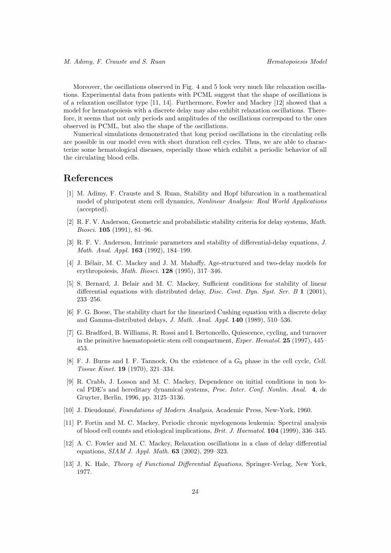
From Lemma 2.1, we conclude that E∗ is locally asymptotically stable when (34) holds.

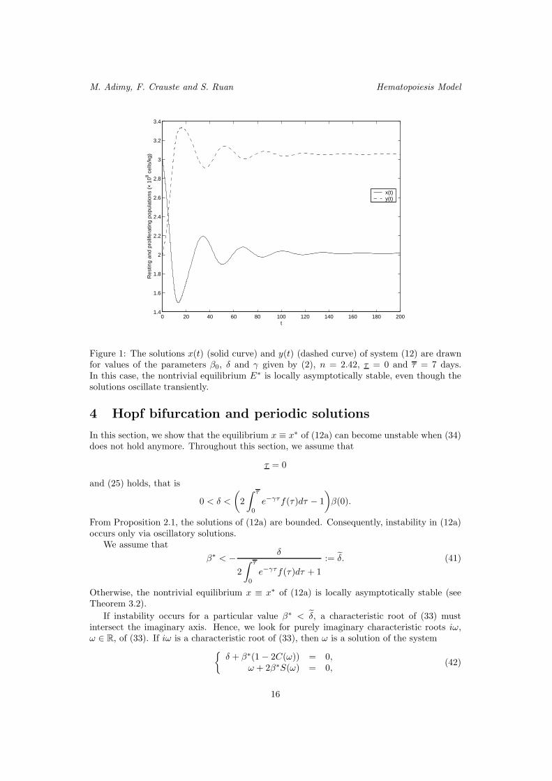
The asymptotic stability of E∗ is shown in Fig. 1. Values of the parameters are given by(2), except n = 2.42, τ = 0 and τ = 7 days. The function f is defined by

f(τ) =

1

τ − τ, if τ ∈ [τ, τ ],

0, otherwise.(40)

The Matlab solver for delay differential equations, dde23 [32], is used to obtain Fig. 1,as well as illustrations in Section 4 and Section 5.

When (34) does not hold, we have necessarily β∗ < 0. In this case, we cannot obtain thestability of E∗ for all values of β∗. In fact, in the next section we are going to show that theequilibrium E∗ can be destabilized, in this case, via a Hopf bifurcation.

15


0 20 40 60 80 100 120 140 160 180 2001.4

1.6

1.8

2

2.2

2.4

2.6

2.8

3

3.2

3.4

t

Res

ting

and

prol

ifera

ting

popu

latio

ns (

× 10

8 cel

ls/k

g)

x(t)y(t)

Figure 1: The solutions x(t) (solid curve) and y(t) (dashed curve) of system (12) are drawnfor values of the parameters β0, δ and γ given by (2), n = 2.42, τ = 0 and τ = 7 days.In this case, the nontrivial equilibrium E∗ is locally asymptotically stable, even though thesolutions oscillate transiently.

4 Hopf bifurcation and periodic solutions

In this section, we show that the equilibrium x ≡ x∗ of (12a) can become unstable when (34)does not hold anymore. Throughout this section, we assume that

τ = 0

and (25) holds, that is

0 < δ <

(2

∫ τ

0


)β(0).

From Proposition 2.1, the solutions of (12a) are bounded. Consequently, instability in (12a)occurs only via oscillatory solutions.

We assume that

β∗ < −δ

2

∫ τ

0


:= δ. (41)

Otherwise, the nontrivial equilibrium x ≡ x∗ of (12a) is locally asymptotically stable (seeTheorem 3.2).

If instability occurs for a particular value β∗ < δ, a characteristic root of (33) mustintersect the imaginary axis. Hence, we look for purely imaginary characteristic roots iω,ω ∈ R, of (33). If iω is a characteristic root of (33), then ω is a solution of the system

δ + β∗(1 − 2C(ω)) = 0,

ω + 2β∗S(ω) = 0,(42)

16


where

C(ω) :=

∫ τ

0

e−γτf(τ) cos(ωτ)dτ and S(ω) :=

∫ τ

0

e−γτf(τ) sin(ωτ)dτ.

One can notice that ω = 0 is not a solution of (42). Otherwise,

δ =

(2

∫ τ

0


)β∗ < 0,

which gives a contradiction. Moreover, if ω is a solution of (42), then −iω is also a charac-teristic root. Thus, we only look for positive solutions ω.

Lemma 4.1. Assume that the function τ 7→ e−γτf(τ) is decreasing. Then, for each δ such

that (25) is satisfied, (42) has at least one solution (β∗c , ωc), with β∗

c < δ and ωc > 0. Itfollows that (33) has at least one pair of purely imaginary roots ±iωc for β

∗ = β∗c . Moreover,

±iωc are simple characteristic roots of (33). Consider the branch of characteristic rootsλ(−β∗), such that λ(−β∗

c ) = iωc. Then

dRe(λ)

d(−β∗)

∣∣∣∣β∗=β∗

c

> 0 if and only if − δ

(S(ωc)

ωc

)′

> C′(ωc). (43)

Proof. First, we show by induction that S(ω) > 0 for ω > 0. It is clear that S(ω) > 0 ifωτ ∈ (0, π]. Suppose that ωτ ∈ (π, 2π]. Then

S(ω) =1

ω

∫ ωτ

0

e−γ τ

ω f( τω

)sin(τ)dτ

=1

ω

∫ π

0

e−γ τ

ω f( τω

)sin(τ)dτ +

1

ω

∫ ωτ

π

e−γ τ

ω f( τω

)sin(τ)dτ.

Since f is supported on the interval [0, τ ], it follows that

∫ 2π

ωτ

e−γ τ

ω f( τω

)sin(τ)dτ = 0.

So, we obtain

S(ω) =1

ω

∫ π

0

e−γ τ

ω f( τω

)sin(τ)dτ +

1

ω

∫ 2π

π

e−γ τ

ω f( τω

)sin(τ)dτ

=1

ω

∫ π

0

(e−γ τ

ω f( τω

)− e−γ τ+π

ω f(τ + π

ω

))sin(τ)dτ.

Since the function τ 7→ e−γτf(τ) is decreasing, we finally get S(ω) > 0. Using a similarargument for ωτ ∈ (kπ, (k + 1)π], with k ∈ N, k ≥ 2, we deduce that S(ω) > 0 for all ω > 0.

Consider the equation

g(ω) :=ω(1− 2C(ω)

)

2S(ω)= δ, ω > 0. (44)

The function g is continuous with

limω→0

g(ω) =1− 2C(0)

2

∫ τ

0

τe−γτf(τ)dτ

< 0 (45)

17


because (25) leads to 1− 2C(0) < 0. Moreover, the Riemann–Lebesgue’s lemma implies that

limω→+∞

C(ω) = limω→+∞

S(ω) = 0.

This yieldslim

ω→+∞g(ω) = +∞.

We conclude that there exists a solution ωc > 0 of (44). Since S(ωc) > 0 and g(ωc) = δ > 0,we obtain 1− 2C(ωc) > 0. Set

β∗c = −

δ

1− 2C(ωc)< 0. (46)

Since |C(ωc)| < C(0), it follows that

β∗c < −

δ

2C(0) + 1= δ.

One can check that (β∗c , ωc) is a solution of (42). It follows that ±iωc are characteristic roots

of (33) for β∗ = β∗c .

Define a branch of characteristic roots λ(−β∗) of (33) such that λ(−β∗c ) = iωc. We use

the parameter −β∗ because β∗ < δ < 0.Using (33), we obtain

[1 + 2β∗

∫ τ

0

τe−(λ+γ)τf(τ)dτ

]dλ

d(−β∗)= 1− 2

∫ τ

0

e−(λ+γ)τf(τ)dτ. (47)

If we assume, by contradiction, that iωc is not a simple root of (33), then (47) leads to

C(ωc) =1

2and S(ωc) = 0.

Since S(ωc) > 0, we obtain a contradiction. Thus, iωc is a simple root of (33).Moreover, using (47), we have

(dλ

d(−β∗)

)−1

=

1 + 2β∗

∫ τ

0


1− 2

∫ τ

0

e−(λ+γ)τf(τ)dτ

.

Since λ is a characteristic root of (33), we also have

1− 2

∫ τ

0

e−(λ+γ)τf(τ)dτ = −λ+ δ

β∗.

So, we deduce

(dλ

d(−β∗)

)−1

= −β∗

1 + 2β∗

∫ τ

0


λ+ δ.

18


Then,

sign

dRe(λ)

d(−β∗)

∣∣∣∣β∗=β∗

c

= sign

Re

(dλ

d(−β∗)

)−1∣∣∣∣β∗=β∗

c

= sign

Re

(− β∗

1 + 2β∗

∫ τ

0


λ+ δ

)∣∣∣∣β∗=β∗

c

= sign

− β∗

c

δ(1 + 2β∗cS

′(ωc)) + 2β∗cωcC

′(ωc)

δ2 + ω2c

= sign

δ(1 + 2β∗

cS′(ωc)) + 2β∗

cωcC′(ωc)

.

From (46) and the fact that 1− 2C(ωc) > 0, this leads to

sign

dRe(λ)

d(−β∗)

∣∣∣∣β∗=β∗

c

= sign

1− 2C(ωc)− 2δS′(ωc)− 2ωcC

′(ωc)

= sign

2ωc

(− C′(ωc)− δ

(S(ωc)

ωc

)′)

= sign

− C′(ωc)− δ

(S(ωc)

ωc

)′.

This concludes the proof.

Remark 2. Consider the function g defined by (44) and denote by α the quantity

α :=

(2

∫ τ

0


)β(0).

Define the sets

Ω := ω > 0; 0 < g(ω) < α and g′(ω) = 0 and Λ := g(Ω).

One can notice that Λ is finite (or empty). If δ ∈ (0, α) \ Λ, then

dRe(λ)

d(−β∗)

∣∣∣∣β∗=β∗

c

6= 0.

Indeed, we have

g′(ω) = −ω

S(ω)

(g(ω)

(S(ω)

ω

)′

+ C′(ω)

), ω > 0.

Since δ /∈ Λ, we have g′(ωc) 6= 0. Moreover, g(ωc) = δ. Thus

C′(ωc) 6= −δ

(S(ωc)

ωc

)′

.

We conclude by using (43).Lemma 4.1, together with Remark 2, allows us to state and prove the following theorem.

19


Theorem 4.1. Assume that the function τ 7→ e−γτf(τ) is decreasing. Then, for each δ /∈ Λ

satisfying (25), there exists β∗c < δ such that the equilibrium x ≡ x∗ is locally asymptotically

stable when β∗c < β∗ ≤ δ and a Hopf bifurcation occurs at x ≡ x∗ when β∗ = β∗

c .

Proof. First, recall that x ≡ x∗ is locally asymptotically stable when β∗ = δ (see Theorem3.2). We recall that, from the properties of the function g, equation (44) has a finite numberof solutions (see Lemma 4.1). We set

β∗c = −

δ

1− 2C(ω∗c ),

where ω∗c is the smaller positive real such that

C(ω∗c ) = minC(ω); ω is a solution of (44).

Then, β∗c is the maximum value of β∗ (as defined in Lemma 4.1) which gives a solution of

(42). From Lemma 4.1, (33) has no purely imaginary roots while β∗c < β∗ ≤ δ. Consequently,

Rouche’s Theorem [10, p.248] leads to the local asymptotic stability of x ≡ x∗.When β∗ = β∗

c , (33) has a pair of purely imaginary roots ±iωc, ωc > 0 (see Lemma 4.1).Moreover, since δ /∈ Λ, Remark 2 implies that

dRe(λ)

d(−β∗)

∣∣∣∣β∗=β∗

c

6= 0.

Assume, by contradiction, thatdRe(λ)

d(−β∗)< 0

for β∗ > β∗c , β

∗ close to β∗c . Then there exists a characteristic root λ(−β∗) such that

Reλ(−β∗) > 0. This contradicts the fact that x ≡ x∗ is locally asymptotically stable whenβ∗ > β∗

c . Thus, we obtaindRe(λ)

d(−β∗)

∣∣∣∣β∗=β∗

c

> 0.

This implies the existence of a Hopf bifurcation at x ≡ x∗ for β∗ = β∗c .

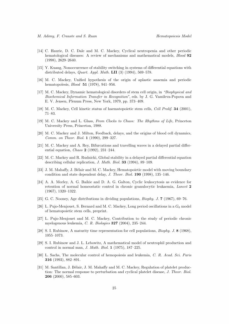
With the values of δ, γ and β0 given by (2), and τ = 7 days, (12) has periodic solutionsfor β∗

c = −0.3881 with a period about 33 days. This value of β∗c corresponds to n = 2.53 (see

Fig. 2 and 3). The function f is given by (40).The bifurcation parameter was chosen to be β∗ in this study, and the values of β∗ depend

strongly on the sensitivity n of the function β(x), since all other parameters are fixed by (25).In this model, the sensitivity n plays a crucial role in the appearance of periodic solutions.Pujo-Menjouet and Mackey [27] already noticed the influence of this parameter on system(12) when the delay is constant (or equivalently, when f is a Dirac measure). The sensitivityn describes the way the rate of introduction in the proliferating phase reacts to changes inthe resting phase population produced by external stimuli: a release of erythropoietin, forexample, or the action of some growth factors.

Of course, the influence of other parameters (like mortality rates δ and γ, or the minimumand maximum delays τ and τ ) on the appearance of periodic solutions could be studied.However, since periodic hematological diseases — defined and described in Section 5 —are supposed to be due to hormonal control destabilization (see [11]), then the parametern, among other parameters, seems to be appropriate to identify causes leading to periodicsolutions in (12).

20


0 20 40 60 80 100 120 140 160 180 2001

1.5

2

2.5

3

3.5

t

Res

ting

and

prol

ifera

ting

popu

latio

ns (

× 10

8 cel

ls/k

g)

x(t)y(t)

Figure 2: The solutions of system (12), x(t) (solid curve) and y(t) (dashed curve), are drawnwhen the Hopf bifurcation occurs. This corresponds to n = 2.53 with the other parametersgiven by (2) and τ = 7 days. Periodic solutions appear with period of the oscillations about33 days.

1.2 1.4 1.6 1.8 2 2.2 2.4 2.6 2.8 32

2.5

3

3.5

x(t)

y(t)

Figure 3: For the values used in Fig.2, the solutions are shown in the (x, y)-plane: thetrajectories reach a limit cycle, surrounding the equilibrium.

21


5 Discussion

Among the wide range of diseases affecting blood cells, periodic hematological diseases (Hau-rie et al. [14]) are of main importance because of their intrinsic nature. These diseases arecharacterized by significant oscillations in the number of circulating cells, with periods rang-ing from weeks (19–21 days for cyclical neutropenia [14]) to months (30 to 100 days for chronicmyelogenous leukemia [14]) and amplitudes varying from normal to low levels or normal tohigh levels, depending on the cells types [14]. Because of their dynamic character, periodichematological diseases offer an opportunity to understand some of the regulating processesinvolved in the production of hematopoietic cells, which are still not well-understood.

Some periodic hematological diseases involve only one type of blood cells, for example,red blood cells in periodic auto-immune hemolytic anemia (Belair et al. [4]) or platelets incyclical thrombocytopenia (Santillan et al. [31]). In these cases, periods of the oscillationsare usually between two and four times the bone marrow production delay. However, otherperiodic hematological diseases, such as cyclical neutropenia (Haurie et al. [14]) or chronicmyelogenous leukemia (Fortin and Mackey [11]), show oscillations in all of the circulatingblood cells, i.e., white cells, red blood cells and platelets. These diseases involve oscillationswith quite long periods (on the order of weeks to months). A destabilization of the pluripo-tential stem cell population (from which all of the mature blood cells types are derived) seemsto be at the origin of these diseases.

We focus, in particularly, on chronic myelogenous leukemia (CML), a cancer of the whitecells, resulting from the malignant transformation of a single pluripotential stem cell in thebone marrow (Pujo-Menjouet et al. [26]). As described in Morley et al. [24], oscillations canbe observed in patients with CML, with the same period for white cells, red blood cells andplatelets. This is called periodic chronic myelogenous leukemia (PCML). The period of theoscillations in PCML ranges from 30 to 100 days (Haurie et al. [14], Fortin and Mackey [11]),depending on patients. The difference between these periods and the average pluripotentialcell cycle duration (between 1 to 4 days, as observed in mouses, see Mackey [18]) is still notwell-understood.

Recently, to understand the dynamics of periodic chronic myelogenous leukemia, Pujo-Menjouet et al. [26] considered a model for the regulation of stem cell dynamics and investi-gated the influence of parameters in this stem cell model on the oscillations period when themodel becomes unstable and starts to oscillate. In this paper, taking into account the factthat a cell cycle has two phases, that is, stem cells in process are either in a resting phase oractively proliferating, and assuming that cells divide at different ages, we proposed a systemof differential equations with distributed delay to model the dynamics of hematopoietic stemcells. By constructing a Lyapunov functional, we gave conditions for the trivial equilibriumto be globally asymptotically stable. Local stability and Hopf bifurcation of the nontrivialequilibrium were studied, the existence of a Hopf bifurcation leading to the appearance ofperiodic solutions in this model, with a period around 30 days at the bifurcation.

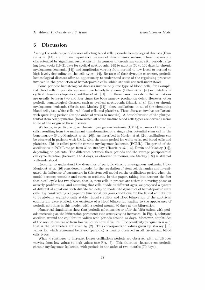
Numerical simulations show that periodic solutions occur after the bifurcation, with peri-ods increasing as the bifurcation parameter (the sensitivity n) increases. In Fig. 4, solutionsoscillate around the equilibrium values with periods around 45 days. Moreover, amplitudesof the oscillations range from low values to normal values. The sensitivity is equal to n = 3,that is the parameters are given by (2). This corresponds to values given by Mackey [16],values for which abnormal behavior (periodic) is usually observed in all circulating bloodcells types.

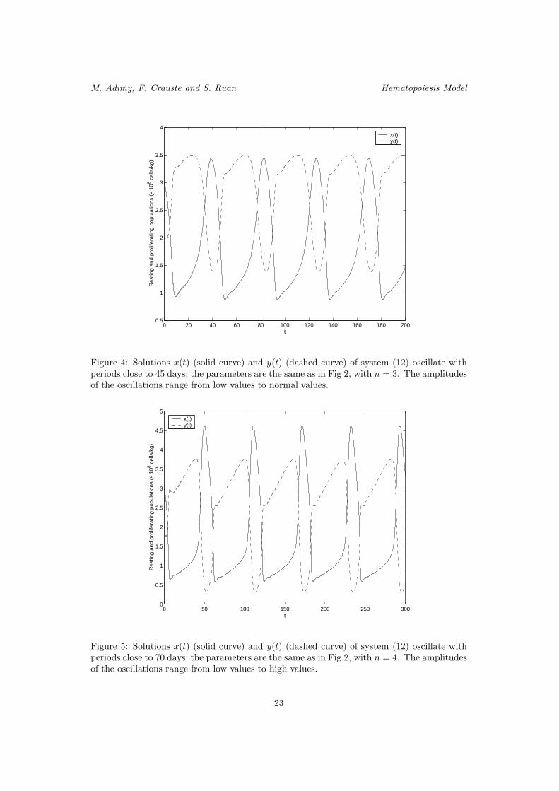
When n continues to increase, longer oscillations periods are observed with amplitudesvarying from low values to high values (see Fig. 5). This situation characterizes periodicchronic myelogenous leukemia, with periods in the order of two months (70 days).

22


0 20 40 60 80 100 120 140 160 180 2000.5

1

1.5

2

2.5

3

3.5

4

t

Res

ting

and

prol

ifera

ting

popu

latio

ns (

× 10

8 cel

ls/k

g)

x(t)y(t)

Figure 4: Solutions x(t) (solid curve) and y(t) (dashed curve) of system (12) oscillate withperiods close to 45 days; the parameters are the same as in Fig 2, with n = 3. The amplitudesof the oscillations range from low values to normal values.

0 50 100 150 200 250 3000

0.5

1

1.5

2

2.5

3

3.5

4

4.5

5

t

Res

ting

and

prol

ifera

ting

popu

latio

ns (

× 10

8 cel

ls/k

g)

x(t)y(t)

Figure 5: Solutions x(t) (solid curve) and y(t) (dashed curve) of system (12) oscillate withperiods close to 70 days; the parameters are the same as in Fig 2, with n = 4. The amplitudesof the oscillations range from low values to high values.

23


Moreover, the oscillations observed in Fig. 4 and 5 look very much like relaxation oscilla-tions. Experimental data from patients with PCML suggest that the shape of oscillations isof a relaxation oscillator type [11, 14]. Furthermore, Fowler and Mackey [12] showed that amodel for hematopoiesis with a discrete delay may also exhibit relaxation oscillations. There-fore, it seems that not only periods and amplitudes of the oscillations correspond to the onesobserved in PCML, but also the shape of the oscillations.

Numerical simulations demonstrated that long period oscillations in the circulating cellsare possible in our model even with short duration cell cycles. Thus, we are able to charac-terize some hematological diseases, especially those which exhibit a periodic behavior of allthe circulating blood cells.

References

[1] M. Adimy, F. Crauste and S. Ruan, Stability and Hopf bifurcation in a mathematicalmodel of pluripotent stem cell dynamics, Nonlinear Analysis: Real World Applications(accepted).

[2] R. F. V. Anderson, Geometric and probabilistic stability criteria for delay systems,Math.Biosci. 105 (1991), 81–96.

[3] R. F. V. Anderson, Intrinsic parameters and stability of differential-delay equations, J.Math. Anal. Appl. 163 (1992), 184–199.

[4] J. Belair, M. C. Mackey and J. M. Mahaffy, Age-structured and two-delay models forerythropoiesis, Math. Biosci. 128 (1995), 317–346.

[5] S. Bernard, J. Belair and M. C. Mackey, Sufficient conditions for stability of lineardifferential equations with distributed delay, Disc. Cont. Dyn. Syst. Ser. B 1 (2001),233–256.

[6] F. G. Boese, The stability chart for the linearized Cushing equation with a discrete delayand Gamma-distributed delays, J. Math. Anal. Appl. 140 (1989), 510–536.

[7] G. Bradford, B. Williams, R. Rossi and I. Bertoncello, Quiescence, cycling, and turnoverin the primitive haematopoietic stem cell compartment, Exper. Hematol. 25 (1997), 445–453.

[8] F. J. Burns and I. F. Tannock, On the existence of a G0 phase in the cell cycle, Cell.Tissue Kinet. 19 (1970), 321–334.

[9] R. Crabb, J. Losson and M. C. Mackey, Dependence on initial conditions in non lo-cal PDE’s and hereditary dynamical systems, Proc. Inter. Conf. Nonlin. Anal. 4, deGruyter, Berlin, 1996, pp. 3125–3136.

[10] J. Dieudonne, Foundations of Modern Analysis, Academic Press, New-York, 1960.

[11] P. Fortin and M. C. Mackey, Periodic chronic myelogenous leukemia: Spectral analysisof blood cell counts and etiological implications, Brit. J. Haematol. 104 (1999), 336–345.

[12] A. C. Fowler and M. C. Mackey, Relaxation oscillations in a class of delay differentialequations, SIAM J. Appl. Math. 63 (2002), 299–323.

[13] J. K. Hale, Theory of Functional Differential Equations, Springer-Verlag, New York,1977.

24


[14] C. Haurie, D. C. Dale and M. C. Mackey, Cyclical neutropenia and other periodichematological diseases: A review of mechanisms and mathematical models, Blood 92

(1998), 2629–2640.

[15] Y. Kuang, Nonoccurrence of stability switching in systems of differential equations withdistributed delays, Quart. Appl. Math. LII (3) (1994), 569–578.

[16] M. C. Mackey, Unified hypothesis of the origin of aplastic anaemia and periodichematopoıesis, Blood 51 (1978), 941–956.

[17] M. C. Mackey, Dynamic hematological disorders of stem cell origin, in “Biophysical andBiochemical Information Transfer in Recognition”, eds. by J. G. Vassileva-Popova andE. V. Jensen, Plenum Press, New York, 1979, pp. 373–409.

[18] M. C. Mackey, Cell kinetic status of haematopoietic stem cells, Cell Prolif. 34 (2001),71–83.

[19] M. C. Mackey and L. Glass, From Clocks to Chaos: The Rhythms of Life, PrincetonUniversity Press, Princeton, 1988.

[20] M. C. Mackey and J. Milton, Feedback, delays, and the origins of blood cell dynamics,Comm. on Theor. Biol. 1 (1990), 299–327.

[21] M. C. Mackey and A. Rey, Bifurcations and travelling waves in a delayed partial differ-ential equation, Chaos 2 (1992), 231–244.

[22] M. C. Mackey and R. Rudnicki, Global stability in a delayed partial differential equationdescribing cellular replication, J. Math. Biol. 33 (1994), 89–109.

[23] J. M. Mahaffy, J. Belair and M. C. Mackey, Hematopoietic model with moving boundarycondition and state dependent delay, J. Theor. Biol. 190 (1998), 135–146.

[24] A. A. Morley, A. G. Baikie and D. A. G. Galton, Cyclic leukocytosis as evidence forretention of normal homeostatic control in chronic granulocytic leukaemia, Lancet 2

(1967), 1320–1322.

[25] G. C. Nooney, Age distributions in dividing populations, Biophy. J. 7 (1967), 69–76.

[26] L. Pujo-Menjouet, S. Bernard and M. C. Mackey, Long period oscillations in a G0 modelof hematopoietic stem cells, preprint.

[27] L. Pujo-Menjouet and M. C. Mackey, Contribution to the study of periodic chronicmyelogenous leukemia, C. R. Biologies 327 (2004), 235–244.

[28] S. I. Rubinow, A maturity time representation for cell populations, Biophy. J. 8 (1968),1055–1073.

[29] S. I. Rubinow and J. L. Lebowitz, A mathematical model of neutrophil production andcontrol in normal man, J. Math. Biol. 1 (1975), 187–225.

[30] L. Sachs, The molecular control of hemopoiesis and leukemia, C. R. Acad. Sci. Paris316 (1993), 882–891.

[31] M. Santillan, J. Belair, J. M. Mahaffy and M. C. Mackey, Regulation of platelet produc-tion: The normal response to perturbation and cyclical platelet disease, J. Theor. Biol.206 (2000), 585–603.

25


[32] L. F. Shampine and S. Thompson, Solving DDEs in Matlab, Appl. Numer. Math. 37(2001), 441–458. http://www.radford.edu/∼thompson/webddes/.

[33] E. Trucco, Mathematical models for cellular systems: The Von Foerster equation, PartsI and II, Bull. Math. Biophys. 27 (1965), 285–304; 449–470.

[34] E. Trucco, Some remarks on changing populations, J. Ferm. Technol. 44 (1966), 218–226.

[35] G. F. Webb, Theory of nonlinear age-dependent population dynamics, Monographs andTextbooks in Pure and Applied Mathematics 89, Marcel Dekker Inc., New York, 1985.

26

http://www.radford.edu/~thompson/webddes/

Documents

AMathematical StudyoftheHematopoiesis ... · of hematopoiesis. We take into account the fact that a cell cycle has two phases, that We take into account the fact that a cell cycle