American Community Survey Design and Methodology (January

American Community Survey

Design and Methodology

(January 2014)

Chapter 10:

Data Preparation and

Processing for Housing Units

and Group Quarters

Version 2.0

January 30,

2014

ACS Design and Methodology (January 2014) – Chapter 10: Data Preparation and Processing Page ii

Version 2.0 January 30, 2014

[This page intentionally left blank]

ACS Design and Methodology (January 2014) – Chapter 10: Data Preparation and Processing Page iii


Table of Contents

Chapter 10: Data Preparation and Processing for Housing Units and Group Quarters ....... 1

10.1 Overview .......................................................................................................................... 1

10.2 Data Preparation ............................................................................................................... 2

10.3 Preparation for Creating Select Files and Edit Input Files ............................................. 19

10.4 Creating the Select Files and Edit Input Files. ............................................................... 21

10.5 Data Processing .............................................................................................................. 22

10.6 Editing and Imputation ................................................................................................... 22

10.7 Multiyear Data Processing ............................................................................................. 27

10.8 References ...................................................................................................................... 29

Figures

Figure 10-1: American Community Survey (ACS) Data Preparation and Processing ................... 2

Figure 10-2: Daily Processing of Housing Unit Data ..................................................................... 3

Figure 10-3: Monthly Data Capture File Creation .......................................................................... 5

Figure 10-4: American Community Survey (ACS) Coding ........................................................... 5

Figure 10-5: Backcoding................................................................................................................. 8

Figure 10-6: ACS Industry Questions............................................................................................. 9

Figure 10-7: ACS Industry Type Question ..................................................................................... 9

Figure 10-8: ACS Occupation Questions ..................................................................................... 10

Figure 10-9: Industry and Occupation (I/O) Coding .................................................................... 11

Figure 10-10: ACS Migration Questions ...................................................................................... 14

Figure 10-11: ACS Place-of-Work Questions .............................................................................. 15

Figure 10-12: Geocoding .............................................................................................................. 18

Figure 10-13: Acceptability Index ................................................................................................ 20

Figure 10-14: Multiyear Edited Data Process ............................................................................... 28

ACS Design and Methodology (January 2014) – Chapter 10: Data Preparation and Processing Page iv


Tables

Table 10-1: Type and Method of Coding ....................................................................................... 6

Table 10-2: Geographic Level of Specificity for Geocoding ....................................................... 16

Table 10-3: Percentage of Geocoding Cases With Automated Matched Coding ......................... 17

ACS Design and Methodology (January 2014) – Chapter 10: Data Preparation and Processing Page 1


Chapter 10: Data Preparation and Processing for Housing Units and

Group Quarters

10.1 Overview

Data preparation and processing are critical steps in the survey process, particularly in terms of

improving data quality. It is typical for developers of a large ongoing survey, such as the

American Community Survey (ACS) to develop stringent procedures and rules to guide these

processes and ensure that they are done in a consistent and accurate manner. This chapter

discusses the actions taken during ACS data preparation and processing, provides the reader with

an understanding of the various stages involved in readying the data for dissemination, and

describes the steps taken to produce high-quality data.

The main purpose of data preparation and processing is to take the response data gathered from

each survey collection mode to the point where they can be used to produce survey estimates.

Data returning from the field typically arrive in various stages of completion, from a completed

interview with no problems to one with most or all of the data items left blank. There can be

inconsistencies within the interviews, such that one response contradicts another, or duplicate

interviews may be returned from the same household but contain different answers to the same

question.

Upon arrival at the U.S. Census Bureau, all data undergo data preparation, where responses

from different modes are captured in electronic form creating Data Capture Files. The write-in

entries from the Data Capture Files are then subject to monthly coding operations. When the

monthly Data Capture Files are accumulated at year-end, a series of steps are taken to produce

Edit Input Files. These are created by merging operational status information (such as whether

the unit is vacant, occupied, or nonexistent) for each housing unit (HU) and group quarters

(GQ) facility with the files that include the response data. These combined data then undergo a

number of processing steps before they are ready to be tabulated for use in data products.

Figure 10-1 depicts the overall flow of data as they pass from data collection operations through

data preparation and processing and into data products development. While there are no set

definitions of data preparation versus data processing, all activities leading to the creation of the

Edit Input Files are considered data preparation activities, while those that follow are

considered data processing activities.



Figure 10-1: American Community Survey (ACS) Data Preparation and Processing

10.2 Data Preparation

The ACS control file is integral to data preparation and processing because it provides a single

database for all units in the sample. The control file includes detailed information documenting

operational outcomes for every ACS sample case. For the mail/internet operations, it documents

the receipt and check-in date of questionnaires returned by mail or the date completed on the

internet. The status of data capture for questionnaires and the results of the Failed-Edit Follow-

up (FEFU) operation also are recorded in this file. Chapter 7 provides a detailed discussion of

mail data collection, as well as computer-assisted telephone interview (CATI) and computer-

assisted personal interview (CAPI) operations.

For CAPI operations, the ACS control file stores information on whether or not a unit was

determined to be occupied or vacant. Data preparation, which joins together each case’s

control file information with the raw, unedited response data, involves three operations:

creation and processing of data capture files, coding, and creation of edit input files.

Creation and Preparation of Data Capture Files

Many processing procedures are necessary to prepare the ACS data for tabulation. In this section,

we examine each data preparation procedure separately. These procedures occur daily or

monthly, depending on the file type (control or data capture) and the data collection mode

(mail/internet, CATI, or CAPI). The processing that produces the final input files for data

products is conducted on a yearly basis.

Daily Data Processing

The HU data are collected on a continual basis throughout the year by mail/internet, CATI, and

CAPI. Sampled households first are mailed a request to complete their form on the internet and

then are subsequently mailed the ACS questionnaire. Households that do not complete their

form by mail/internet self-response and for which a phone number is available receive

telephone follow-up. As discussed in Chapter 7, a sample of the non-completed CATI cases is

sent to the field for in-person CAPI interviews, together with a sample of cases that could not



be mailed. Each day, the status of each sample case is updated in the ACS control file based on

data from data collection and capture operations. While the control file does not record

response data, it does indicate when cases are completed so as to avoid additional attempts

being made for completion in another mode.

The creation and processing of the data depends on the mode of data collection. Figure 10-2

shows the monthly processing of HU response data. Data from questionnaires received by

mail/internet are processed daily and are added to a Data Capture File (DCF) on a monthly basis.

Data received by mail/internet are run through a computerized process that checks for sufficient

responses and for large households that require follow-up. Cases failing the process are sent to

the FEFU operation. As discussed in more detail in Chapter 7, the mail version of the ACS asks

for detailed information on up to five household members. If there are more than five members

in the household, the FEFU process also will ask questions about those additional household

members. Telephone interviewers call the cases with missing or inconsistent data for corrections

or additional information. The FEFU data are also included in the data capture file as

mail/internet responses. The Telephone Questionnaire Assistance (TQA) operation uses the

CATI instrument to collect data. These data are also treated as mail responses as shown in Figure

10-2.

Mail

responses

CATI CAPI

ACS control file

Automated

clerical edit

Pass edit?

No

Failed edit

follow-up (FEFU)

Telephone

Questionnaire

Assistance

(TQA)

Yes

FEFU

responses

for data

capture file

TQA

responses

for data

capture file

CATI

responses

for data

capture file

CAPI

responses

for data

capture file

Figure 10-2: Daily Processing of Housing Unit Data



CATI follow-up is conducted at three telephone call centers. Data collected through telephone

interviews are entered into a BLAISE instrument. Operational data are transmitted to the Census

Bureau headquarters daily to update the control file with the current status of each case. For data

collected via the CAPI mode, Census Bureau field representatives (FRs) enter the ACS data

directly into a laptop during a personal visit to the sample address. The FR transmits completed

cases from the laptop to headquarters using an encrypted Internet connection. The control file

also is updated with the current status of the case. Each day, status information for GQs is

transmitted to headquarters for use in updating the control file. The GQ data are collected on

paper forms that are sent to the National Processing Center on a flow basis for data capture or

from a CAPI collection operation.

Monthly Data Processing

At the end of each month, a centralized DCF is augmented with the mail, CATI, and CAPI data

collected during the past month. These represent all data collected during the previous month,

regardless of the sample month for which the HU or GQ was chosen. Included in these files of

mail responses are FEFU files, both cases successfully completed and those for which the

required number of attempts have been made without successful resolution. As shown in Figure

10-3, monthly files from CATI and CAPI, along with the mail/internet self response, are used as

input files in doing the monthly data capture file processing.

At headquarters, the centralized DCF is used to store all ACS response data. During the creation

of the DCF, responses are reviewed and illegal values responses are identified. Responses of

‘‘Don’t Know’’ and ‘‘Refused’’ are identified as ‘‘D’’ and ‘‘R.’’ Illegal values are identified by

an ‘‘I,’’ and data capture rules cause some variables to be changed from illegal values to legal

values (Diskin, 2007c). An example of an illegal value would occur when a respondent leaves

the date of birth blank but gives ‘‘Age’’ as 125. This value is above the maximum allowable

value of 115. This variable would be recoded as age of 115 (Diskin, 2007a). Another example

would be putting a ‘‘19’’ in front of a four-digit year field where the respondent filled in only the

last two digits as ‘‘76’’ (Jiles, 2007). A variety of these data capture rules are applied as the data

are keyed in from mail questionnaires, and these same illegal values would be corrected by

telephone and field interviewers as they complete the interview. The same rules are applied to

internet responses through an automated set of business rules and are grouped in with the mail

data in the capture files. Once the data capture files have gone through this initial data cleaning,

the next step is processing the HU questions that require coding.



Figure 10-3: Monthly Data Capture File Creation

Coding

The ACS questionnaire includes a set of questions that offer the possibility of write-in responses,

each of which requires coding to make it machine-readable. Part of the preparation of newly

received data for entry into the DCF involves identifying these write-in responses and placing

them in a series of files that serve as input to the coding operations. The DCF monthly files

include HU and GQ data files, as well as a separate file for each write-in entry. The HU and GQ

write-ins are stored together. Figure 10-4 diagrams the general ACS coding process.

Figure 10-4: American Community Survey (ACS) Coding

FEFU

Responses

for Data

Capture File

Mail/Internet

Responses

for Data

Capture File

Monthly

Data

Capture

File

CATI

Responses

for Data

Capture File

TQA

Responses

for Data

Capture File

Coding

CAPI

Responses

for Data

Capture File

Monthly Data

Capture File

Backcoding

(automated then

clerical)

Geocoding

(automated then

clerical)

Coding

Database

Industry and

Occupation Coding

(automated then

clerical)



During the coding phase for write-in responses, fields with write-in values are translated into a

prescribed list of valid codes. The write-ins are organized into three types of coding: backcoding,

industry and occupation coding, and geocoding. All three types of ACS coding are automated

(i.e., use a series of computer programs to assign codes), clerically coded (coded by hand), or

some combination of the two. The items that are sent to coding along with the type and method

of coding, are illustrated below in Table 10-1.

Table 10-1: Type and Method of Coding

Item Type of Coding Method of Coding

Race ............................................... Backcoding Automated with clerical follow-up Hispanic Origin .............................. Backcoding Automated with clerical follow-up Ancestry ....................................... Backcoding Automated with clerical follow-up Language ....................................... Backcoding Automated with clerical follow-up Health Insurance ........................... Backcoding Automated with clerical follow-up Field of Degree .............................. Backcoding Automated with clerical follow-up Computer Types ............................ Backcoding Automated with clerical follow-up Internet Service ............................. Backcoding Automated with clerical follow-up Industry ......................................... Industry Automated with clerical follow-up Occupation .................................... Occupation Automated with clerical follow-up Place of Birth ................................. Geocoding Automated with clerical follow-up Migration ...................................... Geocoding Automated with clerical follow-up Place of Work ................................ Geocoding Automated with clerical follow-up

In 2013, the ACS added an internet option for response. The autocoding and clerk clerical coding

processes have remained the same as for all modes of response. However, the Census Bureau

anticipates the rules to change for converting internet response text to data files or for keying

mail response text to data files. Rule changes may affect the treatment of special characters (e.g.,

colons), resulting in a decrease in the match rate of incoming responses to the autocoder data

dictionaries, which are based on the current rules. If rule changes occur, then the autocoder may

add a process to adjust the incoming text data to match the data dictionaries. For example, the

process could remove special characters allowed under the new rules. For records that still

require clerk coding after autocoding, the new special characters would be retained and provided

to the clerks. If changes occur that affect any part of the industry and occupation coding

processes, future editions of this report will discuss the processing adjustments in detail.

Backcoding

The first type of coding is the one involving the most items—backcoding. Backcoded items are

those that allow for respondents to write in some response other than the categories listed.

Although respondents are instructed to mark one or more of the 12 given race categories on the

ACS form, they also are given the option to check ‘‘Some Other Race,’’ and to provide write-in

responses. For example, respondents are instructed that if they answer ‘‘American Indian or



Alaska Native,’’ they should print the name of their enrolled or principal tribe; this allows for a

more specific race response. Figure 10-5 illustrates backcoding processes.

All backcoded items go through an automated process for the first pass of coding. The written-in

responses are keyed into digital data and then matched to a data dictionary. The data dictionary

contains a list of the most common responses, with a code attached to each. The coding program

attempts to match the keyed response to an entry in the dictionary to assign a code. For example,

the question of language spoken in the home is automatically coded to one of 380 language cat-

egories. These categories were developed from a master code list of 55,000 language names and

variations. If the respondent lists more than one non-English language, only the first language is

coded.

However, not all cases can be assigned a code using the automated coding program. Responses

with misspellings, alternate spellings, or entries that do not match the data dictionary must be

sent to clerical coding. Trained human coders will look at each case and assign a code.

One example of a combination of autocoding and follow-up clerical coding is the ancestry item.

The write-in string for ancestry is matched against a census file containing all of the responses

ever given that have been associated with codes. If there is no match, an item is coded

manually. The clerical coder looks at the partial code assigned by the automatic coding program

and attempts to assign a full code.

To ensure that coding is accurate, a percentage of the backcoded items are sent through the

quality assurance (QA) process. The algorithm is specified according to the number of returns in

a batch. Batches of 1,000 randomly selected cases are sent to two QA coders who independently

assign codes. If the codes they assign do not match one another, or the codes assigned by the

automated coding program or clerical coder do not match, the case is sent to adjudication.

Adjudicator coders are coding supervisors with additional training and resources. The

adjudicating coder decides the proper code, and the case is considered complete.



Figure 10-5: Backcoding



Industry and Occupation Coding

The second type of coding is industry and occupation coding, which is slightly different from

backcoding. The ACS collects information concerning many aspects of the respondents’ work,

including commute time and mode of transportation to work, salary, and type of organization

employing the household members. To give a clear picture of the kind of work in which the

resident population is engaged, the ACS also asks about industry and occupation. Industry

information relates to the person’s employing organization and the kind of business it conducts.

Occupation is the work the person does for that organization. To aid in coding the industry and

occupation write-in questions, two additional supporting questions are asked—one before the

industry question and one after the occupation question. The wording for the industry and

occupation questions are shown in Figures 10-6, 10-7, and 10-8.

Figure 10-6: ACS Industry Questions

Figure 10-7: ACS Industry Type Question



Figure 10-8: ACS Occupation Questions

From these questions, monthly processing converts industry and occupation write-in responses to

a code category. Prior to 2012, specialized industry and occupation coders assigned all codes.

Industry and occupation items did not go through an automated assignment process. Beginning

with the 2012 data collection, industry and occupation coding incorporated automated

assignment as a first step in coding. This industry and occupation autocoder is a set of logistic

regression models, data dictionaries, and consistency edits (“hardcodes”) developed from around

two million clerk-coded records, including group quarters and Spanish records (Thompson, et al.,

2012). The autocoder assigns an industry or occupation code if the quality score, based on

agreement with clerk-coded records, is sufficiently high. If one or both of industry or occupation

remain unassigned, these residual records are then assigned a code by specialized industry and

occupation clerical coders. When clerical coders are unable to assign a code, the case is sent to

an expert, or coding referralist, for a decision. Once these cases are assigned both an industry and

an occupation code, they are placed in the general pool of completed responses. Both the

autocoder and the clerical coding have independent quality check processes. Figure 10-9

illustrates the industry and occupation coding process beginning with 2012 data.



Figure 10-9: Industry and Occupation (I/O) Coding



Both the automated and clerical industry and occupation coding use the Census Classification

System to code responses. This system is based on the North American Industry Classification

System (NAICS) for industry and the Standard Occupational Classification (SOC) for

occupation. The Census Classification System’s 4-digit code categories can be bridged directly

to the NAICS and SOC for comparisons. However, the degree of correspondence between the

systems may vary, depending on the level of specificity of responses collected on the ACS. For

instance, some 4-digit Census industry codes correspond to a 2-digit NAICS industry sector,

while others correspond to a 6-digit NAICS U.S. industry. Similarly, some 4-digit Census

occupation codes correspond to a 3-digit SOC minor occupation group, while others correspond

to a 6-digit SOC detailed occupation.

Standardized procedures and additional resources are maintained to aid in the assigning of

industry and occupation codes. Both the autocoder and clerical coders are given access to

additional responses, such as education level, age, and geographic location. Clerks may also use

an alphabetical index of industries and occupations. If the name of the company or business for

which a person works is available, clerical coders can look up the name on a reference listing of

employers and their industries. The Census Bureau has used many versions of this reference list,

often referred to as the Employer Name List (ENL). Some ENLs have been developed from

public publications while others have used previously coded records. There are also dedicated

clerks who code group quarters records and Spanish records. Finally, the coding referralists have

access to even more resources, including access to state registries and use of the Internet for

finding more information about the response.

Both the autocoder and clerical coders are subjected to regular quality checks. The autocoder

quality control (QC) process begins with referralists coding a sample of autocoded records

without seeing the autocoder’s assigned code. The two codes are compared and when they

disagree, a third code is assigned by a different referralist who sees both the autocoder’s and

first referralist’s codes. This third code is then used in final comparisons as the “correct” code.

If the autocoder agrees with the third code, it is considered to be correct, otherwise, the

autocoder is considered to be in error. Analysts then review industry or occupation categories

with high error rates, looking for patterns in word combinations that yield incorrect autocodes.

These “wordbits” are then recoded by referralists, and analysts test these new codes in the data

dictionaries and autocoding computer programs, updating them if appropriate.

The clerk quality assurance (QA) process begins with a sample of each coder’s records being

independently assigned by a different clerk who does not see the assigned code. Prior to 2012,

this sample was a fixed percentage of each clerk’s coded cases. Since June 2012, the sampling

rate is dynamic, based on the number of records a clerk codes in a month. The sample must also

meet a minimum sample size. After the samples are re-coded, the codes then are reconciled to

determine which is correct. Coders are required to maintain a high monthly agreement rate and

a minimum production rate to remain qualified to code. A coding supervisor oversees the QA

process.



Geocoding

The third type of coding that ACS uses is geocoding. This is the process of assigning a

standardized code to geographic data. Place-of-birth, migration, and place-of-work responses

require coding of a geographic location. These variables can be as localized as a street address

or as general as a country of origin (Boertlein, 2007b).1

The first category is place-of-birth coding, a means of coding responses to a U.S. state, the

District of Columbia, Puerto Rico, a specific U.S. Island Area, or a foreign country where the

respondents were born (Boertlein, 2007b). These data are gathered through a two-part question

on the ACS asking where the person was born and in what state (if in the United States) or

country (if outside the United States).

The second category of geocoding, migration coding, again requires matching the write-in

responses of state, foreign country, county, city, inside/outside city limits, and ZIP code given by

the respondent to geocoding reference files and attaching geographic codes to those responses. A

series of three questions collects these data and are shown in Figure 10-10.

1 The following sections dealing with geocoding rely heavily on Boertlein (2007b).



Figure 10-10: ACS Migration Questions

First, respondents are asked if they lived at this address a year ago; if the respondent answers no,

there are several follow-up questions, such as the name of the city, country, state, and ZIP code

of the previous home.

The goal of migration coding is to code responses to a U.S. state, the District of Columbia,

Puerto Rico, U.S. Island Area or foreign country, a county (municipio in Puerto Rico), a Minor

Civil Division (MCD) in 12 states, and place (city, town, or post office). The inside/outside city

limits indicator and the ZIP code responses are used in the coding operations but are not a part of

the final outgoing geographic codes.

The final category of geocoding is place-of-work (POW) coding. The POW coding questions and

the question for employer’s name are shown Figure 10-11.



Figure 10-11: ACS Place-of-Work Questions

The ACS questionnaire first establishes whether the respondent worked in the previous week. If

this question is answered ‘‘Yes,’’ follow-up questions regarding the physical location of this

work are asked.



The POW coding requires matching the write-in responses of structure number and street name

address, place, inside/outside city limits, county, state/foreign country, and ZIP code to reference

files and attaching geographic codes to those responses. If the street address location information

provided by the respondent is inadequate for geocoding, the employer’s name often provides the

necessary additional information. Again, the inside/outside city limits indicator and ZIP code

responses are used in the coding operations but are not a part of the final outgoing geographic

codes.

Each of the three geocoding items is coded to different levels of geographic specificity. While

place-of-birth geocoding concentrates on larger geographic centers (i.e., states and countries), the

POW and migration geocoding tend to focus on more specific data. Table 10-2 is an outline of

the specificity of geocoding by type.

Table 10-2: Geographic Level of Specificity for Geocoding

Foreign countries States and Counties and

Desired precision— (including: provinces,

statistically statistically

Census

geocoded items continents, and equivalent equivalent ZIP designated Block

regions) entities entities codes places levels

Place of birth ........ X X

Migration ......... X X X X

Place of work ........ X X X X X X

The main reference file used for geocoding is the State and Foreign Country File (SFCF). The

SFCF contains two key pieces of information for geocoding. They are:

The names and abbreviations of each state, the District of Columbia, Puerto Rico, and the

U.S. Island Areas.

The official names, alternate names, and abbreviations of foreign countries and selected

foreign city, state, county, and regional names.

Other reference files (such as a military installation list and City Reference File) are available

and used in instances where ‘‘the respondent’s information is either inconsistent with the

instructions or is incomplete’’ (Boertlein, 2007b).

Responses do not have to match a reference file entry exactly to meet requirements for a correct

geocode. The coding algorithm for this automated geocoding allows for equivocations, such as

using Soundex values of letters (for example, m=n, f=ph) and reversing consecutive letter

combinations (ie=ei). Each equivocation is assigned a numeric value, or confidence level, with

exact matches receiving the best score or highest confidence (Boertlein, 2007b). A preference is

given for matches that are consistent with any check boxes marked and/or response boxes filled.

The responses have to match a reference file entry with a relatively high level of confidence for

the automated match to be accepted. Soundex values are used for most types of geocoding and



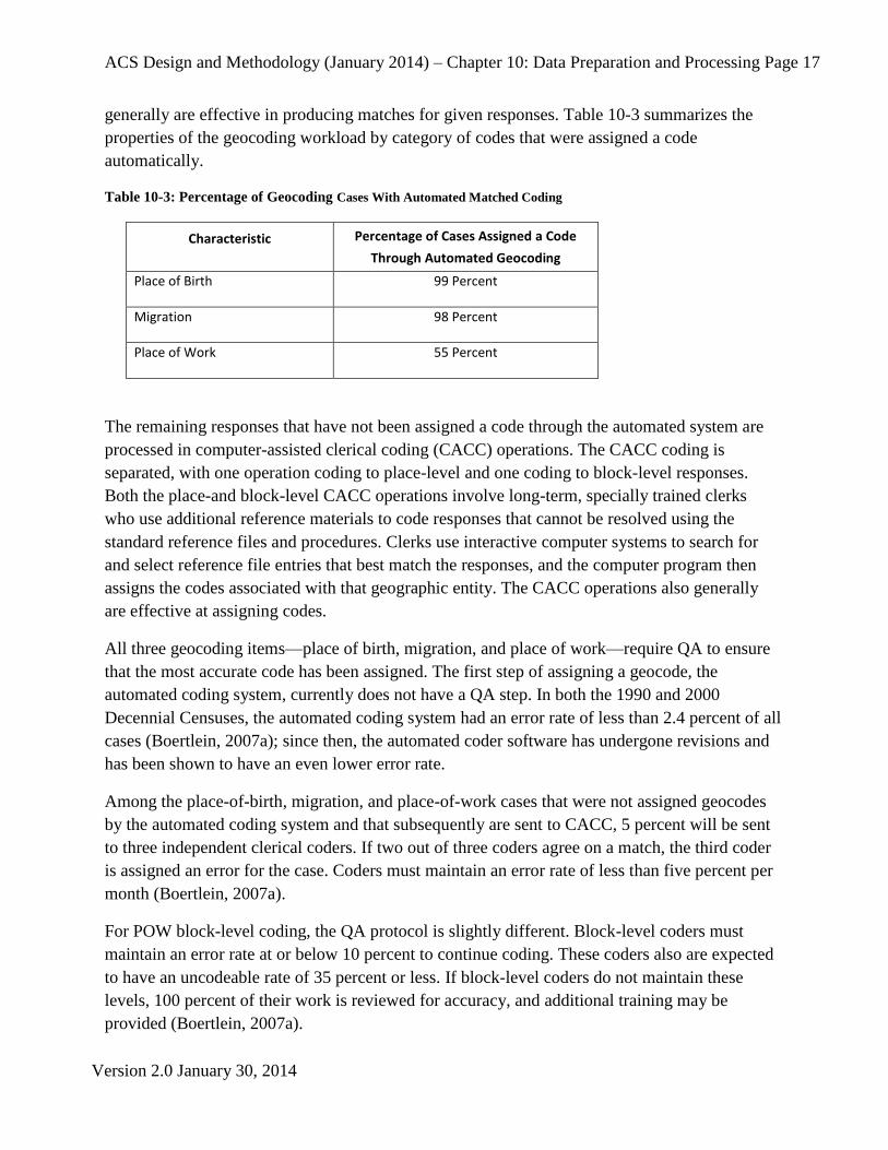
generally are effective in producing matches for given responses. Table 10-3 summarizes the

properties of the geocoding workload by category of codes that were assigned a code

automatically.

Table 10-3: Percentage of Geocoding Cases With Automated Matched Coding

Characteristic Percentage of Cases Assigned a Code

Through Automated Geocoding

Place of Birth 99 Percent

Migration 98 Percent

Place of Work 55 Percent

The remaining responses that have not been assigned a code through the automated system are

processed in computer-assisted clerical coding (CACC) operations. The CACC coding is

separated, with one operation coding to place-level and one coding to block-level responses.

Both the place-and block-level CACC operations involve long-term, specially trained clerks

who use additional reference materials to code responses that cannot be resolved using the

standard reference files and procedures. Clerks use interactive computer systems to search for

and select reference file entries that best match the responses, and the computer program then

assigns the codes associated with that geographic entity. The CACC operations also generally

are effective at assigning codes.

All three geocoding items—place of birth, migration, and place of work—require QA to ensure

that the most accurate code has been assigned. The first step of assigning a geocode, the

automated coding system, currently does not have a QA step. In both the 1990 and 2000

Decennial Censuses, the automated coding system had an error rate of less than 2.4 percent of all

cases (Boertlein, 2007a); since then, the automated coder software has undergone revisions and

has been shown to have an even lower error rate.

Among the place-of-birth, migration, and place-of-work cases that were not assigned geocodes

by the automated coding system and that subsequently are sent to CACC, 5 percent will be sent

to three independent clerical coders. If two out of three coders agree on a match, the third coder

is assigned an error for the case. Coders must maintain an error rate of less than five percent per

month (Boertlein, 2007a).

For POW block-level coding, the QA protocol is slightly different. Block-level coders must

maintain an error rate at or below 10 percent to continue coding. These coders also are expected

to have an uncodeable rate of 35 percent or less. If block-level coders do not maintain these

levels, 100 percent of their work is reviewed for accuracy, and additional training may be

provided (Boertlein, 2007a).



The QA system for ACS geocoding also includes feedback to the coders. Those with high error

rates or high uncodeable rates, as well as those who have low production rates or make consis-

tent errors, may be offered additional training or general feedback on how to improve.

Figure 10-12 illustrates automatic geocoding.

Figure 10-12: Geocoding



10.3 Preparation for Creating Select Files and Edit Input Files

The final data preparation operation involves creating Select Files and Edit Input Files for data

processing. To create these files, a number of preparatory steps must be followed. By the end of

the year, the response data stored in the DCF will have been updated 12 times and will become a

principal source for the edit-input process. Coding input files are created from the DCF files of

write-in entries. Edit Input Files combine data from the DCF files and the returned coding files,

and operational information for each case is merged with the ACS control file. The resulting file

includes housing and person data. Vacant units are included, as they may have some housing

data.

Creation of the Select and Edit Input Files involves carefully examining several components of

the data, each described in more detail below. First, the response type and number of people in

the household unit are assessed to determine inconsistencies. Second, the return is examined to

establish if there are enough data to count the return as complete, and third, any duplicate returns

undergo a process of selection to assess which return will be used.

Response Type and Number of People in the HU

Each HU is assigned a response type that describes its status as occupied, temporarily

occupied, vacant, a delete, or noninterview. Deleted HUs are units that are determined to be

nonexistent, demolished, or commercial units, i.e., out of scope for the ACS.

While this type of classification already exists in the DCF, it can be changed from ‘‘occupied’’

to ‘‘vacant’’ or even to ‘‘noninterview’’ under certain circumstances, depending on the final

number of persons in the HU, in combination with other variables. In general, if the return

indicates that the HU is not occupied and that there are no people listed with data, the record and

number of people (which equals 0) is left as is. If the HU is listed as occupied, but the number of

persons for whom data are reported is 0, it is considered vacant.

The data also are examined to determine the total number of people living in the HU, which is

not always a straightforward process. For example, on a mail return, the count of people on the

cover of the form sometimes may not match the number of people reported inside. Another

inconsistency would be when more than five members are listed for the HU, and the FEFU fails

to get information for any additional members beyond the fifth. In this case, there will be a

difference between the number of person records and the number of people listed in the HU. To

reconcile the numbers, several steps are taken, but in general, the largest number listed is used.

(For more details on the process, see Powers [2012].)

Determining if a Return Is Acceptable

The acceptability index is a data quality measure used to determine if the data collected from an

occupied HU or a GQ are complete enough to include a person record. Figure 10-13 illustrates

the acceptability index. Six basic demographic questions plus marital status are examined for



answers. One point is given for each question answered for a total of seven possible points that

could be assigned to each person in the household. A person with a response to either age or date

of birth scores two points because given one, the other can be derived or assigned. The total

number of points is then divided by the total number of household members. For the interview to

be accepted, there must be an average of 2.5 responses per person in the household. Household

records that do not meet this acceptability index are classified as noninterviews and will not be

included in further data processing. These cases will be accounted for in the weighting process,

as described in Chapter 11.

Figure 10-13: Acceptability Index

If the Acceptability Index is greater than 2.5, the person record is accepted as a complete return.

If the Acceptability Index is less than 2.5, the person record is not accepted as a complete return.

Unduplicating Multiple Returns

Once the universe of acceptable interviews is determined, the HU data are reviewed to

unduplicate multiple returns for a single HU. There are several reasons why more than one

response can exist for an HU. A household might return two mail/internet forms, one in response

to the request to complete by internet, and a second in response to the replacement mailing.

Depending on the timing, a household might return an internet response or mailed form, but also

be interviewed in CATI or CAPI before the internet or mail form is logged in as returned. If

more than one return exists for an HU, a quality index is used to select one as the final return.

This index is calculated as the percentage of items with responses out of the total number of

items that should have been completed. The index considers responses to both population and

housing items.

The mode of each return also is considered in the decision regarding which of two returns to

accept, with preference generally given to mail/internet returns. For the more complete set of

rules, see Powers (2012).

After the resolution of multiple returns, each sample case is assigned a value for three critical

variables—data collection mode, month of interview, and case status. The month in which data



were collected from each sample case is determined and then used to define the universe of cases

to be used in the production of survey estimates. For example, data collected in January 2013

were included in the 2012 ACS data products released in 2013 because the data collected were

associated with the 2012 ACS data collection. Similarly, data collected in December 2013 as part

of the 2014 ACS will be included with the 2014 ACS data products that are released in 2015

because the data collected are associated with the 2014 ACS data collection.

10.4 Creating the Select Files and Edit Input Files.

Select Files

Select Files are the series of files that pertain to those cases that will be included in the Edit Input

File. As noted above, these files include the case status, the interview month, and the data collec-

tion mode for all cases. The largest select file, also called the Omnibus Select File, contains

every available case from 14 months of sample—the current (selected) year and November and

December of the previous year. This file includes acceptable and unacceptable returns.

Unacceptable returns include initial sample cases that were subsampled out at the CAPI stage,2

returns that were too incomplete to meet the acceptability requirements. In addition, while the

‘‘current year’’ includes all cases sampled in that year, not all returns from the sampled year

were completed in that year. This file is then reduced to include only occupied housing units and

vacant units that are to be tabulated in the current year. That is, returns that were tabulated in the

prior year, or will be tabulated in the next year, are excluded. The final screening removes

returns from vacant boats because they are not included in the ACS estimation universe.

Edit Input Files

The next step is the creation of the Housing Edit Input File and the Person Edit Input File. The

Housing Edit Input file is created by first merging the DCF household data with the codes for

computer and internet access. This file is then merged with the Final Accepted Select File with

the DCF housing data. Date variables then are modified into the proper format. Next, variables

are given the prefix ‘‘U,’’ followed by the variable name to indicate they are unedited variables.

Finally, answers that are ‘‘Don’t Know’’ and ‘‘Refuse’’ are set as missing blank values for the

edit process.

The Person Edit Input File is created by first merging the DCF person data with the codes for

Hispanic origin, race, ancestry, language, field of degree, place of work, health insurance, and

current or most recent job activity. This file then is merged with the Final Accepted Select File to

create a file with all person information for all accepted HUs. As was done for the housing items,

2 See Chapter 7 for a full discussion of subsampling and the ACS



the person items are set with a ‘‘U’’ in front of the variable name to indicate that they are

unedited variables. Next, various name flags are set to identify people with Spanish surnames

and those with ‘‘non-name’’ first names, such as ‘‘female’’ or ‘‘boy.’’ When the adjudicated

number of people in an HU is greater than the number of person records, blank person records

are created for them. The data for these records will be filled in during the imputation process.

Finally, as with the housing variables, ‘‘Don’t Know’’ and ‘‘Refuse’’ answers are set as missing

blank values for the edit process. When complete, the Edit Input Files encompass the information

from the DCF housing and person files but only for the unduplicated response records with data

collected during the calendar year.

10.5 Data Processing

Once the Edit Input Files have been generated and verified, the edit and imputation

process begins. The main steps in this process are:

Editing and imputation

Generating recoded variables

Reviewing edit results

Creating input files for data products

10.6 Editing and Imputation

Editing

As editing and imputation begins, the data file still contains blanks and inconsistencies. When

data are missing, it is standard practice to use a statistical procedure called imputation to fill in

missing responses. Filling in missing data provides a complete dataset, making analysis of the

data both feasible and less complex for users. Imputation can be defined as the placement of

one or more estimated answers into a field of a data record that previously had no data or had

incorrect or implausible data (Groves et al., 2004). Imputed items are flagged so that analysts

understand the source of these data.

As mentioned, the blanks come from blanked-out invalid responses and missing data on internet

returns or mail questionnaires that were not corrected during FEFU, as well as from CATI and

CAPI cases with answers of ‘‘Refusal’’ or ‘‘Don’t Know.’’ The files also include the backcoded

variables for the eleven questions that allow for open-ended responses. As a preliminary step,

data are separated by state because the HU editing and imputation operations are completed on a

state-by-state basis.

Edit and imputation rules are designed to ensure that the final edited data are as consistent and

complete as possible and are ready for tabulation. The first step is to address those internally

inconsistent responses not resolved during data preparation. The editing process looks at inter-

nally contradictory responses and attempts to resolve them. Examples of contradictory

responses are:



A person is reported as having been born in Puerto Rico but is not a citizen of the United

States.

A young child answers the questions on wage or salary income.

A person under the age of 15 reports being married.

A male responds to the fertility question (Diskin, 2007a).

Subject matter experts at the Census Bureau develop rules to handle these types of responses.

The application of such edit rules help to maintain data quality when contradictory responses

exist. Some edits are more complex than others. For example, joint economic edits look at the

combination of multiple variables related to a person’s employment, such as most recent job

activity, industry, type of work, and income. This approach maximizes information that can be

used to impute any economic-related missing variables. As noted by Alexander et al. (1997),

Editing the ACS data to identify for obviously erroneous values and imputing reasonable

values when data were missing involved a complex set of procedures. Demographers and

economists familiar with each specific topic developed the specific procedures for

different sets of data, such as marital status, education, or income. The documentation of

the procedures is over 1,000 pages long, so only a very general discussion will be given

here.

As Alexander et al. (1997) note, edit checks encompass range and consistency. They also

provide justification for the edit rules:

The consistency edit for fertility (‘how many babies has this person ever had’) deletes

response from anyone identified as Male or under age 15. In setting a cutoff like this, a

decision must be made based on the data about which categories have more ‘false positives’

than ‘true positives.’ The consistency edit for housing value involves a joint examination of

value, property taxes, and other variables. When the combination of variables is improbable

for a particular area, several variables may be modified to give a plausible combination with

values as close as possible to the original.

Another edit step relates to the income components reported by respondents for the previous 12

months. Because of general price-level increases, answers from a survey taken in January 2013

are not directly comparable to those of December 2013 because the value of the dollar changed

during this period. Consumer Price Index (CPI) indexes are used to adjust these income compo-

nents for inflation. For example, a household interviewed in March 2013 reports their income

for the preceding 12 months—March 2012 through February 2013. This reported income is

adjusted to the reference year by multiplying it by the 2013 (January–December 2013) CPI and

dividing by the average CPI for March 2012–2013.



Imputation

There are two principal imputation methods to deal with missing or inconsistent data—assign-

ment and allocation. Assignment involves looking at other data, as reported by the respondent, to

fill in missing responses. For example, when determining sex, if a person reports giving birth to

children in the past 12 months, this would indicate that the person is female. This approach also

uses data as reported by other people in the household to fill in a blank or inconsistent field. For

example, if the reference person and the spouse are both citizens, a child with a blank response to

citizenship is assumed also to be a citizen. Assigned values are expected to have a high prob-

ability of correctness. Assignments are tallied as part of the edit output.

Certain values, such as a person’s educational attainment, are more accurate when provided from

another HU or from a person with similar characteristics. This commonly used approach of

imputation is known as hot-deck allocation, which uses a statistical method to supply responses

for missing or inconsistent data from responding HUs or people in the sample who are similar.

Hot-deck allocation is conducted using a hot-deck matrix that contains the data for

prospective donors and is called upon when a recipient needs data because a response is

inconsistent or blank. For each question or item, subject matter analysts develop detailed

specification outlines for how the hot-deck matrices for that item are to be structured in the

editing system. Classification variables for an item are used to determine categories of

‘‘donors’’ (referred to as cells) in the hot deck. These donors are records of other HUs or

people in the ACS sample with complete and consistent data. One or more cells constitute the

matrix used for allocating one or more items. For example, for the industry, occupation, and

place-of-work questions, some blanks still remain after backcoding is conducted. Codes are

allocated from a similar person based on other variables such as age, sex, education, and

number of weeks worked. If all items are blank, they are filled in using data allocated from

another case, or donor, whose responses are used to fill in the missing items for the current

case, the ‘‘recipient.’’ The allocation process is described in more detail in U.S. Census

Bureau (2006a).

Some hot-deck matrices are simple and contain only one cell, while others may have thousands.

For example, in editing the housing item known as tenure (which identifies whether the housing

unit is owned or rented), a simple hot deck of three cells is used, where the cells represent

responses from single-family buildings, multiunit buildings, and cases where a value for the

question on type of building is not reported. Alternatively, dozens of different matrices are

defined with thousands of cells specified in the joint economic edit, where many factors are used

to categorize donors for these cells, including sex, age, industry, occupation, hours and weeks

worked, wages, and self-employment income.

Sorting variables are used to order the input data prior to processing so as to determine the best

matches for hot-deck allocation. In the ACS, the variables used for this purpose are mainly geo-

graphic, such as state, county, census tract, census block, and basic street address. This sequence



is used because it has been shown that housing and population characteristics are often more

similar within a given geographic area. The sorting variables for place of work edit, for example,

are used to combine similar people together by industry groupings, means of transportation to

work, minutes to work, state of residence, county of residence, and the state in which the person

works.

For each cell in the hot deck, up to four donors (e.g., other ACS records with housing or

population data) are stored at any one time. The hot-deck cells are given starting values

determined in advance to be the most likely for particular categories. Known as cold-deck

values, they are used as donor values only in rare instances where there are no donors.

Procedures are employed to replace these starting values with actual donors from cases with

similar characteristics in the current data file. This step is referred to as hot-deck warming.

The edit and imputation programs look at the housing and person variables according to a

predetermined hierarchy. For this reason, each item in a response record is edited and imputed in

an order delineated by this hierarchy, which includes the basic person characteristics of sex, age,

and relationship, followed by most of the detailed person characteristics, and then all of the

housing items. Finally, the remainder of the detailed person items, such as migration and place of

work, are imputed. For HUs, the edit and imputation process is performed for each state

separately, with the exception of the place of work item, which is done at the national level. For

GQ facilities, the data are processed nationally by GQ type, with facilities of the same type (e.g.,

nursing homes, prisons) edited and imputed together.

As they do with the assignment rules, subject matter analysts determine the number of cells and

the variables used for the hot-deck imputation process. This allows the edit process to apply

both assignment rules to missing or inconsistent data and allocation rules as part of the edit

process.

In the edit and imputation system, a flag is associated with each variable to indicate whether or

not it was changed and, if so, the nature of the change. These flags support the subject matter

analysts in their review of the data and provide the basis for the calculation of allocation rates.

Allocation rates measure the proportion of values that required hot-deck allocation and are an

important measure of data quality. The rates for all variables are provided in the quality

measures section on the ACS Web site. Chapter 15 also provides more information about these

quality measures.

Generating Recoded Variables

New variables are created during data processing. These recoded variables, or recodes, are

calculated based on the response data. Recoding usually is done to make commonly used,

complex variables user-friendly and to reduce errors that could occur when users incorrectly

recode their own data. There are many recodes for both housing and person data, enabling users



to understand characteristics of an area’s people, employment, income, transportation, and other

important categories.

Data users’ ease and convenience is a primary reason to create recoded variables. For example,

one recode variable is ‘‘Presence of Persons 60 and Over.’’ While the ACS also provides more

precise age ranges for all people in a given county or state, having a recoded variable that will

give the number and percentages of households in a region with one or more people aged 60 or

over in a household provides a useful statistic for policymakers planning for current and future

social needs or interpreting social and economic characteristics to plan and analyze programs

and policies (U.S. Census Bureau, 2006a).

Reviewing Edit Results

The review process involves both review of the editing process and a reasonableness review.

After editing and imputation are complete, Census Bureau subject matter analysts review the

resulting data files. The files contain both unedited and edited data, together with the

accompanying imputation flag variables that indicate which missing, inconsistent, or incomplete

items have been filled by imputation methods. Subject matter analysts first compare the unedited

and edited data to see that the edit process worked as intended. The subject analysts also

undertake their own analyses, looking for problems or inconsistencies in the data from their

perspectives. If year-to-year changes do not appear to be reasonable, they institute a more

comprehensive review to reexamine and resolve the issues. Allocation rates from the current year

are compared with those of previous years to check for notable differences. A review is

conducted by variable, and results on unweighted data are compared across years to see if there

are substantial differences. The initial review takes place with national data, and another final

review compares data from smaller geographic areas, such as counties (Jiles, 2007). Analysts

also examine unusual individual cases that were changed during editing to ensure accuracy.

These processes also are carried out after weighting and swapping data (discussed in Chapter

12).

The analysts also use a number of special reports for comparisons based on the edit outputs and

multiple years of survey data. These reports and data are used to help isolate problems in specifi-

cations or processing. They include detailed information on imputation rates for all data items, as

well as tallies representing counts of the number of times certain programmed logic checks were

executed during editing. If editing problems are discovered in the data during this review

process, it is often necessary to rerun the programs and repeat the review.

Creating Input Files for Weighting

Once the subject matter analysts have approved data within the edited files, and their associated

recodes, the files are ready to serve as inputs to the weighting operation. If errors attributable to

editing problems are detected during the creation of data products, it may be necessary to repeat

the editing and review processes.



10.7 Multiyear Data Processing

ACS multiyear estimates were published for the first time in 2008 based on the 3-year combined

file from the 2005 ACS, 2006 ACS, and 2007 ACS. To do this, multiyear edited data (or

microdata) were used as the basis for producing the 3-year ACS tabulated estimates for the

multiyear period. This discussion will focus on the 2011-2013 3-year and 2009-2013 5-year files

and describe the steps to implement multiyear data processing.

A number of steps must be applied to the previous year’s final edited data to make them con-

sistent for multiyear processing. The first step is to update the current residence geography for

2011 and 2012 data to 2013 geography. The most complex step in the process pertains to how

the vintage of geography in the ‘‘Place of Work’’ and ‘‘Migration’’ variables and recodes are

updated to bring them up to the current year (2013). This step is required because the 2011 edited

data for these variables and recodes are in 2011 vintage geography, and in 2012 vintage

geography for the 2012 edited data. The geocodes in these variables and recodes from prior years

need to be converted in some way to current geography. This transformation is accomplished

using a matching process to multiyear geographic bridge files to update these variables to 2013

geography (Boertlein, 2008). Inflation adjustments also must be applied to monetary income and

housing variables and recodes to inflate them up to a constant reference year of 2013 for the

2011–2013 edited file. Yet another step is needed to deal with variable changes across years, so

that a consistent 3-year file may be created. A crosswalk table for the multiyear process attempts

to map values of variables that changed across years into a consistent format. For the creation of

the 2011–2013 file, only two recode variables were identified whose definition had changed over

the period: Veteran’s Period of Service (VPS) and Unmarried partner household (PARTNER).

To make them consistent for the 3-year file, both recodes were recreated for the 2011 and 2012

data using the 2013 algorithm. When all of these modifications have been applied to the prior

year’s data, these data are combined with the 2013 data into an unweighted multiyear edited

dataset. Tabulation recodes are then recreated from this file, and the outputs of that process

joined with the 3-year weights and edited data to create the multiyear weighted and edited file.

At this point the 3-year ACS edited and weighted data file will be suitable for input to the data

products system. See Figure 10-14 for a flowchart showing high level process flow.



Step A: Create 3-year file of current

residence geography

Step B: Apply current residence geography

to 2011 -2012 edited data

Step C: Convert 2011-2012 place of work

and migration geography to 2013

geography

Step D: Inflate 2011-2012 income and

housing variables to 2013

START

Step E: Apply variable

crosswalk for consistency

Step F: Combine adjusted edited

data into 3-year unweighted file

Step G: Regenerate tabulation recodes

(3-year)

Step H: Include edited data with

number of weights and

tabulation recodes

DONE

Figure 10-14: Multiyear Edited Data Process



10.8 References

Alexander, C. H., S. Dahl, and L. Weidmann. (1997). ‘‘Making Estimates From the American

Community Survey.’’ Paper presented to the Annual Meeting of the American Statistical

Association (ASA), Anaheim, CA, August 1997.

Bennett, Aileen D. (2006). ‘‘Questions on Tech Paper Chapter 10.’’ Received via e-mail,

December 28, 2006. Bennett, Claudette E. (2006). ‘‘Summary of Editing and Imputation

Procedures for Hispanic Origin and Race for Census 2000.’’ Washington, DC, December 2006.

Biemer, P., and L. Lyberg. (2003). Introduction to Survey Quality. Hoboken, NJ: John Wiley &

Sons, Inc. Boertlein, Celia G. (2007a). ‘‘American Community Survey Quality Assurance

System for Clerical Geocoding.’’ Received via personal e-mail, January 23, 2007.

Boertlein, Celia G. (2007b). ‘‘Geocoding of Place of Birth, Migration, and Place of Work—an

Overview of ACS Operations.’’ Received via personal e-mail, January 23, 2007. Diskin,

Barbara N. (2007a). Hand-edited review of Chapter 10. Received January 15, 2007.

Diskin, Barbara N. (2007b). Telephone interview. January 17, 2007. Diskin, Barbara N.

(2007c). ‘‘Additional data preparation questions—ACS Tech. Document,’’ Received via

e-mail January 30, 2007.

Griffin, Deborah. (2006). ‘‘Question about allocation rates.’’ Received via e-mail July 3,

2006. Groves, R. M., F. J. Fowler, M. P. Couper, J. M. Lepkowski, E. Singer, and R.

Tourangeau, (2004).

Survey Methodology. Hoboken, NJ: John Wiley & Sons, Inc.

Jiles, Michelle. (2007). Telephone interview. January 29, 2007.

Powers, J. (2012). U.S. Census Bureau Memorandum, ‘‘Specification for Creating the Edit Input

and Select Files, 2012 (ACS12-W-6).’’ Washington, DC. 2012.

Raglin, David. (2004). ‘‘Edit Input Specification 2004.’’ Internal U.S. Census Bureau technical

specification, Washington, DC.

Tersine, A. (1998). ‘‘Item Nonresponse: 1996 American Community Survey.’’ Paper presented

to the American Community Survey Symposium, March 1998.

Thompson, Matthew, Michael Kornbau, and Julie Vesely. (2012). "Creating an Automated

Industry and Occupation Coding Process for the American Community Survey." In JSM

Proceedings, Section on Statistical Learning and Data Mining. San Diego, CA: American

Statistical Association.

U.S. Census Bureau. (1997). ‘‘Documentation of the 1996 Record Selection Algorithm.’’

Internal U.S. Census Bureau memorandum, Washington, DC.



U.S. Census Bureau. (2000). ‘‘Census 2000 Operational Plan.’’ Washington, DC, December

2000.

U.S. Census Bureau. (2001a). ‘‘Meeting 21st Century Demographic Data Needs: Implementing

the American Community Survey.’’ Washington, DC, July 2001.

U.S. Census Bureau, Population Division, Decennial Programs Coordination Branch. (2001b).

‘‘The U.S. Census Bureau’s Plans for the Census 2000 Public Use Microdata Sample Files:

2000.’’ Washington, DC, December 2001.

U.S. Census Bureau. (2002). ‘‘Meeting 21st Century Demographic Data Needs: Implementing

the American Community Survey: May 2002.’’ Report 2, Demonstrating Survey Quality.

Washington, DC.

U.S. Census Bureau. (2003a). ‘‘American Community Survey Operations Plan Release 1: March

2003.’’ Washington, DC.

U.S. Census Bureau. 2003b. ‘‘Data Capture File 2003.’’ Internal U.S. Census Bureau technical

specification, Washington, DC.

U.S. Census Bureau. 2003c. ‘‘Technical Documentation: Census 2000 Summary File 4.’’

Washington, DC.

U.S. Census Bureau. 2004a. ‘‘American Community Survey Control System Document.’’

Internal U.S. Census Bureau documentation, Washington, DC.

U.S. Census Bureau. 2004b. ‘‘Housing and Population Edit Specifications.’’ Internal U.S.

Census Bureau documentation, Washington, DC.

U.S. Census Bureau. 2004c. ‘‘Housing Recodes 2004.’’ Internal U.S. Census Bureau data

processing specification, Washington, DC.

U.S. Census Bureau. 2004d. ‘‘Hispanic and Race Edits for the 2004 American Community

Survey.’’ Internal U.S. Census Bureau data processing specifications. Washington, DC.

U.S. Census Bureau. 2006a. ‘‘American Community Survey 2004 Subject Definitions.’’

Washington, DC,

<www.census.gov/acs/www/Downloads/2004/usedata/Subject_Definitions.pdf>.

U.S. Census Bureau. 2006b. ‘‘Automated Geocoding Processing for the American Community

Survey.’’ Internal U.S. Census Bureau Documentation.

U.S. Census Bureau, May 21, 2008. ‘‘Issues and Activities Related to the Migration and Place-

of-Work Items in the Multi-Year Data Products.’’ Celia Boertlein, Kin Koerber, Journey to

Work and Migration Staff, Housing and Household Economics Statistics Division.

Documents

American Community Survey Design and Methodology (January