Advances in Water Resources 130 (2019) 270–282

Contents lists available at ScienceDirect

Advances in Water Resources

journal homepage: www.elsevier.com/locate/advwatres

A generalized framework for process-informed nonstationary extreme

value analysis

Elisa Ragno

a , ∗ , Amir AghaKouchak

a , Linyin Cheng

b , Mojtaba Sadegh

c

a Department of Civil and Environmental Engineering, University of California, Irvine, USA b Department of Geosciences, University of Arkansas, Fayetteville, AR 72701, USA c Department of Civil Engineering, Boise State University, ID, USA

a r t i c l e i n f o

Keywords:

Process-informed nonstationary extreme value

analysis

Physical-based covariates/drivers

Methods for nonstationary analysis

a b s t r a c t

Evolving climate conditions and anthropogenic factors, such as CO 2 emissions, urbanization and population

growth, can cause changes in weather and climate extremes. Most current risk assessment models rely on the

assumption of stationarity (i.e., no temporal change in statistics of extremes). Most nonstationary modeling stud-

ies focus primarily on changes in extremes over time. Here, we present Process-informed Nonstationary Extreme

Value Analysis (ProNEVA) as a generalized tool for incorporating different types of physical drivers (i.e., underly-

ing processes), stationary and nonstationary concepts, and extreme value analysis methods (i.e., annual maxima,

peak-over-threshold). ProNEVA builds upon a newly-developed hybrid evolution Markov Chain Monte Carlo

(MCMC) approach for numerical parameters estimation and uncertainty assessment. This offers more robust un-

certainty estimates of return periods of climatic extremes under both stationary and nonstationary assumptions.

ProNEVA is designed as a generalized tool allowing using different types of data and nonstationarity concepts

physically-based or purely statistical) into account. In this paper, we show a wide range of applications describ-

ing changes in: annual maxima river discharge in response to urbanization, annual maxima sea levels over time,

annual maxima temperatures in response to CO 2 emissions in the atmosphere, and precipitation with a peak-

over-threshold approach. ProNEVA is freely available to the public and includes a user-friendly Graphical User

Interface (GUI) to enhance its implementation.

1

t

t

h

e

M

e

e

a

c

i

n

v

2

i

2

a

s

a

c

o

e

c

2

a

t

1

F

i

M

e

c

m

2

g

c

h

R

A

0

. Introduction

Natural hazards pose significant threats to public safety, infrastruc-ure integrity, natural resources, and economic development aroundhe globe. In recent years, the frequency and impacts of extremesave increased substantially in many parts of the world (e.g., Melillot al., 2014; Coumou and Rahmstorf, 2012; Alexander et al., 2006;azdiyasni et al., 2017; Mallakpour and Villarini, 2017; Hallegatte

t al., 2013; Wahl et al., 2015; Vahedifard et al., 2016; Jongmant al., 2014; AghaKouchak et al., 2014 ). For this reason, there is great deal of interest in understanding how extreme events willhange in the future. Historical observations are the main source ofnformation on extremes ( Kleme š , 1974; Koutsoyiannis and Monta-ari, 2007 ) and statistical models are used to infer frequency andariability of extremes based on historical records (e.g., Katz et al.,002 ).

Statistical models used to study extremes can be broadly categorizednto two groups: stationary and nonstationary (e.g., Salas and Pielke Sr,003; Coles and Pericchi, 2003; Griffis and Stedinger, 2007; Obeysekerand Salas, 2013; Serinaldi and Kilsby, 2015; Madsen et al., 2013; Kout-

∗ Corresponding author.

E-mail address: ragnoe@uci.edu (E. Ragno).

ttps://doi.org/10.1016/j.advwatres.2019.06.007

eceived 22 November 2018; Received in revised form 12 June 2019; Accepted 12 J

vailable online 14 June 2019

309-1708/© 2019 Elsevier Ltd. All rights reserved.

oyiannis and Montanari, 2015 ). In a stationary model, the observationsre assumed to be drawn from a probability distribution function withonstant parameters (i.e., statistics of extremes do not change over timer with respect to another covariate). In a nonstationary model, how-ver, the parameters of the underlying probability distribution functionhange over time or in response to a given covariate ( Sadegh et al.,015 ).

Water resources practices (e.g., flood and precipitation frequencynalysis) have traditionally adopted stationary models. However, overhe past decades, increasing surface temperatures (e.g., Barnett et al.,999; Villarini et al., 2010; Melillo et al., 2014; Diffenbaugh et al., 2015;ischer and Knutti, 2015; Mazdiyasni and AghaKouchak, 2015 ), morentense rainfall events (e.g., Zhang et al., 2007; Villarini et al., 2010;in et al., 2011; Marvel and Bonfils, 2013; Westra et al., 2013; Cheng

t al., 2014; Fischer and Knutti, 2016; Mallakpour and Villarini, 2017 ),hanges in river discharge (e.g., Villarini et al., 2009a; 2009b; Hurk-ans et al., 2009; Stahl et al., 2010 ), and sea level rise (e.g., Holgate,007; Haigh et al., 2010; Wahl et al., 2011 ) have been observed and to areat extent attributed to anthropogenic activities (e.g., human-causedlimate change, urbanization).

une 2019

E. Ragno, A. AghaKouchak and L. Cheng et al. Advances in Water Resources 130 (2019) 270–282

n

i

s

M

c

i

m

(

c

c

s

c

t

(

t

t

b

a

i

a

l

s

t

a

d

n

m

t

f

m

a

s

s

s

e

t

c

N

t

d

c

a

t

t

t

n

a

c

w

i

B

a

p

a

s

2

2

m

n

t

i

T

s

r

t

B

p

t

t

m

e

2

e

s

e

2

2

d

S

2

n

i

t

(

t

K

t

t

a

v

e

p

t

s

r

f

a

N

p

s

a

t

o

i

M

a

E

s

d

c

L

a

o

r

a

N

t

P

w

t

p

c

Matalas (1997) argued that trend in hydrological records can-ot firmly be established because of the variables intrinsic variabil-ty and limited length of observations. In his reasoning, the ob-erved trend might only be part of a slow oscillation. Consequently,atalas (1997) defined hydrological trends as “real (physical) ” or “per-

eived (statistical) ”. Even though using statistical trend analysis toolsnevitably leads to detecting only statistical trends, it is important toake a distinction between a trend which has a physical explanation

e.g., increases in runoff in response to urbanization) and a trend whichannot be fully explained by our understanding of the underlying pro-esses. Regardless of the type of observed hydrologic trends, i.e. in re-ponse to a physical process or only perceived (statistical), these trendshallenge the stationary assumption ( Milly et al., 2008 ).

Several studies have promoted the idea of moving away from sta-ionary models to ensure capturing the changing properties of extremes Milly et al., 2008 ). However, some have criticized this viewpoint par-icularly because the assumption of nonstationarity implies adding a de-erministic component in the stochastic process, which must be justifiedy a well-understood process ( Koutsoyiannis, 2011; Matalas, 2012; Linsnd Cohn, 2011; Koutsoyiannis and Montanari, 2015 ). Moreover, lim-ted observations could affect the exploratory diagnostics used to justify nonstationary model ( Serinaldi and Kilsby, 2015 ). This can potentiallyead to higher uncertain in the results of extreme value analysis. A non-tationary approach may also involve an assumption on the evolution ofhe relevant process/variable in the future which would add to the over-ll uncertainty ( Serinaldi and Kilsby, 2015 ). When it is not possible toetermine a credible prediction of the future Koutsoyiannis and Monta-ari (2015) or make a reasonable assumption, considering a stationaryodel may be a more appropriate solution. Luke et al. (2017) concluded

hat for prediction of river discharge, a stationary model should be pre-erred to avoid over-extrapolation in the future. However, when infor-ation about alterations occurred within a watershed is known, then

n updated stationary model which accounts for the detected changeshould be adopted ( Luke et al., 2017 ). In the debate around model as-umptions, Montanari and Koutsoyiannis (2014) noted that more effortshould focus on including relevant physical processes in stochastic mod-ls, and suggested stochastic-process-based models as a way to bridgehe gap between physically-based models without statistics and statisti-al models without physics.

Here, we propose a generalized framework named Process-informed

onstationary Extreme Value Analysis (ProNEVA) in which the nonsta-ionarity component is defined by a temporal or process-based depen-ence of the observed extremes on an explanatory variable (i.e., a physi-al driver). Here, Process-informed refers to the process of incorporating physical driver into a statistical analysis, when there is evidence thathe physical driver can alter the statistics of the extremes. Even thoughhe approach proposed is purely data-driven, it encourages and facili-ates the implementation of informed statistical analysis in light of exter-al knowledge of processes, especially for water resources managementnd risk assessment. For example, ProNEVA can be used for analyzinghanges in extreme temperatures as a function of CO 2 emissions. It isidely recognized that higher amount of CO 2 in the atmosphere results

n a warmer climate (e.g., Zwiers et al., 2011; Fischer and Knutti, 2015;arnett et al., 1999 ). For this reason, CO 2 emissions can be considered physical covariate for explaining temperature extremes. Other exam-les include temperature or large scale climatic circulations as covari-tes for rainfall, and CO 2 concentration or temperature as covariates forea level rise.

. Background and method

.1. Nonstationarity extreme value analysis

Extreme Value Theory (EVT) provides the bases for estimating theagnitude and frequency of hazardous events (including natural andon-natural extreme events) ( Coles, 2001 ). Most applications utilize ei-

271

her the Generalized Extreme Value distribution (GEV) or the General-zed Pareto distribution (GP) for describing the behavior of extremes.he former is applied to the annual maxima of a variable (e.g., a timeeries consisting of the most extreme daily rainfall from each year of theecord), while the latter is used to describe extremes above a predefinedhreshold (e.g., all independent river flow values above the flood stage).oth GEV and GP allow incorporating nonstationarity through varyingarameters. Several studies have investigated methodologies for testinghe assumptions of stationarity and nonstationarity in hydrology, clima-ology, and earth system sciences (e.g., Katz et al., 2002; Sankarasubra-anian and Lall, 2003; Cooley et al., 2007; Mailhot et al., 2007; Huard

t al., 2009; Villarini et al., 2009a; Towler et al., 2010; Villarini et al.,010; Vogel et al., 2011; Salas et al., 2012; Zhu et al., 2012; Willemst al., 2012; Katz, 2013; Obeysekera and Salas, 2013; Salas and Obey-ekera, 2014; Rosner et al., 2014; Yilmaz and Perera, 2014; Mirhosseinit al., 2014; Cheng and AghaKouchak, 2014; Steinschneider and Lall,015; Volpi et al., 2015; Krishnaswamy et al., 2015; Read and Vogel,015; Sadegh et al., 2015; Mirhosseini et al., 2015; Mondal and Mujum-ar, 2015; Lima et al., 2015; 2016b; 2016a; Sarhadi and Soulis, 2017;alas et al., 2018; Yan et al., 2018; Bracken et al., 2018; Ragno et al.,018 ).

A number of packages and software tools are currently available foronstationary Extreme Value Analysis (EVA), including the R-package

smev ( Gilleland et al., 2013; Gilleland and Katz, 2016 ) where nonsta-ionarity is modeled as a linear regression function of generic covariates Gilleland et al., 2013 ). extRemes offers EVA capability and evaluateshe underlying uncertainties with respect to parameters ( Gilleland andatz, 2016 ). extRemes also allows tail-dependence analysis and a declus-

ering technique for peak over threshold analysis. The package climex-

Remes (available also in Python) builds upon extRemes and includesn estimate of the risk ratio for event attribution analyses. R packagesgam and gamlss are available for modeling nonstationarity through gen-ralized additive models (see for example Villarini et al. (2009a) ). Theackage GEVcdn estimates the parameters of a nonstationary GEV dis-ribution using a conditional density method ( Cannon, 2010 ).

Cheng et al. (2014) developed a Bayesian-based framework, Non-

tationary Extreme Value Analysis (NEVA) toolbox that estimates the pa-ameters of GEV and GP distributions and their associated uncertaintyor time-dependent extremes (available in Matlab). In the nonstation-ry case, the parameters are modeled as a linear function of time.EVA also includes return level curves based on the concept of ex-ected waiting time ( Wigley, 2009; Olsen et al., 1998; Salas and Obey-ekera, 2014 ) and effective return level ( Katz et al., 2002 ). The pack-ge nonstationary Flood Frequency Analysis estimates the parameters ofhe Log-Pearson Type III distribution as a linear function of time, basedn Bayesian inference approach ( Luke et al., 2017 ). The tsEVA toolboxmplements the Transformed-Stationary (TS) methodology described inentaschi et al. (2016) , which comprises of, first, a transformation of nonstationary time series into a stationary one, so that the stationaryVA theory can be applied, and then a reverse-transformation of the re-ults to include the nonstationary components in the GEV and the GPistributions.

Despite significant advances, a comprehensive framework which in-orporates the widely used EVA statistical models, namely GP, GEV, andP3, under both stationary and nonstationary assumptions (parameterss a function of time or a physical covariates) is not available. More-ver, the implementation of newly proposed approaches for return pe-iod estimation under the nonstationary assumption is still limited. Toddress the above limitations, we present ProNEVA, which builds uponEVA package ( Cheng et al., 2014 ) but expands to a general nonsta-

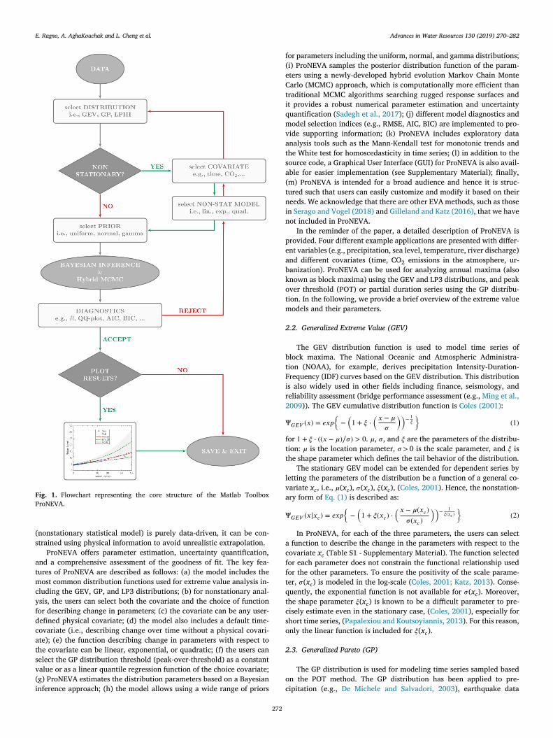
ionary extreme value analysis. Indeed, in addition to stationary EVA,roNEVA allows nonstationary analyses using user-defined covariates,hich could be time or a physical variable. Fig. 1 depicts the core struc-

ure of ProNEVA. The advantage of performing stationary analysis withhysical-related covariates resides in the possibility of imposing physicalonstraints to a statistical model. Even though such a statistical model

E. Ragno, A. AghaKouchak and L. Cheng et al. Advances in Water Resources 130 (2019) 270–282

Fig. 1. Flowchart representing the core structure of the Matlab Toolbox

ProNEVA.

(

s

a

t

m

c

y

f

d

c

a

t

s

v

(

i

f

(

e

C

t

i

q

m

v

a

t

s

a

(

t

n

i

n

p

e

a

b

k

o

t

m

2

b

t

F

i

r

2

Ψ

f

t

t

l

v

a

Ψ

a

c

f

f

t

q

t

c

s

o

2

o

c

nonstationary statistical model) is purely data-driven, it can be con-trained using physical information to avoid unrealistic extrapolation.

ProNEVA offers parameter estimation, uncertainty quantification,nd a comprehensive assessment of the goodness of fit. The key fea-ures of ProNEVA are described as follows: (a) the model includes theost common distribution functions used for extreme value analysis in-

luding the GEV, GP, and LP3 distributions; (b) for nonstationary anal-sis, the users can select both the covariate and the choice of functionor describing change in parameters; (c) the covariate can be any user-efined physical covariate; (d) the model also includes a default time-ovariate (i.e., describing change over time without a physical covari-te); (e) the function describing change in parameters with respect tohe covariate can be linear, exponential, or quadratic; (f) the users canelect the GP distribution threshold (peak-over-threshold) as a constantalue or as a linear quantile regression function of the choice covariate;g) ProNEVA estimates the distribution parameters based on a Bayesiannference approach; (h) the model allows using a wide range of priors

272

or parameters including the uniform, normal, and gamma distributions;i) ProNEVA samples the posterior distribution function of the param-ters using a newly-developed hybrid evolution Markov Chain Montearlo (MCMC) approach, which is computationally more efficient thanraditional MCMC algorithms searching rugged response surfaces andt provides a robust numerical parameter estimation and uncertaintyuantification ( Sadegh et al., 2017 ); (j) different model diagnostics andodel selection indices (e.g., RMSE, AIC, BIC) are implemented to pro-

ide supporting information; (k) ProNEVA includes exploratory datanalysis tools such as the Mann-Kendall test for monotonic trends andhe White test for homoscedasticity in time series; (l) in addition to theource code, a Graphical User Interface (GUI) for ProNEVA is also avail-ble for easier implementation (see Supplementary Material); finally,m) ProNEVA is intended for a broad audience and hence it is struc-ured such that users can easily customize and modify it based on theireeds. We acknowledge that there are other EVA methods, such as thosen Serago and Vogel (2018) and Gilleland and Katz (2016) , that we haveot included in ProNEVA.

In the reminder of the paper, a detailed description of ProNEVA isrovided. Four different example applications are presented with differ-nt variables (e.g., precipitation, sea level, temperature, river discharge)nd different covariates (time, CO 2 emissions in the atmosphere, ur-anization). ProNEVA can be used for analyzing annual maxima (alsonown as block maxima) using the GEV and LP3 distributions, and peakver threshold (POT) or partial duration series using the GP distribu-ion. In the following, we provide a brief overview of the extreme valueodels and their parameters.

.2. Generalized Extreme Value (GEV)

The GEV distribution function is used to model time series oflock maxima. The National Oceanic and Atmospheric Administra-ion (NOAA), for example, derives precipitation Intensity-Duration-requency (IDF) curves based on the GEV distribution. This distributions also widely used in other fields including finance, seismology, andeliability assessment (bridge performance assessment (e.g., Ming et al.,009 )). The GEV cumulative distribution function is Coles (2001) :

𝐺𝐸𝑉 ( 𝑥 ) = 𝑒𝑥𝑝

{

−

(1 + 𝜉 ⋅

(𝑥 − 𝜇

𝜎

))− 1

𝜉

}

(1)

or 1 + 𝜉 ⋅ ( ( 𝑥 − 𝜇) ∕ 𝜎) > 0 . 𝜇, 𝜎, and 𝜉 are the parameters of the distribu-ion: 𝜇 is the location parameter, 𝜎 > 0 is the scale parameter, and 𝜉 ishe shape parameter which defines the tail behavior of the distribution.

The stationary GEV model can be extended for dependent series byetting the parameters of the distribution be a function of a general co-ariate x c , i.e., 𝜇( x c ), 𝜎( x c ), 𝜉( x c ), ( Coles, 2001 ). Hence, the nonstation-ry form of Eq. (1) is described as:

𝐺𝐸𝑉 ( 𝑥 |𝑥 𝑐 ) = 𝑒𝑥𝑝

{

−

(1 + 𝜉( 𝑥 𝑐 ) ⋅

(𝑥 − 𝜇( 𝑥 𝑐 ) 𝜎( 𝑥 𝑐 )

))− 1 𝜉( 𝑥 𝑐 )

}

(2)

In ProNEVA, for each of the three parameters, the users can select function to describe the change in the parameters with respect to theovariate x c (Table S1 - Supplementary Material). The function selectedor each parameter does not constrain the functional relationship usedor the other parameters. To ensure the positivity of the scale parame-er, 𝜎( x c ) is modeled in the log-scale ( Coles, 2001; Katz, 2013 ). Conse-uently, the exponential function is not available for 𝜎( x c ). Moreover,he shape parameter 𝜉( x c ) is known to be a difficult parameter to pre-isely estimate even in the stationary case, ( Coles, 2001 ), especially forhort time series, ( Papalexiou and Koutsoyiannis, 2013 ). For this reason,nly the linear function is included for 𝜉( x c ).

.3. Generalized Pareto (GP)

The GP distribution is used for modeling time series sampled basedn the POT method. The GP distribution has been applied to pre-ipitation (e.g., De Michele and Salvadori, 2003 ), earthquake data

E. Ragno, A. AghaKouchak and L. Cheng et al. Advances in Water Resources 130 (2019) 270–282

(

a

o

a

e

t

Ψ

t

t

(

o

f

Ψ

W

i

e

a

t

o

m

B

𝐘

w

𝐌

n

c

o

E

𝛼

2

f

1

t

D

(

g

2

b

T

𝜓

d

t

t

𝛼

𝛽

𝜏

I

e

a

s

𝜓

3

m

E

c

p

p

T

L

S

b

𝜃

(

i

𝑝

o

p

a

o

t

d

i

p

p

M

t

i

e

(

S

d

2

B

t

p

s

b

t

4

a

d

i

d

f

q

m

I

M

N

e.g., Pisarenko and Sornette, 2003 ), wind speed ( Holmes and Mori-rty, 1999 ), and economic data (e.g., Gençay and Selçuk, 2004 ), amongthers. Given a sequence Y of independent and random variables, for large enough threshold u , the cumulative distribution function of thexcesses 𝑌 𝑒 = 𝑌 − 𝑢, conditional on Y > u , is approximated by the GP dis-ribution function, ( Coles, 2001 ):

𝐺𝑃 ( 𝑦 𝑒 ) = 1 −

(1 + 𝜉 ⋅

( 𝑦 𝑒 𝜎

))− 1

𝜉 (3)

In particular, if block maxima of Y follows a GEV distribution, thenhe threshold excesses Y e have a GP distribution in which the parame-er 𝜉 is equal to the parameter 𝜉 of the corresponding GEV distribution Coles, 2001 ).

In the nonstationary model of the GP distribution, both the thresh-ld value and the parameters of the distribution can be modeled as aunction of the user-covariate x c , ( Coles, 2001 ).

𝐺𝑃 ( 𝑦 𝑒 |𝑥 𝑐 ) = 1 −

(1 + 𝜉( 𝑥 𝑐 ) ⋅

( 𝑦 𝑒 ( 𝑥 𝑐 ) 𝜎( 𝑥 𝑐 )

))− 1 𝜉( 𝑥 𝑐 ) (4)

here 𝑌 𝑒 ( 𝑥 𝑐 ) = 𝑌 − 𝑢 ( 𝑥 𝑐 ) . Analogous to the GEV case, ProNEVA allowsncorporating different functional forms for describing change in param-ters over time or with respect to a covariate (Table S2).

The same considerations for the GEV parameter functional forms arepplied to GP distribution too. In addition, the users can specify theype of threshold u . Two quantile-based options are available: constantr linear. In the case of a linear threshold, a linear regression quantileodel is adopted. The 𝛼-regression quantile function is Koenker andassett (1978) and Kyselý et al. (2010)

= 𝐌 ⋅ 𝐔 ( 𝛼) + 𝐫 + − 𝐫 − , (5)

here 0 < 𝛼 < 1 is the quantile, �� is the column vector of n -observations, = [ 𝐗 𝐜 𝐈 𝐧 ] with X c being the column vector of covariance and I n the -identity vector, 𝐔 = [ 𝑢 1 𝑢 0 ] ′ is the vector of the regression coeffi-ients, and 𝐫 + and 𝐫 − are respectively the positive and negative partsf the residuals. Then, U( 𝜶) is calculated as the optimal solution toq. (6) ( Koenker and Bassett, 1978; Kyselý et al., 2010 ).

⋅ 𝐈 𝐧 ′ ⋅ 𝐫 + + (1 − 𝛼) ⋅ 𝐈 𝐧 ′ ⋅ 𝐫 − ∶= 𝑚𝑖𝑛 (6)

.4. Log-Pearson type III (LP3)

The LP3 distribution has been widely used in hydrology for floodrequency analysis particularly after the release of the USGS Bulletin7B ( U.S. Water Resources Council, 1982 ). However, it has been appliedo other studies, such as design magnitude of earthquakes ( Gupta andeshpande, 1994 ) and evaluation of apple bud burst time and frost risk Farajzadeh et al., 2010 ).

The LP3 distribution characterizes the random variable 𝑄 = exp ( 𝑋) ,iven that X follows a Pearson type III (P3) distribution ( Griffis et al.,007 ). Hereafter, the natural logarithm is used, however any base cane implemented, such as base-10 as in Bulletin 17B ( Griffis et al., 2007 ).he P3 probability density function is

𝑃 3 ( 𝑥 ) =

1 |𝛽| ⋅ Γ( 𝛼) ⋅ (𝑥 − 𝜏

𝛽

)𝛼−1 ⋅ exp

(−

𝑥 − 𝜏

𝛽

)(7)

efined for 𝛼 > 0, ( 𝑥 − 𝜏)∕ 𝛽 > 0 , and Γ( 𝛼) being a complete gamma func-ion ( Griffis et al., 2007 ). The parameters 𝛼, 𝛽, and 𝜏 are functions ofhe first three moments, 𝜇X , 𝜎X , 𝛾X , ( Griffis et al., 2007 ):

= 4∕ 𝛾2 𝑋

(8)

= ( 𝜎𝑋 ⋅ 𝛾𝑋 )∕2 (9)

= 𝜇𝑋 − 2 ⋅ ( 𝜎𝑋 ∕ 𝛾𝑋 ) (10)

n the case of nonstationary analysis, the first three moments are mod-led as a function of the user-defined covariate x (Table S3). The GEV

c

273

nd GP considerations mentioned above hold for the functions to de-cribe change in parameters.

𝑃 3 ( 𝑥 |𝑥 𝑐 ) =

1 |𝛽( 𝑥 𝑐 ) | ⋅ Γ( 𝛼( 𝑥 𝑐 )) ⋅(𝑥 − 𝜏( 𝑥 𝑐 )

𝛽( 𝑥 𝑐 )

)𝛼( 𝑥 𝑐 )−1 ⋅ exp

(−

𝑥 − 𝜏( 𝑥 𝑐 ) 𝛽( 𝑥 𝑐 )

)(11)

. Parameter estimation: Bayesian analysis and Markov chain

onte carlo sampling

ProNEVA estimates the parameters of the selected (non)stationaryVA distribution using a Bayesian approach, which provides a robustharacterization of the underlying uncertainty derived from both in-ut errors and model selection. Bayesian analysis has been widely im-lemented for parameter inference and uncertainty quantification (e.g.hiemann et al., 2001; Gupta et al., 2008; Cheng et al., 2014; Kwon andall, 2016; Sarhadi et al., 2016; Sadegh et al., 2017; Luke et al., 2017;adegh et al., 2018 ).

Let 𝜃 be the parameter of a given distribution and let �� = { 𝑦 1 , … , 𝑦 𝑛 }e the set of n observations. Following Bayes theorem, the probability ofgiven �� (posterior) is proportional to the product of the probability of 𝜃

prior) and the probability of �� given 𝜃 (likelihood function). Assumingndependence between the observations:

( 𝜃|�� ) ∝𝑛 ∏𝑖 =1

𝑝 ( 𝜃) ⋅ 𝑝 ( 𝑦 𝑖 |𝜃) (12)

The prior brings a priori information, which does not depend on thebserved data, into the parameter estimation process. The choice of therior distribution, then, is subjective, and it is based on prior beliefsbout the system of interest ( Sadegh et al., 2018 ). The available priorptions in ProNEVA include the uniform, normal, and gamma distribu-ions, providing a variety of possibilities. ProNEVA assumes indepen-ence of parameters and hence, each parameter requires its own prior.

In the case of a nonstationary analysis, the vector of parameters 𝜽ncludes a higher number of elements than in the stationary case, de-ending on the functional form selected for each of the distribution’sarameters.

The posterior distribution is then delineated using a hybrid-evolutionCMC approach proposed by Sadegh et al. (2017) . The MCMC simula-

ion searches for the region of interest with multiple chains runningn parallel, which share information on the fly. Moreover, the hybrid-volution MCMC benefits from an intelligent starting point selection Duan et al., 1993 ) and employs Adaptive Metropolis (AM) ( Roberts andahu, 1997; Haario et al., 1999; 2001; Roberts and Rosenthal, 2009 ),ifferential evolution (DE) ( Storn and Price, 1997; Ter Braak and Vrugt,008; Vrugt et al., 2009 ), and snooker update ( Gilks et al., 1994; Terraak and Vrugt, 2008; Sadegh and Vrugt, 2014 ) algorithms to searchhe feasible space. The Metropolis ratio is selected to accept/reject theroposed sample, and the Gelman-Rubin �� ( Gelman and Rubin, 1992 ) iselected to monitor the convergence of the chains, which should remainelow the critical threshold of 1.2. For a more detailed description ofhe algorithm, the reader is referred to Sadegh et al. (2017) .

. Model diagnostics and selection

The purpose of fitting a statistical model, whether it is station-ry or nonstationary, is to characterize the population from which theata was drawn for further analysis/inference ( Coles, 2001 ). Hence,t is necessary to check the performance of the fitted model to theata ( Coles, 2001 ). We implemented different metrics in the ProNEVAor goodness of fit (GOF) assessment and model selection including:uantile and probability plots for a graphical assessment (see Supple-entary Material), two-sample Kolmogorov-Smirnov (KS) test, Akaike

nformation Criterion (AIC), Bayesian Information Criterion (BIC),aximum Likelihood (ML), Root Mean Square Error (RMSE), andash-Sutcliff Efficiency (NSE) coefficient. The hybrid-evolution MCMC

E. Ragno, A. AghaKouchak and L. Cheng et al. Advances in Water Resources 130 (2019) 270–282

a

a

t

m

u

4

i

t

i

t

t

t

H

l

o

p

E

t

4

h

t

B

Z

a

𝐷

H

l

P

S

s

t

r

t

𝑅

4

m

V

b

r

e

(

n

e

𝐴

w

t

l

a

𝐵

w

B

4

c

a

m

𝐑

f

𝑅

𝑁

A[

5

s

s

o

a

(

𝑓

w

a

t

t

r

u

2

f

M

t

𝑓

I

a

r

v

6

fi

e

ah

c

s

cd

t

c

o

pproach ( Sadegh et al., 2017 ) within the Bayesian framework providesn ensemble of solutions for the (non)stationary statistical model fittedo the data. ProNEVA uses the best set of parameters, ��, which maxi-izes the posterior distribution. Marginal posteriors will then providencertainty estimates of the estimated parameters.

.1. Standard transformation

When applied to nonstationary applications, the lack of homogene-ty in the distributional assumption requires an adjustment to the tradi-ional GOF techniques ( Coles, 2001 ). Consequently, ProNEVA standard-zes the observations based on the underlying distribution family suchhat the GOF tests can be performed. Table S4 provides information onhe transformation methods in ProNEVA. However, it is worth notinghat the choice of the reference distribution is arbitrary ( Coles, 2001 ).ere, we selected those transformations that are widely accepted in the

iterature ( Coles, 2001; Koutrouvelis and Canavos, 1999 ). In the casef a LP3 distribution, the transformation can only be applied when thearameter 𝛼 is constant ( Koutrouvelis and Canavos, 1999 ). Based onq. (8) , this implies that the transformation can be performed only inhe case of constant skewness 𝛾X .

.2. Kolmogorov-Smirnov test

The two-sample Kolmogorov-Smirnov (KS) test is a non-parametricypothesis testing technique which compares two samples, Z (1) and Z (2) ,o assess whether they belong to the same population ( Massey, 1951 ).eing 𝐹 𝑍 (1) ( 𝑧 ) and 𝐹 𝑍 (2) ( 𝑧 ) the (unknown) statistical distributions of

(1) and Z (2) respectively, the null-hypothesis H 0 is 𝐹 𝑍 (1) ( 𝑧 ) = 𝐹 𝑍 (2) ( 𝑧 ) ,gainst alternatives. The KS test statistic D

∗ is:

∗ = max 𝑧

( |𝐹 𝑍 (1) ( 𝑧 )) − 𝐹 𝑍 (2) ( 𝑧 ) |) (13)

0 is rejected when the 𝑝 𝑣𝑎𝑙𝑢𝑒 of the test is equal to or exceeds the se-ected 𝛼-level of significance, e.g., 5%. We implemented the KS test inroNEVA as one of the methods to test the goodness-of-fit of the model.pecifically, ProNEVA generates 1000 random samples from the fittedtatistical distribution or, in the case of a nonstationary analysis, fromhe reference distribution. Then, the KS test is performed between theandom samples and the input (original or transformed) data. Finally,he rejection rate (RR), Eq. (14) , is provided as a GOF index.

𝑅 =

∑( 𝐻 0 𝑟𝑒𝑗 𝑒𝑐𝑡𝑒𝑑 )

1000 (14)

.3. Model selection based on model complexity

A model showing desirable level of performance efficiency with theinimum number of parameters, i.e., a parsimonious model ( Serago andogel, 2018 ), is usually preferred over a model with similar performanceut more parameters - e.g, a nonstationary model with more parameterselative to a simpler stationary model ( Serinaldi and Kilsby, 2015; Luket al., 2017 ). Consequently, ProNEVA evaluates different GOF metricsi.e., AIC, BIC), which account for the number of parameters within theumerical model.

The Akaike Information Criterion (AIC) ( Akaike, 1974; 1998; Ahot al., 2014 ) is formulated as follows

𝐼𝐶 = 2 ⋅ ( 𝐷 − �� ) , (15)

here D is the number of parameters of the statistical model and �� ishe log-likelihood function evaluated at ��. The model associated with aower AIC is considered a better fit.

The Bayesian Information Criterion (BIC) ( Schwarz, 1978 ) is defineds

𝐼 𝐶 = 𝐷 ⋅ 𝑙𝑛 ( 𝑁 ) − 2 ⋅ �� , (16)

here N is the length of records. Similar to AIC, the model with lowerIC results a better fit.

274

.4. Model selection based on minimum residual

Root Mean Square Error (RMSE) and Nash-Sutcliff Efficiency (NSE)oefficient are two metrics widely used in hydrology and climatologys GOF measurements ( Sadegh et al., 2018 ). The focus of both is toinimize the residuals. The vector of residual is defined as

𝐄𝐒 =

((𝐹 −1

( 1 𝑛 + 1

)− 𝑧 (1)

), … ,

(𝐹 −1

(𝑖

𝑛 + 1

)− 𝑧 ( 𝑖 )

), … , (

𝐹 −1 (

𝑛

𝑛 + 1

)− 𝑧 ( 𝑛 )

)); (17)

ollowing the same notation used for defining the quantile plot. Hence,

𝑀𝑆 𝐸 =

√ ∑𝑛

𝑖 =1 𝑅𝐸𝑆

2 𝑖

𝑛 (18)

𝑆 𝐸 = 1 −

∑𝑛

𝑖 =1 𝑅𝐸𝑆

2 𝑖 ∑𝑛

𝑖 =1 ( 𝑧 ( 𝑖 ) − 𝑚𝑒𝑎𝑛 ( 𝑧 )) 2 (19)

perfect fit is associated with RMSE = 0 and NSE = 1, given RMSE ∈0 , inf ) and NSE ∈ [− inf , 1) .

. Predictive distribution

The primary objective of a statistical inference is to predict unob-erved events ( Renard et al., 2013 ). EVA, for example, provides the ba-is for estimating loads for infrastructure design and risk assessmentf natural hazards (e.g., floods, extreme rainfall events). Considering Bayesian viewpoint, the predictive distribution can be written as Renard et al., 2013 ):

( 𝐳|�� ) = ∫ 𝑓 ( 𝐳, 𝜃|�� ) ⋅ 𝑑𝜃 = ∫ 𝑓 ( 𝐳|𝜃) ⋅ 𝑓 ( 𝜃|�� ) ⋅ 𝑑𝜃 (20)

here �� is the observed data, z is a grid at which 𝑓 ( 𝐳|�� ) will be evalu-ted, 𝜽 is the vector of parameters, f ( z | 𝜽) is the probability density func-ion (pdf) of the selected distribution (i.e., GEV, GP, LP3), and 𝑓 ( 𝜃|�� ) ishe posterior distribution function. The predictive distribution functionelies on the fitted distribution function over the parameter space, andses the posterior distribution for uncertainty estimation ( Renard et al.,013 ). In practice, Eq. (20) often cannot be derived analytically. There-ore, Renard et al. (2013) suggest to numerically evaluate it using theCMC-derived ensemble of solutions sampled from the posterior dis-

ribution. The probability density of the k th -element of the vector z is:

( 𝑧 𝑘 |�� ) =

1 𝑁 𝑠𝑖𝑚

⋅𝑁 𝑠𝑖𝑚 ∑𝑖 =1

𝑓 ( 𝑧 𝑘 |𝜃𝑖 ) (21)

n the nonstationary case, the predictive pdf is a function of the covari-te, since the distribution parameters depend on the covariates. For thiseason, ProNEVA provides the predictive pdf for a number of predefinedalues of the covariates.

. Return level curves under nonstationarity

Given a time series of annual maxima, the Return Level (RL) is de-ned as the quantile Q i for which the probability of an annual maximumxceeding the selected quantile is q i ( Cooley, 2013 ). For example, let’sssume that annual maxima of precipitation intensities 𝑃 = 𝑝 1 , … , 𝑝 𝑛 ave probability distribution F P . The quantile Q i is the value of pre-ipitation intensity such that 𝑃 𝑟 ( 𝑃 ≥ 𝑄 𝑖 ) = 1 − 𝐹 𝑃 ( 𝑄 𝑖 ) = 𝑞 𝑖 . Under thetationary assumption, the characteristics of the statistical model areonstant over time, meaning that the probability q i of the quantile Q i

oes not change on a yearly basis. In this context, the concept of Re-urn Period (RP) of the quantile Q i is defined as the inverse of its ex-eedance probability, 𝑇 𝑖 = 1∕ 𝑞 𝑖 in years. Referring back to the examplef annual maxima of precipitation intensities P , let’s assume that Q is

i

E. Ragno, A. AghaKouchak and L. Cheng et al. Advances in Water Resources 130 (2019) 270–282

t

c

R

a

(

p

(

R

i

i

o

t

e

e

(

6

e

f

s

t

(

w

6

e

w

O

c

a

t

q

𝜃

a

𝑓

w

r

𝐹

w

a

f

𝑇

C

𝑇

w

c

O

7

i

t

r

f

w

t

o

r

t

t

8

(

t

t

9

p

d

a

r

l

a

d

I

s

(

t

c

s

e

a

r

u

(

t

c

F

fi

o

a

s

t

me

s

i

c

c

w

i

9

d

u

w

he precipitation intensity quantile such that the probability of being ex-eeded in each given year is 𝑃 𝑟 ( 𝑃 ≥ 𝑄 𝑖 ) = 1 − 𝐹 𝑃 ( 𝑄 𝑖 ) = 0 . 01 . Then, theP of Q i (or RL) is 𝑇 𝑖 = 1∕ 𝑞 𝑖 = 1∕0 . 01 = 100 in years. Under the station-ry assumption, there is a one-to-one relationship between RL and RP Cooley, 2013 ). Therefore, the RL curves are defined by the followingoints:

( 𝑇 𝑖 ; 𝑄 𝑖 ) , 𝑇 𝑖 > 1 𝑦𝑟, 𝑖 = 1 , …) (22)

L curves are traditionally used for defining extreme design loads fornfrastructure design and risk assessment of natural hazards. However,n a nonstationary context both RP and RL terms become ambigu-us ( Cooley, 2013 ) and numerous studies have attempted to addresshe issue. For nonstationary analysis, ProNEVA integrates two differ-nt proposed concepts: the expected waiting time ( Salas and Obeysek-ra, 2014 ), for default time-covariate only, and the effective RL curves Katz et al., 2002 ).

.1. Effective return level

Katz et al. (2002) proposed the concept of effective design value (orffective return level), which is defined as q -quantile, Q , varying as aunction of a given covariate (i.e, time or physical). Therefore, for a con-tant value of 𝑅𝑃 = 1∕ 𝑞, where q is the yearly exceedance probability,he effective RL curves is defined by the points

( 𝑥 𝑐 , 𝑄 𝑞 ( 𝑥 𝑐 )) , 𝑞 ∈ [0 , 1]) (23)

here x c is the covariate, and Q q ( x c ) is the q -quantile.

.2. Expected waiting time

Wigley (2009) first introduced the concept of waiting time, i.e., thexpected waiting time until an event of magnitude Q i is exceeded, inhich the probability of exceedance in each year, q i , changes over time.lsen et al. (1998) and, later, Salas and Obeysekera (2014) provided aomprehensive mathematical description of the suggested concept.

The event 𝑄 𝑞 0 is defined as the event with the exceedance probability

t time 𝑡 = 0 equal to q 0 . Under nonstationary conditions, at time 𝑡 = 1he probability of exceedance of 𝑄 𝑞 0

will be q 1 , at time 𝑡 = 2 , it will be 2 , and so on. Given the selected statistical model F Q with characteristics

t , 𝑞 𝑡 = 1 − 𝐹 𝑄 ( 𝑄 𝑞 0 , 𝜃𝑡 ) . Hence, the probability of the event to exceed 𝑄 𝑞 0

t time m is given by Salas and Obeysekera (2014) :

( 𝑚 ) = 𝑞 𝑚 ⋅𝑚 −1 ∏𝑡 =1

(1 − 𝑞 𝑡 ) , (24)

here 𝑓 (1) = 𝑞 1 . The cumulative distribution function (cdf) of a geomet-ical distribution ( Eq. (24) ) is:

𝑋 ( 𝑥 ) =

𝑥 ∑𝑖 =1

𝑓 ( 𝑖 ) =

𝑥 ∑𝑖 =1

𝑞 𝑖 ⋅𝑖 −1 ∏𝑡 =1

(1 − 𝑞 𝑡 ) = 1 −

𝑥 ∏𝑡 =1

(1 − 𝑞 𝑡 ) (25)

here x is the time at which the event occurs, 𝑥 = 1 , … , 𝑥 max , 𝐹 𝑋 (1) = 𝑞 1 ,

nd 𝐹 𝑋 ( 𝑥 max ) = 1 . Therefore, the expected waiting time (or RP) in whichor the first time the occurring event exceeds 𝑄 𝑞 0

can be derived as

= 𝐸 ( 𝑋 ) =

𝑥 max ∑𝑥 =1

𝑥 ⋅ 𝑓 ( 𝑥 ) =

𝑥 max ∑𝑥 =1

𝑥 ⋅ 𝑞 𝑥

𝑥 −1 ∏𝑡 =1

(1 − 𝑞 𝑡 ) (26)

ooley (2013) simplifies Eq. (26 ) as:

= 𝐸 ( 𝑋 ) = 1 +

𝑥 𝑚𝑎𝑥 ∑𝑥 =1

𝑥 ∏𝑡 =1

(1 − 𝑞 𝑡 ) (27)

hich gives the return period under nonstationary conditions, and it isonsistent with the definition of RP in the stationary case ( Salas andbeysekera, 2014 ).

275

. Explanatory analysis: Mann-Kendall and white tests

With the intention of providing explanatory data analysis, ProNEVAncludes two different tests: the Mann-Kendall (MK) monotonic trendest and the White Test (WT) for evaluating homoscedasticity in theecords. These tests can be used to decide whether to incorporate a trendunction in one or more of the model parameters or not (i.e., decidinghether to use a stationary or nonstationary model). However, these

ests are optional and are not an integral part of ProNEVA. The selectionf a stationary versus a nonstationary analysis is untied from the testsesults, but it is left to the users. For more details about the MK and WT,he readers is referred to the Supplementary Material and the referencesherein.

. ProNEVA Graphical User Interface (GUI)

The framework here presented has also a Graphical User InterfaceGUI), Fig. 2 , which we believe can promote and facilitate the applica-ion of ProNEVA. The User Manual included in the package will providehe user with all the instructions needed.

. Results

As previously discussed, the changes in extremes observed over theast years can stem from changes in different physical processes. In or-er to account for the observed changes, we need statistical tools thatre able to incorporate those variables causing variability, which can beepresented as time-covariate or a physical-based covariate. In the fol-owing, we show example applications of ProNEVA under both stationaynd nonstationary assumptions including modeling changes induced byifferent types of covariates (both temporal and process-based changes).t is important to point out that for statistical analyses, under both thetationary and nonstationary assumptions, the quality of informationi.e., length of record, representativeness of observations), is fundamen-al. Generally, the more information is available, the more confident wean be about our inferences (and also whether or not a model is repre-entative for the application in hand). However, often observations ofxtremes are limited. The issue of data quality and availability of covari-tes is also as important for nonstationary analysis. For all application,epresentativeness of the choice of model should be rigorously testedsing different goodness-of-test methods.

In the first application, we analyze discharge data from Ferson CreekSt. Charles, IL), which has experienced intense urban development overhe years. Urbanization has a direct effect on the amount of water dis-harged at the catchment outlet, since it increases impervious surfaces.or this reason, we use a process-informed nonstationary LP3 model fortting discharge data, in which the covariate is represented by percentf urbanized catchment area. The second application involves temper-ture maxima data averaged over the Contiguous United States. Manytudies have shown that the amount of CO 2 in the atmosphere causesemperatures to increase. For this reason, we fit a nonstationary GEVodel to temperature data, in which the covariate is represented by CO 2

missions in the atmosphere to include the underlying physical relation-hip. In the third application, we investigate sea level annual maximan the city of Trieste (Italy), which has increased over the years. In thisase, we adopted a temporal nonstationary GEV model. The last appli-ation involves precipitation data for New Orleans, Louisiana, in whiche fit a stationary GP model, given that there is no evidence of change

n statistics of extremes.

.1. Application 1: Modeling discharge with urbanization as the physical

river

Since 1980, Ferson Creek (St. Charles, IL) basin has experienced landse land cover changes due to urbanization. The percent of urban areasithin the catchment has increased from 20% of the total basin’s area in

E. Ragno, A. AghaKouchak and L. Cheng et al. Advances in Water Resources 130 (2019) 270–282

Fig. 2. ProNEVA Graphical User Inter-

face (GUI). (1) Interface for uploading

data and selecting the choice of distribu-

tion (GEV/GP/LP3) and model (station-

ary/nonstationary) type; (2) Interface specific

to the choice of distribution for selecting

priors and nonstationarity model; (3) Interface

for selecting MCMC information and addi-

tional operations (e.g., additional exploratory

analyses, saving results, plotting options).

Fig. 3. Application 1: Modeling discharge in Ferson Creek with urbanization as the physical driver of change. (a) Discharge data and percent of urbanization in the

basin; (b) Discharge data as a function of urbanization.

1

u

d

p

t

o

n

u

U

i

W

o

u

t

i

(

W

a

n

s

w

s

c

t

v

a

o

t

c

c

w

o

s

m

r

u

s

9

c

s

e

a

a

a

a

p

i

r

980 to almost 65% in 2010. River discharge highly depends on the landse and land cover of the basin as it determines the ratio of infiltration toirect runoff ( Fig. 3 ). Here, urbanization can be considered as a knownhysical process that has altered the runoff in the basin. To incorporatehe known physical process, we investigate annual maxima dischargef the Ferson Creek (station USGS 05551200) using a process-informedonstationary LP3 model, in which the covariate, x c , is the percent ofrbanized area.

LP3 is widely used for modeling discharge data (Bulletin 17B,.S. Water Resources Council (1982) ). We select a nonstationary model

n which the parameter 𝜇 is an exponential function of the covariate x c .e adopt normal priors for the LP3 parameters. Fig. 4 b shows the results

f the process-informed nonstationary analysis for an arbitrary value ofrbanized area, here 37%. For the sake of comparison, Fig. 4 a displayshe results when a stationary model is implemented. It is worth not-ng that the nonstationary model ( Fig. 4 b) fits extreme discharge valueshigh values of return period) better than the stationary model ( Fig. 4 a).hile based on the AIC and BIC diagnostic tests, the stationary model

nd the nonstationary model perform rather similarly, the RMSE of theonstationary model (25.06 m

3 /s) is considerably lower than that of thetationary model (77.58 m

3 /s). Urbanization alters the runoff in the basin by reducing the amount of

ater that infiltrates and increasing the amount of direct runoff. Fig. 4 chows the ability of the statistical model to incorporate this physical pro-ess. As anticipated, the expected (ensemble median) nonstationary re-urn level curve associated with a 62% of urbanized area returns higheralues of discharge than the one associated with a 37% of urbanized

276

rea. For example, under the nonstationary assumption, the magnitudef a 50-year event is 62.47 m

3 /s for 37% of urbanized area, similar tohe stationary case. However, the magnitude of the 50-year event in-reases to 78.11 m

3 /s (25% more) for 62% of urbanized area. On theontrary, the stationary analysis estimates a 50-year event as an eventith magnitude 63.74 m

3 /s, independent of the level of urbanizationf the catchment. The result demonstrates that a combination betweentatistical concepts and physical processes is required for correctly esti-ating the expected magnitude of an event. Fig. 4 d displays the effective

eturn level curves ( Katz et al., 2002 ) which summarize the impact ofrbanization on discharge by describing return levels as functions of theelected covariate (x-axis).

.2. Application 2: Modeling temperature with CO 2 as the physical

ovariate

Over the past decades, many studies have reported increasingurface temperature (e.g.: Zhang et al., 2006; Stott et al., 2010; Melillot al., 2014; Zwiers et al., 2011 ), mainly due to anthropogenic activitiess a consequence of increase in greenhouse gasses concentration in thetmosphere. Therefore, we investigate annual maxima surface temper-ture for the Contiguous United States available from NOAA (NCDCrchive - https://www.ncdc.noaa.gov/cag/national/time-series ) using arocess-informed nonstationary GEV model in which the user-covariates represented by CO 2 emissions over the US ( Fig. 5 a). Territo-ial fossil fuel CO emissions data are available on Global Carbon

2

E. Ragno, A. AghaKouchak and L. Cheng et al. Advances in Water Resources 130 (2019) 270–282

Fig. 4. ProNEVA results for Application 1: Modeling discharge in Ferson Creek with urbanization as the physical driver of change. (a) Return Level curves based on

a stationary model; (b) Return Level base on a nonstationary model considering an urbanization area equal to 37% of the catchment area; (c) Expected return level

curves, i.e. ensemble medians, under stationary and nonstationary assumption; (d) Effective return period, i.e. return period as a function of the percent of urbanized

area.

Fig. 5. Application 2: Modeling temper-

ature maxima with CO 2 emissions as the

physical covariate. (a) Temperature and

CO 2 time series; (b) Annual temperature

maxima as a function of CO 2 emissions in

the atmosphere.

A

e

C

l

t

n

a

r

t

p

d

t

s

B

a

A

o

s

t

a

pe

s

i

o

9

s

i

f

n

P

tlas http://www.globalcarbonatlas.org/en/CO2-emissions ( Bodent al., 2017; BP, 2017; UNFCCC, 2017 ).

To incorporate the observed relationship between temperature andO 2 in the statistical model ( Fig. 5 b), we select a model in which the

ocation and the scale parameters of the GEV distribution are linear func-ions of the covariate, while the shape parameter is constant. We assumeormal priors. Fig. 6 b shows the results of the nonstationary model for value of CO 2 equal to 4.9 GtCO 2 . For comparison, we also plot theesults when a stationary model is selected in Fig. 6 a. One can see thathe nonstationary model better captures the observed extreme events,articularly events associated with higher values of CO 2 . Moreover, theiagnostics tests confirm that the nonstationary model is a better fit. Forhe nonstationary model, the AIC and the BIC are 93.91 and 104.13, re-pectively. When the stationary model is considered, both the AIC andIC increase to 104.98 and 111.11, respectively. Lower values of AICnd BIC indicate a superior model performance. The advantage of theIC and BIC for model selection is their ability to account for the numberf model parameters: models with more parameters are penalized.

277

Figure S1 shows the effective return level as a function of CO 2 emis-ions. The results show how temperature extremes change in responseo the increasing CO 2 emissions (here, the physical covariate). For ex-mple, looking at the expected magnitude of a 50-year event, the tem-erature increases of about 4%, from 18.79 ∘C to 19.5 ∘C, when the CO 2

missions increase from 4.49 GtCO 2 to 5.51 GtCO 2 . The results are con-istent with the expectation that higher CO 2 leads to a warmer climate,ndicating that the statistical nonstationary model is able to model thebserved physical relationship between temperature and CO 2 .

.3. Application 3: Modeling sea level rise with time as the covariate

The coastal city of Trieste (Italy) has been experiencing increasingea level height over the years (Fig. S2). Given the observed trend, wenvestigate annual maxima sea level data from the Permanent Serviceor Mean Sea Level (PSMSL - station ID 154) by adopting a temporalonstationary GEV model. The purpose of this example is to show thatroNEVA can also be used for temporal nonstationary analysis. The

E. Ragno, A. AghaKouchak and L. Cheng et al. Advances in Water Resources 130 (2019) 270–282

Fig. 6. ProNEVA results for Application 2:

Modeling temperature maxima with CO 2

emissions as the physical covariate. (a) Re-

turn Level curves based on a stationary

model; (b) Return Level base on a nonsta-

tionary model considering CO 2 emissions

equal to 4.9 GtCO 2 .

Fig. 7. ProNEVA results for Application 3:

Modeling sea level rise with time as the co-

variate. (a) Return Level curves based on a

stationary model; (b) Return Level base on

a nonstationary model considering equal

to 45 years from the first observation; (c)

Expected return level curves, i.e. ensemble

medians, under stationary and nonstation-

ary assumption; (d) Effective return period,

i.e. return period as a function of the co-

variate, here time.

l

l

s

c

t

F

B

t

T

t

m

f

w

T

F

8

fi

i

t

i

(

e

7

w

c

c

r

s

t

c

t

S

i

s

s

1

ocation and scale parameters of the GEV distribution are modeled asinear functions of the time-covarite. The shape parameter is kept con-tant and we use normal priors for parameter estimation.

Fig. 7 b shows the return level curves for a fixed value of the time-ovariate equal to 45 years from the first observation (i.e., 45 years intohe future from the beginning of the data). The nonstationary analysis inig. 7 b provides better performance that the stationary model in Fig. 7 a.oth the AIC and the BIC values confirm that the nonstationary model ishe best choice to represent sea level observations in a changing climate.he AIC for the nonstationary model is 976.69, while it is 992.74 forhe stationary model. Similarly, the BIC for the temporal nonstationaryodel is 989.08, while it is 1000 for the stationary model. Lower values

or AIC and BIC indicates a superior model. The value of the temporal covariate should be regarded as the time at

hich we estimate expected values of, as in this specific case, sea level.he expected (ensemble median) nonstationary return level curves inig. 7 c refer to three different time at which we evaluate sea level: 45,5, and 133 years from the first observation. Here, 133 years from therst observation is beyond the period of observations (88 years) mean-

278

ng that we project into the future the observed trend and we infer fromhere. The observed increasing trend in the sea level records results inncreasing values of sea level for higher value of the temporal covariate Fig. 7 c). For example, a 50 year event is equal to 7296.3 mm for timequal to 45 years from the first observation, 7349.3 mm for 85 years, and410.4 mm for 133 years. We register about 2% increase in sea levelhen the time of the first observation changes from 45 to 133 years,

onfirming the ability of the nonstationary model to reproduce the in-reasing trend in observations. On the contrary, the stationary analysiseturns a 50-year sea level equal to 7314.3 mm regardless of the first ob-ervation. Fig. 7 d shows the effective return level curves, which capturehe variability over time (here, the covariate) in the observed data. In thease of a nonstationary model with a temporal covariate, it is possibleo evaluate the expected waiting time ( Wigley, 2009; Olsen et al., 1998;alas and Obeysekera, 2014 ), which incorporates the observed changesn the sea level over time in the estimation of return periods. Fig. S3hows that the current return periods (lower x-axis) will change con-idering the observed nonstationarity (upper x-asis). For example, the00-year sea level estimated at t (beginning of the simulation) turns

0

E. Ragno, A. AghaKouchak and L. Cheng et al. Advances in Water Resources 130 (2019) 270–282

Fig. 8. ProNEVA results for Application 4:

Modeling precipitation under a stationary

assumption. (a) Return Level curves un-

der the stationary assumption; (b) Return

Level curves under the temporal nonsta-

tionary assumption for a value of the co-

variate within the period of observation.

i

v

9

t

a

n

c

(

s

p

a

p

p

d

e

c

r

d

t

m

t

F

h

p

p

t

1

q

a

e

m

l

f

s

t

p

f

i

a

i

w

t

N

t

d

r

i

a

e

o

s

ee

t

P

o

m

a

W

a

A

(

t

A

e

c

t

k

w

S

i

.

R

A

A

A

A

nto a 40-year event when the observed trend over time in sea levelalues is taken into account.

.4. Application 4: Modeling precipitation under a stationary assumption

This application focuses on the Generalized Pareto (GP) distribu-ion for peak-over-threshold extreme value analysis. We investigate time series of precipitation from New Orleans, Lousiana, that doesot exhibit changes in statistics of extremes. We obtain daily pre-ipitation from the National Climatic Data Center (NCDC) archive https://www.ncdc.noaa.gov/cdo-web/ ) for the city of New Orleans,tation GHCND:USW00012930. Given that we are interested in heavyrecipitation events, we use a GP distribution to focus on values above high threshold (i.e., avoid including non-extreme values). We extractrecipitation excesses considering a constant threshold of the 98th-ercentile of daily precipitation values (Fig. S4).

For this application we select a stationary GP model, given that weo not have physical evidence to justify a more complex model. How-ver, for the sake of comparison, we perform a nonstationary analysisonsidering the scale parameter as a linear function of time. Fig. 8 a rep-esents the return level curves based on a stationary model, while Fig. 8 bepicts return level curves for a value of the covariate (here time) equalo half of the period of observation. From a comparison between the twoodels, the stationary model performs better. The stationary model re-

urns values of the AIC and BIC equal to 713.3 and 721.14, respectively.or the nonstationary model the values of the AIC and BIC are slightlyigher (715.02 and 726.79, respectively). The results of this example ap-lication suggests that when no evidence of changes due to a physicalrocess can be identified, ProNEVA favors the simplest form of modelhat represents the historical observations.

0. Conclusion

The ability to reliably estimate the expected magnitude and fre-uency of extreme events is fundamental for improving design conceptsnd risk assessment methods. This is particularly important for extremevents that have significant impacts on society, infrastructure and hu-an lives, such as extreme precipitation events causing flooding and

andslides. The observed increase in extreme events and their impacts reported

rom around the world have motivated moving away from the so-calledtationary approach to ensure capturing the changing properties of ex-remes ( Milly et al., 2008 ). However, there are opposing opinions anderspective on the need and also form of suitable nonstationary modelsor extreme value analysis. Most of the existing tools for implement-ng extreme value analysis under the nonstationary assumption have number of limitations including lack of a generalized framework forncorporating physically based covariates and estimating parameters,hich depend on a generic physical covariate. To address these limi-

279

ations, we propose a generalized framework entitled Process-informed

onstationary Extreme Value Analysis (ProNEVA) in which the nonsta-ionarity component is defined by a temporal or physical-based depen-ence of the observed extremes on a physical driver (e.g., change inunoff in response to urbanization, or change in extreme temperaturesn response to CO 2 emissions). ProNEVA offers stationary and temporalnd process-informed nonstationary extreme value analysis, parameterstimation, uncertainty quantification, and a comprehensive assessmentf the goodness of fit.

Here we applied ProNEVA to four different types of applications de-cribing change in: extreme river discharge in response to urbanization,xtreme sea levels over time, extreme temperatures in response to CO 2

missions in the atmosphere. We have also demonstrated a peak-over-hreshold approach using precipitation data. The results indicate thatroNEVA offers reliable estimates when considering a physical-processr time as a covriate.

The source code of ProNEVA is freely available to the scientific com-unity. A graphical user inter face (GUI) version of the model, Fig. 2 , is

lso available to facilitate its applications (see Supporting Information).e hope that ProNEVA motivates more process-informed nonstationary

nalysis of extreme events.

cknowlgedgments

This study was partially supported by National Science FoundationNSF) grant CMMI-1635797 , National Aeronautics and Space Adminis-ration (NASA) grant NNX16AO56G , National Oceanic and Atmosphericdministration (NOAA) grant NA14OAR4310222 , and California En-rgy Commission grant 500-15-005 . The data used for the four appli-ations of the methodology proposed are freely available online. Linkso the data are provided in the dedicated section. We would like to ac-nowledge the comments of the anonymous reviewers and the Editorhich substantially improved the quality of this paper.

upplementary material

Supplementary material associated with this article can be found,n the online version, at doi: https://doi.org/10.1016/j.advwatres2019.06.007 .

eferences

ghaKouchak, A. , Feldman, D. , Stewardson, M.J. , Saphores, J.-D. , Grant, S. , Sanders, B.F. ,2014. Australia’S drought: lessons for california. Science 343 (March), 1430–1431 .

ho, K. , Derryberry, D. , Peterson, T. , 2014. Model selection for ecologists: the worldviewsof AIC and BIC. Ecology 95 (3), 631–636 .

kaike, H., 1974. A new look at the statistical model identification. IEEE Trans. Autom.Control 19 (6), 716–723. https://doi.org/10.1109/TAC.1974.1100705 .

kaike, H., 1998. Information Theory and an Extension of the Maximum Likelihood Prin-ciple BT - Selected Papers of Hirotugu Akaike. Springer New York, New York, NY,pp. 199–213. https://doi.org/10.1007/978-1-4612-1694-0_15 .

E. Ragno, A. AghaKouchak and L. Cheng et al. Advances in Water Resources 130 (2019) 270–282

A

B

B

B

B

C

C

C

C

C

C

C

C

D

D

D

F

F

F

G

G

G

G

G

G

G

G

G

H

H

H

H

H

H

H

H

J

K

K

K

KK

K

K

K

K

K

K

L

L

L

L

L

M

M

M

M

M

M

M

M

lexander, L.V., Zhang, X., Peterson, T.C., Caesar, J., Gleason, B., Klein Tank, A.M., Hay-lock, M., Collins, D., Trewin, B., Rahimzadeh, F., Tagipour, A., Rupa Kumar, K.,Revadekar, J., Griffiths, G., Vincent, L., Stephenson, D.B., Burn, J., Aguilar, E.,Brunet, M., Taylor, M., New, M., Zhai, P., Rusticucci, M., Vazquez-Aguirre, J.L., 2006.Global observed changes in daily climate extremes of temperature and precipitation.J. Geophys. Res. Atmosph. 111 (5), 1–22. https://doi.org/10.1029/2005JD006290 .

arnett, T.P., Hasselmann, K., Chelliah, M., Delworth, T., Hegerl, G., Jones, P., Rasmus-son, E., Roeckner, E., Ropelewski, C., Santer, B., Tett, S., 1999. Detection and attribu-tion of recent climate change: a status report. Bull. Am. Meteorol. Soc. 80 (12), 2631–2659. https://doi.org/10.1175/1520-0477(1999)080 < 2631:DAAORC > 2.0.CO;2 .

oden, T., Marland, G., Andres, R., 2017. Global, Regional, and National Fossil Fuel CO2Emissions. Carbon Dioxide Information Analysis Center. Oak Ridge National Labora-tory, U.S. Department of Energy, Oak Ridge, Tenn., USA. https://doi.org/10.3334/CDIAC/00001_V2017 .

P, 2017. Statistical Review of World Energy. http://www.bp.com/en/global/corporate/energy-economics.html

racken, C., Holman, K.D., Rajagopalan, B., Moradkhani, H., 2018. A Bayesian hierar-chical approach to multivariate nonstationary hydrologic frequency analysis. WaterResour. Res. 243–255. https://doi.org/10.1002/2017WR020403 .

annon, A.J., 2010. A flexible nonlinear modelling framework for nonstationary gener-alized extreme value analysis in hydroclimatology. Hydrol Process 24 (6), 673–685.https://doi.org/10.1002/hyp.7506 .

heng, L., AghaKouchak, A., 2014. Nonstationary precipitation intensity-Duration-Frequency curves for infrastructure design in a changing climate.. Sci. Rep. 4, 7093.https://doi.org/10.1038/srep07093 .

heng, L., AghaKouchak, A., Gilleland, E., Katz, R.W., 2014. Non-stationary ex-treme value analysis in a changing climate. Clim Change 127 (2), 353–369.https://doi.org/10.1007/s10584-014-1254-5 .

oles, S. , Pericchi, L. , 2003. Antecipating catastrophes through extreme value modeling.J. R. Stat. Soc. Ser. C Appl. Stat. 52 (4), 405–416 .

oles, S.G., 2001. An Introduction to Statistical Modeling of Extreme Values. Springer.https://doi.org/10.1007/978-1-4471-3675-0 .

ooley, D. , 2013. Return Periods and Return Levels Under Climate Change. SpringerNetherlands, Dordrecht, pp. 97–114 . 4

ooley, D., Nychka, D., Naveau, P., 2007. Bayesian spatial modeling of extreme precipita-tion return levels. J. Am. Stat. Assoc. 102 (479), 824–840. https://doi.org/10.1198/016214506000000780 .

oumou, D., Rahmstorf, S., 2012. A decade of weather extremes. Nat. Clim Chang. 2 (7),491–496. https://doi.org/10.1038/nclimate1452 .

e Michele, C., Salvadori, G., 2003. A generalized pareto intensity-duration modelof storm rainfall exploiting 2-Copulas. J. Geophys. Res. Atmosph. 108, 1–11.https://doi.org/10.1029/2002JD002534 .

iffenbaugh, N.S. , Swain, D.L. , Touma, D. , 2015. Anthropogenic warming has increaseddrought risk in california. Proc. Natl. Acad. Sci. 112 (13), 3931–3936 .

uan, Q.Y., Gupta, V.K., Sorooshian, S., 1993. Shuffled complex evolution approach foreffective and efficient global minimization. J. Optim. Theory Appl. 76 (3), 501–521.https://doi.org/10.1007/BF00939380 .

arajzadeh, M., Rahimi, M., Kamali, G.A., Mavrommatis, T., 2010. Modelling ap-ple tree bud burst time and frost risk in iran. Meteorol. Appl. 17 (1), 45–52.https://doi.org/10.1002/met.159 .

ischer, E.M. , Knutti, R. , 2015. Anthropogenic contribution to global occurrence of heavy–precipitation and high-temperature extremes. Nature Clim. Change 5 (6), 560–564 .

ischer, E.M., Knutti, R., 2016. Observed heavy precipitation increase confirms theoryand early models. Natl. Clim. Chang. 6 (11), 986–991. https://doi.org/10.1038/nclimate3110 .

elman, A., Rubin, D.B., 1992. Inference from iterative simulation using multiple se-quences. Stat. Sci. 7 (4), 457–472. https://doi.org/10.1214/ss/1177011136 .

ençay, R., Selçuk, F., 2004. Extreme value theory and value-at-Risk: relative performancein emerging markets. Int. J. Forecast 20 (2), 287–303. https://doi.org/10.1016/j.ijforecast.2003.09.005 .

ilks, W., Roberts, G., George, E., 1994. Adaptive direction sampling. J. R. Stat. Soc. Ser.D (Stat.) 43 (1), 179–189. https://doi.org/10.2307/2348942 .

illeland, E., Katz, R.W., 2016. extRemes 2.0: an extreme value analysis package in R. J.Stat. Softw. 72 (8). https://doi.org/10.18637/jss.v072.i08 .

illeland, E., Ribatet, M., Stephenson, A.G., 2013. A software review for extremevalue analysis. Extremes (Boston) 16 (1), 103–119. https://doi.org/10.1007/s10687-012-0155-0 . arXiv: 1011.1669v3 .

riffis, V.W. , Asce, M. , Stedinger, J.R. , Asce, M. , 2007. Log-Pearson type 3 distribution andits application in flood frequency analysis. i : distribution characteristics. J. Hydrol.Eng. 12 (October), 482–491 .

riffis, V.W., Stedinger, J.R., 2007. Incorporating Climate Change and Variability intoBulletin 17B LP3 Model. https://doi.org/10.1061/40927(243)69 .

upta, H.V., Wagener, T., Liu, Y., 2008. Reconciling theory with observations: ele-ments of a diagnostic approach to model evaluation. Hydrol Process 22, 3802–3813.https://doi.org/10.1002/hyp . November 2008

upta, I.D. , Deshpande, V.C. , 1994. Application of log-Pearson type-3 distribution forevaluation of design earthquake magnitude. J. Inst. Eng. (India), Civil Eng. Div. 75,129–134 .

aario, H., Saksman, E., Tamminen, J., 1999. Adaptive proposal distribution for randomwalk metropolis algorithm. Comput. Stat. 14 (3), 375–395. https://doi.org/10.1007/s001800050022 .

aario, H. , Saksman, E. , Tamminen, J. , 2001. An adaptive metropolis algorithm. Bernoulli7 (2), 223–242 .

aigh, I., Nicholls, R., Wells, N., 2010. Assessing changes in extreme sea levels: ap-plication to the english channel, 1900–2006. Cont. Shelf Res. 30 (9), 1042–1055.https://doi.org/10.1016/j.csr.2010.02.002 .

280

allegatte, S., Green, C., Nicholls, R.J., Corfee-Morlot, J., 2013. Future flood losses inmajor coastal cities. Nat. Clim. Chang. 3 (9), 802–806. https://doi.org/10.1038/nclimate1979 . arXiv: 1011.1669v3 .

olgate, S.J., 2007. On the decadal rates of sea level change during the twentieth century.Geophys. Res. Lett. 34 (1), 2001–2004. https://doi.org/10.1029/2006GL028492 .

olmes, J.D., Moriarty, W.W., 1999. Application of the generalized pareto distribution toextreme value analysis in wind engineering. J. Wind Eng. Ind. Aerodyn. 83 (1), 1–10.https://doi.org/10.1016/S0167-6105(99)00056-2 .

uard, D., Mailhot, A., Duchesne, S., 2009. Bayesian estimation of intensity-duration-frequency curves and of the return period associated to a given rainfallevent. Stoch. Environ. Res. Risk Ass. 24 (3), 337–347. https://doi.org/10.1007/s00477-009-0323-1 .

urkmans, R.T.W.L., Terink, W., Uijlenhoet, R., Moors, E.J., Troch, P.A., Verburg, P.H.,2009. Effects of land use changes on streamflow generation in the rhine basin. WaterResour. Res. 45 (6), 1–15. https://doi.org/10.1029/2008WR007574 .

ongman, B., Hochrainer-Stigler, S., Feyen, L., Aerts, J.C.J.H., Mechler, R., Botzen, W.J.W.,Bouwer, L.M., Pflug, G., Rojas, R., Ward, P.J., 2014. Increasing stress ondisaster-risk finance due to large floods. Nat. Clim. Chang. 4 (4), 264–268.https://doi.org/10.1038/nclimate2124 . nclimate2124

atz, R.W., 2013. Statistical methods for nonstationary extremes. In: AghaKouchak, A.,Easterling, D., Hsu, K., Schubert, S., Sorooshian, S. (Eds.), Extremes in a Changing Cli-mate: Detection, Analysis and Uncertainty. Springer Netherlands, Dordrecht, pp. 15–37. https://doi.org/10.1007/978-94-007-4479-0_2 .

atz, R.W., Parlange, M.B., Naveau, P., 2002. Statistics of extremes in hy-drology. Adv. Water Resour. 25 (8–12), 1287–1304. https://doi.org/10.1016/S0309-1708(02)00056-8 .

leme š , V., 1974. The hurst phenomenon: a puzzle? Water Resour. Res. 10 (4), 675–688.https://doi.org/10.1029/WR010i004p00675 .

oenker, R. , Bassett, G.J. , 1978. Regression quantiles. Econometrica 46 (1), 33–50 . outrouvelis, I.A., Canavos, G.C., 1999. Estimation in the pearson type 3 distribution.

Water Resour. Res. 35 (9), 2693–2704. https://doi.org/10.1029/1999WR900174 . outsoyiannis, D., 2011. Hurst-Kolmogorov dynamics and uncertainty. J. Am. Water Re-

sour. Assoc. 47 (3), 481–495. https://doi.org/10.1111/j.1752-1688.2011.00543.x . outsoyiannis, D., Montanari, A., 2007. Statistical analysis of hydroclimatic time series:

uncertainty and insights. Water Resour. Res. 43 (5), 1–9. https://doi.org/10.1029/2006WR005592 .

outsoyiannis, D., Montanari, A., 2015. Negligent killing of scientific concepts: thestationary case. Hydrol. Sci. J. 60 (7–8), 1174–1183. https://doi.org/10.1080/02626667.2014.959959 .

rishnaswamy, J., Vaidyanathan, S., Rajagopalan, B., Bonell, M., Sankaran, M.,Bhalla, R.S., Badiger, S., 2015. Non-stationary and non-linear influence of ENSO andindian ocean dipole on the variability of indian monsoon rainfall and extreme rainevents. Clim. Dyn. 45 (1), 175–184. https://doi.org/10.1007/s00382-014-2288-0 .

won, H.H., Lall, U., 2016. A copula-based nonstationary frequency analysis forthe 2012–2015 drought in california. Water Resour. Res. 52 (7), 5662–5675.https://doi.org/10.1002/2016WR018959 . 2014WR016527

yselý, J., Picek, J., Beranová, R., 2010. Estimating extremes in climate change simula-tions using the peaks-over-threshold method with a non-stationary threshold. GlobPlanet Change 72 (1–2), 55–68. https://doi.org/10.1016/j.gloplacha.2010.03.006 .

ima, C.H., Lall, U., Troy, T., Devineni, N., 2016a. A hierarchical Bayesian Gev model forimproving local and regional flood quantile estimates. J. Hydrol. (Amst) 541, 816–823. https://doi.org/10.1016/j.jhydrol.2016.07.042 .

ima, C.H., Lall, U., Troy, T.J., Devineni, N., 2015. A climate informed model for non-stationary flood risk prediction: application to negro river at manaus, amazonia. J.Hydrol. (Amst) 522, 594–602. https://doi.org/10.1016/j.jhydrol.2015.01.009 .

ima, C.H.R., Kwon, H.-H., Kim, J.-Y., 2016b. A Bayesian beta distribution model for esti-mating rainfall IDF curves in a changing climate. J. Hydrol. (Amst) 540 (SupplementC), 744–756. https://doi.org/10.1016/j.jhydrol.2016.06.062 .

ins, H.F., Cohn, T.A., 2011. Stationarity: wanted dead or alive? J. Am. Water Resour.Assoc. 47 (3), 475–480. https://doi.org/10.1111/j.1752-1688.2011.00542.x .

uke, A., Vrugt, J.A., AghaKouchak, A., Matthew, R., Sanders, B.F., 2017. Pre-dicting nonstationary flood frequencies: evidence supports an updated station-arity thesis in the united states. Water Resour. Res. 53 (7), 5469–5494.https://doi.org/10.1002/2016WR019676 .

adsen, H. , Lawrence, D. , Lang, M. , Martinkova, M. , Kjeldsen, T. , 2013. A Review ofApplied Methods in Europe for Flood-frequency Analysis in a Changing Environment .

ailhot, A., Duchesne, S., Caya, D., Talbot, G., 2007. Assessment of future changein intensity-duration-frequency (IDF) curves for southern quebec using the cana-dian regional climate model (CRCM). J. Hydrol. (Amst) 347 (1–2), 197–210.https://doi.org/10.1016/j.jhydrol.2007.09.019 .

allakpour, I., Villarini, G., 2017. Analysis of changes in the magnitude, frequency, andseasonality of heavy precipitation over the contiguous USA. Theor. Appl. Climatol.130 (1–2), 345–363. https://doi.org/10.1007/s00704-016-1881-z .

arvel, K., Bonfils, C., 2013. Identifying external influences on global precipitation. Proc.Natl. Acad. Sci. 110 (48), 19301–19306. https://doi.org/10.1073/pnas.1314382110 .

assey, F.J.J., 1951. Kolmogorov-Smirnov test for goodness of fit. J. Am. Stat. Assoc. 46(253), 68–78. https://doi.org/10.1080/01621459.1951.10500769 . dfg

atalas, N.C., 1997. Stochastic hydrology in the context of climate change.https://doi.org/10.1023/A:1005374000318 .

atalas, N.C., 2012. Comment on the announced death of stationarity. J. Wa-ter Resour. Plann. Manage. 138 (4), 311–312. https://doi.org/10.1061/(ASCE)WR.1943-5452.0000215 .

azdiyasni, O., AghaKouchak, A., 2015. Substantial increase in concurrent droughtsand heatwaves in the united states. Proc. Natl. Acad. Sci. 112 (37), 11484–11489.https://doi.org/10.1073/pnas.1422945112 .

E. Ragno, A. AghaKouchak and L. Cheng et al. Advances in Water Resources 130 (2019) 270–282

M

M

M

M

M

M

M

M

M

M

O

O

P

P

R

R

R

R

R

R

S

S

S

S

S

S

S

S

S

S

S

S

S

S

S

S

S

S

T

T

T

U

U

V

V

V

V

V

V

V

W

W

W

W

W

azdiyasni, O. , Aghakouchak, A. , Davis, S.J. , Madadgar, S. , Mehran, A. , Ragno, E. ,Sadegh, M. , Sengupta, A. , Ghosh, S. , Dhanya, C.T. , Niknejad, M. , 2017. Increasingprobability of mortality during indian heat waves. Sci. Adv. 1–6 .

elillo, J.M., Richmond, T.T., Yohe, G.W., 2014. Climate change impacts in the UnitedStates. https://doi.org/10.7930/J01Z429C.On .

entaschi, L., Vousdoukas, M., Voukouvalas, E., Sartini, L., Feyen, L., Besio, G., Alfieri, L.,2016. The transformed-stationary approach: a generic and simplified methodology fornon-stationary extreme value analysis. Hydrol. Earth Syst. Sci. 20 (9), 3527–3547.https://doi.org/10.5194/hess-20-3527-2016 .

illy, P.C.D., Betancourt, J., Falkenmark, M., Hirsch, R.M., Kundzewicz, Z.W., Letten-maier, D.P., Stouffer, R.J., 2008. Stationarity is dead: whither water management?Science 319 (5863), 573–574. https://doi.org/10.1126/science.1151915 .

in, S.-K., Zhang, X., Zwiers, F.W., Hegerl, G.C., 2011. Human contribu-tion to more-intense precipitation extremes. Nature 470 (7334), 378–381.https://doi.org/10.1038/nature09763 .

ing, L., M., F.D., Sunyong, K., 2009. Bridge system performance assessment fromstructural health monitoring: a case study. J. Struct. Eng. 135 (6), 733–742.https://doi.org/10.1061/(ASCE)ST.1943-541X.0000014 .

irhosseini, G., Srivastava, P., Fang, X., 2014. Developing rainfall intensity-Duration-Frequency (IDF) curves for alabama under future climate scenarios us-ing artificial neural network (ANN). J. Hydrol. Eng. 04014022 (11), 1–10.10.1061/(ASCE)HE.1943-5584.0000962 .

irhosseini, G., Srivastava, P., Sharifi, A., 2015. Developing probability-BasedIDF curves using kernel density estimator. J. Hydrol. Eng. 20 (9). 10.1061/(ASCE)HE.1943-5584.0001160 .

ondal, A., Mujumdar, P., 2015. Modeling non-stationarity in intensity, durationand frequency of extreme rainfall over india. J. Hydrol. (Amst) 521, 217–231.https://doi.org/10.1016/j.jhydrol.2014.11.071 .

ontanari, A., Koutsoyiannis, D., 2014. Modeling and mitigating natural haz-ards: stationary is immortal!. Water Resour. Res. 50 (12), 9748–9756.https://doi.org/10.1002/2014WR016092.Received .

beysekera, J., Salas, J.D., 2013. Quantifying the uncertainty of design floods under non-Stationary conditions. J. Hydrol. Eng. 19 (7), 1438–1446. 10.1061/(ASCE)HE.1943-5584.0000931 .

lsen, J.R., Lambert, J.H., Haimes, Y.Y., 1998. Risk of extreme events undernonstationary conditions. Risk Anal. 18 (4), 497–510. https://doi.org/10.1111/j.1539-6924.1998.tb00364.x .

apalexiou, S.M., Koutsoyiannis, D., 2013. Battle of extreme value distributions : aglobal survey on extreme daily rainfall. Water Resour. Res. 49 (1), 187–201.https://doi.org/10.1029/2012WR012557 .

isarenko, V.F., Sornette, D., 2003. Characterization of the frequency of extreme earth-quake events by the generalized pareto distribution. Pure Appl. Geophys. 160 (12),2343–2364. https://doi.org/10.1007/s00024-003-2397-x .

agno, E., AghaKouchak, A., Love, C.A., Cheng, L., Vahedifard, F., Lima, C.H.R., 2018.Quantifying changes in future intensity-Duration-Frequency curves using multi-Model ensemble simulations. Water Resour. Res. 1–38. https://doi.org/10.1002/2017WR021975 .

ead, L.K., Vogel, R.M., 2015. Reliability, return periods, and risk under nonstationar-ity. Water Resour. Res. 51 (1), 6381–6398. https://doi.org/10.1002/2014WR016259 .2014WR016527

enard, B., Sun, X., Lang, M., 2013. Bayesian methods for non-stationary extreme valueanalysis. In: AghaKouchak, A., Easterling, D., Hsu, K., Schubert, S., Sorooshian, S.(Eds.), Extremes in a Changing Climate: Detection, Analysis and Uncertainty. SpringerNetherlands, Dordrecht, pp. 39–95. https://doi.org/10.1007/978-94-007-4479-0_3 .

oberts, G.O. , Rosenthal, J.S. , 2009. Examples of adaptive MCMC. J. Comput. Graph. Stat.18 (2), 349–367 .

oberts, G.O., Sahu, S.K., 1997. Updating schemes, correlation structure, blocking andparameterization for the Gibbs sampler. J. R. Stat. Soc. Ser. B (Stat. Methodol.) 59(2), 291–317. https://doi.org/10.1111/1467-9868.00070 .

osner, A., Vogel, R.M., Kirshen, P.H., 2014. A risk-based approach to flood manage-ment decisions in a nonstationary world. Water Resour. Res. 50 (3), 1928–1942.https://doi.org/10.1002/2013WR014561.Received .

adegh, M. , Moftakhari, H. , Gupta, H.V. , Ragno, E. , Mazdiyasni, O. , Sanders, B. ,Matthew, R. , AghaKouchak, A. , 2018. Multi-hazard scenarios for analysis of com-pound extreme events. Geophys. Res. Lett. .

adegh, M., Ragno, E., Aghakouchak, A., 2017. Multivariate copula analysis toolbox (mv-cat): describing dependence and underlying uncertainty using a bayesian framework.Water Resour. Res. 1–18. https://doi.org/10.1002/2016WR020242 .

adegh, M. , Vrugt, J.A. , 2014. Approximate Bayesian computation using Markov chainmonte carlo simulation: dream (abc). Water Resour. Res. 50 (8), 6767–6787 .

adegh, M., Vrugt, J.A., Xu, C., Volpi, E., 2015. The stationarity paradigm revisited: hy-pothesis testing using diagnostics, summary metrics, and DREAM(ABC). Water Re-sour. Res. 51 (11), 9207–9231. https://doi.org/10.1002/2014WR016805 .

alas, J., Obeysekera, J., Vogel, R., 2018. Techniques for assessing water infras-tructure for nonstationary extreme events: a review. Hydrol. Sci. J. 00 (00).https://doi.org/10.1080/02626667.2018.1426858 .

alas, J.D., Obeysekera, J., 2014. Revisiting the concepts of return period and riskfor nonstationary hydrologic extreme events. J. Hydrol. Eng. (March) 554–568.10.1061/(ASCE)HE.1943-5584.0000820 .

alas, J.D. , Pielke Sr, R.A. , 2003. Stochastic characteristics and modeling of hydroclimaticprocesses. In: Potter, Thomas D., Colman, Brndley R. (Eds.), Handbook of Weather,Climate, and Water: Atmospheric Chemistry, Hydrology, and Societal Impacts. JohnWiley & Sons, Inc, pp. 585–603. ISBN 0-471-21489-2 .

alas, J.D., Rajagopalan, B., Saito, L., Brown, C., 2012. Special section on climatechange and water resources: climate nonstationarity and water resources manage-

281

ment. J. Water Resour. Plann. Manage. 138 (5), 385–388. https://doi.org/10.1061/(ASCE)WR.1943-5452.0000279 .

ankarasubramanian, A., Lall, U., 2003. Flood quantiles in a changing climate: seasonalforecasts and causal relations. Water Resour. Res. 39 (5). https://doi.org/10.1029/2002WR001593 .

arhadi, A., Burn, D.H., Concepción Ausín, M., Wiper, M.P., 2016. Time-varying nonsta-tionary multivariate risk analysis using a dynamic Bayesian copula. Water Resour.Res. 52 (3), 2327–2349. https://doi.org/10.1002/2015WR018525 .

arhadi, A., Soulis, E.D., 2017. Time-varying extreme rainfall intensity-duration-frequencycurves in a changing climate. Geophys. Res. Lett. 1–10. https://doi.org/10.1002/2016GL072201 .

chwarz, G., 1978. Estimating the dimension of a model. Ann. Stat. 6 (2), 461–464.https://doi.org/10.1214/aos/1176344136 .

erago, J.M., Vogel, R.M., 2018. Parsimonious nonstationary flood frequency anal-ysis. Adv. Water Resour. 112 (November 2017), 1–16. https://doi.org/10.1016/j.advwatres.2017.11.026 .

erinaldi, F., Kilsby, C.G., 2015. Stationarity is undead: uncertainty dominates thedistribution of extremes. Adv. Water Resour. 77, 17–36. https://doi.org/10.1016/j.advwatres.2014.12.013 .

tahl, K., Hisdal, H., Hannaford, J., Tallaksen, L.M., Van Lanen, H.A., Sauquet, E., De-muth, S., Fendekova, M., Jodar, J., 2010. Streamflow trends in europe: evidence froma dataset of near-natural catchments. Hydrol. Earth Syst. Sci. 14 (12), 2367–2382.https://doi.org/10.5194/hess-14-2367-2010 .

teinschneider, S., Lall, U., 2015. A hierarchical bayesian regional model for non-stationary precipitation extremes in northern california conditioned on tropicalmoisture exports. Water Resour. Res. 51 (3), 1472–1492. https://doi.org/10.1002/2014WR016664 .

torn, R., Price, K., 1997. Differential evolution – A simple and efficient heuristic forglobal optimization over continuous spaces. J. Global Optim. 11 (4), 341–359.https://doi.org/10.1023/A:1008202821328 .

tott, P.A., Gillett, N.P., Hegerl, G.C., Karoly, D.J., Stone, D.A., Zhang, X., Zwiers, F., 2010.Detection and attribution of climate change: a regional perspective. Wiley Interdiscip.Rev. Clim. Change 1 (2), 192–211. https://doi.org/10.1002/wcc.34 .

er Braak, C.J.F., Vrugt, J.A., 2008. Differential evolution Markov chain with snookerupdater and fewer chains. Stat Comput. 18 (4), 435–446. https://doi.org/10.1007/s11222-008-9104-9 .

hiemann, M., Trosset, M., Gupta, H., Sorooshian, S., 2001. Bayesian recursive parameterestimation for hydrologic models water resources research volume 37, issue 10. WaterResour. Res. 37 (10), 2521–2535. https://doi.org/10.1029/2000WR900405 .

owler, E., Rajagopalan, B., Gilleland, E., Summers, R.S., Yates, D., Katz, R.W., 2010.Modeling hydrologic and water quality extremes in a changing climate: a sta-tistical approach based on extreme value theory. Water Resour. Res. 46 (11).https://doi.org/10.1029/2009WR008876 .

NFCCC , 2017. National Inventory Submissions. United Nations Framework Conventionon Climate Change. .

.S. Water Resources Council , 1982. Guidelines for determining flood flow frequency.Bull. 17B: Reston, Virg. Hydrol. Subcomm. Office Water Data Coord. U.S. Geol. Surv.182 .

ahedifard, F., Robinson, J.D., AghaKouchak, A., 2016. Can protracted drought under-mine the structural integrity of California’s earthen levees? J. Geotech. Geoenviron.Eng. 142 (6), 02516001. https://doi.org/10.1061/(ASCE)GT.1943-5606.0001465 .

illarini, G., Serinaldi, F., Smith, J.A., Krajewski, W.F., 2009a. On the stationarity of an-nual flood peaks in the continental united states during the 20th century. Water Re-sour. Res. 45 (8), 1–17. https://doi.org/10.1029/2008WR007645 .

illarini, G., Smith, J.A., Napolitano, F., 2010. Nonstationary modeling of a long recordof rainfall and temperature over rome. Adv. Water Resour. 33 (10), 1256–1267.https://doi.org/10.1016/j.advwatres.2010.03.013 .

illarini, G., Smith, J.A., Serinaldi, F., Bales, J., Bates, P.D., Krajewski, W.F., 2009b.Flood frequency analysis for nonstationary annual peak records in an urbandrainage basin. Adv. Water Resour. 32 (8), 1255–1266. https://doi.org/10.1016/j.advwatres.2009.05.003 .

ogel, R.M., Yaindl, C., Walter, M., 2011. Nonstationarity: flood magnification and recur-rence reduction factors in the united states. JAWRA J. Am. Water Res. Assoc. 47 (3),464–474. https://doi.org/10.1111/j.1752-1688.2011.00541.x .

olpi, E., Fiori, A., Grimaldi, S., Lombardo, F., Koutsoyiannis, D., 2015. One hundred yearsof return period: strengths and limitations. Water Resour. Res. 51 (10), 8570–8585.https://doi.org/10.1002/2015WR017820 .

rugt, J., Ter Braak, C., Diks, C., Robinson, B., Hyman, J., Hingdon, D., 2009. AcceleratingMarkov Chain Monte Carlo Simulation by Differential Evolution with Self-AdaptiveRandomized Subspace Sampling. https://doi.org/10.1515/IJNSNS.2009.10.3.273 .

ahl, T. , Jain, S. , Bender, J. , Meyers, S.D. , Luther, M.E. , 2015. Increasing risk of compoundflooding from storm surge and rainfall for major US cities. Nature Clim. Change 5 (12),1093–1097 .

ahl, T., Jensen, J., Frank, T., Haigh, I.D., 2011. Improved estimates of mean sea levelchanges in the german bight over the last 166 years. Ocean Dyn. 61 (5), 701–715.https://doi.org/10.1007/s10236-011-0383-x .

estra, S., Alexander, L.V., Zwiers, F.W., 2013. Global increasing trends in annual max-imum daily precipitation. J. Clim. 26 (11), 3904–3918. https://doi.org/10.1175/JCLI-D-12-00502.1 .

igley, T.M., 2009. The effect of changing climate on the frequency of absolute extremeevents. Clim. Change 97 (1), 67–76. https://doi.org/10.1007/s10584-009-9654-7 .

illems, P., Arnbjerg-Nielsen, K., Olsson, J., Nguyen, V.T.V., 2012. Climate change impactassessment on urban rainfall extremes and urban drainage: methods and shortcom-ings. Atmos. Res. 103, 106–118. https://doi.org/10.1016/j.atmosres.2011.04.003 .

E. Ragno, A. AghaKouchak and L. Cheng et al. Advances in Water Resources 130 (2019) 270–282

Y

Y

Z

Z

Z

Z

an, H., Sun, N., Wigmosta, M., Skaggs, R., Hou, Z., Leung, R., 2018. Next-Generationintensity-Duration-Frequency curves for hydrologic design in snow-Dominated envi-ronments. Water Resour. Res. 1–16. https://doi.org/10.1002/2017WR021290 .

ilmaz, A.G., Perera, B.J.C., 2014. Extreme rainfall nonstationarity investigation andintensity-Frequency-Duration relationship. J. Hydrol. Eng. 19 (6), 1160–1172.10.1061/(ASCE)HE.1943-5584.0000878 .

hang, X. , Zwiers, F.W. , Hegerl, G.C. , Lambert, F.H. , Gillett, N.P. , Solomon, S. , Stott, P.A. ,Nozawa, T. , 2007. Detection of human influence on twentieth-century precipitationtrends. Nature 448 (7152), 461–465 .

282

hang, X., Zwiers, F.W., Stott, P.A., 2006. Multimodel multisignal cli-mate change detection at regional scale. J. Clim. 19 (17), 4294–4307.https://doi.org/10.1175/JCLI3851.1 .

hu, J., Stone, M.C., Forsee, W., 2012. Analysis of potential impacts of climate change onintensity - Duration - Frequency (IDF) relationships for six regions in the united states.J. Water Clim. Change 3 (3), 185–196. https://doi.org/10.2166/wcc.2012.045 .

wiers, F.W., Zhang, X., Feng, Y., 2011. Anthropogenic influence on long return pe-riod daily temperature extremes at regional scales. J. Clim. 24 (3), 881–892.https://doi.org/10.1175/2010JCLI3908.1 .