Embed Size (px)
Citation preview
AMSC 664Final
Presentation:Lagrangian
Analysis of 2Dand 3D Ocean
Flows fromEulerian
Velocity Data
David Russell
Introduction
Methods
Implementation
Validation
Application
Conclusions
Timeline
References
AMSC 664 Final Presentation:Lagrangian Analysis of 2D and 3D Ocean Flows
from Eulerian Velocity Data
David RussellSecond-year Ph.D. student, Applied Math and Scientific Computing
Project Advisor: Kayo IdeDepartment of Atmospheric and Oceanic Science
Center for Scientific Computation and Mathematical ModelingEarth System Science Interdisciplinary CenterInstitute for Physical Science and Technology
May 11th, 2016

AMSC 664Final
Presentation:Lagrangian
Analysis of 2Dand 3D Ocean
Flows fromEulerian
Velocity Data
David Russell
Introduction
Methods
Implementation
Validation
Application
Conclusions
Timeline
References
Project Goals
Project goals:
Develop tools for Lagrangian (particle-based) analysis of a2D or 3D ocean flow from Eulerian (grid-based) velocitydata
Validate on a series of simple ODE systems withwell-understood dynamics
Validate against existing tools from ROMS (RegionalOcean Modeling System)
Test on a dataset from the Chesapeake Bay

AMSC 664Final
Presentation:Lagrangian
Analysis of 2Dand 3D Ocean
Flows fromEulerian
Velocity Data
David Russell
Introduction
Methods
Implementation
Validation
Application
Conclusions
Timeline
References
Introduction
Dynamics background:
Given an ODE system x = u(t, x) (u = (u, v ,w) in R3)with corresponding particle trajectories X(t,X0)
A hyperbolic equilibrium point is a point x∗ for whichu(t, x∗) ≡ 0 and all eigenvalues of the Jacobian ∂u
∂x
∣∣x=x∗
have nonzero real part
Stable manifold of x∗: {x ∈ Rn | limt→∞X(t, x) = x∗}Unstable manifold of x∗: {x ∈ Rn | limt→−∞X(t, x) = x∗}
Corresponding concept when x∗ is moving is that of adistinguished hyperbolic trajectory

AMSC 664Final
Presentation:Lagrangian
Analysis of 2Dand 3D Ocean
Flows fromEulerian
Velocity Data
David Russell
Introduction
Methods
Implementation
Validation
Application
Conclusions
Timeline
References
Introduction
Stable and unstable manifolds:
Act as boundaries between coherent structures in the flow(e.g. as rough barriers to pollutant transport in oceans)
Can be found by one of two numerical methods:finite-time Lyapunov exponents (traditional) and arclengths, also called M-function (newer)
Each of these requires a thick soup of particle trajectoriesfor calculation

AMSC 664Final
Presentation:Lagrangian
Analysis of 2Dand 3D Ocean
Flows fromEulerian
Velocity Data
David Russell
Introduction
Methods
Implementation
Validation
Application
Conclusions
Timeline
References
Introduction
Example: M-function applied to dataset from the Kuroshiocurrent, northwest Pacific Ocean [? ]:
Red fast, blue slow (on average)
Thin yellow lines: stable and unstable manifolds
AMSC 664Final
Presentation:Lagrangian
Analysis of 2Dand 3D Ocean
Flows fromEulerian
Velocity Data
David Russell
Introduction
Methods
Implementation
Validation
Application
Conclusions
Timeline
References
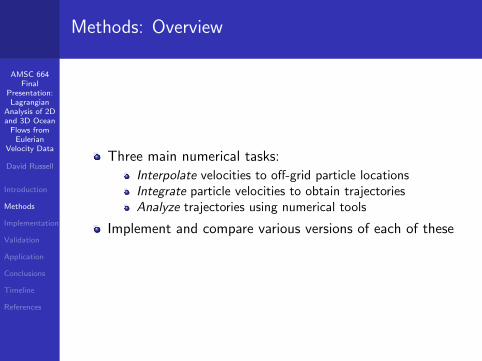
Methods: Overview
Three main numerical tasks:
Interpolate velocities to off-grid particle locationsIntegrate particle velocities to obtain trajectoriesAnalyze trajectories using numerical tools
Implement and compare various versions of each of these
AMSC 664Final
Presentation:Lagrangian
Analysis of 2Dand 3D Ocean
Flows fromEulerian
Velocity Data
David Russell
Introduction
Methods
Implementation
Validation
Application
Conclusions
Timeline
References
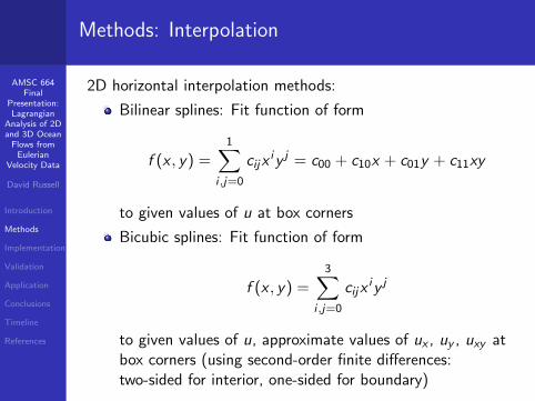
Methods: Interpolation
2D horizontal interpolation methods:
Bilinear splines: Fit function of form
f (x , y) =1∑
i ,j=0
cijxiy j = c00 + c10x + c01y + c11xy
to given values of u at box corners
Bicubic splines: Fit function of form
f (x , y) =3∑
i ,j=0
cijxiy j
to given values of u, approximate values of ux , uy , uxy atbox corners (using second-order finite differences:two-sided for interior, one-sided for boundary)

AMSC 664Final
Presentation:Lagrangian
Analysis of 2Dand 3D Ocean
Flows fromEulerian
Velocity Data
David Russell
Introduction
Methods
Implementation
Validation
Application
Conclusions
Timeline
References
Methods: Interpolation
Vertical and temporal interpolation methods:
Linear: Fit linear function of z through two nearestvertical neighbors
Cubic: Fit cubic polynomial in z through four nearestvertical neighbors
Same algorithms for temporal interpolation
Intergration method:
4th-order Runge-Kutta

AMSC 664Final
Presentation:Lagrangian
Analysis of 2Dand 3D Ocean
Flows fromEulerian
Velocity Data
David Russell
Introduction
Methods
Implementation
Validation
Application
Conclusions
Timeline
References
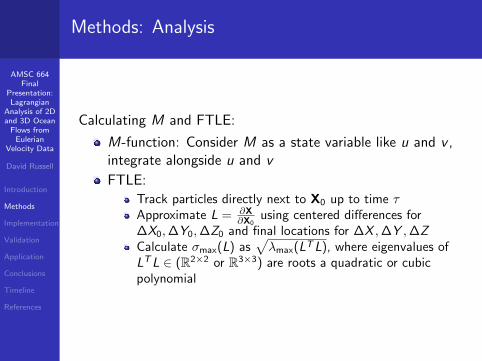
Methods: Analysis
Approaches:
M-function (arc length over fixed time interval)
Forward: M(τ,X0) =∫ τ
0|u(t,X(t,X0))| dt
Backward: M(τ,X0) =∫ 0
−τ |u(t,X(t,X0))| dtBoth: M(τ,X0) =
∫ τ−τ |u(t,X(t,X0))| dt
Maximal finite-time Lyapunov exponent (FTLE) (maximalgrowth rate of distance between close trajectories):
FTLE(τ,X0) =1
τln (σmax (L(τ,X0)))
where L(τ,X0) = ∂X(τ,X0)∂X0
is the transition matrix andσmax is the largest singular value
AMSC 664Final
Presentation:Lagrangian
Analysis of 2Dand 3D Ocean
Flows fromEulerian
Velocity Data
David Russell
Introduction
Methods
Implementation
Validation
Application
Conclusions
Timeline
References
Methods: Analysis
Calculating M and FTLE:
M-function: Consider M as a state variable like u and v ,integrate alongside u and v
FTLE:
Track particles directly next to X0 up to time τApproximate L = ∂X
∂X0using centered differences for
∆X0,∆Y0,∆Z0 and final locations for ∆X ,∆Y ,∆ZCalculate σmax(L) as
√λmax(LTL), where eigenvalues of
LTL ∈ (R2×2 or R3×3) are roots a quadratic or cubicpolynomial

AMSC 664Final
Presentation:Lagrangian
Analysis of 2Dand 3D Ocean
Flows fromEulerian
Velocity Data
David Russell
Introduction
Methods
Implementation
Validation
Application
Conclusions
Timeline
References
Implementation
Implementation details:
Software: MATLAB
Hardware:
Shorter runs (up to 6-hour dataset): MacBook Pro laptop,2.6 GHz Intel Core i5, 8 GB 1600 MHz DDR3Longer runs: Deepthought2
Vectorization but no parallelization across particles
Trajectories that leave domain set to NaN
AMSC 664Final
Presentation:Lagrangian
Analysis of 2Dand 3D Ocean
Flows fromEulerian
Velocity Data
David Russell
Introduction
Methods
Implementation
Validation
Application
Conclusions
Timeline
References
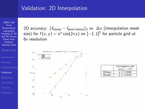
Validation: 2D Interpolation
2D accuracy: ‖finterp − fsemi-interp‖2 vs. ∆x (interpolation meshsize) for f (x , y) = ex cos(2πy) on [−1, 1]2 for particle grid at6x resolution
Convergence rate(‖e‖2 ∼ hp)
Bilinear p ≈ 2.0064Bicubic p ≈ 3.0175

AMSC 664Final
Presentation:Lagrangian
Analysis of 2Dand 3D Ocean
Flows fromEulerian
Velocity Data
David Russell
Introduction
Methods
Implementation
Validation
Application
Conclusions
Timeline
References
Validation: 3D Interpolation
3D horizontal accuracy: ‖fapprox − f ‖2 vs. ∆x = ∆y , ∆z fixed,for f (x , y , z) = ex cos 2πy cos 2πz on [−1, 1]2
Horizontal(-vertical)
method
Convergence rate(‖e‖2 ∼ hp)
Bilinear(-linear)
p ≈ 2.0253
Bicubic(-linear)
p ≈ 3.2675
Bicubic(-cubic)
p ≈ 2.9192
MATLABCubic
p ≈ 3.2675

AMSC 664Final
Presentation:Lagrangian
Analysis of 2Dand 3D Ocean
Flows fromEulerian
Velocity Data
David Russell
Introduction
Methods
Implementation
Validation
Application
Conclusions
Timeline
References
Validation: 3D Interpolation
3D vertical accuracy: ‖finterp − fsemi-interp‖2 vs. ∆z , ∆x = ∆yfixed
(Horizontal-)vertical Convergence ratemethod (‖e‖2 ∼ hp)
(Bilinear-)linear p ≈ 2.0101(Bicubic-)cubic p ≈ 4.0484MATLAB cubic p ≈ 3.2836
AMSC 664Final
Presentation:Lagrangian
Analysis of 2Dand 3D Ocean
Flows fromEulerian
Velocity Data
David Russell
Introduction
Methods
Implementation
Validation
Application
Conclusions
Timeline
References
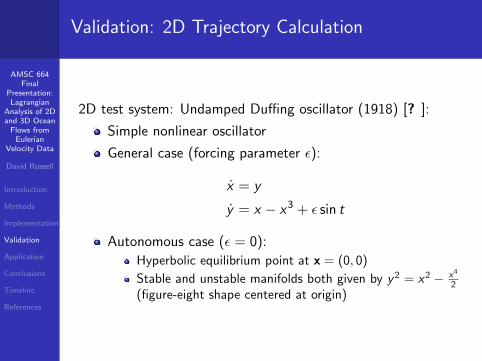
Validation: 2D Trajectory Calculation
2D test system: Undamped Duffing oscillator (1918) [? ]:
Simple nonlinear oscillator
General case (forcing parameter ε):
x = y
y = x − x3 + ε sin t
Autonomous case (ε = 0):
Hyperbolic equilibrium point at x = (0, 0)
Stable and unstable manifolds both given by y2 = x2 − x4
2(figure-eight shape centered at origin)
AMSC 664Final
Presentation:Lagrangian
Analysis of 2Dand 3D Ocean
Flows fromEulerian
Velocity Data
David Russell
Introduction
Methods
Implementation
Validation
Application
Conclusions
Timeline
References
Validation: 2D Trajectory Calculation
Autonomous Duffing oscillator:
Hamiltonian system with H(x , y) = 12y
2 − 12x
2 + 14x
4
conserved along trajectories
x(t) and y(t) can be computed explicitly via Jacobielliptic functions [? ], e.g. for y0 = 0 we have
x(t) = x0 · cn
t√
x20 − 1,
√√√√ x20
2(x20 − 1)
y(t) = −x0
√x2
0 − 1 · sn
t√
x20 − 1,
√√√√ x20
2(x20 − 1)
· dn
t√
x20 − 1,
√√√√ x20
2(x20 − 1)
AMSC 664Final
Presentation:Lagrangian
Analysis of 2Dand 3D Ocean
Flows fromEulerian
Velocity Data
David Russell
Introduction
Methods
Implementation
Validation
Application
Conclusions
Timeline
References
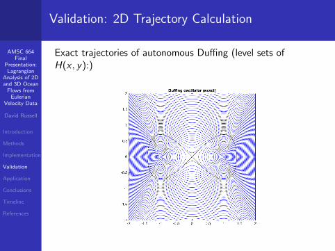
Validation: 2D Trajectory Calculation
Exact trajectories of autonomous Duffing (level sets ofH(x , y):)
AMSC 664Final
Presentation:Lagrangian
Analysis of 2Dand 3D Ocean
Flows fromEulerian
Velocity Data
David Russell
Introduction
Methods
Implementation
Validation
Application
Conclusions
Timeline
References
Validation: 2D Trajectory Calculation
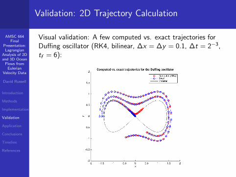
Visual validation: A few computed vs. exact trajectories forDuffing oscillator (RK4, bilinear, ∆x = ∆y = 0.1, ∆t = 2−3,tf = 6):
AMSC 664Final
Presentation:Lagrangian
Analysis of 2Dand 3D Ocean
Flows fromEulerian
Velocity Data
David Russell
Introduction
Methods
Implementation
Validation
Application
Conclusions
Timeline
References
Validation: 2D Trajectory Calculation
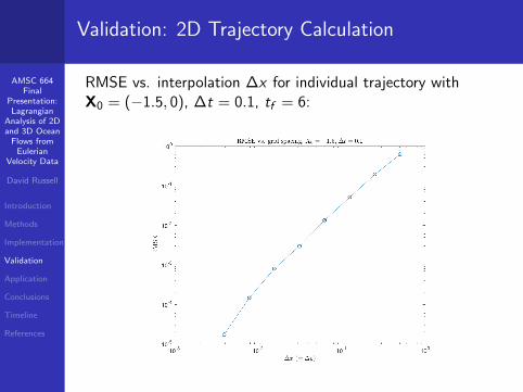
RMSE vs. interpolation ∆x for individual trajectory withX0 = (−1.5, 0), ∆t = 0.1, tf = 6:
AMSC 664Final
Presentation:Lagrangian
Analysis of 2Dand 3D Ocean
Flows fromEulerian
Velocity Data
David Russell
Introduction
Methods
Implementation
Validation
Application
Conclusions
Timeline
References
Validation: 2D Trajectory Calculation
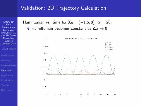
Hamiltonian vs. time for X0 = (−1.5, 0), tf = 20:
Hamiltonian becomes constant as ∆x → 0
AMSC 664Final
Presentation:Lagrangian
Analysis of 2Dand 3D Ocean
Flows fromEulerian
Velocity Data
David Russell
Introduction
Methods
Implementation
Validation
Application
Conclusions
Timeline
References
Visual Validation: 2D Lagrangian Tools
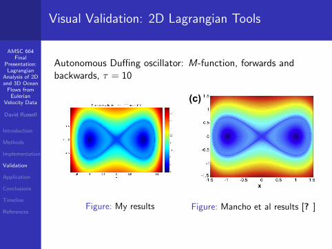
Autonomous Duffing oscillator: M-function, forwards andbackwards, τ = 10
Figure: My results
tened’’ versions of short segments of manifolds of the unstable manifold of the hyperbolic trajectory. For the longer time thecontours of the finite time average of the horizontal component of velocity develop a more complex spatial structure thatobscures the underlying unstable manifold structure of the hyperbolic trajectory.
3. Applications to time dependent 3D flows
In this section we show that Lagrangian descriptors can also provide accurate information on the stable and unstable man-ifolds of hyperbolic trajectories in three dimensional (3D) time dependent flows. Computation of the stable and unstable man-ifolds of hyperbolic trajectories in aperiodically time dependent flows was discussed in [5], where an algorithm for theircalculation was developed and several ‘‘benchmark’’ examples were considered. The particular example that we will consideris the perturbed Hill’s spherical vortex, which we will take as a benchmark for the performance of our methods in 3D. We givea brief description of the velocity field. More details on the background of Hill’s spherical vortex can be found in [5].
The velocity field, v, has the general form:
v ¼ Hðx; y; zÞ þ Sðx; y; z; tÞ
where Hðx; y; zÞ is given by:
Hx ¼ ður sin Hþ uH cos HÞ cos U; ð31ÞHy ¼ ður sin Hþ uH cos HÞ sin U; ð32ÞHz ¼ ður cos H% uH sin HÞ: ð33Þ
(a) (b) (c)
(d) (e) (f)
(g) (h) (i)
x
Fig. 13. For the integrable Duffing equation: (a) the stable and unstable manifolds of the hyperbolic fixed point; (b) forward FTLE for s ¼ 10; (c) contours ofM1 for s = 10. For the periodically forced Duffing equation: (d) segments of the stable and unstable manifolds of the hyperbolic trajectory near the origincomputed for s ¼ 10 (and displayed at t ¼ 0); (e) forward FTLE for s ¼ 10; (f) contours of M1 for s = 10. For the aperiodically forced Duffing equation: (g)segments of the stable and unstable manifolds of the hyperbolic trajectory near the origin computed for s ¼ 10 (and displayed at t ¼ 0); (h) forward FTLE fors ¼ 10; (i) contours of M1 for s = 10.
A.M. Mancho et al. / Commun Nonlinear Sci Numer Simulat 18 (2013) 3530–3557 3545
Figure: Mancho et al results [? ]

AMSC 664Final
Presentation:Lagrangian
Analysis of 2Dand 3D Ocean
Flows fromEulerian
Velocity Data
David Russell
Introduction
Methods
Implementation
Validation
Application
Conclusions
Timeline
References
Visual Validation: 2D Lagrangian Tools
Autonomous Duffing oscillator: FTLE, forwards, τ = 10
Figure: My results
tened’’ versions of short segments of manifolds of the unstable manifold of the hyperbolic trajectory. For the longer time thecontours of the finite time average of the horizontal component of velocity develop a more complex spatial structure thatobscures the underlying unstable manifold structure of the hyperbolic trajectory.
3. Applications to time dependent 3D flows
In this section we show that Lagrangian descriptors can also provide accurate information on the stable and unstable man-ifolds of hyperbolic trajectories in three dimensional (3D) time dependent flows. Computation of the stable and unstable man-ifolds of hyperbolic trajectories in aperiodically time dependent flows was discussed in [5], where an algorithm for theircalculation was developed and several ‘‘benchmark’’ examples were considered. The particular example that we will consideris the perturbed Hill’s spherical vortex, which we will take as a benchmark for the performance of our methods in 3D. We givea brief description of the velocity field. More details on the background of Hill’s spherical vortex can be found in [5].
The velocity field, v, has the general form:
v ¼ Hðx; y; zÞ þ Sðx; y; z; tÞ
where Hðx; y; zÞ is given by:
Hx ¼ ður sin Hþ uH cos HÞ cos U; ð31ÞHy ¼ ður sin Hþ uH cos HÞ sin U; ð32ÞHz ¼ ður cos H% uH sin HÞ: ð33Þ
(a) (b) (c)
(d) (e) (f)
(g) (h) (i)
x
Fig. 13. For the integrable Duffing equation: (a) the stable and unstable manifolds of the hyperbolic fixed point; (b) forward FTLE for s ¼ 10; (c) contours ofM1 for s = 10. For the periodically forced Duffing equation: (d) segments of the stable and unstable manifolds of the hyperbolic trajectory near the origincomputed for s ¼ 10 (and displayed at t ¼ 0); (e) forward FTLE for s ¼ 10; (f) contours of M1 for s = 10. For the aperiodically forced Duffing equation: (g)segments of the stable and unstable manifolds of the hyperbolic trajectory near the origin computed for s ¼ 10 (and displayed at t ¼ 0); (h) forward FTLE fors ¼ 10; (i) contours of M1 for s = 10.
A.M. Mancho et al. / Commun Nonlinear Sci Numer Simulat 18 (2013) 3530–3557 3545
Figure: Mancho et al results [? ]

AMSC 664Final
Presentation:Lagrangian
Analysis of 2Dand 3D Ocean
Flows fromEulerian
Velocity Data
David Russell
Introduction
Methods
Implementation
Validation
Application
Conclusions
Timeline
References
Visual Validation: 2D + Time Lagrangian Tools
Forced Duffing oscillator (ε = 0.1): M-function, forwards andbackwards, τ = 10
Figure: My results
tened’’ versions of short segments of manifolds of the unstable manifold of the hyperbolic trajectory. For the longer time thecontours of the finite time average of the horizontal component of velocity develop a more complex spatial structure thatobscures the underlying unstable manifold structure of the hyperbolic trajectory.
3. Applications to time dependent 3D flows
In this section we show that Lagrangian descriptors can also provide accurate information on the stable and unstable man-ifolds of hyperbolic trajectories in three dimensional (3D) time dependent flows. Computation of the stable and unstable man-ifolds of hyperbolic trajectories in aperiodically time dependent flows was discussed in [5], where an algorithm for theircalculation was developed and several ‘‘benchmark’’ examples were considered. The particular example that we will consideris the perturbed Hill’s spherical vortex, which we will take as a benchmark for the performance of our methods in 3D. We givea brief description of the velocity field. More details on the background of Hill’s spherical vortex can be found in [5].
The velocity field, v, has the general form:
v ¼ Hðx; y; zÞ þ Sðx; y; z; tÞ
where Hðx; y; zÞ is given by:
Hx ¼ ður sin Hþ uH cos HÞ cos U; ð31ÞHy ¼ ður sin Hþ uH cos HÞ sin U; ð32ÞHz ¼ ður cos H% uH sin HÞ: ð33Þ
(a) (b) (c)
(d) (e) (f)
(g) (h) (i)
x
Fig. 13. For the integrable Duffing equation: (a) the stable and unstable manifolds of the hyperbolic fixed point; (b) forward FTLE for s ¼ 10; (c) contours ofM1 for s = 10. For the periodically forced Duffing equation: (d) segments of the stable and unstable manifolds of the hyperbolic trajectory near the origincomputed for s ¼ 10 (and displayed at t ¼ 0); (e) forward FTLE for s ¼ 10; (f) contours of M1 for s = 10. For the aperiodically forced Duffing equation: (g)segments of the stable and unstable manifolds of the hyperbolic trajectory near the origin computed for s ¼ 10 (and displayed at t ¼ 0); (h) forward FTLE fors ¼ 10; (i) contours of M1 for s = 10.
A.M. Mancho et al. / Commun Nonlinear Sci Numer Simulat 18 (2013) 3530–3557 3545
Figure: Mancho et al results [? ]

AMSC 664Final
Presentation:Lagrangian
Analysis of 2Dand 3D Ocean
Flows fromEulerian
Velocity Data
David Russell
Introduction
Methods
Implementation
Validation
Application
Conclusions
Timeline
References
Visual Validation: 2D + Time Lagrangian Tools
Forced Duffing oscillator: FTLE, forwards, τ = 10
Figure: My results
tened’’ versions of short segments of manifolds of the unstable manifold of the hyperbolic trajectory. For the longer time thecontours of the finite time average of the horizontal component of velocity develop a more complex spatial structure thatobscures the underlying unstable manifold structure of the hyperbolic trajectory.
3. Applications to time dependent 3D flows
In this section we show that Lagrangian descriptors can also provide accurate information on the stable and unstable man-ifolds of hyperbolic trajectories in three dimensional (3D) time dependent flows. Computation of the stable and unstable man-ifolds of hyperbolic trajectories in aperiodically time dependent flows was discussed in [5], where an algorithm for theircalculation was developed and several ‘‘benchmark’’ examples were considered. The particular example that we will consideris the perturbed Hill’s spherical vortex, which we will take as a benchmark for the performance of our methods in 3D. We givea brief description of the velocity field. More details on the background of Hill’s spherical vortex can be found in [5].
The velocity field, v, has the general form:
v ¼ Hðx; y; zÞ þ Sðx; y; z; tÞ
where Hðx; y; zÞ is given by:
Hx ¼ ður sin Hþ uH cos HÞ cos U; ð31ÞHy ¼ ður sin Hþ uH cos HÞ sin U; ð32ÞHz ¼ ður cos H% uH sin HÞ: ð33Þ
(a) (b) (c)
(d) (e) (f)
(g) (h) (i)
x
Fig. 13. For the integrable Duffing equation: (a) the stable and unstable manifolds of the hyperbolic fixed point; (b) forward FTLE for s ¼ 10; (c) contours ofM1 for s = 10. For the periodically forced Duffing equation: (d) segments of the stable and unstable manifolds of the hyperbolic trajectory near the origincomputed for s ¼ 10 (and displayed at t ¼ 0); (e) forward FTLE for s ¼ 10; (f) contours of M1 for s = 10. For the aperiodically forced Duffing equation: (g)segments of the stable and unstable manifolds of the hyperbolic trajectory near the origin computed for s ¼ 10 (and displayed at t ¼ 0); (h) forward FTLE fors ¼ 10; (i) contours of M1 for s = 10.
A.M. Mancho et al. / Commun Nonlinear Sci Numer Simulat 18 (2013) 3530–3557 3545
Figure: Mancho et al results [? ]
AMSC 664Final
Presentation:Lagrangian
Analysis of 2Dand 3D Ocean
Flows fromEulerian
Velocity Data
David Russell
Introduction
Methods
Implementation
Validation
Application
Conclusions
Timeline
References
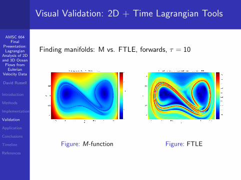
Visual Validation: 2D + Time Lagrangian Tools
Finding manifolds: M vs. FTLE, forwards, τ = 10
Figure: M-function Figure: FTLE

AMSC 664Final
Presentation:Lagrangian
Analysis of 2Dand 3D Ocean
Flows fromEulerian
Velocity Data
David Russell
Introduction
Methods
Implementation
Validation
Application
Conclusions
Timeline
References
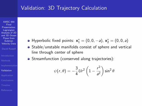
Validation: 3D Trajectory Calculation
3D test case: Hill’s spherical vortex (1894) [? ]
Simple model of axisymmetric flow around and inside asphere of radius a
Cartesian ODE system:
x = −3Uxz
2a2
y = −3Uyz
2a2
z =3U(2x2 + 2y2 + z2 − a2)
2a2
AMSC 664Final
Presentation:Lagrangian
Analysis of 2Dand 3D Ocean
Flows fromEulerian
Velocity Data
David Russell
Introduction
Methods
Implementation
Validation
Application
Conclusions
Timeline
References
Validation: 3D Trajectory Calculation
Hyperbolic fixed points: x∗1 = (0, 0,−a), x∗2 = (0, 0, a)
Stable/unstable manifolds consist of sphere and verticalline through center of sphere
Streamfunction (conserved along trajectories):
ψ(r , θ) = −3
4Ur2
(1− r2
a2
)sin2 θ

AMSC 664Final
Presentation:Lagrangian
Analysis of 2Dand 3D Ocean
Flows fromEulerian
Velocity Data
David Russell
Introduction
Methods
Implementation
Validation
Application
Conclusions
Timeline
References
Validation: 3D Trajectory Calculation
Hill’s spherical vortex: Streamfunction ψ vs. time for variousinterpolation ∆x , X0 = (0.4, 0.3, 0), ∆t = 0.1, tf = 10
ψ becomes more constant as ∆x → 0
AMSC 664Final
Presentation:Lagrangian
Analysis of 2Dand 3D Ocean
Flows fromEulerian
Velocity Data
David Russell
Introduction
Methods
Implementation
Validation
Application
Conclusions
Timeline
References
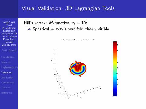
Visual Validation: 3D Lagrangian Tools
Hill’s vortex: M-function, tf = 10:
Spherical + z-axis manifold clearly visible
AMSC 664Final
Presentation:Lagrangian
Analysis of 2Dand 3D Ocean
Flows fromEulerian
Velocity Data
David Russell
Introduction
Methods
Implementation
Validation
Application
Conclusions
Timeline
References
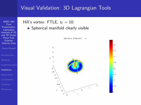
Visual Validation: 3D Lagrangian Tools
Hill’s vortex: FTLE, tf = 10:
Spherical manifold clearly visible
AMSC 664Final
Presentation:Lagrangian
Analysis of 2Dand 3D Ocean
Flows fromEulerian
Velocity Data
David Russell
Introduction
Methods
Implementation
Validation
Application
Conclusions
Timeline
References
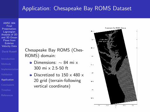
Application: Chesapeake Bay ROMS Dataset
Chesapeake Bay ROMS (Ches-ROMS) domain:
Dimensions: ∼ 84 mi x300 mi x 2.5-50 ft
Discretized to 150 x 480 x20 grid (terrain-followingvertical coordinate)

AMSC 664Final
Presentation:Lagrangian
Analysis of 2Dand 3D Ocean
Flows fromEulerian
Velocity Data
David Russell
Introduction
Methods
Implementation
Validation
Application
Conclusions
Timeline
References
Application: Chesapeake Bay ROMS Dataset
ChesROMS velocity data:
Grid indexed by (ξ, η) instead of (i , j)
Arakawa C-grid, so (ξu, ηu) staggered from (ξv , ηv )
Physical velocity components uξ, uη, vξ and vη proscribedat grid points (in m/s), also longitude (λ) and latitude (φ)
Velocity given every two minutes on spatial grid

AMSC 664Final
Presentation:Lagrangian
Analysis of 2Dand 3D Ocean
Flows fromEulerian
Velocity Data
David Russell
Introduction
Methods
Implementation
Validation
Application
Conclusions
Timeline
References
Application: Chesapeake Bay ROMS Dataset
ROMS implementation details:
Interpolation done in (ξ, η)-space (linear and bilinear only)
Velocities normalized to index space (s−1), integrationdone there
M-function calculated in physical space (m)
FTLE calculated from physical x and y displacements,estimated from λ and φ

AMSC 664Final
Presentation:Lagrangian
Analysis of 2Dand 3D Ocean
Flows fromEulerian
Velocity Data
David Russell
Introduction
Methods
Implementation
Validation
Application
Conclusions
Timeline
References
Application: Chesapeake Bay ROMS Dataset
Validating Chesapeake trajectories: Mine vs. ROMS-generated,backwards (left) and forwards (right) 60 hrs, static flow field

AMSC 664Final
Presentation:Lagrangian
Analysis of 2Dand 3D Ocean
Flows fromEulerian
Velocity Data
David Russell
Introduction
Methods
Implementation
Validation
Application
Conclusions
Timeline
References
Application: Chesapeake Bay ROMS Dataset
Trajectory error vs. time (2-norm in index space), backwardsand forwards 60 hrs

AMSC 664Final
Presentation:Lagrangian
Analysis of 2Dand 3D Ocean
Flows fromEulerian
Velocity Data
David Russell
Introduction
Methods
Implementation
Validation
Application
Conclusions
Timeline
References
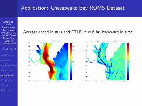
Application: Chesapeake Bay ROMS Dataset
Average speed in m/s (= Mτ ) and FTLE, τ ≈ 6 hr, forward in
time

AMSC 664Final
Presentation:Lagrangian
Analysis of 2Dand 3D Ocean
Flows fromEulerian
Velocity Data
David Russell
Introduction
Methods
Implementation
Validation
Application
Conclusions
Timeline
References
Application: Chesapeake Bay ROMS Dataset
Average speed in m/s and FTLE, τ ≈ 6 hr, forward in time

AMSC 664Final
Presentation:Lagrangian
Analysis of 2Dand 3D Ocean
Flows fromEulerian
Velocity Data
David Russell
Introduction
Methods
Implementation
Validation
Application
Conclusions
Timeline
References
Application: Chesapeake Bay ROMS Dataset
Average speed in m/s and FTLE, τ ≈ 6 hr, backward in time
AMSC 664Final
Presentation:Lagrangian
Analysis of 2Dand 3D Ocean
Flows fromEulerian
Velocity Data
David Russell
Introduction
Methods
Implementation
Validation
Application
Conclusions
Timeline
References
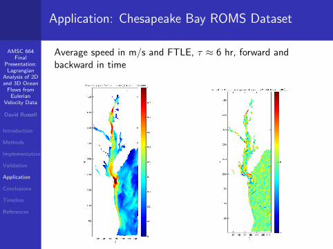
Application: Chesapeake Bay ROMS Dataset
Average speed in m/s and FTLE, τ ≈ 6 hr, forward andbackward in time

AMSC 664Final
Presentation:Lagrangian
Analysis of 2Dand 3D Ocean
Flows fromEulerian
Velocity Data
David Russell
Introduction
Methods
Implementation
Validation
Application
Conclusions
Timeline
References
Application: Chesapeake Bay ROMS Dataset
Average speed in m/s, τ ≈ 1 (left), 2 (center), and 4 (right)days, backward in time

AMSC 664Final
Presentation:Lagrangian
Analysis of 2Dand 3D Ocean
Flows fromEulerian
Velocity Data
David Russell
Introduction
Methods
Implementation
Validation
Application
Conclusions
Timeline
References
Application: Chesapeake Bay ROMS Dataset
Average speed in m/s, τ ≈ 1 (left), 2 (center), and 4 (right)days, backward in time (changing scale)

AMSC 664Final
Presentation:Lagrangian
Analysis of 2Dand 3D Ocean
Flows fromEulerian
Velocity Data
David Russell
Introduction
Methods
Implementation
Validation
Application
Conclusions
Timeline
References
Conclusions
Conclusions:
Both M-function and FTLE reveal coherent structures inan ocean flow
Boundaries of coherent structures given by large gradientsin M, ridges and troughs of FTLE
Boundary conditions important: some version of no-slip orfree-slip preferable to nothing
Interpretation somewhat sensitive to color scale, especiallyfor FTLE

AMSC 664Final
Presentation:Lagrangian
Analysis of 2Dand 3D Ocean
Flows fromEulerian
Velocity Data
David Russell
Introduction
Methods
Implementation
Validation
Application
Conclusions
Timeline
References
Timeline
October - Mid-November
Project proposal presentation and paper X2D and 3D interpolation X
Mid-November - December
2D trajectory implementation and validation XM function implementation and validation XMid-year report and presentation X
January - February
3D trajectory implementation and validation (mostly)FTLE implementation XTailor all existing code to work with ROMS data (mostly)
March - April
Apply tools to Chesapeake ROMS dataset (mostly)Final presentation and paper (in progress)

AMSC 664Final
Presentation:Lagrangian
Analysis of 2Dand 3D Ocean
Flows fromEulerian
Velocity Data
David Russell
Introduction
Methods
Implementation
Validation
Application
Conclusions
Timeline
References
References
[1] Georg Duffing. Erzwungene Schwingungen bei veranderlicherEigenfrequenz und ihre technische Bedeutung. Number 41-42. R,Vieweg & Sohn, 1918.
[2] Micaiah John Muller Hill. On a spherical vortex. Proceedings of theRoyal Society of London, 55(331-335):219–224, 1894.
[3] Ana M Mancho, Stephen Wiggins, Jezabel Curbelo, and CarolinaMendoza. Lagrangian descriptors: A method for revealing phase spacestructures of general time dependent dynamical systems.Communications in Nonlinear Science and Numerical Simulation,18(12):3530–3557, 2013.
[4] Carolina Mendoza and Ana M Mancho. Hidden geometry of oceanflows. Physical review letters, 105(3):038501, 2010.
[5] Alvaro H Salas. Exact solution to duffing equation and the pendulumequation. Applied Mathematical Sciences, 8(176):8781–8789, 2014.