Embed Size (px)
Citation preview
INTERNATIONAL JOURNAL FOR NUMERICAL METHODS IN BIOMEDICAL ENGINEERINGInt. J. Numer. Meth. Biomed. Engng. 2012; 28:52–71Published online 3 October 2011 in Wiley Online Library (wileyonlinelibrary.com). DOI: 10.1002/cnm.1468
An active strain electromechanical model for cardiac tissue
F. Nobile 1, A. Quarteroni 1,2,*,† and R. Ruiz-Baier 2
1MOX—Modellistica e Calcolo Scientifico, Dipartimento di Matematica “F. Brioschi”, Politecnico di Milano,via Bonardi 9, 20133 Milan, Italy
2Modeling and Scientific Computing, MATHICSE-SB, École Polytechnique Fédérale de Lausanne, CH-1015,Lausanne, Switzerland
SUMMARY
We propose a finite element approximation of a system of partial differential equations describing the cou-pling between the propagation of electrical potential and large deformations of the cardiac tissue. Theunderlying mathematical model is based on the active strain assumption, in which it is assumed that there is amultiplicative decomposition of the deformation tensor into a passive and active part holds, the latter carryingthe information of the electrical potential propagation and anisotropy of the cardiac tissue into the equationsof either incompressible or compressible nonlinear elasticity, governing the mechanical response of the bio-logical material. In addition, by changing from a Eulerian to a Lagrangian configuration, the bidomain ormonodomain equations modeling the evolution of the electrical propagation exhibit a nonlinear diffusionterm. Piecewise quadratic finite elements are employed to approximate the displacements field, whereas forpressure, electrical potentials and ionic variables are approximated by piecewise linear elements. Variousnumerical tests performed with a parallel finite element code illustrate that the proposed model can capturesome important features of the electromechanical coupling and show that our numerical scheme is efficientand accurate. Copyright © 2011 John Wiley & Sons, Ltd.
Received 9 May 2011; Revised 6 July 2011; Accepted 25 July 2011
KEY WORDS: cardiac electromechanical coupling; bidomain equations; reaction–diffusion problem;active strain; nonlinear elasticity; finite elements
1. INTRODUCTION
The mathematical modeling of the complex physical phenomena occurring in the heart is an areaof increasing interest, as it facilitates the better understanding of relevant mechanisms driving thebehavior of the system in both physiological and pathological contexts. In this paper, we are inter-ested in the study of the interaction between the propagation of the electrical potential through thecardiac tissue and the related mechanical response. Several difficulties and major challenges arisein this context, such as geometrical irregularities, physical nonlinearities, uncertainty of materialparameters, and anisotropy of the tissue, to name a few. This subject has gained a considerableattention in recent years, as shown by the large number of contributions in applied mathematics andbioengineering (see, e.g., [1–4] and the references therein). The diversity of these studies suggeststhat both the modeling and numerical treatment of this class of problems is far from being a resolvedsubject. A considerable amount of literature is available for the much more established understand-ing of a particular facet of the problem, namely the mechanisms that drive the electrophysiologicalactivity in the heart. From a scientific computing perspective, a wide class of numerical methodswith different degrees of complexity have been proposed and analyzed for efficiently solving the
*Correspondence to: A. Quarteroni, Modeling and Scientific Computing, MATHICSE-SB, École Polytechnique Fédéralede Lausanne, CH-1015 Lausanne, Switzerland.
†E-mail: [email protected]
Copyright © 2011 John Wiley & Sons, Ltd.
ACTIVE STRAIN IN CARDIAC ELECTROMECHANICS 53
so-called bidomain and monodomain equations modeling the propagation of electrical potentials inthe myocardium [5–8].
In this paper, we introduce some advances on a model for cardiac electromechanics, and we pro-pose a suitable numerical method for its approximation. Our model for the excitation–contractionmechanism is inspired by the description in [9,10]. The deformation of the tissue is modeled assum-ing a quasi-steady elasticity framework, in which we suppose that a multiplicative decompositionbetween the active and passive mechanical response is introduced at the deformation level. This willimply in particular that the fiber contraction driving the depolarization of the tissue rewrites in themechanical balance of forces as a prescribed active deformation, rather than as an additive contri-bution to the stresses [1]. Our proposed approach allows a direct incorporation of the micro-levelinformation on the fiber contraction in the kinematics, without the intermediate transcription of theirrole in terms of the stress. Moreover, in this context, we consider that the active part of the mechan-ical response also carries the information about the anisotropy of the fibrous tissue architecture,implying an isotropic description for the passive mechanics. Despite some necessary simplificationsin the underlying physics, the proposed model is able to address the main features of the completemechanical/electro-dynamical system, providing more insight on the role of the active strain in thecardiac electromechanical phenomenon. Our framework can of course accommodate the study ofmore general material properties, such as full orthotropy for the passive mechanical response, and awider range of model parameters.
A further aims of this paper were to devise an adequate numerical scheme for obtaining sta-ble, efficient, and accurate approximations of the underlying coupled problem and to provide somenumerical examples to illustrate the behavior of the phenomenon, which will allow us to discussthe impact of several modeling choices. The resulting nonlinear balance equations are treated usinga Newton algorithm, and the corresponding spatial discretization is performed by applying a finiteelement framework.
The remainder of this paper is organized as follows. In Section 2, the bidomain model for theelectrical activity is outlined, followed by a description of an appropriate mechanical framework onthe basis of finite elasticity. Next, we give a precise meaning to the coupling between mechanicsand electrical activity in the tissue. In Section 3, we construct the corresponding finite element for-mulation to solve the derived coupled problem, and Section 4 contains several numerical examplesthat illustrate the good behavior of the models and method proposed. Finally, some conclusions andpossible extensions are drawn in Section 5.
2. FORMULATION OF THE ELECTROMECHANICAL PROBLEM
A contraction of the cardiac muscle generally takes place in response to an electrical impulse andbecause of internal activation mechanisms. On the other hand, it is known that myocardial stretchcan cause changes in the electrophysiological properties of the heart (meccano-electrical feedback).As a matter of fact, several experimental studies both in vitro and in vivo have proved that themyocardial stretch is responsible for the change in the configuration of action potential, which leadsto afterdepolarization-like activity and arrhythmias (see, e.g., [11]).
Roughly speaking, the cardiac electromechanical response behaves as follows. An electricalimpulse starts in the sinoatrial node. There, a depolarization begins and a wave propagates across theatria, followed by a delay of the potential at the atrioventricular node. Then, a rapid depolarizationof both ventricles occurs, which at the cellular level causes an increase of calcium concentration,and this mechanism produces a contraction by a temporary binding between actin and myosin.In trying to study this complex mechanism, we will focus on the macroscopic aspects of thecoupling.
In the following, we divide the description into three main parts: the equations governing theelectrical activity, the equations for the mechanical behavior of the tissue, and finally the couplingstrategy. In order to consider each sub-problem in a natural approach, we will formulate both theelectrical propagation and the nonlinear mechanics in a pure Lagrangian framework. To this end, by�o �R3, we will denote the bounded spatial domain in the undeformed equilibrium state.
Copyright © 2011 John Wiley & Sons, Ltd. Int. J. Numer. Meth. Biomed. Engng. 2012; 28:52–71DOI: 10.1002/cnm
54 F. NOBILE, A. QUARTERONI AND R. RUIZ-BAIER
2.1. The governing equations for the electrophysiology
In this section, we recall the main equations for electrophysiology considered in a fixed mechani-cal configuration. Their extension to the case of a deforming domain is postponed to Section 2.3.The quantities of interest in the bidomain model for electrical signaling in the heart are theintracellular and extracellular electric potentials, ui D ui.x, t / and ue D ue.x, t /, defined at.x, t / 2�T WD�� .0,T /. Their difference v D v.x, t / WD ui � ue is the transmembrane potential.The conductivity of the tissue is represented by tensors Dk.x/ given by
Dk.x/D �lkal˝ alC �
tkat˝ atC �
nkan˝ an k 2 fe, ig,
where � jk 2 C
1.R3/ are intracellular and extracellular conductivities along the directions aj.x/,j 2 fl, t, ng, representing a triplet of orthonormal vectors with al.x/ being parallel to the local fibers’direction. Such description is crucial in the model, as the cardiac tissue is actually made of fibersthat drive the propagation of the electrical potential.
The bidomain model, introduced by Tung [12], is given by the following coupled reaction–diffusion system
�cm@tv �r � .Di.x/rui/C �Iion.v,w/D I iapp,
�cm@tvCr � .De.x/rue/C �Iion.v,w/D I eapp,
@tw�H.v,w/D 0, .x, t / 2�T , (2.1)
provided with homogeneous Neumann boundary conditions. Here, cm > 0 is the surface capaci-tance of the membrane, � is the ratio of membrane area per tissue volume, and w.x, t / is a ionicvariable, which essentially controls the local repolarization behavior of the action potential and itis scalar or vectorial, depending on the choice of membrane model. The symbol @t stands for thepartial derivative with respect to the time variable t . The knowledge of suitable initial conditions forv,ue,w is also required. The stimulation current possibly applied to the extracellular space is rep-resented by the functions I k
app D Ikapp.x, t /. In the case that Di D %De for some % 2R, the bidomain
system reduces to the so-called monodomain model (see, e.g., [6]):
�cm@tv �r �
�Di.x/
1C %rv
�C �Iion.v,w/D
%
1C %Iapp,
@tw�H.v,w/D 0, .x, t / 2�T . (2.2)
This somewhat simpler model requires less computational effort than (2.1), and even though theassumption of equal anisotropy ratios is physiologically inaccurate, (2.2) is still adequate for a qual-itative investigation of certain repolarization sequences and the distribution of patterns of durationsof the action potential [6].
The choice of the functions H.v,w/ and Iion.v,w/ is determined by the membrane model to beemployed. Depending on the level of complexity of the problem under investigation, we will restrictourselves to two of these. First, the adimensional Rogers–McCulloch model [13], which is basedmainly on phenomenological evidence, and corresponds to
H.v,w/D bv �w,
Iion.v,w/D c2vw � c1v.1� v/.v � a/, (2.3)
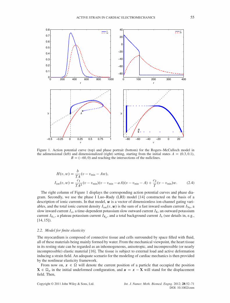
where w is a scalar gating variable, and a, b, c1, and c2 are adimensional parameters. This model isable to capture the characteristic shape of the action potential curve only on some specific repolar-ization stages (Figure 1, top). The phase diagram in Figure 1 (bottom) shows computed trajectoriesfor different initial values of v0 and w0, which converge to the stable equilibrium state .0, 0/. Inorder to provide results on a physiological scale for electrical potentials and time, we convenientlyreplaced model (2.3) by the dimensionalized equations
Copyright © 2011 John Wiley & Sons, Ltd. Int. J. Numer. Meth. Biomed. Engng. 2012; 28:52–71DOI: 10.1002/cnm
ACTIVE STRAIN IN CARDIAC ELECTROMECHANICS 55
0 200 400 600 800 10000
0.1
0.2
0.3
0.4
0.5
0.6
0.7
0.8
t
vw
0 100 200 300 400
−80
−60
−40
−20
0
20
40
t
vw
−0.5 −0.25 0 0.25 0.5 0.75 1v
w A
−80 −60 −40 −20 0 20v
w
B
Figure 1. Action potential curve (top) and phase portrait (bottom) for the Rogers–McCulloch model inthe adimensional (left) and dimensionalized (right) setting, starting from the initial states A D .0.3, 0.1/,
B D .�60, 0/ and reaching the intersections of the nullclines.
H.v,w/Db
TA.v � vmin �Aw/,
Iion.v,w/Dc1
TA2.v � vmin/.v � vmin � aA/.v � vmin �A/C
c2
T.v � vmin/w. (2.4)
The right column of Figure 1 displays the corresponding action potential curves and phase dia-gram. Secondly, we use the phase I Luo–Rudy (LRI) model [14] constructed on the basis of adescription of ionic currents. In that model, w is a vector of dimensionless ion-channel gating vari-ables, and the total ionic current density Iion.v,w/ is the sum of a fast inward sodium current INa, aslow inward current Isi, a time-dependent potassium slow outward current IK, an outward potassiumcurrent IK1 , a plateau potassium current IKp , and a total background current Ib (see details in, e.g.,[14, 15]).
2.2. Model for finite elasticity
The myocardium is composed of connective tissue and cells surrounded by space filled with fluid,all of these materials being mainly formed by water. From the mechanical viewpoint, the heart tissuein its resting state can be regarded as an inhomogeneous, anisotropic, and incompressible (or nearlyincompressible) elastic material [16]. The tissue is subject to external load and active deformationinducing a strain field. An adequate scenario for the modeling of cardiac mechanics is then providedby the nonlinear elasticity framework.
From now on, x 2 � will denote the current position of a particle that occupied the positionX 2 �o in the initial undeformed configuration, and u D x � X will stand for the displacementfield. Then,
Copyright © 2011 John Wiley & Sons, Ltd. Int. J. Numer. Meth. Biomed. Engng. 2012; 28:52–71DOI: 10.1002/cnm
56 F. NOBILE, A. QUARTERONI AND R. RUIZ-BAIER
FDrx D ICru, Fij D@xi
@XjD ıij C
@ui
@Xj,
where ıij denotes the Kronecker delta and is the deformation gradient tensor, measuring strainbetween the deformed and undeformed states. The symbol r denotes the gradient of a quantitywith respect to the material coordinates X. We assume that F can be decomposed (factorized) intoan elastic (passive) factor, taking place at a macroscale, and an active deformation gradient tensor,acting at a microscale in the following form [10]
FD FeFa. (2.5)
Such decomposition assumes that an intermediate elastic configuration �e exists between thereference state �o and the current loaded configuration �.
Notice that F is given by the gradient of a vector map whereas Fe , Fa are not, in general. In thesequel, we will refer to this setting as the active strain formulation. Similar decompositions havebeen proposed in the context of finite elastoplasticity [17] and growth modeling [18].
By J ,Ja, we denote the determinants of F, Fa, respectively. The Jacobian J describes the volumemap of infinitesimal reference elements onto the corresponding current elements. In other elec-tromechanical models available (see, e.g., [2–4, 19]), an appropriate term is added to the passivestress tensor, generating an additive decomposition between passive and active stress. We will referto the latter decomposition as active stress formulation. It is demonstrated in [10] that the activestress decomposition is equivalent to (2.5) only in the special case of small deformations.
The time–space scales in the cardiac electromechanical phenomenon suggest the use of steady-state equations of motion to describe the conservation of linear and angular momentum [3]. Theseare reduced to the force balance
�r � PD f ,
where P is the Piola–Kirchhoff stress, which represents force per unit undeformed surface, and fis a vector of body forces. Note that the balance is defined in the undeformed state �o.
The definition of P in terms of the components of the deformation stress and strain measures isgiven by the constitutive relations. In the context under study, the medium is typically assumed tobe a hyperelastic material. Therefore, it can be postulated that there exists an elastic strain energydensity function W D W.F/ defined in the reference configuration and depending only on thevalue of the deformation gradient, which characterizes the material. Notice that the energy in theintermediate elastic configuration is
We DW.Fe/DW.FF�1a /,
and therefore a pull back to the reference state gives a new energy
bW D JaW.FF�1a /.
We point out that if the chosen strain energy function has desirable stability properties (such aspolyconvexity and coercivity, as discussed in, e.g., [16]), then the application of an active straindecomposition like (2.5) essentially translates into a natural shift of the relaxation state from I toF�1a , therefore preserving the qualitative structure of W . In this sense, the active strain formulationcan be straightforwardly extended to the study of more adequate material laws, such as structurallybased models that account for the passive properties of the cardiac tissue.
For the derivation of the full model, we start by considering a Neo-Hookean material, for whichthe internal stored energy function in the intermediate configuration reads
W.Fe/D�1
2tr�FTe Fe � I
�,
where �1 is a shear modulus. To assure incompressibility of the material (where only isochoricbehavior is allowed), we assumed the strain energy to take the form
Copyright © 2011 John Wiley & Sons, Ltd. Int. J. Numer. Meth. Biomed. Engng. 2012; 28:52–71DOI: 10.1002/cnm
ACTIVE STRAIN IN CARDIAC ELECTROMECHANICS 57
bW D JaW.Fe/� p.J � 1/,
where p is the Lagrange multiplier arising from the imposition of the incompressibility constraintJ D 1 (conservation of mass) and which is usually interpreted as the hydrostatic pressure field.
The Piola–Kirchhoff stress tensor is given by the Frechet derivative of the internal stored energyfunction W , which in the fully relaxed configuration reads
PD Ja@W@Fe
F�Ta � pF�Te F�Ta .
An alternative step considered here is the assumption of nearly incompressible materials, whichin turn allows to avoid solving a saddle-point-like problem. In such case, a suitable strain energyfunction for Neo-Hookean materials is [20]
W.Fe/D�1
2Jatr.FTe Fe � I/C
�2
2.J � 1/2 ��1Ja ln.J /,
if J > 0, and W.Fe/ D 1 otherwise. Here, �2 is a bulk modulus. The discussion on whetherthe myocardium should be modeled as incompressible or nearly incompressible is apparently notresolved; we therefore leave the door open for considering both approaches.
Notice that in the material law used herein, so far we have not addressed a major feature in themodeling of cardiac dynamics: the anisotropy of the tissue. Obviously, the strain energy could alsobe assumed to depend explicitly on the fibers distribution through the inclusion of further invariantsof the left Cauchy–Green tensor or through components of the Green–Lagrange strain tensor, as in,for example, [3, 21, 22].
In this work, we follow a simplified approach and, as an intermediate step, propose to account forthe anisotropic behavior of the fibers only by assigning direction-specific active deformation fieldsin the active part of the decomposition. That is, we assume for the moment that the passive elasticresponse is isotropic. More specifically, for a myofiber distribution along the direction of the unitvectors al, at, we consider that the active strain assumes the form
Fa D IC �lal˝ alC �tat˝ at, (2.6)
where al, at are the fiber sheet longitudinal and transversal directions respectively, and �i are scalarfields accounting for the activation, depending on macroscopic stimuli related to the electrical partof the model, which will be made precise later. Given the special constitutive form of Fa, undertransverse anisotropy, we can readily write
Ja D .1C �l/.1C �t/.
Putting together the previous description, we obtain that the Euler–Lagrange problem (in its weakformulation) reads as follows: find u,p in suitable admissible displacement and pressure spacessuch that Z
�o
��1Ja.ICru/F�1a F�Ta W r'� pJ.ICru/
�T W r'�D 0 (2.7)Z
�o
.J � 1/q D 0,
for all test functions ', q in the same spaces as u and p, respectively.
2.3. The coupled model
With the purpose of studying the basic mechanisms of the meccano-electrical feedback, andthe related numerical challenges, we herein consider a coupled model in which we retain onlythe most essential elements. We first assume that the active deformation functions �j, j 2 fl, tg
Copyright © 2011 John Wiley & Sons, Ltd. Int. J. Numer. Meth. Biomed. Engng. 2012; 28:52–71DOI: 10.1002/cnm
58 F. NOBILE, A. QUARTERONI AND R. RUIZ-BAIER
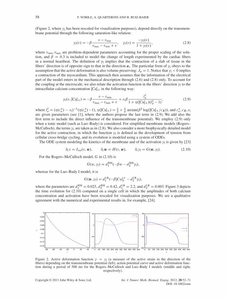
(Figure 2, where �j has been rescaled for visualization purposes), depend directly on the transmem-brane potential through the following saturation-like relation:
�l.v/D�ˇv � vmin
vmax � vminC v, �t.v/D
��l.v/
1C �l.v/, (2.8)
where vmin, vmax are problem-dependent parameters accounting for the proper scaling of the solu-tion, and ˇ D 0.3 is included to model the change of length experimented by the cardiac fibersin a normal heartbeat. The definition of �l implies that the contraction of a slab of tissue in thefibers’ direction is of opposite sign to that in the direction at. The particular form of �t obeys to theassumption that the active deformation is also volume preserving: Ja D 1. Notice that �l < 0 impliesa contraction of the myocardium. This approach then assumes that the information of the electricalpart of the model enters in the mechanical description through (2.6) and (2.8) only. To account forthe coupling at the microscale, we also relate the activation function in the fibers’ direction �l to theintracellular calcium concentration ŒCa�C in the following way:
�l.v, ŒCa�C/D�ˇv � vmin
vmax � vminC vC "lˇ
l lo
1C �.ŒCa�C/.l lo � 1/, (2.9)
where l lo D .�.c�o / � "l/
�1.�.c�o /�1/, �.ŒCa�C/D 12C 1
�arctan.ˇ2 log.ŒCa�C=cR//, and c�o , cR, "l
are given parameters (see [1], where the authors propose the last term in (2.9). We add also thefirst term to include the direct influence of the transmembrane potential). We employ (2.9) onlywhen a ionic model (such as Luo–Rudy) is considered. For simplified membrane models (Rogers–McCulloch), the terms �i are taken as in (2.8). We also consider a more biophysically detailed modelfor the active contraction, in which the function �l is defined as the development of tension fromcellular cross-bridge cycling, and its evolution is modeled using a system of ODEs.
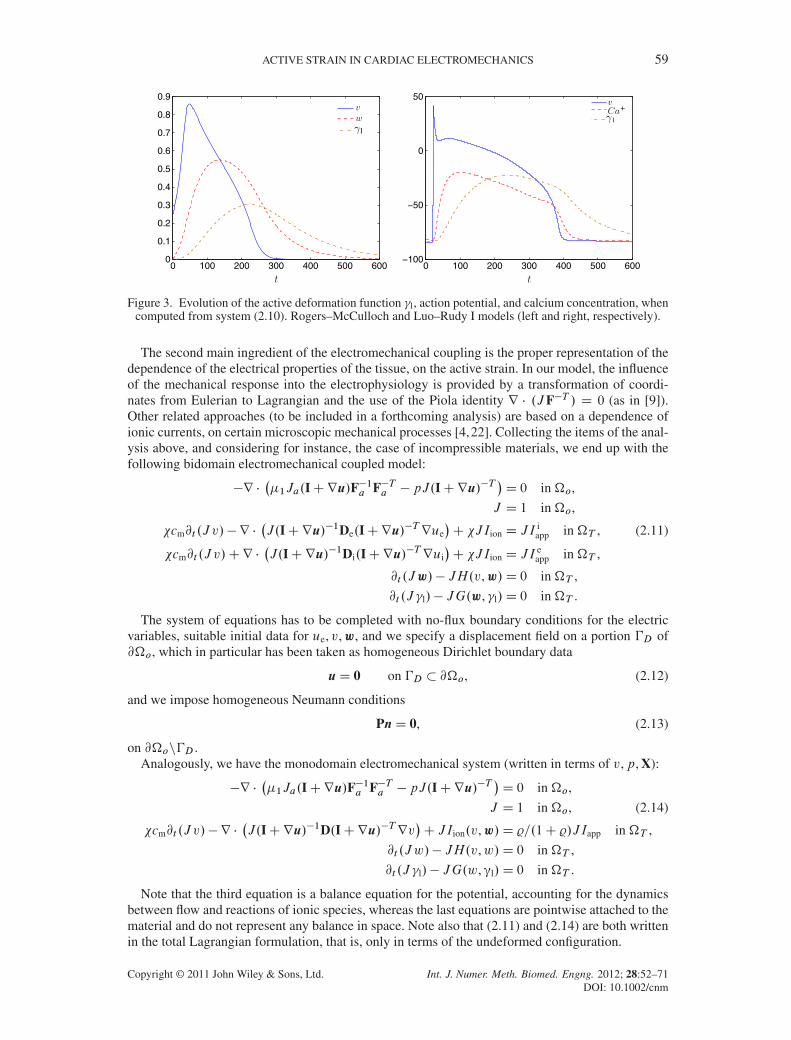
The ODE system modeling the kinetics of the membrane and of the activation �l is given by [23]
@tv D Iion.v,w/, @twDH.v,w/, @t�l DG.w, �l/. (2.10)
For the Rogers–McCulloch model, G in (2.10) is
G.w, �l/D dRM1 .�ˇw � dRM
2 �l/,
whereas for the Luo–Rudy I model, it is
G.w, �l/D dLR1 .�ˇŒCa�Ci � d
LR2 �l/,
where the parameters are dRM1 D 0.025, dRM
2 D 0.42, dLR1 D 2.2, and dLR
2 D 0.005. Figure 3 depictsthe time evolution for (2.10) computed on a single cell in which the amplitudes of both calciumconcentration and activation have been rescaled for visualization purposes. We see a qualitativeagreement with the numerical and experimental results in, for example, [24].
−80 −60 −40 −20 0 20 40
−0.16
−0.14
−0.12
−0.1
−0.08
−0.06
−0.04
−0.02
0
0 50 100 150 200 250 300 350 400 450 500−100
−50
0
50
0 50 100 150 200 250 300 350 400 450 500−100
−50
0
50
Figure 2. Active deformation function � D �l (a measure of the active strain in the direction of thefibers) depending on the transmembrane potential (left), action potential curve and active deformation func-tion during a period of 500 ms for the Rogers–McCulloch and Luo–Rudy I models (middle and right,
respectively).
Copyright © 2011 John Wiley & Sons, Ltd. Int. J. Numer. Meth. Biomed. Engng. 2012; 28:52–71DOI: 10.1002/cnm
ACTIVE STRAIN IN CARDIAC ELECTROMECHANICS 59
0 100 200 300 400 500 6000
0.1
0.2
0.3
0.4
0.5
0.6
0.7
0.8
0.9
l
0 100 200 300 400 500 600−100
−50
0
50
l
Figure 3. Evolution of the active deformation function �l, action potential, and calcium concentration, whencomputed from system (2.10). Rogers–McCulloch and Luo–Rudy I models (left and right, respectively).
The second main ingredient of the electromechanical coupling is the proper representation of thedependence of the electrical properties of the tissue, on the active strain. In our model, the influenceof the mechanical response into the electrophysiology is provided by a transformation of coordi-nates from Eulerian to Lagrangian and the use of the Piola identity r � .JF�T / D 0 (as in [9]).Other related approaches (to be included in a forthcoming analysis) are based on a dependence ofionic currents, on certain microscopic mechanical processes [4,22]. Collecting the items of the anal-ysis above, and considering for instance, the case of incompressible materials, we end up with thefollowing bidomain electromechanical coupled model:
�r ���1Ja.ICru/F�1a F�Ta � pJ.ICru/
�T�D 0 in�o,
J D 1 in�o,
�cm@t .J v/�r ��J.ICru/�1De.ICru/�True
�C �JIion D JI
iapp in�T , (2.11)
�cm@t .J v/Cr ��J.ICru/�1Di.ICru/�Trui
�C �JIion D JI
eapp in�T ,
@t .Jw/� JH.v,w/D 0 in�T ,
@t .J �l/� JG.w, �l/D 0 in�T .
The system of equations has to be completed with no-flux boundary conditions for the electricvariables, suitable initial data for ue, v,w, and we specify a displacement field on a portion D of@�o, which in particular has been taken as homogeneous Dirichlet boundary data
uD 0 on D � @�o, (2.12)
and we impose homogeneous Neumann conditions
PnD 0, (2.13)
on @�onD .Analogously, we have the monodomain electromechanical system (written in terms of v,p, X):
�r ���1Ja.ICru/F�1a F�Ta � pJ.ICru/
�T�D 0 in�o,
J D 1 in�o, (2.14)
�cm@t .J v/�r ��J.ICru/�1D.ICru/�Trv
�C JIion.v,w/D %=.1C %/JIapp in�T ,
@t .Jw/� JH.v,w/D 0 in�T ,
@t .J �l/� JG.w, ”l/D 0 in�T .
Note that the third equation is a balance equation for the potential, accounting for the dynamicsbetween flow and reactions of ionic species, whereas the last equations are pointwise attached to thematerial and do not represent any balance in space. Note also that (2.11) and (2.14) are both writtenin the total Lagrangian formulation, that is, only in terms of the undeformed configuration.
Copyright © 2011 John Wiley & Sons, Ltd. Int. J. Numer. Meth. Biomed. Engng. 2012; 28:52–71DOI: 10.1002/cnm
60 F. NOBILE, A. QUARTERONI AND R. RUIZ-BAIER
2.4. Weak formulation
Let us denote H 1D.�o/ D fs 2 H
1.�o/ W sj�D D 0g. Assuming that all unknowns are regularenough (we suppose v,ue 2 L
2.0,T IH 1.�o//, w 2 L2.0,T ,L2.�o//, u 2 L2.0,T IH 1D.�o/
3/,p 2 L20.�o/, in order to get bounded energy integrals), we multiply the equations in (2.11) by avectorial test field ' vanishing on D and by scalar test functions q, i, e, , , respectively. Theweak problem associated to the coupled electromechanical model (2.11) reads as follows. Givenv0,w0 2 L2.�o/, Iapp 2 L
2.�T /, for t 2 .0,T /, find a displacement vector u, pressure p, electricalpotentials v,ue, ionic variables w, and activation �l such that the following identities hold for alltest functions ', q, j, , :
�1
Z�o
.ICru/JaF�1a F�Ta W r'�Z�o
pJ.ICru/�T W r'D 0,Z�o
.J � 1/q D 0,Z�o
�cm@t .J v/iC
Z�o
J.ICru/�1Di.ICru/�Trui � riC �
Z�o
JIioni D
Z�o
JI iappi,Z
�o
�cm@t .J v/e �
Z�o
J.ICru/�1De.ICru/�True � reC �
Z�o
JIione D
Z�o
JI eappe,Z
�o
@t .Jw/ D
Z�o
JH ,Z�o
@t .J �l/ D
Z�o
JG .
Although the mathematical analysis of the bidomain equations for a (restricted) class of mem-brane models has received several recent contributions (see, e.g., [25, 26]), the solvability analysisof the cardiac mechanical response has been much less studied [27]. As for the electromechani-cal coupling, it seems that there are no available results in terms of well-posedness and stabilityof solutions. For the model proposed herein, an analysis of existence (and uniqueness, under addi-tional regularity restrictions on the mechanical variables) of solution, along with the stability of thecoupled system, is currently under development [28].
3. FINITE ELEMENT APPROXIMATION
In this section, we outline the numerical strategy adopted to discretize (2.11) and to obtain thecorresponding approximate solutions.
3.1. Space–time discretization
Let .0,T / be partitioned into QN subintervals Œtn, tnC1� of constant time step �t D tnC1 � tn anddenote with a superscript n the quantities computed at time tn. Define I nC1ion D Iion.v
n,wnC1/.Analogously to previous approaches for the numerical treatment of the multiscale electromechan-
ical coupling (as, e.g., [2, 3, 21]), here the fully coupled problem will be solved in a segregated (ormodular) way and applying a standard backward Euler time integration scheme for ionic variables.However, further efforts are being made to include a monolithic treatment of the coupling, as wascarried out in [29]. A summary of the time-stepping algorithm is as follows: assume that all fieldvariables are known at time tn. Then,
(i) The activation deformation Fna is evaluated.(ii) The displacements unC1 and pressure pnC1 are computed from the elasticity model with
known active deformation (see details in Section 3.2).(iii) The ionic variables wnC1 are obtained from the previous electrical potential vn.(iv) The new electrical potentials vnC1,unC1e are determined in the reference configuration by a
pull back that depends on unC1.
Copyright © 2011 John Wiley & Sons, Ltd. Int. J. Numer. Meth. Biomed. Engng. 2012; 28:52–71DOI: 10.1002/cnm
ACTIVE STRAIN IN CARDIAC ELECTROMECHANICS 61
The detailed semidiscrete system related to (2.11) reads as follows: find .u,ue, v,w, �l/nC1 such
that for all n 2 f1, : : : , QN�tgZ�o
�1�ICrunC1
� �Fna��1 �
Fna��TWr'�
Z�o
pnC1�ICrunC1
��TWr'C
Z�o
�J nC1 � 1
�qD0,
(3.1)
1
�t
Z�o
�wnC1 �wn
� �
Z�o
H�vn,wnC1
� D 0, (3.2)
1
�t
Z�o
��nC1l � �nl
� �
Z�o
G�wn, �nC1l
� D 0, (3.3)
�cm
�t
Z�o
�vnC1 � vn
�iC
Z�o
�ICrunC1
��1Di�ICrunC1
��TrunC1i � ri
C
Z�o
��I nC1ion � I
i,nC1app
�i D 0, (3.4)
�cm
�t
Z�o
�vnC1 � vn
�e �
Z�o
�ICrunC1
��1De�ICrunC1
��TrunC1e � re
C
Z�o
��I nC1ion � I
e,nC1app
�e D 0, (3.5)
and a similar system is provided, corresponding to the semidiscrete counterpart for (2.14). Noticethat we have applied the incompressibility constraint J D 1 and the constitutive choice Ja D 1 inall terms, except for the last term in the left hand side of (3.1).
As for the spatial discretization, we partition the domain �o using a regular mesh Th constructedby closed triangles (or tetrahedra for the 3D case) with boundary @K and diameter hK . The meshparameter is hDmaxK2ThfhKg, and we consider classical finite element spaces V r
happroximating
H 1.�o/ by piecewise polynomials of maximum order r on Th. More precisely,
V rh D˚v 2H 1 .�o/\C
0.�o/ W vjK 2 Pr.K/ for all K 2 Th�
,
for which˚'rh
�is a basis. It is evident that we are dealing with a saddle-point type problem. Then,
for the scheme to formally satisfy the discrete inf–sup or Ladyzhenskaya–Babuska–Brezzi stabil-ity condition [30], the displacement field will be approximated using the FE space V 2
h, whereas
the pressure (in the incompressible formulation) and electrical potential fields will be approximatedusing V 1
h, other options being certainly possible (see [31] for a comparison of several discretization
methods applied to soft tissue mechanics). The linear systems associated to the bidomain (or mon-odomain) and ionic subproblems are solved using a preconditioned generalized minimal residualiterative method (with LU preconditioner). On the other hand, the linear systems involved in theNewton step associated to the mechanical problem are solved with the unsymmetric multi-frontalmethod (UMFPACK).
From a practical point of view, the implementation of the active strain formulation (3.1) differsfrom a standard finite elasticity problem only by the presence of the term F�1a F�Ta (in our algorithmevaluated at the previous time step). More generally, also for other commonly used nonlinear elasticmodels, the active strain contraction can be added without much effort, provided that the balanceequations are written in a pull back from the intermediate configuration.
3.2. Newton iteration
The non-linear system of equations resulting from the discretization at every time step of the bulkbalance equation (2.7)–(2.13) is solved using an incremental iterative Newton–Raphson solution
Copyright © 2011 John Wiley & Sons, Ltd. Int. J. Numer. Meth. Biomed. Engng. 2012; 28:52–71DOI: 10.1002/cnm
62 F. NOBILE, A. QUARTERONI AND R. RUIZ-BAIER
procedure. Dropping the superscript denoting time discretization, we denote the solution at the(sub)iteration step k by .Fk ,pk/ and the incremental growth of the discrete deformation and pres-sure by ıFkC1 D I C ı.rukC1/, ıpkC1. As the convergence behavior of Newton’s iterations isknown to depend on its proper initialization, as initial guess for the iteration process, we use F0 D I(the identity matrix), that is, we start from the undeformed geometry. Next, when evolving in time,as initial guess, we take the deformation at the previous time step. The problem in its weak formreads as follows.
Given an approximation of the solution to (2.7)–(2.13) on the sub-iteration step k, findıukC1, ıpkC1 in an appropriate space of variations (ŒH 1
D.�o/�d and L2.�o/ for ıukC1 and ıpkC1,
respectively), such thatZ�o
�1r�ıukC1
�F�1a F�Ta W r'C p
kh�
ICruk/�1r.ıukC1�iTW�
ICruk��1r'
� ıpkC1Cof�
ICruk�W r'C
Z�o
�1
�ICruk
�F�1a F�Ta W r'
�Cof�
ICruk�W r'pk D 0Z
�o
Cof�
ICruk�W r
�ıukC1
�qC
Z�o
�J k � 1
�q D 0,
for all test functions ', q belonging to the same space of variations. Here, Cof.M/ denotes the matrixof cofactors of the generic tensor M, and Fa does not have superscript as it is taken at the previoustime step. Notice that we have used the relation
DF�T .ıu/D�F�T .r.ıu//TF�T , for all ıu.
The stopping criterion for the algorithm has been chosen as follows:ıukC1H1.�o/ukC1H1.�o/
C
ıpkC1L2.�o/pkC1L2.�o/
< tol. (3.6)
The sequence fıukC1, ıpkC1gk ought converge to .unC1 � un,pnC1 � pn/. Obviously, the costof each nonlinear iteration is the cost of one residual evaluation and a number of solutions to thelinearized subproblems.
4. NUMERICAL EXAMPLES
As a sample of our results, we present simulations corresponding to the general systems (2.11)and (2.14) in different scenarios. Our finite element solver is based on the open source C++ objectoriented parallel library LifeV [32] (and 2D computations are carried out using a FreeFem++ [33]code). As stated in the previous section, we approximate the displacement field u with P2 finiteelements, whereas for the pressure p and the electrical potential fields v,ui,ue,w, we use piecewiselinear elements. Our main objective now reduces to provide a qualitative insight of the main fea-tures of the model. Even if the fibers’ distribution is rather known (subepicardial myofibers followa left-handed helix parallel to the wall, crossing the wall near the apex, and then continue in a right-handed helical pathway at the subendocardium; the fibers cross over to the subepicardium near thebase), some simplifications can be assumed, for instance, that fibers are aligned with a fixed angle(as will be carried out for the 2D example in the succeeding sections).
4.1. A single fiber simulation
To investigate the propagation of a depolarization wave in a moving domain, we considered thesystem (2.14) for t > 0 and X 2 �o D .0, 1/. In one spatial dimension, it reduces to solving thefollowing parabolic PDE system:
Copyright © 2011 John Wiley & Sons, Ltd. Int. J. Numer. Meth. Biomed. Engng. 2012; 28:52–71DOI: 10.1002/cnm
ACTIVE STRAIN IN CARDIAC ELECTROMECHANICS 63
@t .v.1C �l//�D@X ..1C �l/�1@Xv/D .1C �l/Iion.v,w/
@tw DH.v,w/,
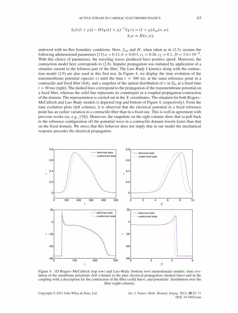
endowed with no-flux boundary conditions. Here, Iion and H , when taken as in (2.3), assume thefollowing adimensional parameters [13] aD 0.13, b D 0.013, c1 D 0.26, c2 D 0.1,D D 5.6�10�3.With this choice of parameters, the traveling waves produced have positive speed. Moreover, thecontraction model here corresponds to (2.8). Impulse propagation was initiated by application of astimulus current to the leftmost part of the fiber. The Luo–Rudy I kinetics along with the contrac-tion model (2.9) are also used in this first test. In Figure 4, we display the time evolution of thetransmembrane potential (species v) until the time t D 300 ms, at the same reference point in acontractile and fixed fiber (left), and a snapshot of the spatial distribution of v in �o at a fixed timet D 80ms (right). The dashed lines correspond to the propagation of the transmembrane potential ona fixed fiber, whereas the solid line represents its counterpart in a coupled propagation-contractionof the domain. The representation is carried out in theX -coordinates. The situation for both Rogers–McCulloch and Luo–Rudy models is depicted (top and bottom of Figure 4, respectively). From thetime evolution plots (left column), it is observed that the electrical potential in a fixed referencepoint has an earlier variation in a contractile fiber than in a fixed one. This is well in agreement withprevious works (as, e.g., [34]). Moreover, the snapshots on the right column show that (a pull backto the reference configuration of) the potential wave in a contractile domain travels faster than thaton the fixed domain. We stress that this behavior does not imply that in our model the mechanicalresponse precedes the electrical propagation.
0 100 200 300 400 500
0
0.2
0.4
0.6
0.8deformed stateundeformed state
0 2 4 6 8 10
0
0.2
0.4
0.6
0.8deformed stateundeformed state
0 100 200 300−90
−60
−30
0
30deformed stateundeformed state
0 2 4 6−90
−60
−30
0
30deformed stateundeformed state
Figure 4. 1D Rogers–McCulloch (top row) and Luo–Rudy (bottom row) monodomain models: time evo-lution of the membrane potentials (left column) in the pure electrical propagation (dashed lines) and in thecoupling with a description for the contraction of the fiber (solid lines), and potentials’ distribution over the
fiber (right column).
Copyright © 2011 John Wiley & Sons, Ltd. Int. J. Numer. Meth. Biomed. Engng. 2012; 28:52–71DOI: 10.1002/cnm
64 F. NOBILE, A. QUARTERONI AND R. RUIZ-BAIER
4.2. A 2D slab of tissue
In order to validate our mechanical numerical scheme (following [31]), we perform one time-stepiteration, so that all potential fields are known constant quantities acting as initial conditions. Thesystem to solve corresponds to (2.14) on the spatial domain �o D .�1, 1/2. A stretching in theX1-direction is assumed, along with a compression in the X2-direction. Let us define �D 1CˇX1.The given body force and boundary data (zero displacements on the bottom and traction on theremaining edges of the slab) are chosen such that the solution of the mechanical problem is
uD�ˇX21=2,X2.1C ˇX1/�1 �X2
�T, p D �1=2, which gives
FD
1C ˇX1 0
�X2.1C ˇX1/�2 .1C ˇX1/
�1
�,
and satisfies the incompressibility condition.Analogously, we perform a validation of the electrical solver, taking only the monodomain
Rogers–McCulloch problem (see, e.g., [5]). Non-homogeneous Dirichlet boundary conditions areimposed on the boundaries of the unit square, v.X1,X2, t / D k.t/, where k.�/ and the modelparameters are chosen such that the problem possesses the following analytical solution
v.X1,X2, t /Dn1C 0.001 exp
�p1=2.X1 � b0t /
�o�1.
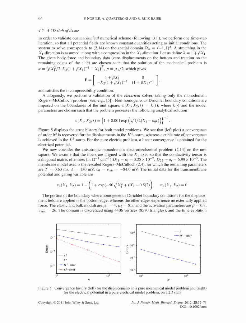
Figure 5 displays the error history for both model problems. We see that (left plot) a convergenceof order h2 is recovered for the displacements in theH 1-norm, whereas a cubic rate of convergenceis achieved in the L2-norm. For the pure electric problem, a linear convergence is obtained for theelectrical potential.
We now consider the anisotropic monodomain electromechanical problem (2.14) on the unitsquare. We assume that the fibers are aligned with the X1-axis, so that the conductivity tensor isa diagonal matrix of entries (in ��1 cm�1) D11 D �l D 3.28� 10�2, D22 D �t D 6.99� 10�3. Themembrane model used is the rescaled Rogers–McCulloch (2.4), for which the remaining parametersare T D 0.63 ms, A D 130 mV, v0 D vmin D �84.0 mV. The initial data for the transmembranepotential and gating variable are
v0.X1,X2/D 1�
�1C exp.�50
qX21 C .X2 � 0.5/2/
�, w0.X1,X2/D 0.
The portion of the boundary where homogeneous Dirichlet boundary conditions for the displace-ment field are applied is the bottom edge, whereas the other edges experience no externally appliedforce. The elastic and bulk moduli are �1 D 4, �2 D 8.5, and the activation parameters are ˇ D 0.3,vmax D 26. The domain is discretized using 4406 vertices (8570 triangles), and the time evolution
101 102
10−6
10−4
10−2
N
Err
ors
h2
h3
H 1−error
L 2−error
101 102
10−4
10−3
10−2
10−1
N
Err
ors
h
H 1− error
Figure 5. Convergence history (left) for the displacements in a pure mechanical model problem and (right)for the electrical potential in a pure electrical model problem, on a 2D slab.
Copyright © 2011 John Wiley & Sons, Ltd. Int. J. Numer. Meth. Biomed. Engng. 2012; 28:52–71DOI: 10.1002/cnm
ACTIVE STRAIN IN CARDIAC ELECTROMECHANICS 65
parameters are set to Tfinal D 600 ms, �t D 1 ms. A tolerance of 1.0� 10�5 is used for the Newtonstopping criterion (3.6), achieving convergence almost always in less than five iterations.
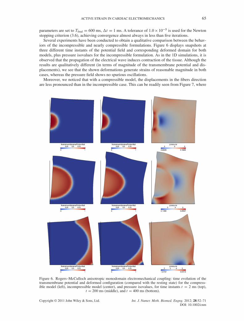
Several experiments have been conducted to obtain a qualitative comparison between the behav-iors of the incompressible and nearly compressible formulations. Figure 6 displays snapshots atthree different time instants of the potential field and corresponding deformed domain for bothmodels, plus pressure isovalues for the incompressible formulation. As in the 1D simulations, it isobserved that the propagation of the electrical wave induces contraction of the tissue. Although theresults are qualitatively different (in terms of magnitude of the transmembrane potential and dis-placements), we see that the shown deformations generate strains of reasonable magnitude in bothcases, whereas the pressure field shows no spurious oscillations.
Moreover, we noticed that with a compressible model, the displacements in the fibers directionare less pronounced than in the incompressible case. This can be readily seen from Figure 7, where
Figure 6. Rogers–McCulloch anisotropic monodomain electromechanical coupling: time evolution of thetransmembrane potential and deformed configuration (compared with the resting state) for the compress-ible model (left), incompressible model (center), and pressure isovalues, for time instants t D 2 ms (top),
t D 200 ms (middle), and t D 400 ms (bottom).
Copyright © 2011 John Wiley & Sons, Ltd. Int. J. Numer. Meth. Biomed. Engng. 2012; 28:52–71DOI: 10.1002/cnm
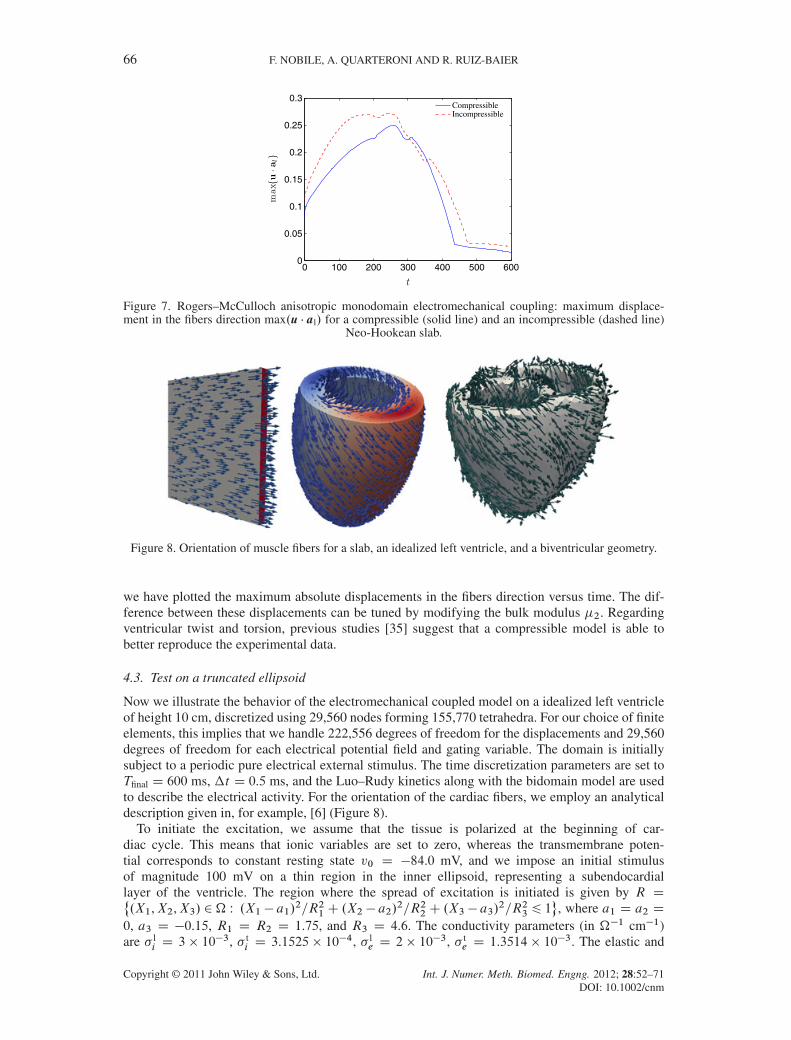
66 F. NOBILE, A. QUARTERONI AND R. RUIZ-BAIER
0 100 200 300 400 500 6000
0.05
0.1
0.15
0.2
0.25
0.3CompressibleIncompressible
Figure 7. Rogers–McCulloch anisotropic monodomain electromechanical coupling: maximum displace-ment in the fibers direction max.u � al/ for a compressible (solid line) and an incompressible (dashed line)
Neo-Hookean slab.
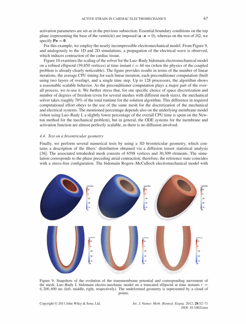
Figure 8. Orientation of muscle fibers for a slab, an idealized left ventricle, and a biventricular geometry.
we have plotted the maximum absolute displacements in the fibers direction versus time. The dif-ference between these displacements can be tuned by modifying the bulk modulus �2. Regardingventricular twist and torsion, previous studies [35] suggest that a compressible model is able tobetter reproduce the experimental data.
4.3. Test on a truncated ellipsoid
Now we illustrate the behavior of the electromechanical coupled model on a idealized left ventricleof height 10 cm, discretized using 29,560 nodes forming 155,770 tetrahedra. For our choice of finiteelements, this implies that we handle 222,556 degrees of freedom for the displacements and 29,560degrees of freedom for each electrical potential field and gating variable. The domain is initiallysubject to a periodic pure electrical external stimulus. The time discretization parameters are set toTfinal D 600 ms, �t D 0.5 ms, and the Luo–Rudy kinetics along with the bidomain model are usedto describe the electrical activity. For the orientation of the cardiac fibers, we employ an analyticaldescription given in, for example, [6] (Figure 8).
To initiate the excitation, we assume that the tissue is polarized at the beginning of car-diac cycle. This means that ionic variables are set to zero, whereas the transmembrane poten-tial corresponds to constant resting state v0 D �84.0 mV, and we impose an initial stimulusof magnitude 100 mV on a thin region in the inner ellipsoid, representing a subendocardiallayer of the ventricle. The region where the spread of excitation is initiated is given by R D˚.X1,X2,X3/ 2� W .X1 � a1/2=R21 C .X2 � a2/
2=R22 C .X3 � a3/2=R23 6 1
�, where a1 D a2 D
0, a3 D �0.15, R1 D R2 D 1.75, and R3 D 4.6. The conductivity parameters (in ��1 cm�1)are � l
i D 3 � 10�3, � ti D 3.1525 � 10�4, � l
e D 2 � 10�3, � te D 1.3514 � 10�3. The elastic and
Copyright © 2011 John Wiley & Sons, Ltd. Int. J. Numer. Meth. Biomed. Engng. 2012; 28:52–71DOI: 10.1002/cnm
ACTIVE STRAIN IN CARDIAC ELECTROMECHANICS 67
activation parameters are set as in the previous subsection. Essential boundary conditions on the topplane (representing the base of the ventricle) are imposed (u �nD 0), whereas on the rest of @�, wespecify PnD 0.
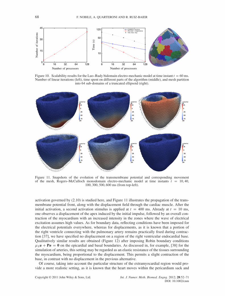
For this example, we employ the nearly incompressible electromechanical model. From Figure 9,and analogously to the 1D and 2D simulations, a propagation of the electrical wave is observed,which induces contraction of the cardiac tissue.
Figure 10 examines the scaling of the solver for the Luo–Rudy bidomain electromechanical modelon a refined ellipsoid (39,850 vertices) at time instant t D 60 ms (when the physics of the coupledproblem is already clearly noticeable). The figure provides results in terms of the number of lineariterations, the average CPU timing for each linear iteration, each preconditioner computation (builtusing two layers of overlap), and a single time step. Up to 128 processors, the algorithm showsa reasonable scalable behavior. As the preconditioner computation plays a major part of the over-all process, we re-use it. We further stress that, for our specific choice of space discretization andnumber of degrees of freedom (even for several meshes with different mesh sizes), the mechanicalsolver takes roughly 70% of the total runtime for the solution algorithm. This difference in requiredcomputational effort obeys to the use of the same mesh for the discretization of the mechanicaland electrical systems. The mentioned percentage depends also on the underlying membrane model(when using Luo–Rudy I, a slightly lower percentage of the overall CPU time is spent on the New-ton method for the mechanical problem), but in general, the ODE systems for the membrane andactivation function are almost perfectly scalable, as there is no diffusion involved.
4.4. Test on a biventricular geometry
Finally, we perform several numerical tests by using a 3D biventricular geometry, which con-tains a description of the fibers’ distribution obtained via a diffusion tensor statistical analysis[36]. The associated tetrahedral mesh consists of 6598 vertices and 30,309 elements. The simu-lation corresponds to the phase preceding atrial contraction; therefore, the reference state coincideswith a stress-free configuration. The bidomain Rogers–McCulloch electromechanical model with
Figure 9. Snapshots of the evolution of the transmembrane potential and corresponding movement ofthe mesh, Luo–Rudy I, bidomain electro-mechanic model on a truncated ellipsoid at time instants t D6, 200, 600 ms (left, middle, right, respectively). The undeformed geometry is represented by a cloud of
points.
Copyright © 2011 John Wiley & Sons, Ltd. Int. J. Numer. Meth. Biomed. Engng. 2012; 28:52–71DOI: 10.1002/cnm
68 F. NOBILE, A. QUARTERONI AND R. RUIZ-BAIER
8 16 32 64 1280
15
30
45
Number of processors
Num
ber
ofit
erat
ions
8 16 32 64 128
10
50
120
Number of processors
Tim
e(s
)
GMRES iterationPrecond. computationOne time step
Figure 10. Scalability results for the Luo–Rudy bidomain electro-mechanic model at time instant t D 60ms.Number of linear iterations (left), time spent on different parts of the algorithm (middle), and mesh partition
into 64 sub-domains of a truncated ellipsoid (right).
Figure 11. Snapshots of the evolution of the transmembrane potential and corresponding movementof the mesh, Rogers–McCulloch monodomain electro-mechanic model at time instants t D 10, 40,
100, 300, 500, 600 ms (from top-left).
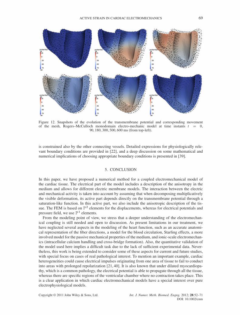
activation governed by (2.10) is studied here, and Figure 11 illustrates the propagation of the trans-membrane potential front, along with the displacement field through the cardiac muscle. After theinitial activation, a second activation stimulus is applied at t D 400 ms. Already at t D 10 ms,one observes a displacement of the apex induced by the initial impulse, followed by an overall con-traction of the myocardium with an increased intensity in the zones where the wave of electricalexcitation assumes high values. As for boundary data, reflecting conditions have been imposed forthe electrical potentials everywhere, whereas for displacements, as it is known that a portion ofthe right ventricle connecting with the pulmonary artery remains practically fixed during contrac-tion [37], we have specified no displacement on a region of the right ventricular endocardial base.Qualitatively similar results are obtained (Figure 12) after imposing Robin boundary conditions�1uC Pn D 0 on the epicardial and basal boundaries. As discussed in, for example, [38] for thesimulation of arteries, this setting may be regarded as an elastic resistance of the tissues surroundingthe myocardium, being proportional to the displacement. This permits a slight contraction of thebase, in contrast with no displacement in the previous alternative.
Of course, taking into account the particular structure of the extramyocardial region would pro-vide a more realistic setting, as it is known that the heart moves within the pericardium sack and
Copyright © 2011 John Wiley & Sons, Ltd. Int. J. Numer. Meth. Biomed. Engng. 2012; 28:52–71DOI: 10.1002/cnm
ACTIVE STRAIN IN CARDIAC ELECTROMECHANICS 69
Figure 12. Snapshots of the evolution of the transmembrane potential and corresponding movementof the mesh, Rogers–McCulloch monodomain electro-mechanic model at time instants t D 0,
90, 180, 300, 500, 600 ms (from top-left).
is constrained also by the other connecting vessels. Detailed expressions for physiologically rele-vant boundary conditions are provided in [22], and a deep discussion on some mathematical andnumerical implications of choosing appropriate boundary conditions is presented in [39].
5. CONCLUSION
In this paper, we have proposed a numerical method for a coupled electromechanical model ofthe cardiac tissue. The electrical part of the model includes a description of the anisotropy in themedium and allows for different electric membrane models. The interaction between the electricand mechanical activity is taken into account by assuming that when decomposing multiplicativelythe visible deformation, its active part depends directly on the transmembrane potential through asaturation-like function. In this active part, we also include the anisotropic description of the tis-sue. The FEM is based on P2 elements for the displacements, whereas for electrical potentials andpressure field, we use P1 elements.
From the modeling point of view, we stress that a deeper understanding of the electromechan-ical coupling is still needed and open to discussion. As present limitations in our treatment, wehave neglected several aspects in the modeling of the heart function, such as an accurate anatomi-cal representation of the fiber directions, a model for the blood circulation, Starling effects, a moreinvolved model for the passive mechanical properties of the medium, and ionic-scale electromechan-ics (intracellular calcium handling and cross-bridge formation). Also, the quantitative validation ofthe model used here implies a difficult task due to the lack of sufficient experimental data. Never-theless, this work is being extended to consider some of these aspects for current and future studies,with special focus on cases of real pathological interest. To mention an important example, cardiacheterogeneities could cause electrical impulses originating from one area of tissue to fail to conductinto areas with prolonged repolarization [21, 40]. It is also known that under dilated myocardiopa-thy, which is a common pathology, the electrical potential is able to propagate through all the tissue,whereas there are specific regions of the ventricular chamber where no contraction takes place. Thisis a clear application in which cardiac electromechanical models have a special interest over pureelectrophysiological models.
Copyright © 2011 John Wiley & Sons, Ltd. Int. J. Numer. Meth. Biomed. Engng. 2012; 28:52–71DOI: 10.1002/cnm
70 F. NOBILE, A. QUARTERONI AND R. RUIZ-BAIER
From the numerical viewpoint, several improvements can be rather straightforwardly includedin the proposed method. First of all, the time-stepping strategy could be upgraded to an adaptivescheme by using a similar algorithm as the one proposed in [6], where the use of a small time step inthe excitation phase would increase the accuracy in capturing the action potential upstroke, whereasa large time step could be used for the plateau phase. Secondly, other finite element discretiza-tions and more sophisticated preconditioning algorithms are sought, such as the monodomain-basedblock-triangular preconditioning proposed in [7] or structured algebraic multigrid preconditionersin the spirit of [8].
Finally, to the authors’ knowledge, the well-posedness analysis, global existence, regularity ofsolutions, and related questions concerning the mathematical study of cardiac electromechanicalmodels have not been thoroughly addressed. Although a rigorous analysis in this direction is cur-rently under development [28], we can anticipate that the main difficulty lies in treating the geomet-rical nonlinearity introduced in the electrical diffusion operator by the change of coordinates fromEulerian to Lagrangian. A possible way to circumvent this issue consists in considering a linearizedcontribution of the mechanical response on the bidomain equations, or alternatively, applying atruncation operator that eventually allows us to bound the coupling term .ICru/�1Dk.ICru/�T .
ACKNOWLEDGEMENTS
The authors gratefully acknowledge the discussions with Davide Ambrosi regarding the active strain for-mulation. This work has been supported by the European Research Council through the advanced grant“Mathcard, Mathematical Modelling and Simulation of the Cardiovascular System”, project ERC-2008-AdG227058.
REFERENCES
1. Cherubini C, Filippi S, Nardinocchi P, Teresi L. An electromechanical model of cardiac tissue: constitutive issuesand electrophysiological effects. Progresses in Biophysics and Molecular Biology 2008; 97:562–573.
2. Nash MP, Panfilov AV. Electromechanical model of excitable tissue to study reentrant cardiac arrhythmias.Progresses in Biophysics and Molecular Biology 2004; 85:501–522.
3. Pathmanathan P, Whiteley JP. A numerical method for cardiac mechanoelectric simulations. Annals of BiomedicalEngineering 2009; 37:860–873.
4. Sainte-Marie J, Chapelle D, Cimrman R, Sorine M. Modeling and estimation of the cardiac electromechanicalactivity. Computers and Structures 2006; 84:1743–1759.
5. Bendahmane M, Bürger R, Ruiz-Baier R. A multiresolution space–time adaptive scheme for the bidomain model inelectrocardiology. Numerical Methods for Partial Differential Equations 2010; 26:1377–1404.
6. Colli Franzone P, Pavarino LF. A parallel solver for reaction–diffusion systems in computational electro-cardiology.Mathematical Models and Methods in Applied Sciences 2004; 14:883–911.
7. Gerardo-Giorda L, Mirabella L, Nobile F, Perego M, Veneziani A. A model-based block-triangular preconditionerfor the bidomain system in electrocardiology. Journal of Computational Physics 2009; 228:3625–3639.
8. Pennacchio M, Simoncini V. Algebraic multigrid preconditioners for the bidomain reaction–diffusion system.Applied Numerical Mathematics 2009; 59:3033–3050.
9. Ambrosi D, Arioli G, Nobile F, Quarteroni A. Electromechanical coupling in cardiac dynamics: the active strainapproach. SIAM Journal of Applied Mathematics 2011; 71:605–621.
10. Nardinocchi P, Teresi L. On the active response of soft living tissues. Journal of Elasticity 2007; 88:27–39.11. Ravens U. Mechano-electric feedback and arrhythmias. Progresses in Biophysics and Molecular Biology 2003;
82:255–266.12. Tung L. A bi-domain model for describing ischemic myocardial D-C currents. PhD thesis, MIT, Cambridge, MA,
1978.13. Rogers JM, McCulloch AD. A collocation-Galerkin finite element model of cardiac action potential propagation.
IEEE Transactions on Biomedical Engineering 1994; 41:743–757.14. Luo C, Rudy Y. A model of the ventricular cardiac action potential: depolarization, repolarization, and their
interaction. Circulation Research 1991; 68:1501–1526.15. Bürger R, Ruiz-Baier R. Adaptive multiresolution simulation of waves in electrocardiology. In Numerical Mathe-
matics and Advanced Applications. Kreiss G, et al (eds). Springer-Verlag: Berlin Heidelberg, 2010; 199–207.16. Holzapfel GA, Ogden RW. Constitutive modelling of passive myocardium: a structurally based framework for
material characterization. Philosophical Transactions of the Royal Society A 2009; 367:3445–3475.17. Simo JC, Pister KS. Remarks on rate constitutive equations for finite deformations. Computational Methods in
Applied Mechanics and Engineering 1984; 46:201–215.18. Taber LA, Perucchio R. Modeling heart development. Journal of Elasticity 2000; 61:165–197.
Copyright © 2011 John Wiley & Sons, Ltd. Int. J. Numer. Meth. Biomed. Engng. 2012; 28:52–71DOI: 10.1002/cnm
ACTIVE STRAIN IN CARDIAC ELECTROMECHANICS 71
19. Nash MP, Hunter PJ. Computational mechanics of the heart. Journal of Elasticity 2000; 61:113–141.20. Ciarlet PG. Mathematical Elasticity, Vol. 1. Three Dimensional Elasticity. North-Holland: Amsterdam, 1998.21. Kerckhoffs R, Bovendeerd P, Kotte JC, Prinzen F, Smiths K, Arts T. Homogeneity of cardiac contraction despite
physiological asynchrony of depolarization: a model study. Annals of Biomedical Engineering 2003; 31:536–547.22. Usyk TP, LeGrice IJ, McCulloch AD. Computational model of three-dimensional cardiac electromechanics.
Computing and Visualization in Science 2002; 4:249–257.23. Rossi S, Ruiz-Baier R, Pavarino LF, Quarteroni A. Active strain and activation models in cardiac mechanics.
Submitted.24. Rice JJ, Wang F, Bers DM, de Tombe PP. Approximate model of cooperative activation and crossbridge cycling in
cardiac muscle using ordinary differential equations. Biophysical Journal 2008; 95:2368–2390.25. Colli Franzone P, Savaré G. Degenerate evolution systems modeling the cardiac electric field at micro- and macro-
scopic level. In Evolution Equations, Semigroups and Functional Analysis, Lorenzi A, Ruf B (eds). Birkhäuser:Basel, 2002; 49–78.
26. Veneroni M. Reaction–diffusion systems for the macroscopic Bidomain model of the cardiac electric field. NonlinearAnalysis: Real World Applications 2009; 10:849–868.
27. Krejcí P, Sainte-Marie J, Sorine M, Urquiza JM. Solutions to muscle fiber equations and their long time behaviour.Nonlinear Analysis: Real World Applications 2006; 7:535–558.
28. Andreianov B, Bendahmane M, Quarteroni A, Ruiz-Baier R. Mathematical analysis of a coupled model in cardiacelectromechanics. Submitted.
29. Göktepe S, Kuhl E. Electromechanics of the heart: a unified approach to the strongly coupled excitation–contractionproblem. Computational Mechanics 2010; 45:227–243.
30. Quarteroni A. Numerical models for differential problems, MS&A series, Vol. 2. Springer-Verlag: Milan, 2009.31. Pathmanathan P, Gavaghan D, Whiteley JP. A comparison of numerical methods used for finite element modelling
of soft tissue deformation. Journal of Strain Analysis 2009; 44:391–406.32. LifeV library. http://www.lifev.org.33. Hecht F. FREEFEM++, 3rd edn. Université Pierre et Marie Curie, Laboratoire Jacques-Louis Lions: Paris, 2008.34. Vetter FJ, Rogers JM, McCulloch AD. A finite element model of passive mechanics and electrical propagation in the
rabbit ventricles. Computational Cardiology 1998; 25:705–708.35. Taber LA, Yang M, Podzus WW. Mechanics of ventricular torsion. Journal of Biomechanics 1996; 29:745–752.36. Peyrat JM, Sermesant M, Pennec X, Delingette H, Xu C, McVeigh ER, Ayache N. A computational framework for the
statistical analysis of cardiac diffusion tensors: application to a small database of canine hearts. IEEE Transactionson Medical Imaging 2007; 26:1500–1514.
37. Gurev V, Lee T, Constantino J, Arevalo H, Trayanova NA. Models of cardiac electromechanics based on individualhearts imaging data. Biomechanics and modeling in mechanobiology 2011; 10:295–306.
38. Moireau P, Xiao N, Astorino M, Figueroa CA, Chapelle D, Taylor CA, Gerbeau JF. External tissue support andfluid-structure simulation in blood flows. Biomechanics and Modeling in Mechanobiology 2011, to appear.
39. Pathmanathan P, Chapman SJ, Gavaghan D, Whiteley JP. Cardiac electromechanics: the effect of contraction modelon the mathematical problem and accuracy of the numerical scheme. Quarterly Journal of Mechanics and AppliedMathematics 2010; 63:375–399.
40. Trayanova NA. Whole-heart modeling: applications to cardiac electrophysiology and electromechanics. CirculationResearch 2011; 108:113–128.
Copyright © 2011 John Wiley & Sons, Ltd. Int. J. Numer. Meth. Biomed. Engng. 2012; 28:52–71DOI: 10.1002/cnm


![Electromechanical wave imaging and electromechanical wave … · 2019-07-23 · motion and strain estimation based on Bmode [9] or radio-frequency (RF) ultrasound signals [10–13]](https://img.pdfslide.net/doc/110x75/5e9f95fa3886094c5e322e3d/electromechanical-wave-imaging-and-electromechanical-wave-2019-07-23-motion-and.jpg)