Embed Size (px)
Citation preview
An Adaptive Control Algorithm for Maximum
Power Point Tracking for Wind Energy
Conversion Systems
by
Joanne Hui
A thesis submitted to the
Department of Electrical and Computer Engineering
in conformity with the requirements for
the degree of Master of Science (Engineering)
Queen’s University
Kingston, Ontario, Canada
December 2008
Copyright c© Joanne Hui, 2008

Abstract
Wind energy systems are being closely studied because of its benefits as an envi-
ronmentally friendly and renewable source of energy. Because of its unpredictable
availability, power management concepts are essential to extract as much power as
possible from the wind when it becomes available.
The purpose of this thesis is to presents a new adaptive control algorithm for
maximum power point tracking (MPPT) in wind energy systems. The proposed con-
trol algorithm allows the generator to track the optimal operation points of the wind
turbine system under fluctuating wind conditions and the tracking process speeds
up over time. This algorithm does not require the knowledge of intangible turbine
mechanical characteristics such as its power coefficient curve, power characteristic or
torque characteristic. The algorithm uses its memory feature to adapt to any given
wind turbine and to infer the optimum rotor speeds for wind speeds that have not
occurred before. The proposed algorithm uses a modified version of Hill Climb Search
(HCS) and intelligent memory to implement its power management scheme. This al-
gorithm is most suitable for smaller grid or battery connected wind energy systems.
PSIM simulation studies have been done to confirm the effectiveness of the proposed
algorithm.
i

Acknowledgments
First and foremost I would like to thank my supervisor Dr. Alireza Bakhshai for
his wisdom and guidance. Secondly I would like to thank my mom, Rosalind Li, for
giving me unconditional love and support throughout my academic career. I would
also like to thank all the professors that have taught me throughout my years at
Queen’s. Lastly, for their advice, support and laughter, I would like to acknowledge
all of my fellow ePEARL colleagues; special thanks to John, Ali and Majid.
ii

Glossary
Cp Power Coefficient
β Pitch Angle
tm Turbine Mechanical Torque
pm Turbine Mechanical Power
ω Angular Speed
Cp Power Coefficient
Cp,max Power coefficient value that results in maximum
power transfer
Pout Output Power
Vdc DC Link Voltage
If Generator Field Current
Ig Load Current
Idm Demanded Current
Pdm Power Demanded
ωref Reference Angular Speed
ωgen Generator Angular Speed
λopt Optimal Tip-Speed Ratio
iii

Glossary iv
vw Wind Velocity
ωopt Optimal Angular Speed
G Gear Ratio
R Turbine Blade Radius
Lmax Maximum Boost Converter Inductor Value
Cmin Mininmum Output Capacitor Value
d Duty Ratio
MPPT Maximum Power Point Tracking
HCS Hill Climb Searching
WECS Wind Energy Conversion System
TSR (λ) Tip-Speed Ratio
CDL Change Detection Loop
OPAL Operating Point Adjustment Loop
WECS Wind Energy Conversion System
WFSG Wound Field Synchronous Generator
SCIG Squirrel Cage Induction Generator
PWM Pulse Width Modulation
PMSG Permanent Magnet Synchronous Generator
DFIG Doubly Fed Wound Rotor Induction Generator
AHCS Advanced Hill Climb Search
MPED Max-Power Error Driven
DCM Discontinuous Conduction Model

Glossary v
FPGA Field Programmable Gate Array
DSP Digital Signal Processor

Table of Contents
Abstract i
Acknowledgments ii
Glossary iii
Table of Contents vi
List of Tables ix
List of Figures x
Chapter 1:
Introduction . . . . . . . . . . . . . . . . . . . . . . . . . . 1
1.1 Wind Energy Market . . . . . . . . . . . . . . . . . . . . . . . . . . . 2
1.2 Wind Energy Conversion Principles . . . . . . . . . . . . . . . . . . . 4
1.3 Concept of Maximum Power Extraction . . . . . . . . . . . . . . . . . 9
1.4 Concept of Proposed Algorithm . . . . . . . . . . . . . . . . . . . . . 11
1.5 Organization of Thesis . . . . . . . . . . . . . . . . . . . . . . . . . . 12
Chapter 2:
Wind Energy Conversion Systems . . . . . . . . . . . . . 14
vi

TABLE OF CONTENTS vii
2.1 Wind Turbine Technology . . . . . . . . . . . . . . . . . . . . . . . . 14
2.2 Types of Horizontal-Axis Wind Turbines . . . . . . . . . . . . . . . . 16
2.3 Types of Wind Energy Conversion Systems (WECS) . . . . . . . . . 17
2.4 Configurations of Variable Speed Wind Conversion Systems . . . . . 20
2.5 Literature Review of Maximum Power Extraction Techniques . . . . . 26
Chapter 3:
Proposed Algorithm . . . . . . . . . . . . . . . . . . . . . 34
3.1 Algorithm Concept and Features . . . . . . . . . . . . . . . . . . . . 34
3.2 Algorithm Implementation . . . . . . . . . . . . . . . . . . . . . . . . 41
Chapter 4:
System Modelling . . . . . . . . . . . . . . . . . . . . . . . 50
4.1 Wind Turbine Modelling . . . . . . . . . . . . . . . . . . . . . . . . . 51
4.2 Power Electronic Interface Analysis . . . . . . . . . . . . . . . . . . . 57
Chapter 5:
Algorithm Performance . . . . . . . . . . . . . . . . . . . 65
5.1 Simulation Model Overview . . . . . . . . . . . . . . . . . . . . . . . 65
5.2 Algorithm Operation . . . . . . . . . . . . . . . . . . . . . . . . . . . 66
5.3 Results Summary . . . . . . . . . . . . . . . . . . . . . . . . . . . . . 73
Chapter 6:
Summary and Conclusions . . . . . . . . . . . . . . . . . 74
6.1 Summary . . . . . . . . . . . . . . . . . . . . . . . . . . . . . . . . . 74
6.2 Contributions . . . . . . . . . . . . . . . . . . . . . . . . . . . . . . . 76

TABLE OF CONTENTS viii
6.3 Future Works . . . . . . . . . . . . . . . . . . . . . . . . . . . . . . . 77
6.4 Conclusion . . . . . . . . . . . . . . . . . . . . . . . . . . . . . . . . . 78
Bibliography . . . . . . . . . . . . . . . . . . . . . . . . . . . . . . . . . 79

List of Tables
4.1 Customized wind turbine parameters . . . . . . . . . . . . . . . . . . 53
4.2 Design specifications for boost converter. . . . . . . . . . . . . . . . . 58
5.1 The algorithm’s decisions represented by values. *NOTE: flag = 3
cannot be observed in the output graphs, as it is an internal flag to
invoke certain actions. . . . . . . . . . . . . . . . . . . . . . . . . . . 68
ix

List of Figures
1.1 the total amount of globally installed wind energy systems per year [1]. 3
1.2 the total amount of the newly installed wind energy systems around
the world per year [1]. . . . . . . . . . . . . . . . . . . . . . . . . . . 4
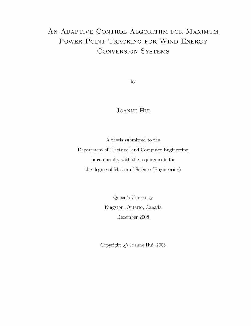
1.3 a:Total installed WECS distribution (as of 2006); b:Newly installed
WECS distribution(as of 2006) [2]. . . . . . . . . . . . . . . . . . . . 5
1.4 a:Total installed WECS distribution (as of 2007); b:Newly installed
WECS distribution(as of 2007) [1]. . . . . . . . . . . . . . . . . . . . 6
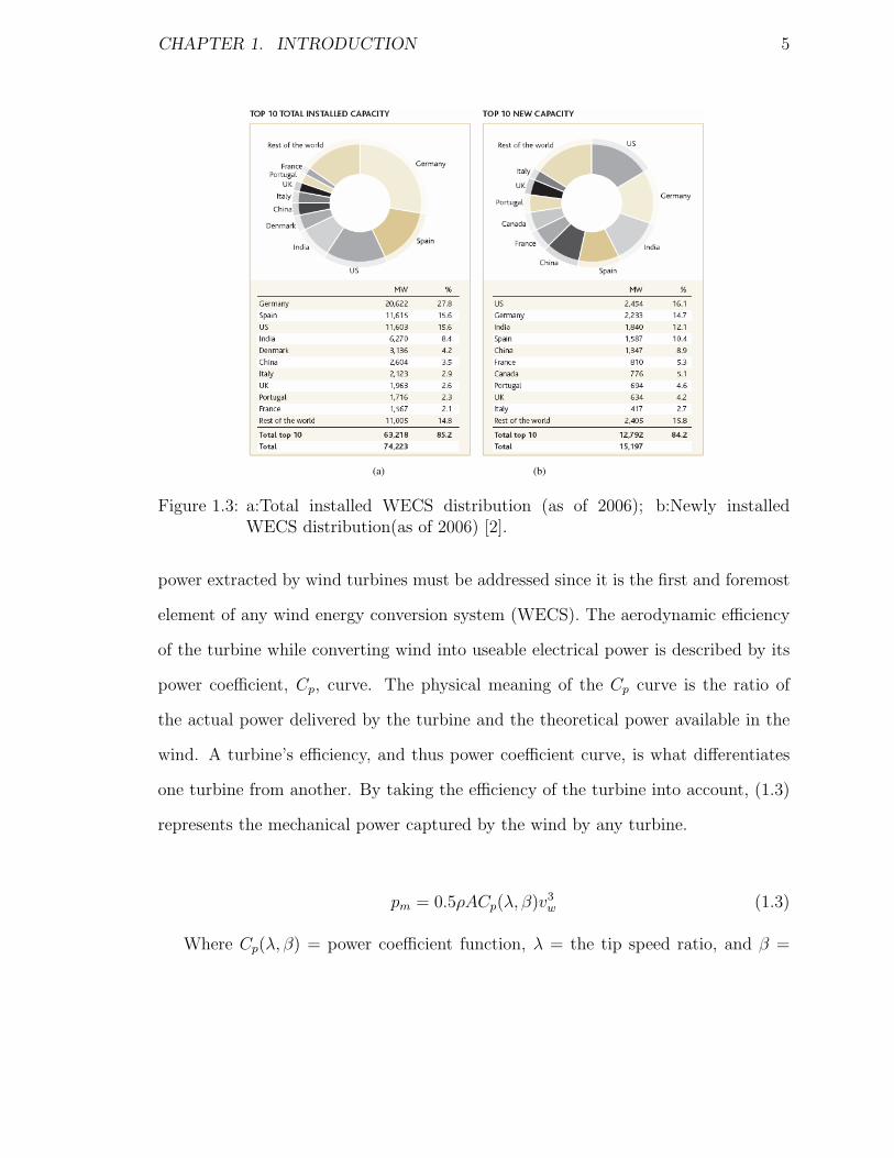
1.5 A typical power coefficient curve of a fixed-pitch wind turbine. . . . . 8
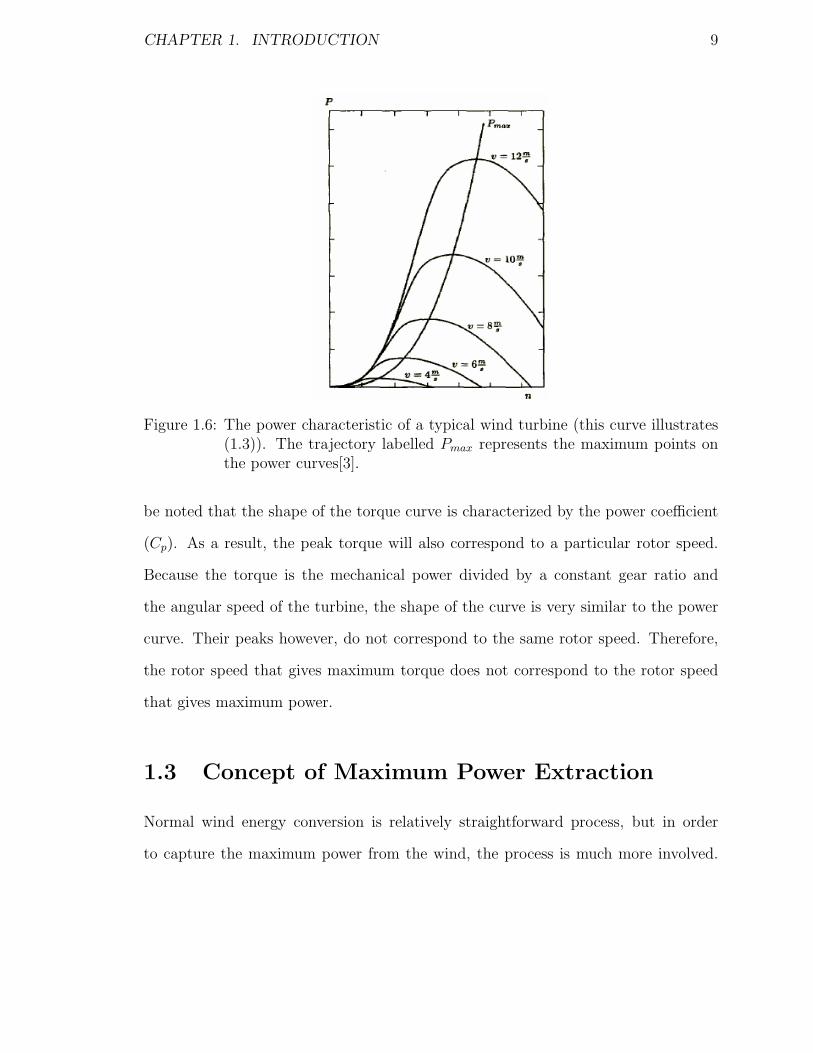
1.6 The power characteristic of a typical wind turbine (this curve illustrates
(1.3)). The trajectory labelled Pmax represents the maximum points
on the power curves[3]. . . . . . . . . . . . . . . . . . . . . . . . . . . 9
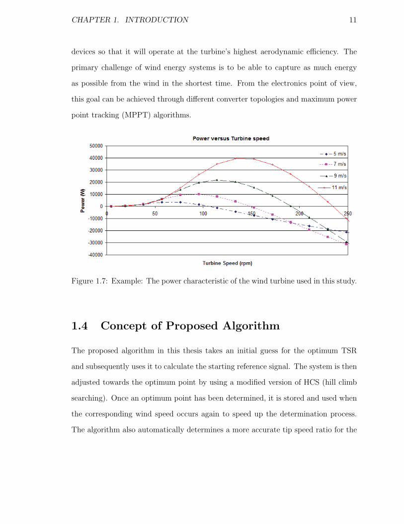
1.7 Example: The power characteristic of the wind turbine used in this
study. . . . . . . . . . . . . . . . . . . . . . . . . . . . . . . . . . . . 11
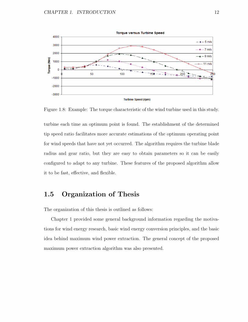
1.8 Example: The torque characteristic of the wind turbine used in this
study. . . . . . . . . . . . . . . . . . . . . . . . . . . . . . . . . . . . 12
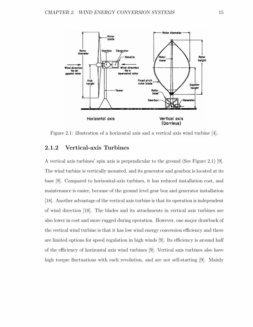
2.1 illustration of a horizontal axis and a vertical axis wind turbine [4]. . 15
2.2 A typical fixed speed wind turbine configuration [5]. . . . . . . . . . . 18
2.3 A typical fixed speed wind turbine configuration [5]. . . . . . . . . . . 21
x

LIST OF FIGURES xi
2.4 Common system setup with a permanent magnet wind turbine (genera-
tor is connected to the utility through a diode rectifier, boost converter
and an inverter) [6] . . . . . . . . . . . . . . . . . . . . . . . . . . . . 22
2.5 Common system setup with a permanent magnet wind turbine (gener-
ator is connected to the utility through two back-to-back converters)
[6]. . . . . . . . . . . . . . . . . . . . . . . . . . . . . . . . . . . . . . 23
2.6 Common system setup with a doubly fed wound rotor induction wind
turbine (the generator rotor is connected to the utility through two
back-to-back converters, and the stator is connected directly to the
utility)[6]. . . . . . . . . . . . . . . . . . . . . . . . . . . . . . . . . . 24
2.7 Common system setup with a squirrel cage induction generator (gen-
erator is connected to the utility through two back-to-back converters)
[6]. . . . . . . . . . . . . . . . . . . . . . . . . . . . . . . . . . . . . . 25
2.8 Affects of air density on the power extracted from the wind at 9 m/s. 29
2.9 a)Intelligent Memory Lookup Table ; b)Power characteristic of turbine
with respect to Vdc[7]. . . . . . . . . . . . . . . . . . . . . . . . . . . . 30
2.10 Maximum Power curves for different air densities. . . . . . . . . . . . 31
3.1 Wind power curve for an arbitrary wind speed. This figure illustrates
the concept of the “observe and perturb” of HCS. . . . . . . . . . . . 37
3.2 Illustration of proposed algorithm logic at the initial stage. . . . . . . 39
3.3 Illustration of proposed algorithm logic in the second stage (after initial
startup and when there is no change in wind speed). . . . . . . . . . 40
3.4 illustration of algorithm in the even of a wind speed change. . . . . . 41
3.5 Logic Flow of the proposed algorithm. . . . . . . . . . . . . . . . . . 42

LIST OF FIGURES xii
3.6 Illustration of the proposed algorithm’s adjustment process (startup). 46
3.7 Illustration of the proposed algorithm’s adjustment process (wind change
after startup). . . . . . . . . . . . . . . . . . . . . . . . . . . . . . . . 49
4.1 Wind energy conversion system block diagram. . . . . . . . . . . . . . 51
4.2 Cp Characteristic of Custom Wind Turbine Model. . . . . . . . . . . 52
4.3 Output Mechanical Power of Turbine versus the Turbine Speed (Air
density: 1.1 kpa). . . . . . . . . . . . . . . . . . . . . . . . . . . . . . 53
4.4 Output Mechanical Torque of Turbine versus the Turbine Speed (Air
density:1.1 kpa) . . . . . . . . . . . . . . . . . . . . . . . . . . . . . . 54
4.5 Custom Wind Turbine Structure (Air density: 1.1 kpa). . . . . . . . . 54
4.6 Custom Wind Turbine (Air density: 1.1 kpa). . . . . . . . . . . . . . 55
4.7 Example: An induction machine with a custom mechanical load model
in PSIM [8]. . . . . . . . . . . . . . . . . . . . . . . . . . . . . . . . . 56
4.8 The PSIM model of the fixed-pitch turbine. . . . . . . . . . . . . . . 56
4.9 Closed loop system. . . . . . . . . . . . . . . . . . . . . . . . . . . . . 60
4.10 Average circuit model of DCM boost converter. . . . . . . . . . . . . 61
4.11 Small signal equivalent circuit of DCM boost converter. . . . . . . . . 61
4.12 Relationship between Vo and generator speed (rpm). . . . . . . . . . . 63
4.13 Bode plot of overall closed loop system. . . . . . . . . . . . . . . . . . 64
5.1 Complete wind energy conversion system. . . . . . . . . . . . . . . . . 66
5.2 The Power Coefficient Curve of the Turbine (Optimum tip speed ratio
= 8.1 as indicated). . . . . . . . . . . . . . . . . . . . . . . . . . . . . 66
5.3 Turbine power curves for vw = 7m/s and for vw = 9m/s. ωopt,7 = 2707
rpm, and ωopt,9 = 3480 rpm. . . . . . . . . . . . . . . . . . . . . . . 67

LIST OF FIGURES xiii
5.4 Algorithm performance under a constant wind speed of 7 m/s. . . . . 69
5.5 Algorithm performance under a constant wind speed of 9 m/s. . . . . 70
5.6 Algorithm performance under a step change in wind speed (7 m/s to
9 m/s at time = 55s). . . . . . . . . . . . . . . . . . . . . . . . . . . . 71
5.7 Algorithm performance under two wind speed changes (7 m/s to 9 m/s
at time = 55s, 9 m/s to 7 m/s at time = 80s). . . . . . . . . . . . . 71
5.8 Illustration of the algorithm’s TSR determination process under two
wind speed changes (7 m/s to 9 m/s at time = 55s, 9 m/s to 7 m/s at
time = 80s). . . . . . . . . . . . . . . . . . . . . . . . . . . . . . . . 72
5.9 Illustration of the algorithm’s optimum point determination process
(speed adjustment and output power) under two wind speed changes
(7 m/s to 9 m/s at time = 55s, 9 m/s to 7 m/s at time = 80s). . . . 73

Chapter 1
Introduction
Due to the increasing concern about the environment and the depletion of natural
resources such as fossil fuels, much research is now focused on obtaining new environ-
mentally friendly sources of power. To preserve our planet for the future generations,
natural renewable sources are being closely studied and harvested for our energy
needs. Wind energy is environmentally friendly, inexhaustible, safe, and capable of
supplying substantial amounts of power. However, due to wind’s erratic nature, in-
telligent control strategies must be implemented to harvest as much potential wind
energy as possible while it is available. Because of its advantages, erratic nature, and
recent technological advancements in wind turbine aerodynamics and power electronic
interfaces, wind energy is considered to be an excellent supplementary energy source.
Research to extract the maximum power out of wind energy is an essential part of
making wind energy much more viable and attractive.
1

CHAPTER 1. INTRODUCTION 2
1.1 Wind Energy Market
Wind energy has been harnessed by many generations for thousands of years to mill
grain, pump water and sailing [9]. It wasn’t until the late nineteen century when
the development of a 12 kW windmill generator was used to generate electricity [9].
However, it was only in the 1980s that the technology has become mature enough
to efficiently and reliably produce electricity. Since then, many wind energy systems
have been developed and the technological advances have been phenomenal. Just in
last decade, the wind energy industry has experienced a growth of almost 30 percent
each year [2]. The global value of new wind energy plants installed in 2006 alone
has reached US $24 billion, and over 70 countries have wind turbine installations [2].
From 1996 to 2007, the total cumulative capacity of global wind power has increased
from 6.8 GW to 93.8 GW (See Figure 1.1) [1]. In particular, the last two years (2006
and 2007) have been record breaking years for the wind industry. Before 2007, 2006
had the highest ever amount of installations of wind energy systems in a single year,
reaching 15 GW (See Figure 1.2) [2]. Afterwards, the year 2007 became another
historical year as the total cumulative capacity of global wind power increased by
19.8 GW (27% growth) to reach a final total of 93.8 GW of installed wind power (See
Figure 1.2) [1].
Figure 1.3a and 1.3b show the distribution of the top ten countries with the highest
percentage of installed wind energy conversion systems (WECS) and the top ten
countries with the highest percentage of newly installed WECSs in 2006 respectively.
Not only is wind energy environmentally friendly, its development also strengthens
local economies and insulates the countries from macro-economical shocks of the
global commodities market (volatile gas, oil and coal prices) [2]. With continuous

CHAPTER 1. INTRODUCTION 3
Figure 1.1: the total amount of globally installed wind energy systems per year [1].
cost reductions in wind turbines, government incentive programs promoting wind
energy, and public demand for cleaner power sources, wind energy has become one
of the most promising and fastest growing energy resources in the world. As of 2006,
North America (mainly US and Canada), accounts for approximately 17.6% of the
global wind power installations [9]. With an 113% increase in new installations from
2005, 2006 was the most significant year for the wind industry in Canada. In 2006,
Canada was ranked 12th in the world with a total of 1.46 GW of installed wind
power, and ranked 7th for having a 0.78 GW of new installations [2]. As the interest
in wind energy continues, Canada has experienced its second best year in 2007 with
a 26% increase (386 MW) in new wind energy capacity [1]. As of 2007, Canada now
has 1846 MW of installed wind energy capacity and it is now ranked 10th in terms
of new installations (See Figure 1.4). As of 2008, Canada has signed contracts for
the installation of an additional 2.8 GW of wind energy by 2010. The Canadian
government hopes to have at least 10 GW of installed wind power by 2015. This
translates to a reduction of 12 million tons of greenhouse gas emissions [9]. Also

CHAPTER 1. INTRODUCTION 4
Figure 1.2: the total amount of the newly installed wind energy systems around theworld per year [1].
because of the geographical nature of the nation, Canada has more than enough wind
resources to meet 20% of its population’s electricity demand [10].
1.2 Wind Energy Conversion Principles
The classical equations of kinetic energy and power describe the potential energy that
can be harnessed from the wind. The kinetic energy available from wind is described
by (1.1) [11]. By classical physics theory, to translate kinetic energy into the power,
energy is divided by time; thus the power from the kinetic energy is given by (1.2).
Ek = 0.5mv2w = 0.5ρAdv2
w (1.1)
pw =0.5mvw
t=
0.5ρAdv2w
t= 0.5ρAv3
w (1.2)
Where ρ = air density, A = rotor swept area, d = distance, m = mass of air =
air density * volume = ρ*A*d, and Vw = distance/time.
With the theoretical power available in wind established by (1.1) and (1.2), the
CHAPTER 1. INTRODUCTION 5
(a) (b)
Figure 1.3: a:Total installed WECS distribution (as of 2006); b:Newly installedWECS distribution(as of 2006) [2].
power extracted by wind turbines must be addressed since it is the first and foremost
element of any wind energy conversion system (WECS). The aerodynamic efficiency
of the turbine while converting wind into useable electrical power is described by its
power coefficient, Cp, curve. The physical meaning of the Cp curve is the ratio of
the actual power delivered by the turbine and the theoretical power available in the
wind. A turbine’s efficiency, and thus power coefficient curve, is what differentiates
one turbine from another. By taking the efficiency of the turbine into account, (1.3)
represents the mechanical power captured by the wind by any turbine.
pm = 0.5ρACp(λ, β)v3w (1.3)
Where Cp(λ, β) = power coefficient function, λ = the tip speed ratio, and β =

CHAPTER 1. INTRODUCTION 6
Figure 1.4: a:Total installed WECS distribution (as of 2007); b:Newly installedWECS distribution(as of 2007) [1].
pitch angle.
From (1.3), it can be observed that the power available in the wind is proportional
to the cube of the wind speed. This means that there is much more energy in high-
speed winds than in slow winds. Also, since the power is proportional to the rotor
swept area, and thus to the square of the diameter, doubling the rotor diameter will
quadruple the available power. Air density also plays a role in the amount of available
mechanical power of the turbine; lower air densities (e.g. warm air) results in less
available power in wind. The power coefficient function, Cp(λ, β), is dependent on
two factors: i) the tip speed ratio (λ), and ii) the pitch angle (β). This function is
normally provided (in the form of a curve) by the wind turbine manufacturer since it
characterizes the efficiency of its wind turbines. If this curve is not provided, then it

CHAPTER 1. INTRODUCTION 7
can be obtained by performing field tests. The power coefficient can be evaluated by
(1.4).
Cp(λ, β) =actualturbinepower
theoreticalwindpower=
pm
pw
=pm
0.5ρAv3w
(1.4)
The tip speed ratio (TSR), λ, refers to the ratio of the turbine angular speed over
the wind speed. The mathematical representation of the tip speed ratio is given to
be as follows [6]:
λ =Rωb
vw
(1.5)
The pitch angle, β, on the other hand, refers to the angle at which the turbine
blades are aligned with respect to its longitudinal axis. From a mechanical control
point of view, the pitch angle can be controlled in such a way so that the maximum
power from the wind is extracted. For example, if the wind velocity exceeds that of the
rated system, then the rotor blades would be ’pitched’ (angled) out of the wind, and
when the wind is below that of the rated system, the rotor blades would be ’pitched’
back into the wind [12]. This mechanism is implemented by means of hydraulics
systems. There are systems where the variable pitch control is not implemented. In
these cases, the Cp functions for those wind turbines depend only on the tip speed
ratio. A typical Cp curve with a fixed pitch angle is illustrated by Figure 1.5 [6].
Since the air density and rotor swept area in (1.1) can be considered constant, the
power curves for each wind speed are only influenced by the Cp curve. Thus, it can
be seen in Figure 1.6 that the shape of the power characteristic is similar to the Cp
curve in Figure 1.5. Also from Figure 1.6, it should be noted that the point at which
maximum power occurs for each wind speed is different and distinct. The turbine
CHAPTER 1. INTRODUCTION 8
Figure 1.5: A typical power coefficient curve of a fixed-pitch wind turbine.
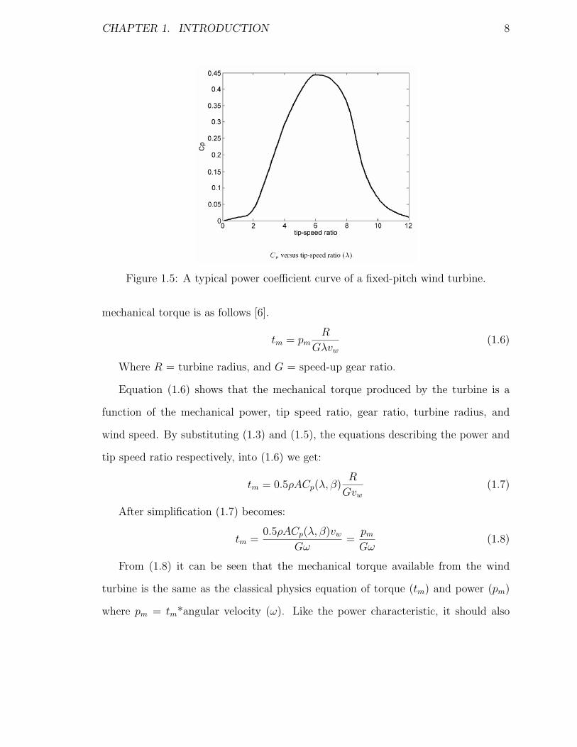
mechanical torque is as follows [6].
tm = pmR
Gλvw
(1.6)
Where R = turbine radius, and G = speed-up gear ratio.
Equation (1.6) shows that the mechanical torque produced by the turbine is a
function of the mechanical power, tip speed ratio, gear ratio, turbine radius, and
wind speed. By substituting (1.3) and (1.5), the equations describing the power and
tip speed ratio respectively, into (1.6) we get:
tm = 0.5ρACp(λ, β)R
Gvw
(1.7)
After simplification (1.7) becomes:
tm =0.5ρACp(λ, β)vw
Gω=
pm
Gω(1.8)
From (1.8) it can be seen that the mechanical torque available from the wind
turbine is the same as the classical physics equation of torque (tm) and power (pm)
where pm = tm*angular velocity (ω). Like the power characteristic, it should also
CHAPTER 1. INTRODUCTION 9
Figure 1.6: The power characteristic of a typical wind turbine (this curve illustrates(1.3)). The trajectory labelled Pmax represents the maximum points onthe power curves[3].
be noted that the shape of the torque curve is characterized by the power coefficient
(Cp). As a result, the peak torque will also correspond to a particular rotor speed.
Because the torque is the mechanical power divided by a constant gear ratio and
the angular speed of the turbine, the shape of the curve is very similar to the power
curve. Their peaks however, do not correspond to the same rotor speed. Therefore,
the rotor speed that gives maximum torque does not correspond to the rotor speed
that gives maximum power.
1.3 Concept of Maximum Power Extraction
Normal wind energy conversion is relatively straightforward process, but in order
to capture the maximum power from the wind, the process is much more involved.

CHAPTER 1. INTRODUCTION 10
It can be observed from Figure 1.6 that the maximum of the power curve, for a
particular wind speed, occurs at a particular rotor speed. Due to the aerodynamic
characteristics of a wind turbine, a small variation from the optimum rotor speed
will cause a significant decrease in the power extracted from the wind. Turbines
do not naturally operate at the optimum wind speed for any given wind velocity
because its rotor speed is dependent on the generator loading as well as the wind
speed fluctuations. Because of this, non-optimized conversion strategies lead to a
large percentage of wasted wind power. The more energy extracted from the wind,
the more cost effective the wind energy becomes.
Due to the aerodynamics of a wind turbine (dictated by the Cp function), the
same turbine angular speed for different wind speeds will result in different levels of
extracted power. Recall from Section 1.2 that the Cp,max for a fixed pitched wind
turbine corresponds to one particular TSR value (See Figure 1.5). Because the TSR
is a ratio of the wind speed and the turbine angular rotational speed, the optimum
speed for maximum power extraction is different for each wind speed [6][13], but the
optimum TSR value remains the same. As an example, figure 1.7 and 1.8 are the
power and torque characteristics of the wind turbine used in this study. The power
and torque characteristics illustrated by Figure 1.7 and Figure 1.8 are similar to the
characteristics of typical fixed pitch wind turbines. Fixed-speed wind turbine systems
will only operate at its optimum point for one wind speed [14]. So to maximize
the amount of power captured by the turbine, variable-speed wind turbine systems
are used because they allow turbine speed variation [6][14][7][3][15][16][17]. Power
extraction strategies assesses the wind conditions and then forces the system to adjust
the turbine’s rotational speed through power electronic control and/or mechanical
CHAPTER 1. INTRODUCTION 11
devices so that it will operate at the turbine’s highest aerodynamic efficiency. The
primary challenge of wind energy systems is to be able to capture as much energy
as possible from the wind in the shortest time. From the electronics point of view,
this goal can be achieved through different converter topologies and maximum power
point tracking (MPPT) algorithms.
Figure 1.7: Example: The power characteristic of the wind turbine used in this study.
1.4 Concept of Proposed Algorithm
The proposed algorithm in this thesis takes an initial guess for the optimum TSR
and subsequently uses it to calculate the starting reference signal. The system is then
adjusted towards the optimum point by using a modified version of HCS (hill climb
searching). Once an optimum point has been determined, it is stored and used when
the corresponding wind speed occurs again to speed up the determination process.
The algorithm also automatically determines a more accurate tip speed ratio for the
CHAPTER 1. INTRODUCTION 12
Figure 1.8: Example: The torque characteristic of the wind turbine used in this study.
turbine each time an optimum point is found. The establishment of the determined
tip speed ratio facilitates more accurate estimations of the optimum operating point
for wind speeds that have not yet occurred. The algorithm requires the turbine blade
radius and gear ratio, but they are easy to obtain parameters so it can be easily
configured to adapt to any turbine. These features of the proposed algorithm allow
it to be fast, effective, and flexible.
1.5 Organization of Thesis
The organization of this thesis is outlined as follows:
Chapter 1 provided some general background information regarding the motiva-
tions for wind energy research, basic wind energy conversion principles, and the basic
idea behind maximum wind power extraction. The general concept of the proposed
maximum power extraction algorithm was also presented.

CHAPTER 1. INTRODUCTION 13
Chapter 2 gives an overview of wind turbine technology and wind energy con-
version system configurations. The advantages and disadvantages of the different
types of wind turbines and the two main kinds of wind energy systems are discussed.
Power electronic interfaces and the roles of the converters are examined in this chap-
ter. Lastly, a literature review of existing maximum power point tracking techniques
is presented along with their strengths and weaknesses.
Chapter 3 describes the proposed maximum power point tracking control algo-
rithm in detail. The algorithm features, overall concept, structure and implementa-
tion are discussed.
Chapter 4 discusses the modelling of each component in the wind energy conver-
sion system considered in this thesis. The turbine model, turbine-generator shaft,
and the boost converter design are described in this chapter. This chapter also deals
with the boost converter stability analysis and the compensator design for the closed
loop verification for the proposed algorithm.
Chapter 5 uses the simulated wind energy system to systematically verify the
algorithm’s functionality. The algorithm was subjected to through various wind con-
ditions in order to confirm the effectiveness of the proposed control method.
Chapter 6 summarizes all the features ad contributions of the proposed maximum
power point tracking algorithm. It also provides suggestions on the future works that
can be done.

Chapter 2
Wind Energy Conversion Systems
2.1 Wind Turbine Technology
The wind turbine is the first and foremost element of wind power systems. There are
two main types of wind turbines, the horizontal-axis and vertical-axis turbines.
2.1.1 Horizontal-axis Turbines
Horizontal-axis turbines (see Figure 2.1) are primarily composed of a tower and a
nacelle mounted on top of tower. The generator and gearbox are normally located in
the nacelle. It has a high wind energy conversion efficiency, self-starting capability,
and access to stronger winds due to its elevation from the tower. Its disadvantages, on
the other hand, include high installation cost, the need of a strong tower to support
the nacelle and rotor blade, and longer cables to connect the top of the tower to the
ground [9].
14
CHAPTER 2. WIND ENERGY CONVERSION SYSTEMS 15
Figure 2.1: illustration of a horizontal axis and a vertical axis wind turbine [4].
2.1.2 Vertical-axis Turbines
A vertical axis turbines’ spin axis is perpendicular to the ground (See Figure 2.1) [9].
The wind turbine is vertically mounted, and its generator and gearbox is located at its
base [9]. Compared to horizontal-axis turbines, it has reduced installation cost, and
maintenance is easier, because of the ground level gear box and generator installation
[18]. Another advantage of the vertical axis turbine is that its operation is independent
of wind direction [18]. The blades and its attachments in vertical axis turbines are
also lower in cost and more rugged during operation. However, one major drawback of
the vertical wind turbine is that it has low wind energy conversion efficiency and there
are limited options for speed regulation in high winds [9]. Its efficiency is around half
of the efficiency of horizontal axis wind turbines [9]. Vertical axis turbines also have
high torque fluctuations with each revolution, and are not self-starting [9]. Mainly

CHAPTER 2. WIND ENERGY CONVERSION SYSTEMS 16
due to efficiency issue, horizontal wind turbines are primarily used. Consequently,
the wind turbine considered in this thesis is a horizontal axis turbine.
2.2 Types of Horizontal-Axis Wind Turbines
2.2.1 Pitched Controlled Wind Turbines
Pitch controlled wind turbines change the orientation of the rotor blades along its
longitudinal axis to control the output power. These turbines have controllers to
check the output power several times per second, and when the output power reaches
a maximum threshold, an order is sent to the blade hydraulic pitch mechanism of the
turbine to pitch (or to turn) the rotor slightly out of wind to slow down the turbine.
Conversely, when the wind slows down, then the blades are turned (or also known as
pitched) back into the wind. During operation, the blades are pitched a few degrees
with each change in wind to keep the rotor blades at the optimum angle to maximum
power capture. [12]
2.2.2 Stalled Controlled Wind Turbines
The rotor blades of a stall controlled wind turbine are bolted onto the hub at a fixed
angle. The blades are aerodynamically designed to slow down the blades when winds
are too strong. The stall phenomenon caused by turbulence on rotor blade prevents
the lifting force to act on the rotor. The rotor blades are twisted slightly along the
longitudinal axis so that the rotor blade stalls gradually rather than suddenly when
the wind reaches the turbines’ critical value.[12]
CHAPTER 2. WIND ENERGY CONVERSION SYSTEMS 17
2.2.3 Active Stall Controlled Wind Turbines
Active stall turbines are very similar to the pitch controlled turbine because they
operate the same way at low wind speeds. However, once the machine has reached
its rated power, active stall turbines will turn its blades in the opposite direction
from what a pitch controlled machine would. By doing this, the blades induces stall
on its rotor blades and consequently waste the excess energy in the wind to prevent
the generator from being overloaded. This mechanism is usually either realized by
hydraulic systems or electric stepper motors. [12]
2.3 Types of Wind Energy Conversion Systems
(WECS)
There are two main types of WECSs, the fixed speed WECS and variable-speed
WECS. The rotor speed of a fixed-speed WECS, also known as the Danish concept,
is fixed to a particular speed. The other type is the variable-speed WECS where the
rotor is allowed to rotate freely. The variable-speed WECS uses power maximization
techniques and algorithms to extract as much power as possible from the wind.
2.3.1 Fixed Speed Wind Energy Conversion Systems
As the name suggests, fixed speed wind energy systems operate at a constant speed.
The fixed speed WECS configuration is also known as the ”Danish concept” as it is
widely used and developed in Denmark [19]. Normally, induction (or asynchronous)
generators are used in fixed speed WECSs because of its inherent insensitivity to
changes in torque [2] [12]. The rotational speed of an induction machine varies with
CHAPTER 2. WIND ENERGY CONVERSION SYSTEMS 18
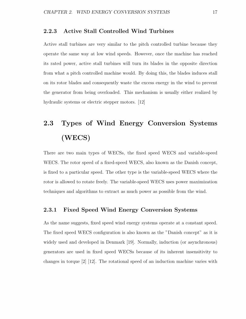
Figure 2.2: A typical fixed speed wind turbine configuration [5].
the force applied to it, but in practice, the difference between its speed at peak
power and at idle mode (at synchronous speed) is very small [2]. The fixed speed
wind systems have the generator stator directly coupled to the grid (see Figure 2.2).
Consequentially, the system is characterized by stiff power train dynamics that only
allow small variations in the rotor speed around the synchronous speed. Due to the
mechanical characteristics of the induction generator and its insensitivity to changes
in torque, the rotor speed is fixed at a particular speed dictated by the grid frequency,
regardless of the wind speed [19]. The construction and performance of fixed-speed
wind turbines are dependent on the turbine’s mechanical characteristic [14].
Squirrel-cage induction generators (SCIG) are typically used in fixed speed sys-
tems [19] [20]. The system in Figure 2.2 transforms wind energy into electrical energy
by using a squirrel cage induction machine directly connected to a three-phase power
grid [5]. The rotor of the wind turbine is coupled to the generator shaft with a fixed
ratio gearbox [5].

CHAPTER 2. WIND ENERGY CONVERSION SYSTEMS 19
With respect to variable speed wind turbines, fixed speed turbines are well es-
tablished, simple, robust, reliable, cheaper, and maintenance-free [9] [19] [20]. But
because the system is fixed at a particular speed, variation in wind speed will cause
the turbine to generate highly fluctuating output power to the grid [6], [9]. These load
variations require a stiff power grid to enable stable operation and the mechanical
design must be robust enough to absorb high mechanical stresses [5] [20]. Also, since
the turbine rotates at a fixed speed, maximum wind energy conversion efficiency can
be only achieved at one particular wind speed [6], [9]. This is because for each wind
speed, there is a particular rotor speed that will produce the TSR that gives the max-
imum Cp value. As observed from the relationship described by (1) and illustrated by
Figures 1.5 and 1.6, the maximum Cp value corresponds to the maximum mechanical
power. Since fixed speed systems do not allow significant variations in rotor speed,
these systems are incapable of achieving the various rotor speeds that result in the
maximum Cp value under varying wind conditions.
2.3.2 Variable Speed Wind Turbine Systems
In variable speed wind turbine systems, the turbine is not directly connected to the
utility grid. Instead, a power electronic interface is placed between the generator and
the grid to provide decoupling and control of the system. Thus, the turbine is allowed
to rotate at any speed over a wide range of wind speeds [6], [9]. It has been discussed
earlier that each wind speed has a corresponding optimal rotor speed for maximum
power. With the added control feature of variable speed systems, they are capable of
achieving maximum aerodynamic efficiency [9]. By using control algorithms and/or
mechanical control schemes (i.e. pitch controlled, etc), the turbine can programmed
CHAPTER 2. WIND ENERGY CONVERSION SYSTEMS 20
to extract maximum power from any wind speed by adjusting its operating point
to achieve the TSR for maximum power capture. The mechanical stresses on the
wind turbine are reduced since gusts of wind can be absorbed (i.e. energy is stored
in the mechanical inertia of the turbine and thus reduces torque pulsations) [6], [9],
[5]. Another advantage of this system is that the power quality can be improved by
the reduction of power pulsations due to its elasticity [6], [5]. The disadvantages of
the variable speed system include the additional cost of power converters and the
complexity of the control algorithms [6], [9]. In this thesis, an adaptive maximum
power point tracking control algorithm is developed for variable speed energy systems
to achieve maximum efficiency under fluctuating wind conditions.
2.4 Configurations of Variable Speed Wind Con-
version Systems
2.4.1 Synchronous Generators
The stator of the synchronous generators holds the set of three-phase windings that
supply the external load. The rotor, on the other hand, is the source of the machine’s
magnetic field. The magnetic field is either supplied by a direct current (DC) flowing
in a wound field or a permanent magnet.
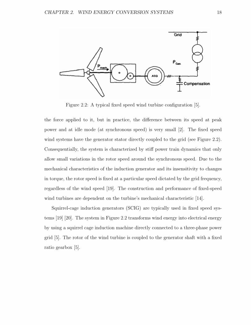
Figure 2.3 illustrates a typical setup of a wind turbine with a wound field syn-
chronous generator (WFSG) connected to the grid through power electronic convert-
ers. The WFSG has high machine efficiency, and the power electronic converters
allow direct control over the power factor. However, because of the winding circuit in
CHAPTER 2. WIND ENERGY CONVERSION SYSTEMS 21
the rotor, the size of the WFSG can be rather large. Another drawback of the con-
figuration in Figure 2.3 is that in order to regulate the active and reactive power, the
power electronic converter must be sized typically 1.2 times the rated power. Thus,
the use of the WFSG leads to a bulky system. [6]
Figure 2.3: A typical fixed speed wind turbine configuration [5].
In Figure 2.3, the stator of the turbine is connected to the utility grid through two
back-to-back pulse width modulated (PWM) converters. The main task of the stator
side converters is to control the electromagnetic torque of the turbine. By adjusting
the electromagnetic torque, the turbine can be forced to extract maximum power. The
rectifier connects the rotor and the utility; it converts the alternating current (AC)
from the utility grid into a direct current into the rotor windings. DC current flows
through the rotor windings and supplies the generator with the necessary magnetic
field for operation.
Permanent magnet synchronous generators (PMSG) are common in low power,
variable speed wind energy conversion systems [11]. The advantages of using PMSGs
are its high efficiency and small size. However, the cost of the permanent magnet
CHAPTER 2. WIND ENERGY CONVERSION SYSTEMS 22
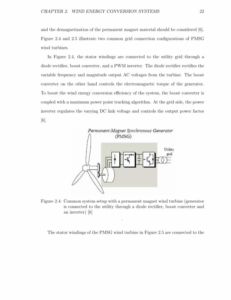
and the demagnetization of the permanent magnet material should be considered [6].
Figure 2.4 and 2.5 illustrate two common grid connection configurations of PMSG
wind turbines.
In Figure 2.4, the stator windings are connected to the utility grid through a
diode rectifier, boost converter, and a PWM inverter. The diode rectifier rectifies the
variable frequency and magnitude output AC voltages from the turbine. The boost
converter on the other hand controls the electromagnetic torque of the generator.
To boost the wind energy conversion efficiency of the system, the boost converter is
coupled with a maximum power point tracking algorithm. At the grid side, the power
inverter regulates the varying DC link voltage and controls the output power factor
[6].
Figure 2.4: Common system setup with a permanent magnet wind turbine (generatoris connected to the utility through a diode rectifier, boost converter andan inverter) [6]
.
The stator windings of the PMSG wind turbine in Figure 2.5 are connected to the
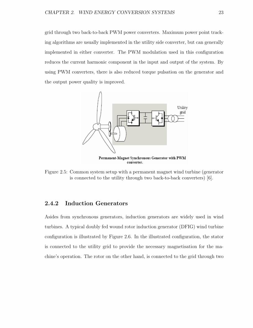
CHAPTER 2. WIND ENERGY CONVERSION SYSTEMS 23
grid through two back-to-back PWM power converters. Maximum power point track-
ing algorithms are usually implemented in the utility side converter, but can generally
implemented in either converter. The PWM modulation used in this configuration
reduces the current harmonic component in the input and output of the system. By
using PWM converters, there is also reduced torque pulsation on the generator and
the output power quality is improved.
Figure 2.5: Common system setup with a permanent magnet wind turbine (generatoris connected to the utility through two back-to-back converters) [6].
2.4.2 Induction Generators
Asides from synchronous generators, induction generators are widely used in wind
turbines. A typical doubly fed wound rotor induction generator (DFIG) wind turbine
configuration is illustrated by Figure 2.6. In the illustrated configuration, the stator
is connected to the utility grid to provide the necessary magnetisation for the ma-
chine’s operation. The rotor on the other hand, is connected to the grid through two

CHAPTER 2. WIND ENERGY CONVERSION SYSTEMS 24
Figure 2.6: Common system setup with a doubly fed wound rotor induction windturbine (the generator rotor is connected to the utility through two back-to-back converters, and the stator is connected directly to the utility)[6].
back-to-back PWM power converters. The rotor side converter regulates the electro-
magnetic torque and supplies some of the reactive power. To enable regulation of the
electromagnetic torque, algorithms for extracting maximum power are implemented
in the rotor side converter stage. The controller of the utility side converter regulates
the voltage across the DC link for power transmission to the gird. There are reduced
inverter costs associated with the DFIG wind turbine because the power converters
only need to control the slip power of the rotor. Another advantage of the DFIG is
its two degrees of freedom; the power flow can be regulated between the two wind
systems (rotor and stator) [21]. This feature allows minimization of losses associated
with a given operating point as well as other performance enhancements [21]. A dis-
advantage for using the DFIG wind turbine, however, is that the generator uses slip
rings. Since slip rings must be replaced periodically, and so the use of DFIGs trans-
lates to more frequent maintenance issues and long term costs than other brushless
generators. [6]

CHAPTER 2. WIND ENERGY CONVERSION SYSTEMS 25
The stator of the squirrel cage induction generator (SCIG) in Figure 2.7 is con-
nected to the grid through two back-to-back PWM converters. The stator side con-
verter regulates the electromagnetic torque and supplies the necessary reactive power
to magnetize the machine. The grid side converter on the other hand controls the
power quality generated power to the grid. It accomplishes this task by regulating the
real and reactive power delivered to the grid while regulating the (direct current) DC
link voltage. The squirrel cage induction machine is very rugged, brushless, reliable,
and cost effective. However, the drawback of using the SCIG is that the stator side
converter must be oversized by 30-50% of machine’s rated power in order to be able to
satisfy the machine’s magnetizing requirement. Therefore, although the SCIG itself is
cost effective, the necessary power converters for its control are relatively more bulky
and expensive. [6]
Figure 2.7: Common system setup with a squirrel cage induction generator (generatoris connected to the utility through two back-to-back converters) [6].

CHAPTER 2. WIND ENERGY CONVERSION SYSTEMS 26
2.5 Literature Review of Maximum Power Extrac-
tion Techniques
Since wind availability is sporadic and unpredictable, it is desirable to develop fast
and efficient methods to track the optimal operation points of a variable speed wind
energy system (WES). Many methods have been proposed and discussed in literature
[13][7], [17][22][23]. This section will discuss methods that pertain to variable speed
wind energy systems that use the PMSG generator.
The methods in [13] are based on the principle of loading the wind turbine to en-
sure that the maximum available energy from the wind is extracted. The two meth-
ods in [13] utilize the turbine characteristics (torque, power and power coefficient
curves) to determine the operating point that results in maximum power capture.
The only difference between the two methods presented in [13] is that one requires
an anemometer so that the wind speed is physically measured while and the second
method calculates the wind speed using electrical parameters. These methods are
advantageous for fast optimum point determination and easy implementation since
all the physical characteristics of the turbine are programmed directly and optimum
operation point is determined by simply examining the characteristics. A disadvan-
tage of these strategies however, is that they are customized for a particular turbine.
In another words, if these strategies are to be used, they will need to be programmed
with the turbine characteristics for the particular turbine in question. Another draw-
back of this algorithm is that it cannot take into account the atmospheric changes
in air density, since for all its calculations, it assumes a certain value. The air den-
sity plays a significant part in the aerodynamics of the turbine, and thus affects the

CHAPTER 2. WIND ENERGY CONVERSION SYSTEMS 27
accuracy of the pre-programmed turbine characteristics.
A maximum power point algorithm is proposed in [23] uses a maximum-efficiency
control and a maximum-torque control to maximize the turbine output power. Based
on the turbine characteristics of a selected turbine, the relationship between the op-
timum generator torque and the generator speed is established. This relationship
determines the behaviour of the maximum-torque control. For any particular wind
speed the generator torque balances the mechanical torque so that they will be equiv-
alent at the optimum operating point. Since the generator torque is controlled in
such a way that it tracks the optimum torque curve. An advantage of this method is
that it does not require a wind speed detector. A drawback of this method is that to
select the proportional constant that describes the relationship between the generator
torque and speed is based on the turbine characteristics. This dependency hinders
its ability to be used for various wind turbines, since different turbines have different
characteristics.
The method in [7] is an Advanced Hill Climb Search (AHCS) that maximizes the
power by detecting the inverter output power (Pout) and the inverter dc-link voltage.
In their wind energy conversion system, they use a diode rectifier to first convert the
three-phase output ac voltage from the generator to a dc voltage (Vdc). Vdc is related
to the generator angular rotational speed (ω) by the generator field current (If ) and
the load current (Ig) of the PMSG: Vdc = k(If , Ig) ∗ ω [7]. The authors in [7] noted
that if the sampling period of the control system is adequately small then the term
k(If , Ig) can be considered constant. The algorithm uses the relationship between the
turbine mechanical power Pm, and the electrical system output power (Pout) given by
(2.1). By differentiating (2.1) to get a relationship for ∆Pm, equation 2.2 is obtained.

CHAPTER 2. WIND ENERGY CONVERSION SYSTEMS 28
Pm = PLoad + Tf ∗ ω + ω ∗ Jdω
dt=
1
νPout + Tf ∗ ω + ω ∗ J
dω
dt(2.1)
∆Pm =1
ν∆Pout + Tf ∗ ∆ω + ∆(ω ∗ J
dω
dt) (2.2)
In order to establish rules to adjust the system’s operating point, this method
evaluates the values of ∆Pout and ∆(Vdc ∗ dVdc/dt) (which represents ∆(ω ∗ dω/dt))
based on (2.2). Depending on the values of ∆Pout and ∆(Vdc ∗ dVdc/dt) the polarity
of the inverter current demand control signal (Idm) is decided. There are three basic
modes for this method, i) initial mode, ii) training mode, and iii) application mode.
During its initial mode, before the algorithm has been trained, the magnitude of Idm
is determined by the max-power error driven (MPED) control. MPED control is the
implementation of the conventional hill climb search (HCS) method in terms of wind
energy system characteristics. During its training mode, the algorithm continually
records and updates operating parameters into its programmable lookup table for
its intelligent memory feature. Since this method is trainable with its intelligent
memory, it allows itself to adapt to a turbine. As a result, it is a solution to the
customization problems of many algorithms. Another advantage of this algorithm
is that does not require mechanical sensors (like anemometers) which lowers its cost
and eliminates its associated practical issues. However, it can be seen in [7] that the
algorithm is relatively slow and complex as it has three different modes of operation.
Another drawback is that the algorithm cannot take into account of the changes in air
density, which affects the power characteristics quite significantly [17] (see Figure 2.8).
Its lookup table updating process will be adversely affected due fluctuations in air
density. The updating method in [7] states that the lookup table, which constitutes
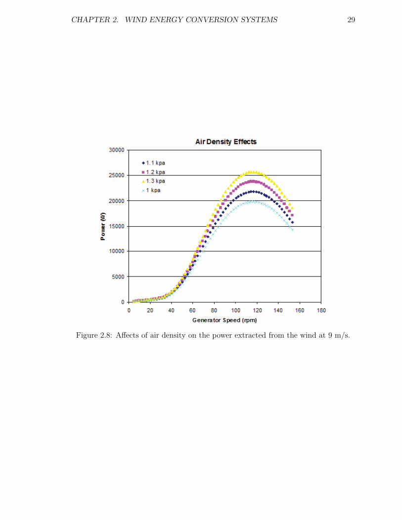
CHAPTER 2. WIND ENERGY CONVERSION SYSTEMS 29
Figure 2.8: Affects of air density on the power extracted from the wind at 9 m/s.
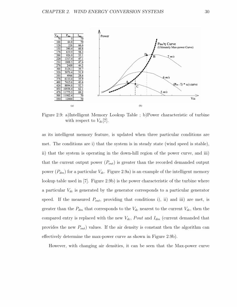
CHAPTER 2. WIND ENERGY CONVERSION SYSTEMS 30
(a) (b)
Figure 2.9: a)Intelligent Memory Lookup Table ; b)Power characteristic of turbinewith respect to Vdc[7].
as its intelligent memory feature, is updated when three particular conditions are
met. The conditions are i) that the system is in steady state (wind speed is stable),
ii) that the system is operating in the down-hill region of the power curve, and iii)
that the current output power (Pout) is greater than the recorded demanded output
power (Pdm) for a particular Vdc. Figure 2.9a) is an example of the intelligent memory
lookup table used in [7]. Figure 2.9b) is the power characteristic of the turbine where
a particular Vdc is generated by the generator corresponds to a particular generator
speed. If the measured Pout, providing that conditions i), ii) and iii) are met, is
greater than the Pdm that corresponds to the Vdc nearest to the current Vdc, then the
compared entry is replaced with the new Vdc, Pout and Idm (current demanded that
provides the new Pout) values. If the air density is constant then the algorithm can
effectively determine the max-power curve as shown in Figure 2.9b).
However, with changing air densities, it can be seen that the Max-power curve
CHAPTER 2. WIND ENERGY CONVERSION SYSTEMS 31
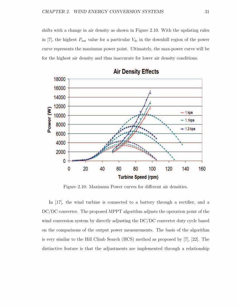
shifts with a change in air density as shown in Figure 2.10. With the updating rules
in [7], the highest Pout value for a particular Vdc in the downhill region of the power
curve represents the maximum power point. Ultimately, the max-power curve will be
for the highest air density and thus inaccurate for lower air density conditions.
Figure 2.10: Maximum Power curves for different air densities.
In [17], the wind turbine is connected to a battery through a rectifier, and a
DC/DC converter. The proposed MPPT algorithm adjusts the operation point of the
wind conversion system by directly adjusting the DC/DC converter duty cycle based
on the comparisons of the output power measurements. The basis of the algorithm
is very similar to the Hill Climb Search (HCS) method as proposed by [7], [22]. The
distinctive feature is that the adjustments are implemented through a relationship

CHAPTER 2. WIND ENERGY CONVERSION SYSTEMS 32
found between the change in output power and the duty ratio. Relationships between
the duty ratios of the buck, buck-boost, and boost converters and the change in output
power have been described in [17]. Thus, the algorithm determines the operation point
adjustment based on the change in power with respect to the duty cycle.
The proposed algorithm in [22] searches for the peak power by changing the speed
reference in the appropriate direction. Depending on the magnitude and direction of
change in active power, the speed reference is modified towards it optimal operating
point. The peak power points are identified on the power versus generator shaft speed
curve where its derivative is zero; the power curve looks similar to that of an inverse
parabola see Figure 1.7.
In [22], the output power and speed are sampled at regular intervals of time, and
if the wind velocity is stable and the system was originally at its optimum point,
then no action is taking. When there is a step change in wind velocity, the turbine is
no longer operating at its optimum point and there will be a corresponding change
in power. Positive power change corresponds to increased speed reference propor-
tional the change in power, and a negative power change corresponds to decreased
speed reference. For further adjustment (when wind speed is stable) the speed ref-
erence direction is determined by both the change in power and the previous speed
reference direction. For example, if a reduced speed reference resulted in a positive
change in power then the system will continue reduce the speed reference. When the
change in power is minimal (within a predefined limit) then no further change in the
speed reference is made (since the minimal change in power translates to the peak
power point). A disadvantage of this algorithm is that uses the turbine characteristics
(torque, power and power coefficient curves) to determine the amount of change in

CHAPTER 2. WIND ENERGY CONVERSION SYSTEMS 33
the speed reference with respect to the change in power. This introduces dependence
of the algorithm to the characteristics of a particular turbine. Another drawback of
this algorithm is that it does not have any means to store the previously determined
peak power operating points. This means that with each change in wind speed, the
algorithm will have to search for the optimum point even if it has been previously de-
termined. The repetitiveness of the searching procedure will slow down the optimum
point determination process and cause subsequent losses potential output power.
2.5.1 Summary of MPPT Algorithms
The methods in [7], [17], [22] use the changes in power (∆P ) and the changes in
generator speed (∆ω) to adjust the generator speed towards the optimum operating
point. The intelligent memory in [7] allows the algorithm to be more efficient over
time as the optimal points are stored, when determined, for later use. The methods in
[7],[17], [22] are independent of turbine characteristics, so they are flexible and can be
applied to various turbines. These algorithms, however, would be slower than those
in [13] and [23] because of their adjustment process. The algorithms described in [13]
and [23] fast and efficient, but they are dependent on having prior knowledge of the
turbine characteristics. Therefore the methods in [13] and [23] cannot be used for a
wide range of turbines and cannot consider machine degradation since they cannot
adapt to change.

Chapter 3
Proposed Algorithm
3.1 Algorithm Concept and Features
The proposed algorithm uses the HCS methodology along with intelligent memory
and power management to track the maximum power points of wind energy systems
under fluctuating wind conditions. The main problems in existing power extraction
methods are: i) customization, ii) speed, and iii) wasted power. The proposed al-
gorithm provides a solution to these problems. In order to avoid the customization
problems in some of the existing algorithms, the proposed technique does not re-
quire the characteristics of the turbine to be preprogrammed. Instead, the algorithm
initially uses a general estimate of the turbine characteristics and then determines
the actual characteristics through operation. By doing this, the algorithm can be
easily used for a wide range of wind turbines. The turbine adaptation feature of
the algorithm allows it to immediately make fairly accurate estimations on the maxi-
mum power points of the system following the determinations of the maximum power
34
CHAPTER 3. PROPOSED ALGORITHM 35
points. The estimations allow the system to immediately operate near to the maxi-
mum power point, where the change in speed corresponds to small changes in power.
Therefore, the estimations lead to less wasted potential power and speed up the de-
termination process. The closer the operating point is to the maximum power point,
the fewer adjustments necessary.
The proposed algorithm has two main concepts to enable flexible, fast and efficient
maximum power extraction. The first concept is to quickly determine the maximum
power point by using the turbine fundamental tip-speed ratio equation in conjunction
with the HCS methodology. The second concept is to enable immediate maximum
point retrieval for reoccurring wind speeds and determination of the given turbine’s
internal actual TSR. Recall that the TSR is the ratio of the wind speed and the rotor
speed, and for each turbine there is one TSR that will always result in maximum power
transfer. The TSR is characterizes the aerodynamic efficiency of a wind turbine and
is unique. Please note that the dynamic response of the generator dictates the speed
at which the algorithm can determine an optimum point. This is because the system
will not make any decisions or adjustment to the speed reference until it has reached
steady-state (i.e. reached the reference for a defined period of time).
3.1.1 Modified Hill Climb Search
Due to the nature of wind energy systems described in chapter 1, the power available
from the wind turbine is a function of both the wind speed and the rotor angular
speed. The wind speed being uncontrollable, the only way to alter the operating point
is to control the rotor speed. Rotor speed control can be achieved by using power
electronics to control the loading of the generator. Without any given knowledge of

CHAPTER 3. PROPOSED ALGORITHM 36
the aerodynamics of any wind turbine, the HCS principle searches for the maximum
power point by adjusting the operating point and observing the corresponding change
in the output. The HCS concept is essentially an ”observe and perturb” concept used
to traverse the natural power curve of the turbine. With respect to wind energy
systems, it monitors the changes in the output power of the turbine and rotor speed.
The maximum power point is defined by the power curve in Fig. 3.1 where ∆P/∆ω
= 0. Thus, the objective of HCS is to ’climb’ the curve by changing the rotor angular
speed and measuring the output power until the condition of ∆P/∆ω = 0 is met.
There are several different ways of implementing the HCS idea.
In this thesis, the algorithm generates the reference speed by measuring the output
power of the wind energy conversion system and adjusts the system’s operating point
accordingly. The ∆P/∆ω = 0 condition is achieved when ∆P ≈ 0 because the
amount of adjustment in the rotor speed is chosen to be proportional to the change
in power; thus when ∆P∆ω
≈ 0. The HCS concept is described in detail in this section
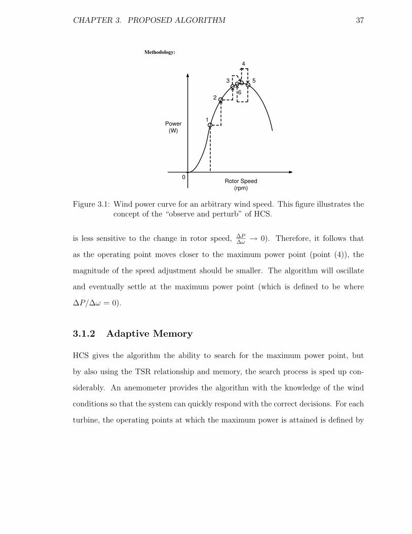
according to this thesis’ implementation method and it is illustrated by Figure 3.1.
The system begins at point 1 and chooses to increase the rotor speed to point 2.
Observing that that there has been an increase in power due to an increase in speed,
the algorithm signals to further increase the rotor speed to point 3. Since ∆P/∆ω
is positive, the system is ’climbing’ up the power curve. With ∆P/∆ω still positive,
the system continues to increase the rotor speed to point 5. The algorithm notices
that the change in power from point 4 and point 5 is negative, and it was due to an
increase in speed. With ∆P/∆ω now negative, the optimum point has been passed.
As a result, the rotor speed is decreased to point 6. The slope of the power curve
diminishes as the system approaches the peak power point (level of extracted power
CHAPTER 3. PROPOSED ALGORITHM 37
Methodology:
Rotor Speed
(rpm)
Power
(W)
0
1
2
3
4
5
6
Figure 3.1: Wind power curve for an arbitrary wind speed. This figure illustrates theconcept of the “observe and perturb” of HCS.
is less sensitive to the change in rotor speed, ∆P∆ω
→ 0). Therefore, it follows that
as the operating point moves closer to the maximum power point (point (4)), the
magnitude of the speed adjustment should be smaller. The algorithm will oscillate
and eventually settle at the maximum power point (which is defined to be where
∆P/∆ω = 0).
3.1.2 Adaptive Memory
HCS gives the algorithm the ability to search for the maximum power point, but
by also using the TSR relationship and memory, the search process is sped up con-
siderably. An anemometer provides the algorithm with the knowledge of the wind
conditions so that the system can quickly respond with the correct decisions. For each
turbine, the operating points at which the maximum power is attained is defined by

CHAPTER 3. PROPOSED ALGORITHM 38
the wind speed and its corresponding rotor speed. In order to keep the system in-
dependent from the physical characteristics of the wind turbine, and thus keeping it
easily modifiable to other turbines, an approximate “optimal” TSR is used initially.
The memory feature of this algorithm not only allows immediate access to the
maximum power points previously determined, it also enables the algorithm to adapt
to its given turbine. The adaptability of the algorithm allows the system to capture
as much available power as possible under fast wind variations. The memory provides
two major power management functions; i) store the operating points as determined
by the algorithm, ii) to update the approximate TSR to a value nearer to the actual
TSR.
The algorithm stores the determined operating points with respect to the wind
speed. This allows the system to immediately jump to the optimal operating point,
thereby bypassing the time-consuming searching procedure. In the case that the
stored operating point is not ideal, after the determined maximum power point is
reached, small adjustments are made to ensure the integrity of the stored data. With
small adjustments, minimal power is wasted during this process because the system
will be operating very close to its maximum efficiency.
With each successful determination of a maximum power point, the data is used to
obtain a more accurate TSR using (1.5). Since it is known that the maximum power
point for a particular turbine always occurs at the same optimal TSR for all wind
speeds, the TSR is updated to be the average TSR obtained from each data entry.
As a result, each time a new wind speed occurs, the approximate operating point,
using the updated TSR, will become closer and closer to the actual maximum power
point. Thus, the searching process is continuously shortened with each optimum point
CHAPTER 3. PROPOSED ALGORITHM 39
determination.
3.1.3 Algorithm Structure
Figure 3.2, 3.3, and 3.4, illustrate the different stages of the proposed algorithm logic.
It is necessary to note that all measurements and adjustments are made after the
system is steady at its current operating point. This prevents incorrect decision due
to transient fluctuations.
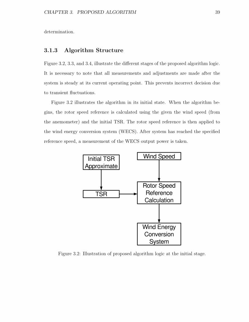
Figure 3.2 illustrates the algorithm in its initial state. When the algorithm be-
gins, the rotor speed reference is calculated using the given the wind speed (from
the anemometer) and the initial TSR. The rotor speed reference is then applied to
the wind energy conversion system (WECS). After system has reached the specified
reference speed, a measurement of the WECS output power is taken.
Wind Speed
Rotor Speed
Reference Calculation
TSR
Initial TSR Approximate
Wind Energy Conversion
System
Figure 3.2: Illustration of proposed algorithm logic at the initial stage.
CHAPTER 3. PROPOSED ALGORITHM 40
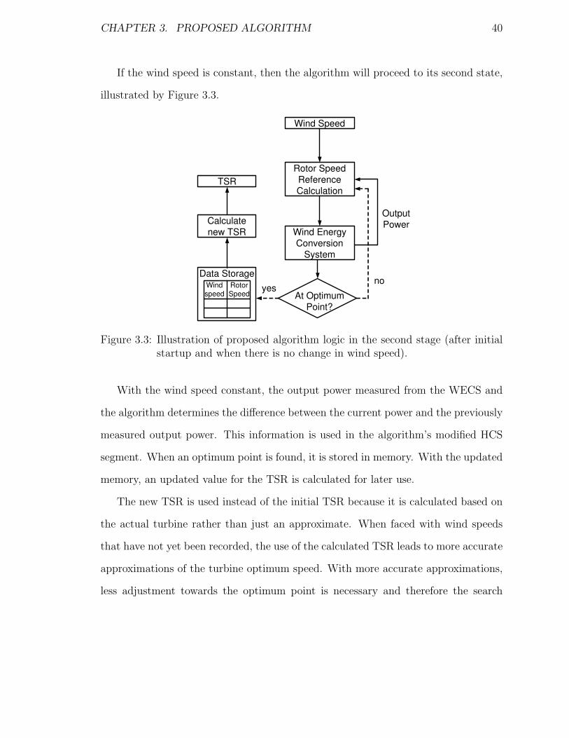
If the wind speed is constant, then the algorithm will proceed to its second state,
illustrated by Figure 3.3.
Wind Speed
Rotor Speed
Reference
CalculationTSR
Wind Energy
Conversion
System
Output
Power
At Optimum
Point?
Calculate
new TSR
Data StorageWindspeed
RotorSpeed
yesno
Figure 3.3: Illustration of proposed algorithm logic in the second stage (after initialstartup and when there is no change in wind speed).
With the wind speed constant, the output power measured from the WECS and
the algorithm determines the difference between the current power and the previously
measured output power. This information is used in the algorithm’s modified HCS
segment. When an optimum point is found, it is stored in memory. With the updated
memory, an updated value for the TSR is calculated for later use.
The new TSR is used instead of the initial TSR because it is calculated based on
the actual turbine rather than just an approximate. When faced with wind speeds
that have not yet been recorded, the use of the calculated TSR leads to more accurate
approximations of the turbine optimum speed. With more accurate approximations,
less adjustment towards the optimum point is necessary and therefore the search
CHAPTER 3. PROPOSED ALGORITHM 41
process is further sped up.
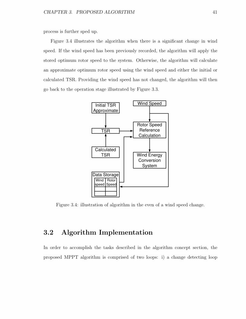
Figure 3.4 illustrates the algorithm when there is a significant change in wind
speed. If the wind speed has been previously recorded, the algorithm will apply the
stored optimum rotor speed to the system. Otherwise, the algorithm will calculate
an approximate optimum rotor speed using the wind speed and either the initial or
calculated TSR. Providing the wind speed has not changed, the algorithm will then
go back to the operation stage illustrated by Figure 3.3.
Wind Speed
Rotor Speed
Reference
CalculationTSR
Initial TSR
Approximate
Wind Energy
Conversion
System
Calculated
TSR
Data StorageWindspeed
RotorSpeed
Figure 3.4: illustration of algorithm in the even of a wind speed change.
3.2 Algorithm Implementation
In order to accomplish the tasks described in the algorithm concept section, the
proposed MPPT algorithm is comprised of two loops: i) a change detecting loop
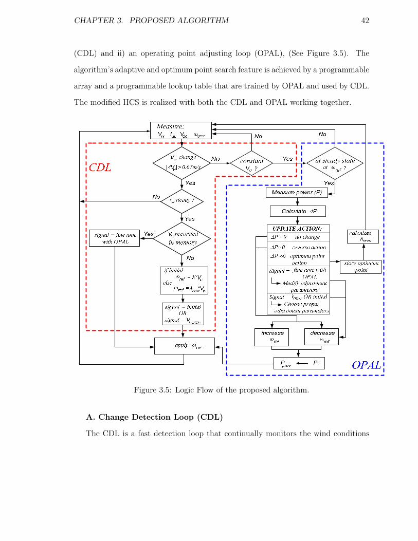
CHAPTER 3. PROPOSED ALGORITHM 42
(CDL) and ii) an operating point adjusting loop (OPAL), (See Figure 3.5). The
algorithm’s adaptive and optimum point search feature is achieved by a programmable
array and a programmable lookup table that are trained by OPAL and used by CDL.
The modified HCS is realized with both the CDL and OPAL working together.
Figure 3.5: Logic Flow of the proposed algorithm.
A. Change Detection Loop (CDL)
The CDL is a fast detection loop that continually monitors the wind conditions

CHAPTER 3. PROPOSED ALGORITHM 43
and executes the actions necessary to efficiently determine the optimum point while
minimizing the loss of potential wind energy. Whenever the system is not operating
at its ideal operating point for a particular wind velocity, the amount of potential
wind energy lost can be quite significant. Therefore, the speed of the CDL is crucial
to manage the algorithm so that incorrect decisions due to the fluctuations in the
wind can be immediately corrected. CDL is executed initially and whenever a change
in wind speed is detected. When a wind speed change has been detected, then it will
initiate the execution of OPAL, determine an approximate maximum power point, or
search for a previously recorded optimum power point.
Upon startup, the algorithm calculates an initial reference speed, ωref , by using
(1.3), where λ = 7. This value of the tip-speed ratio is a generic λopt for a 3-blade wind
turbine as suggested by [24]. The selected initial value for the TSR is not optimal,
so the calculated speed reference will not be the optimal point. However, by using
the suggested value of an optimal TSR for a generic turbine, it allows the system to
begin at an operating point near the actual maximum power point rather than at an
arbitrary point.
The algorithm is programmed in C++ through the power simulator program
(PSIM). Since wind is always constantly fluctuating, a wind speed is considered steady
when the changes are within ±0.07 m/s (0.252 km/h). To detect this, the fast CDL
loop measures the current wind speed, vw(n), and compares to the previous stored
value, vw(n − 1). If the difference, vw, is within the specified range to be considered
constant for a specified amount of time, then no further action is taken by CDL and
OPAL will be executed. However, if | vw | is greater than the specified threshold, CDL
will search through the lookup table (programmed by OPAL) to see if the current

CHAPTER 3. PROPOSED ALGORITHM 44
wind speed is within ±0.07 m/s of any recorded wind speed.
If a stored wind speed within ±0.07 m/s of the current wind speed is found,
then the corresponding recorded ωopt is used as the reference speed and OPAL will
be signaled to make minor adjustments to ensure the integrity of the stored data.
Since each optimum point is determined through operation it may not be the exact
optimum power point, instead it will be an operating point that is extremely close
to the maximum power point. To further move the operating point closer to the
actual maximum power point rather than deviating, small adjustments are made to
ensure that the applied speed reference is the maximum point. In the case that it is
not as optimal, the small adjustments will fine tune the stored maximum operating
point to its true value. Due to the flat-topped nature of wind power curves, small
adjustments around the maximum power point will not result in much loss of potential
wind power. The immediate use of a stored optimal speed allows the algorithm to
eliminate any redundant searches that have been done before. Standard HCS will
always go through the full search each time the wind speed changes and causes it to
be slower and therefore more potential energy is wasted.
In the case that the current wind speed is not within ±0.07m/s of any stored
wind speed in the database, then ωref is calculated with either the updated λnew
(determined by OPAL) or the initial λ, and OPAL will be signaled to be executed to
adjust ωref towards the optimum point.
B. Operation Point Adjusting Loop (OPAL)
This process is executed when it is signaled by CDL. Its main task is to adjust the
system’s operating point towards the optimum generator speed, ωopt, using a modified
hill climb search (HCS) method and to train the adaptive memory.

CHAPTER 3. PROPOSED ALGORITHM 45
OPAL determines whether the generator should be sped up or slowed down de-
pending on ∆P , system status, and the change in speed reference based on a modified
HCS principle (See Table 1 for the modified HCS decision parameters). Thus, de-
pending on the decision parameters, ωref is adjusted accordingly towards ωopt. To
avoid unnecessary computations that cause the system to take a longer time to find
the optimum point (due to incorrect decisions), no adjustment to ωref is made until
the system has reached steady state at the current ωref .
The adaptive feature is realized by a programmable look up table and a pro-
grammable array that are trained by updating it whenever a ωopt is determined for
a new wind speed. The look up table is updated by storing the determined ωopt and
its corresponding wind speed into memory. The array, on the other hand, is updated
by storing the calculated λopt from the ωopt and wind speed values. The average of
the recorded λ values in the array then becomes λnew (an approximate of the actual
λopt) for the next CDL iteration. The optimum point determination process is sped
up by the adaptive feature as the look up table allows the system to immediately
obtain the ωopt for a reoccurring wind speed. The array also speeds up the process
by allowing the CDL to obtain a fairly accurate ωref so that minimal adjustment by
OPAL is required.
B.1 Modified Hill Climb Search
The concept behind the modified HCS method is to determine the power change
(∆P ) with respect to the change in rotor speed while using the TSR and memory to
jump to an operating point closer to the maximum power point. Unlike the standard
HCS method, the proposed algorithm’s TSR concept and memory guarantees the
system to immediately begin at a point relatively close the maximum power point
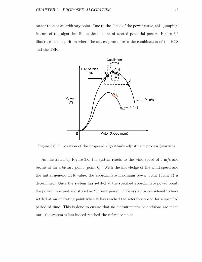
CHAPTER 3. PROPOSED ALGORITHM 46
rather than at an arbitrary point. Due to the shape of the power curve, this ’jumping’
feature of the algorithm limits the amount of wasted potential power. Figure 3.6
illustrates the algorithm where the search procedure is the combination of the HCS
and the TSR.
Figure 3.6: Illustration of the proposed algorithm’s adjustment process (startup).
As illustrated by Figure 3.6, the system reacts to the wind speed of 9 m/s and
begins at an arbitrary point (point 0). With the knowledge of the wind speed and
the initial generic TSR value, the approximate maximum power point (point 1) is
determined. Once the system has settled at the specified approximate power point,
the power measured and stored as “current power”. The system is considered to have
settled at an operating point when it has reached the reference speed for a specified
period of time. This is done to ensure that no measurements or decisions are made
until the system is has indeed reached the reference point.

CHAPTER 3. PROPOSED ALGORITHM 47
Since it is during the initial startup of the algorithm, the algorithm has no knowl-
edge of any maximum power points, the turbine’s optimum TSR, or where the current
operating point lies on the power curve. As a result, the algorithm has two choices.
It can arbitrarily choose to either increase or decrease the current generator speed by
3% and observe the effects. Here, the proposed algorithm is programmed to initially
increase the rotor speed. Once the reference speed (97% of the current rotor speed)
is applied to the system, the algorithm monitors the system response. Once the algo-
rithm detects that the system has settled at the specified speed (point 2), the power
is measured. The previously measured power at point 1 is stored now as “previous
power” and the new measurement at point 2 replaces the “current power”. Noticing
an increase in power from point 1 to 2 as a result of the increase in rotor speed, the al-
gorithm continues to increase the rotor speed. Now, with data regarding the increase
in power as a result of the change in speed, the speed reference is increased by half of
the change in power, ∆P (where ∆P = current power - previous power). In addition,
because both ∆ω and ∆P are positive, the algorithm acknowledges that it is currently
operating at a point that is to the left of the maximum power point. This process
continues until the system reaches point 4. From point 3 to 4, there is a decrease
in power corresponding to the increase in speed, so the algorithm acknowledges that
the optimum power point has been passed. Consequentially, the algorithm decreases
the rotor speed proportionally to the change in power and the system. Whenever the
algorithm detects a negative change in speed, the speed reference change will reverse
in direction. As a result, the system will oscillate around and eventually settle at
the optimum point (point 5). As illustrated in Figure 3.6, because of the gradual
decrease in the change in power, as the operating point becomes nearer and nearer to

CHAPTER 3. PROPOSED ALGORITHM 48
the maximum power point, the change in rotor speed also decreases. When the ∆P is
detected to be within ±0.5% of the current power, then it is considered to be almost
zero. However, if 0.5% of the current power is more than 30W, then the specified
range where ∆P is considered zero is limited to 30W. Since ∆ω is proportional to
∆P , the maximum power point (∆P/∆ω = 0) is reached when ∆P = ±0.5% of the
current power or (±30W ). Once the maximum power point has been reached, the
wind speed and current speed is recorded into the memory. The data is then used to
calculate the optimal TSR for the specified turbine to replace the initial generic TSR
value.
Due to a change in wind to 7 m/s after the maximum power point has been de-
termined for 9 m/s, the operating point shifts to point 6. Because of the inertial
properties and the system’s mechanical time constant, the system speed does not
change immediately. As a result, the system will continue to operate at its previ-
ous speed, but the operating point is no longer optimal. Figure 3.7 illustrates the
algorithm operation under a new wind condition after an operating point has been
determined.
Once a new wind speed has been detected, CDL is invoked and a new speed
reference is generated using the determined TSR value from the previous maximum
power point. Since the optimum TSR for maximum power transfer for a turbine
is the same under all wind conditions (since it is the ratio between the rotational
speed and the wind speed), the determined TSR will be valid for the new wind speed.
Therefore, the approximate optimum speed (point 8) will be very close to the actual
maximum power point. Because the operating point is so close to the actual maximum
power point, subsequent adjustments to the reference will be small to ensure that the
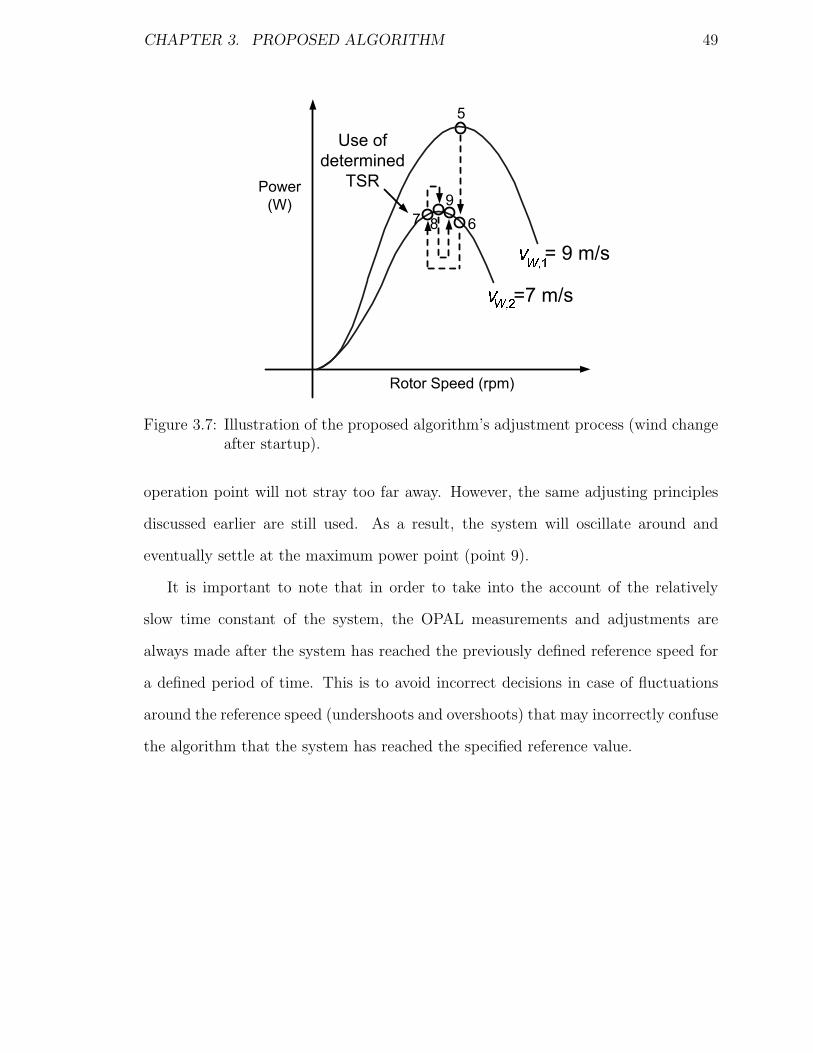
CHAPTER 3. PROPOSED ALGORITHM 49
Figure 3.7: Illustration of the proposed algorithm’s adjustment process (wind changeafter startup).
operation point will not stray too far away. However, the same adjusting principles
discussed earlier are still used. As a result, the system will oscillate around and
eventually settle at the maximum power point (point 9).
It is important to note that in order to take into the account of the relatively
slow time constant of the system, the OPAL measurements and adjustments are
always made after the system has reached the previously defined reference speed for
a defined period of time. This is to avoid incorrect decisions in case of fluctuations
around the reference speed (undershoots and overshoots) that may incorrectly confuse
the algorithm that the system has reached the specified reference value.

Chapter 4
System Modelling
The main focus of this thesis is to provide a control algorithm for wind energy systems
to extract as much power as possible from the wind, so the turbine-generator values
were chosen based on [25] to emulate a wind energy system. The most important
function of system modelling in this thesis is to ensure that the torque and power
transfer from the wind turbine to the generator relationship is correct. It suffices to
have the designed system to behave similarity to the WECS presented in literature.
The system was also modelled in such a way that effects, such as tower shadow, etc.,
were neglected so that the system can reflect the performance of the control algorithm
clearly.
The system considered in this thesis is a front-end rectifier system, where its main
purpose is to rectify the generator output voltage and control the system to shift the
system operating point to enable maximum power extraction. The WECS considered
in this thesis is illustrated in Figure 4.1. The system consists of a wind turbine,
permanent magnet synchronous machine, a diode rectifier, and a boost converter.
50
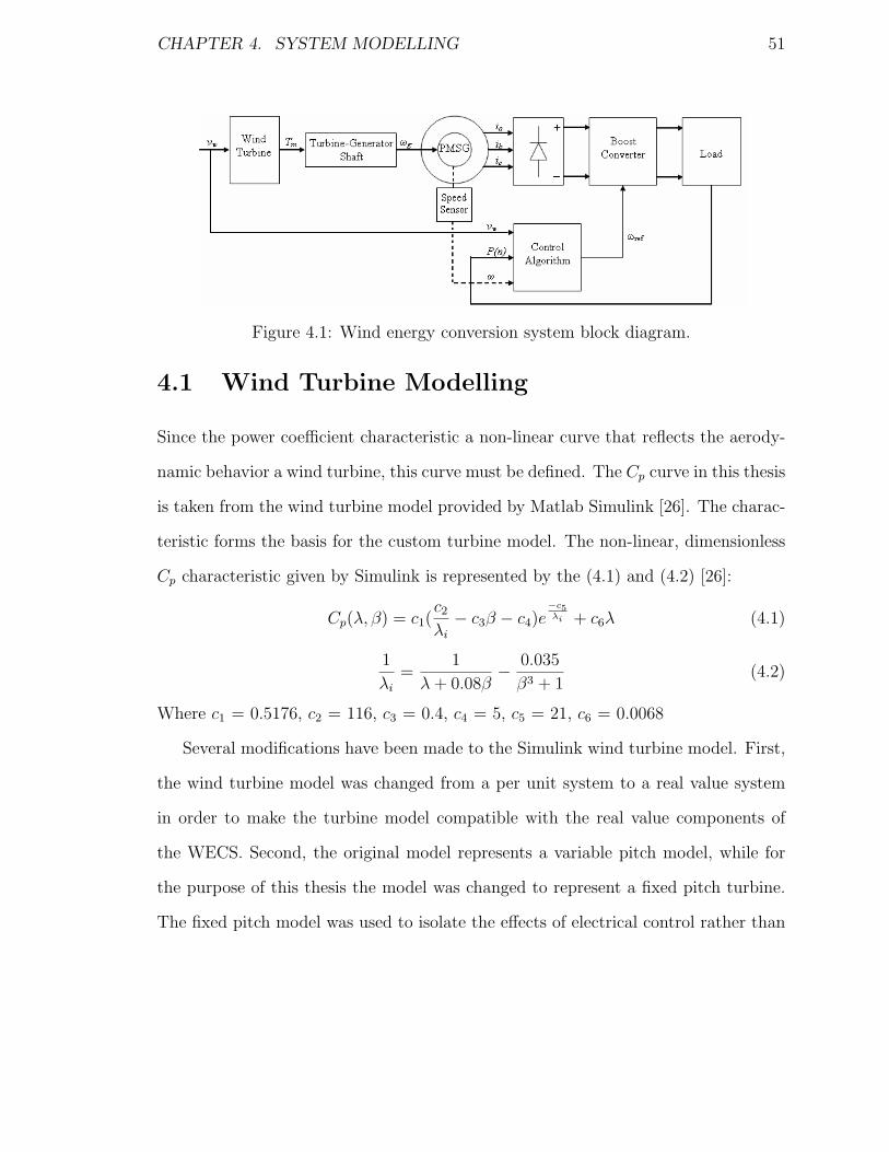
CHAPTER 4. SYSTEM MODELLING 51
Figure 4.1: Wind energy conversion system block diagram.
4.1 Wind Turbine Modelling
Since the power coefficient characteristic a non-linear curve that reflects the aerody-
namic behavior a wind turbine, this curve must be defined. The Cp curve in this thesis
is taken from the wind turbine model provided by Matlab Simulink [26]. The charac-
teristic forms the basis for the custom turbine model. The non-linear, dimensionless
Cp characteristic given by Simulink is represented by the (4.1) and (4.2) [26]:
Cp(λ, β) = c1(c2
λi
− c3β − c4)e−c5λi + c6λ (4.1)
1
λi
=1
λ + 0.08β−
0.035
β3 + 1(4.2)
Where c1 = 0.5176, c2 = 116, c3 = 0.4, c4 = 5, c5 = 21, c6 = 0.0068
Several modifications have been made to the Simulink wind turbine model. First,
the wind turbine model was changed from a per unit system to a real value system
in order to make the turbine model compatible with the real value components of
the WECS. Second, the original model represents a variable pitch model, while for
the purpose of this thesis the model was changed to represent a fixed pitch turbine.
The fixed pitch model was used to isolate the effects of electrical control rather than
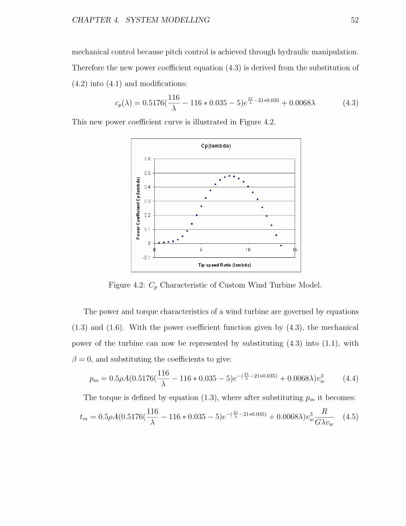
CHAPTER 4. SYSTEM MODELLING 52
mechanical control because pitch control is achieved through hydraulic manipulation.
Therefore the new power coefficient equation (4.3) is derived from the substitution of
(4.2) into (4.1) and modifications:
cp(λ) = 0.5176(116
λ− 116 ∗ 0.035 − 5)e
21
λ−21∗0.035 + 0.0068λ (4.3)
This new power coefficient curve is illustrated in Figure 4.2.
Figure 4.2: Cp Characteristic of Custom Wind Turbine Model.
The power and torque characteristics of a wind turbine are governed by equations
(1.3) and (1.6). With the power coefficient function given by (4.3), the mechanical
power of the turbine can now be represented by substituting (4.3) into (1.1), with
β = 0, and substituting the coefficients to give:
pm = 0.5ρA(0.5176(116
λ− 116 ∗ 0.035 − 5)e−( 21
λ−21∗0.035) + 0.0068λ)v3
w (4.4)
The torque is defined by equation (1.3), where after substituting pm it becomes:
tm = 0.5ρA(0.5176(116
λ− 116 ∗ 0.035 − 5)e−( 21
λ−21∗0.035) + 0.0068λ)v3
w
R
Gλvw
(4.5)
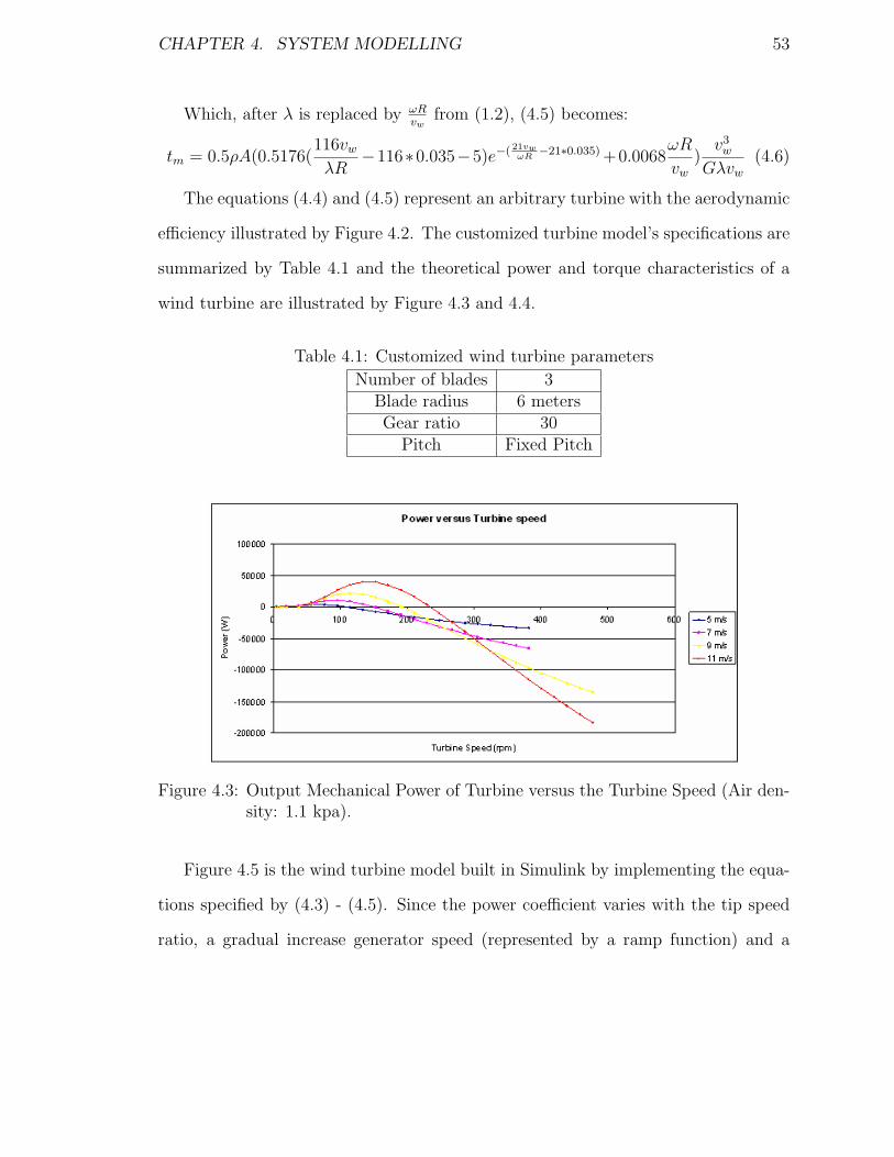
CHAPTER 4. SYSTEM MODELLING 53
Which, after λ is replaced by ωRvw
from (1.2), (4.5) becomes:
tm = 0.5ρA(0.5176(116vw
λR−116∗0.035−5)e−( 21vw
ωR−21∗0.035) +0.0068
ωR
vw
)v3
w
Gλvw
(4.6)
The equations (4.4) and (4.5) represent an arbitrary turbine with the aerodynamic
efficiency illustrated by Figure 4.2. The customized turbine model’s specifications are
summarized by Table 4.1 and the theoretical power and torque characteristics of a
wind turbine are illustrated by Figure 4.3 and 4.4.
Table 4.1: Customized wind turbine parameters
Number of blades 3Blade radius 6 metersGear ratio 30
Pitch Fixed Pitch
Figure 4.3: Output Mechanical Power of Turbine versus the Turbine Speed (Air den-sity: 1.1 kpa).
Figure 4.5 is the wind turbine model built in Simulink by implementing the equa-
tions specified by (4.3) - (4.5). Since the power coefficient varies with the tip speed
ratio, a gradual increase generator speed (represented by a ramp function) and a
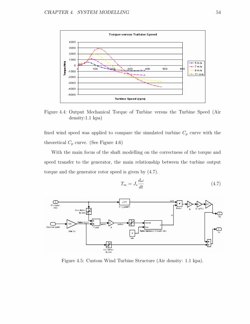
CHAPTER 4. SYSTEM MODELLING 54
Figure 4.4: Output Mechanical Torque of Turbine versus the Turbine Speed (Airdensity:1.1 kpa)
fixed wind speed was applied to compare the simulated turbine Cp curve with the
theoretical Cp curve. (See Figure 4.6)
With the main focus of the shaft modelling on the correctness of the torque and
speed transfer to the generator, the main relationship between the turbine output
torque and the generator rotor speed is given by (4.7).
Tm = Jsdω
dt(4.7)
Figure 4.5: Custom Wind Turbine Structure (Air density: 1.1 kpa).

CHAPTER 4. SYSTEM MODELLING 55
Figure 4.6: Custom Wind Turbine (Air density: 1.1 kpa).
Where Tm is the mechanical torque from the wind turbine, Js is the total system
inertia, and ω is the angular velocity of the turbine shaft. The total system inertia,
Js, is given by:
Js = JT + JG(G) (4.8)
Where JT is the inertia of the turbine, JG is the inertia of the machine, and G is
the gear ratio between the turbine and the generator.
G =ω2
ω1
=N2
N1
(4.9)
Figure 4.8 shows the complete wind turbine model built with PSIM 7.0 simulation
software [8]. In PSIM, there is an analogy between electrical parameters (current, volt-
age, and capacitance) and mechanical parameters (torque, angular rotational speed,
and inertia) that is used to create a custom mechanical load model. To achieve this,
a dependent current source is placed in parallel with a capacitor (See figure 4.7) [8].
Figure 4.7 is an example of a custom mechanical load used with an induction ma-
chine, but it can be used for all machines in the PSIM library. The capacitor voltage
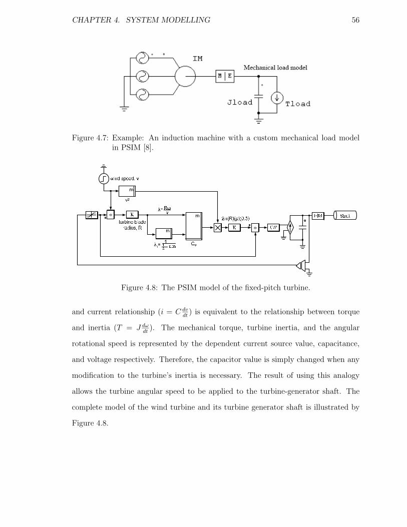
CHAPTER 4. SYSTEM MODELLING 56
Figure 4.7: Example: An induction machine with a custom mechanical load modelin PSIM [8].
Figure 4.8: The PSIM model of the fixed-pitch turbine.
and current relationship (i = C dvdt
) is equivalent to the relationship between torque
and inertia (T = J dωdt
). The mechanical torque, turbine inertia, and the angular
rotational speed is represented by the dependent current source value, capacitance,
and voltage respectively. Therefore, the capacitor value is simply changed when any
modification to the turbine’s inertia is necessary. The result of using this analogy
allows the turbine angular speed to be applied to the turbine-generator shaft. The
complete model of the wind turbine and its turbine generator shaft is illustrated by
Figure 4.8.

CHAPTER 4. SYSTEM MODELLING 57
4.2 Power Electronic Interface Analysis
To extract maximum power from the wind by varying the generator speed, a power
electronics interface between the generator and the DC load side must be used to
provide the system with a control parameter. Ultimately, the generator speed is
controlled by changing the loading of the generator by means of the power electronic
converter. As mentioned earlier in chapter 2, the two most common types of power
electronics rectifiers found in WECS applications is the PWM rectifier and the single
phase boost converter [27]. The advantages of using an PWM rectifier is that it
does not require any inductors or capacitors in the circuit. Also, by applying PWM
techniques to the rectifier, good control flexibility can be obtained. However, since the
PWM rectifier requires six switches in the circuit, the control scheme would be quite
complicated. Since the purpose of this thesis is to evaluate the effectiveness of the
algorithm, a single phase boost converter is used. Compared to the PWM rectifier, the
single phase boost converter requires only one switch in the circuit to be controlled. As
a result, a simple duty ratio control loop can be used to adjust the pulse width of the
switch to control the loading of the generator. Also, by operating the boost converter
in discontinuous conduction mode (DCM), the boost inductor current follows the
envelope of the rectified AC generator voltage and close-to-sinusoidal current can be
obtained at the output of the generator. Operating the boost converter in DCM also
helps to reduce the switching losses of the switch [28].
4.2.1 Design of Boost Converter
Since the main scope of this thesis is to verify the functionality of the proposed
adaptive control algorithm in MPPT applications for WECS, the boost converter

CHAPTER 4. SYSTEM MODELLING 58
is chosen as the front-end power converter connected between the PMSG and DC
load side. The design specifications are listed in Table 4.2. In this design example,
the boost converter was designed for the highest rated wind speed of 9 m/s. The
maximum boost inductor value (Lmax) that can be used to operate the boost converter
in DCM is given by (4.10). Also, to achieve very low ripple output voltage, the
minimum output capacitor value (Cmin) is calculated by (4.11), where ∆V is 0.5% of
the rated output voltage.
Table 4.2: Design specifications for boost converter.
Output Power 20kWLoad resistance (R) 20Ω
switching frequency (fs) 5kHzOutput voltage (Vo) 632V
Lmax =TsVo
2Io
(D)(1 − D)2 (4.10)
Cmin =Vo
∆V
DTs
R(4.11)
For the system used in this thesis, Lmax is calculated to be 470µH from (4.10)
and Cmin is calculated to be 600µF from (4.11). In the actual design, to ensure that
the boost converter always operates in DCM under different wind conditions and that
the output voltage has very low ripple, L is selected to be 200µH and C is 2000µF
respectively.
4.2.2 Overall Control Concept
Figure 4.1 illustrates the overall system diagram where the MPPT block encapsulates
the algorithm and the feedback control block. The system in this study uses a speed

CHAPTER 4. SYSTEM MODELLING 59
loop control concept where the generator speed is directly compared to the reference
speed generated by the MPPT block. The concept used in this thesis is based on the
concept discussed in [19]. The MPPT block uses the rotor speed and the output power
of the boost converter (by using the DC voltage and output current) to determine
a proper speed reference. The speed error signal is obtained from comparing the
reference speed and the rotor speed and is fed into the compensator. The compensator
output signal is the duty ratio (d) for the boost converter. By changing d, the output
power of the boost converter (and thus the generator loading) is changed.
4.2.3 Feedback Loop Analysis
The block diagram of the closed loop system is shown in Figure 4.9, where ∧ represents
a small signal quantity. To design a proper compensator so that all the stability
requirements are met and enable the MPPT control block to accurately determine
the optimum output power point for a particular wind speed, small-signal modeling
of the boost converter is performed. The compensator is then designed using the
SISO toolbox from MATLAB. All the relevant information including the the final
closed-loop system Bode plot will be given in this section to verify all the theoretical
analysis.
A. Modeling of DCM Boost Converter
Modeling of boost converter has been done extensively in literature [29][30]. The
small signal model of the DCM boost converter in this design example is obtained
based on the average circuit model proposed by Erickson [31]. Figure 4.10 and figure
4.11 show the corresponding average circuit model and small signal model of the boost
converter respectively, where i1, i2 , i3 and i4 are given in (4.12), (4.13), (4.14) and
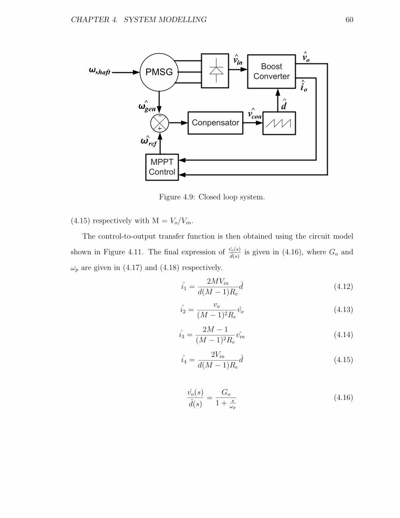
CHAPTER 4. SYSTEM MODELLING 60og e nr e f
i n+ _ c o n
s h a f t o^ ^ ^^^^ ^
Figure 4.9: Closed loop system.
(4.15) respectively with M = Vo/Vin.
The control-to-output transfer function is then obtained using the circuit model
shown in Figure 4.11. The final expression of vo(s)
d(s)is given in (4.16), where Go and
ωp are given in (4.17) and (4.18) respectively.
i1 =2MVin
d(M − 1)Re
d (4.12)
i2 =vo
(M − 1)2Re
vo (4.13)
i3 =2M − 1
(M − 1)2Re
vin (4.14)
i4 =2Vin
d(M − 1)Re
d (4.15)
vo(s)
d(s)=
Go
1 + sωp
(4.16)
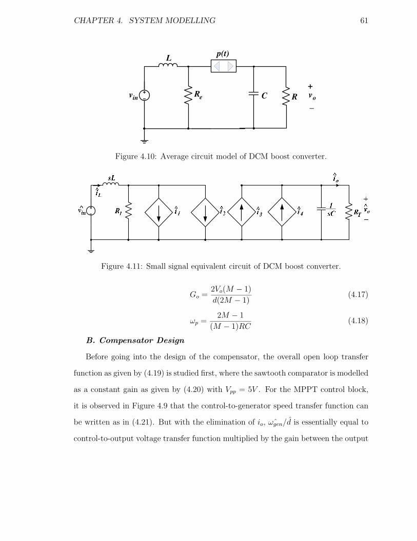
CHAPTER 4. SYSTEM MODELLING 61
C
L
inv RRe
p(t)
ov+
_
Figure 4.10: Average circuit model of DCM boost converter.
Figure 4.11: Small signal equivalent circuit of DCM boost converter.
Go =2Vo(M − 1)
d(2M − 1)(4.17)
ωp =2M − 1
(M − 1)RC(4.18)
B. Compensator Design
Before going into the design of the compensator, the overall open loop transfer
function as given by (4.19) is studied first, where the sawtooth comparator is modelled
as a constant gain as given by (4.20) with Vpp = 5V . For the MPPT control block,
it is observed in Figure 4.9 that the control-to-generator speed transfer function can
be written as in (4.21). But with the elimination of io, ˆωgen/d is essentially equal to
control-to-output voltage transfer function multiplied by the gain between the output

CHAPTER 4. SYSTEM MODELLING 62
voltage (vo) and the generator speed (ωgen) as shown in (4.21). Figure 4.12 illustrates
the relationship between ωgen and the output voltage found through system testing.
The corresponding relationship is given in (4.22). It is observed that the DC output
voltage (vo) and the generator speed (ωgen) presents a fairly linear relationship. In
this design, a gain of 5 is obtained. The overall open-loop transfer function is then
given in (4.23). It exhibits a single pole characteristic that is contributed by the DC-
link capacitor. It this case, the single pole occurs at ω = 111.82rad/s as calculated
from (4.16).
Topen(s) = Tcomp(s)Tboost(s)Tω/v(s) (4.19)
Tcomp(s) =1
Vpp
=1
5(4.20)
ˆωgen
d=
(
ˆωgen
voio
)(
voio
d
)
=ˆωgen
vo
vo
d(4.21)
Tω/v(s) =ωgen
vo
(4.22)
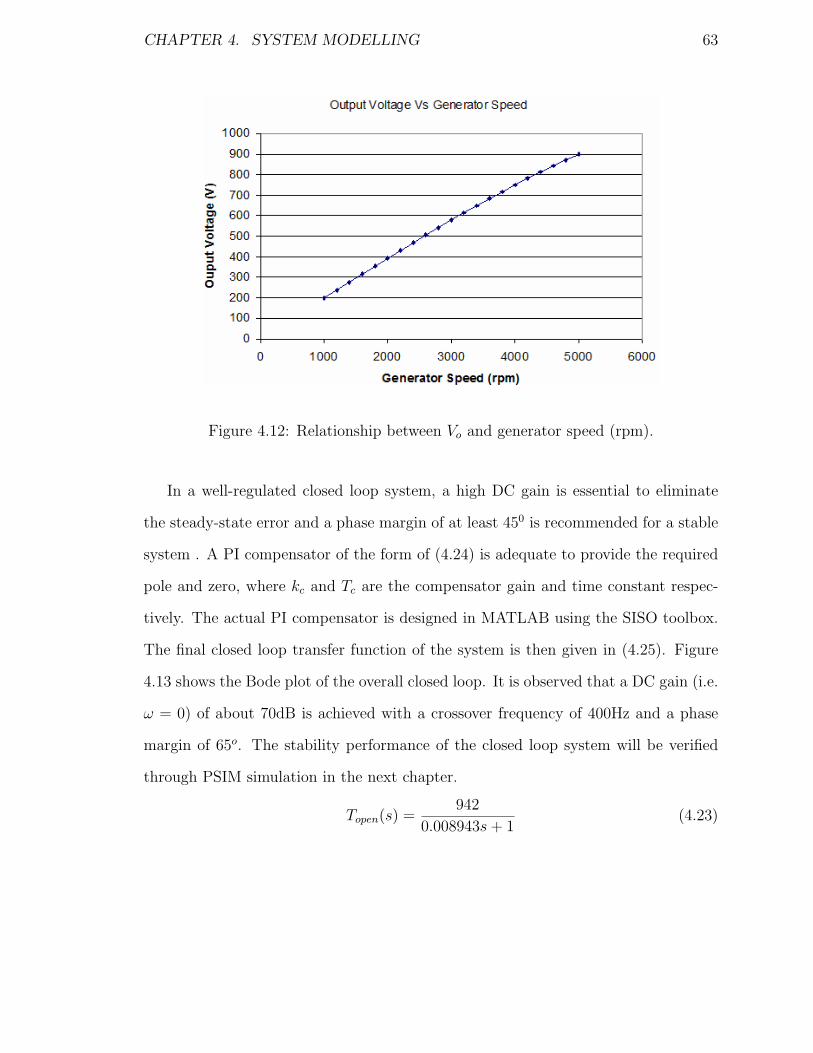
CHAPTER 4. SYSTEM MODELLING 63
Figure 4.12: Relationship between Vo and generator speed (rpm).
In a well-regulated closed loop system, a high DC gain is essential to eliminate
the steady-state error and a phase margin of at least 450 is recommended for a stable
system . A PI compensator of the form of (4.24) is adequate to provide the required
pole and zero, where kc and Tc are the compensator gain and time constant respec-
tively. The actual PI compensator is designed in MATLAB using the SISO toolbox.
The final closed loop transfer function of the system is then given in (4.25). Figure
4.13 shows the Bode plot of the overall closed loop. It is observed that a DC gain (i.e.
ω = 0) of about 70dB is achieved with a crossover frequency of 400Hz and a phase
margin of 65o. The stability performance of the closed loop system will be verified
through PSIM simulation in the next chapter.
Topen(s) =942
0.008943s + 1(4.23)
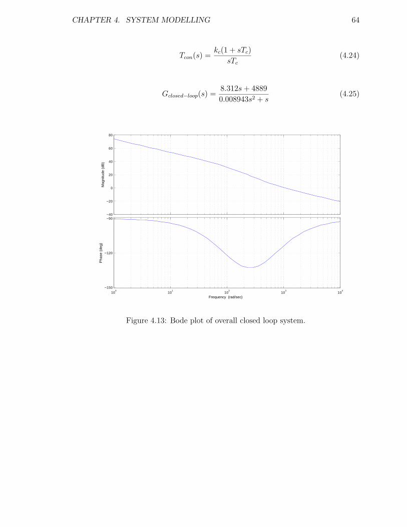
CHAPTER 4. SYSTEM MODELLING 64
Tcon(s) =kc(1 + sTc)
sTc
(4.24)
Gclosed−loop(s) =8.312s + 4889
0.008943s2 + s(4.25)
−40
−20
0
20
40
60
80
Mag
nitu
de (
dB)
100
101
102
103
104
−150
−120
−90
Pha
se (
deg)
Frequency (rad/sec)
Figure 4.13: Bode plot of overall closed loop system.

Chapter 5
Algorithm Performance
5.1 Simulation Model Overview
The complete wind energy conversion system was built in PSIM 7.0, and is as illus-
trated in Figure 5.1. The detailed diagram of the wind turbine and turbine shaft
in Figure 5.1 is given by Fig. 4.7. The C++ programmable script block is used to
implement the maximum power point tracking algorithm. The algorithm requires
the wind speed, generator speed, output voltage and output current as an input.
Since the algorithm requires an anemometer to monitor the wind speed and calculate
the turbine’s internal TSR, the wind speed is directly fed into the algorithm in the
simulation. The generator speed input allows the algorithm to determine whether
the generator speed has reached the reference speed as desired. The output voltage
and current together provides the algorithm with knowledge of the output power.
Information regarding the output power, generator speed, and wind speed allow the
algorithm to determine the system’s maximum power points.
65
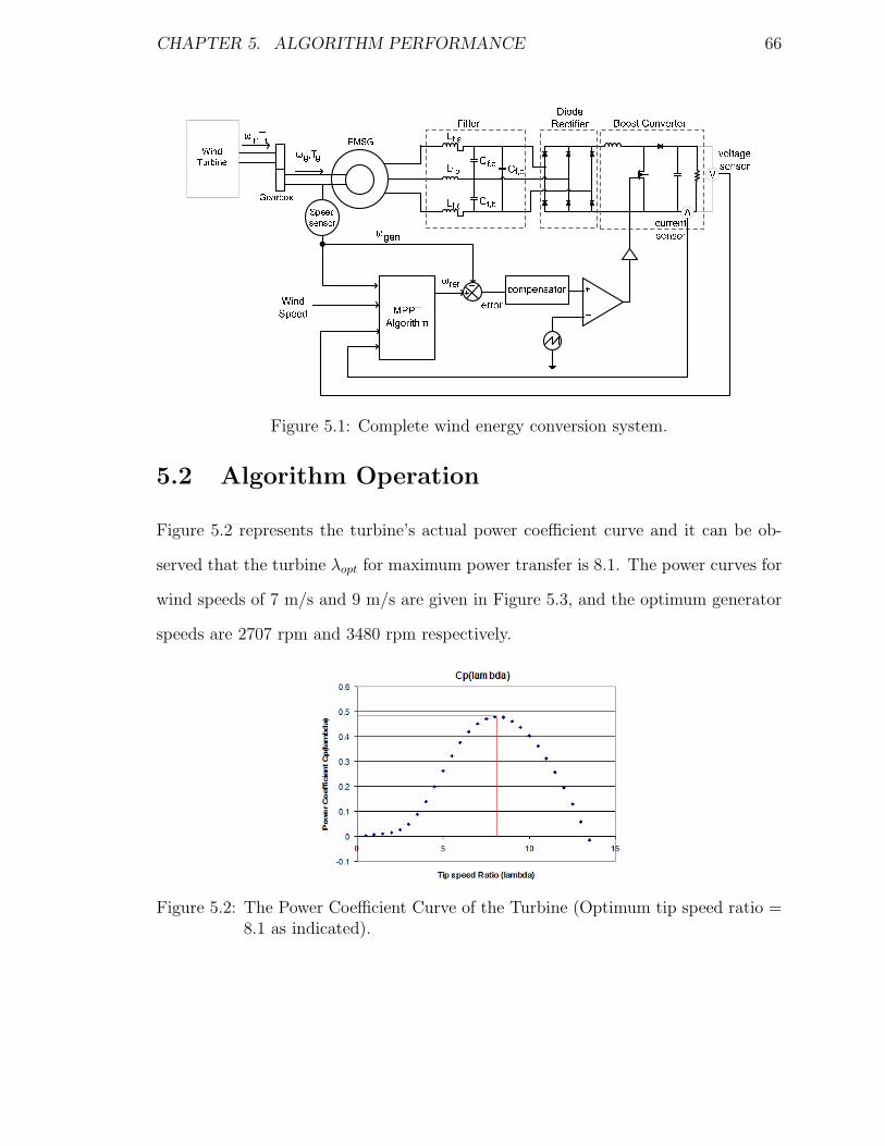
CHAPTER 5. ALGORITHM PERFORMANCE 66
Figure 5.1: Complete wind energy conversion system.
5.2 Algorithm Operation
Figure 5.2 represents the turbine’s actual power coefficient curve and it can be ob-
served that the turbine λopt for maximum power transfer is 8.1. The power curves for
wind speeds of 7 m/s and 9 m/s are given in Figure 5.3, and the optimum generator
speeds are 2707 rpm and 3480 rpm respectively.
Figure 5.2: The Power Coefficient Curve of the Turbine (Optimum tip speed ratio =8.1 as indicated).
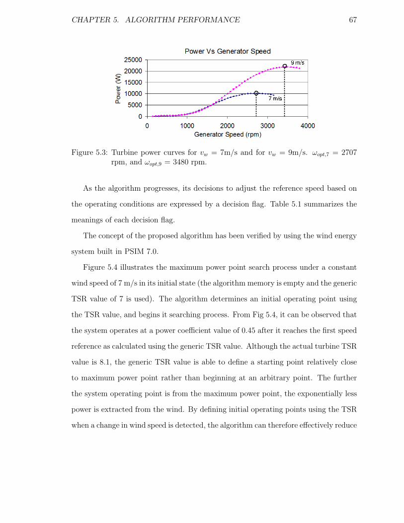
CHAPTER 5. ALGORITHM PERFORMANCE 67
Figure 5.3: Turbine power curves for vw = 7m/s and for vw = 9m/s. ωopt,7 = 2707rpm, and ωopt,9 = 3480 rpm.
As the algorithm progresses, its decisions to adjust the reference speed based on
the operating conditions are expressed by a decision flag. Table 5.1 summarizes the
meanings of each decision flag.
The concept of the proposed algorithm has been verified by using the wind energy
system built in PSIM 7.0.
Figure 5.4 illustrates the maximum power point search process under a constant
wind speed of 7 m/s in its initial state (the algorithm memory is empty and the generic
TSR value of 7 is used). The algorithm determines an initial operating point using
the TSR value, and begins it searching process. From Fig 5.4, it can be observed that
the system operates at a power coefficient value of 0.45 after it reaches the first speed
reference as calculated using the generic TSR value. Although the actual turbine TSR
value is 8.1, the generic TSR value is able to define a starting point relatively close
to maximum power point rather than beginning at an arbitrary point. The further
the system operating point is from the maximum power point, the exponentially less
power is extracted from the wind. By defining initial operating points using the TSR
when a change in wind speed is detected, the algorithm can therefore effectively reduce
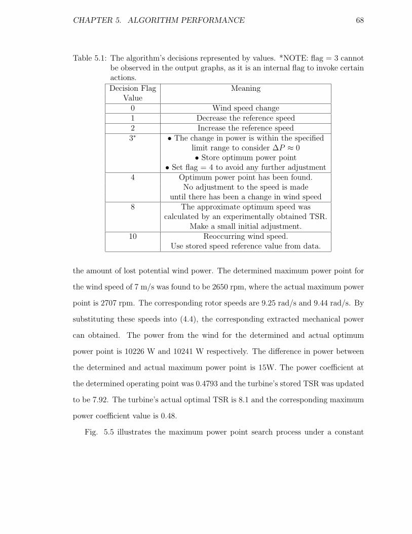
CHAPTER 5. ALGORITHM PERFORMANCE 68
Table 5.1: The algorithm’s decisions represented by values. *NOTE: flag = 3 cannotbe observed in the output graphs, as it is an internal flag to invoke certainactions.
Decision Flag MeaningValue
0 Wind speed change1 Decrease the reference speed2 Increase the reference speed3∗ • The change in power is within the specified
limit range to consider ∆P ≈ 0• Store optimum power point
• Set flag = 4 to avoid any further adjustment4 Optimum power point has been found.
No adjustment to the speed is madeuntil there has been a change in wind speed
8 The approximate optimum speed wascalculated by an experimentally obtained TSR.
Make a small initial adjustment.10 Reoccurring wind speed.
Use stored speed reference value from data.
the amount of lost potential wind power. The determined maximum power point for
the wind speed of 7 m/s was found to be 2650 rpm, where the actual maximum power
point is 2707 rpm. The corresponding rotor speeds are 9.25 rad/s and 9.44 rad/s. By
substituting these speeds into (4.4), the corresponding extracted mechanical power
can obtained. The power from the wind for the determined and actual optimum
power point is 10226 W and 10241 W respectively. The difference in power between
the determined and actual maximum power point is 15W. The power coefficient at
the determined operating point was 0.4793 and the turbine’s stored TSR was updated
to be 7.92. The turbine’s actual optimal TSR is 8.1 and the corresponding maximum
power coefficient value is 0.48.
Fig. 5.5 illustrates the maximum power point search process under a constant
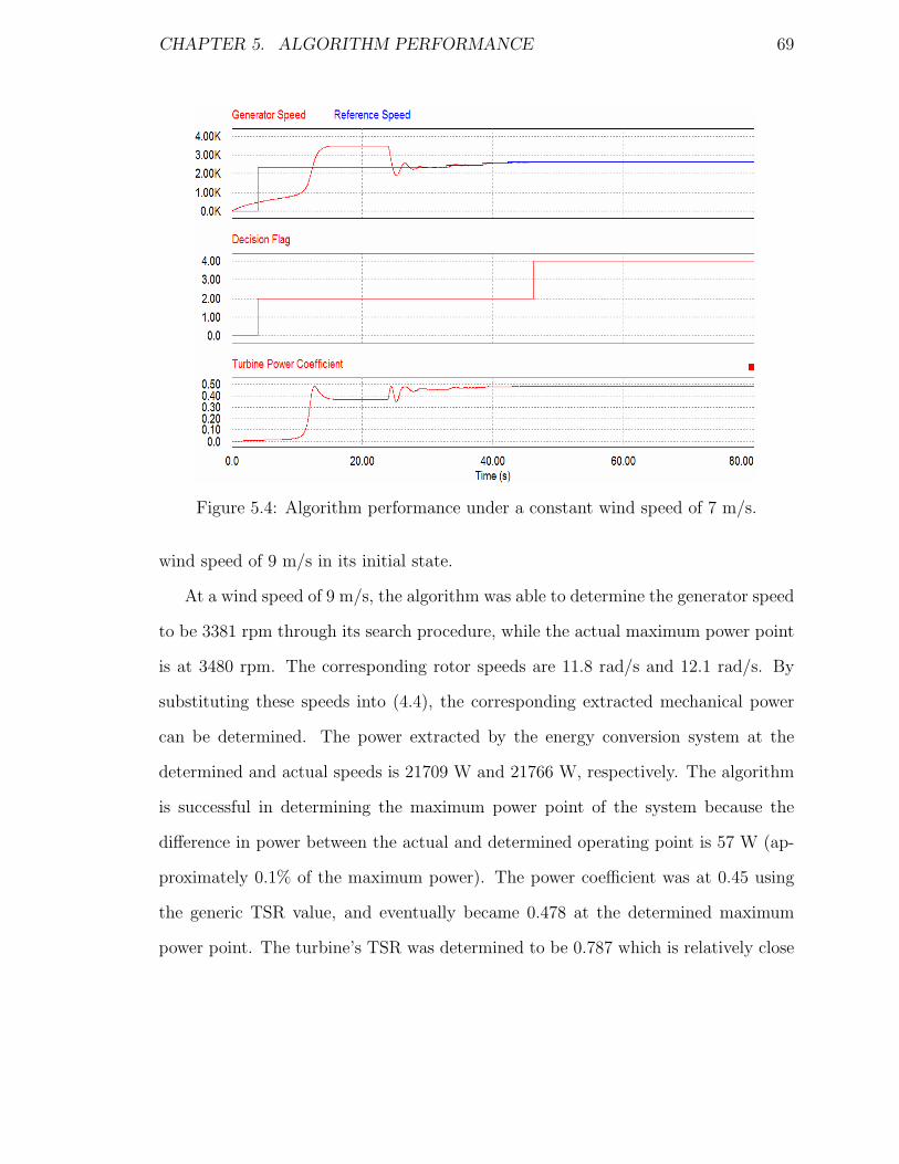
CHAPTER 5. ALGORITHM PERFORMANCE 69
Figure 5.4: Algorithm performance under a constant wind speed of 7 m/s.
wind speed of 9 m/s in its initial state.
At a wind speed of 9 m/s, the algorithm was able to determine the generator speed
to be 3381 rpm through its search procedure, while the actual maximum power point
is at 3480 rpm. The corresponding rotor speeds are 11.8 rad/s and 12.1 rad/s. By
substituting these speeds into (4.4), the corresponding extracted mechanical power
can be determined. The power extracted by the energy conversion system at the
determined and actual speeds is 21709 W and 21766 W, respectively. The algorithm
is successful in determining the maximum power point of the system because the
difference in power between the actual and determined operating point is 57 W (ap-
proximately 0.1% of the maximum power). The power coefficient was at 0.45 using
the generic TSR value, and eventually became 0.478 at the determined maximum
power point. The turbine’s TSR was determined to be 0.787 which is relatively close
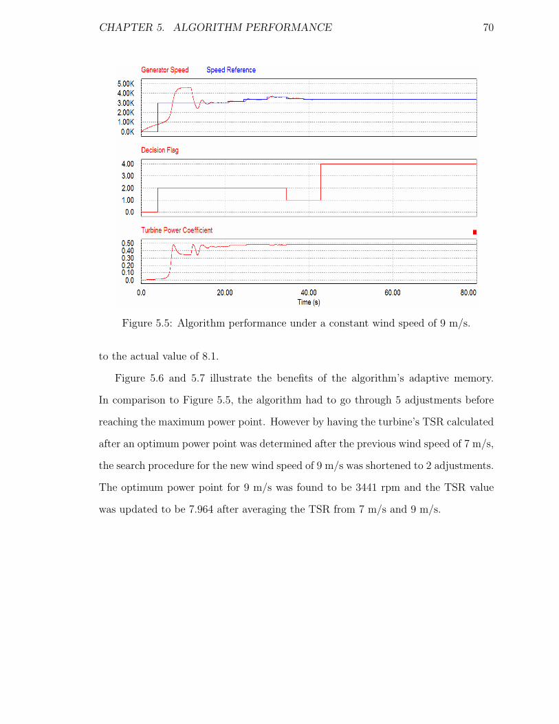
CHAPTER 5. ALGORITHM PERFORMANCE 70
Figure 5.5: Algorithm performance under a constant wind speed of 9 m/s.
to the actual value of 8.1.
Figure 5.6 and 5.7 illustrate the benefits of the algorithm’s adaptive memory.
In comparison to Figure 5.5, the algorithm had to go through 5 adjustments before
reaching the maximum power point. However by having the turbine’s TSR calculated
after an optimum power point was determined after the previous wind speed of 7 m/s,
the search procedure for the new wind speed of 9 m/s was shortened to 2 adjustments.
The optimum power point for 9 m/s was found to be 3441 rpm and the TSR value
was updated to be 7.964 after averaging the TSR from 7 m/s and 9 m/s.
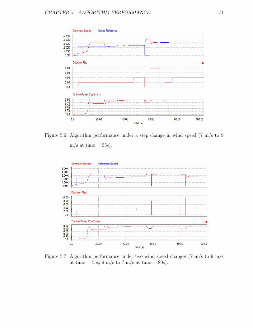
CHAPTER 5. ALGORITHM PERFORMANCE 71
Figure 5.6: Algorithm performance under a step change in wind speed (7 m/s to 9
m/s at time = 55s).
Figure 5.7: Algorithm performance under two wind speed changes (7 m/s to 9 m/sat time = 55s, 9 m/s to 7 m/s at time = 80s).
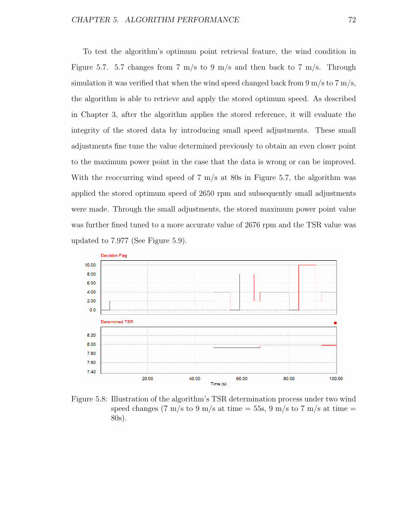
CHAPTER 5. ALGORITHM PERFORMANCE 72
To test the algorithm’s optimum point retrieval feature, the wind condition in
Figure 5.7. 5.7 changes from 7 m/s to 9 m/s and then back to 7 m/s. Through
simulation it was verified that when the wind speed changed back from 9 m/s to 7 m/s,
the algorithm is able to retrieve and apply the stored optimum speed. As described
in Chapter 3, after the algorithm applies the stored reference, it will evaluate the
integrity of the stored data by introducing small speed adjustments. These small
adjustments fine tune the value determined previously to obtain an even closer point
to the maximum power point in the case that the data is wrong or can be improved.
With the reoccurring wind speed of 7 m/s at 80s in Figure 5.7, the algorithm was
applied the stored optimum speed of 2650 rpm and subsequently small adjustments
were made. Through the small adjustments, the stored maximum power point value
was further fined tuned to a more accurate value of 2676 rpm and the TSR value was
updated to 7.977 (See Figure 5.9).
Figure 5.8: Illustration of the algorithm’s TSR determination process under two windspeed changes (7 m/s to 9 m/s at time = 55s, 9 m/s to 7 m/s at time =80s).
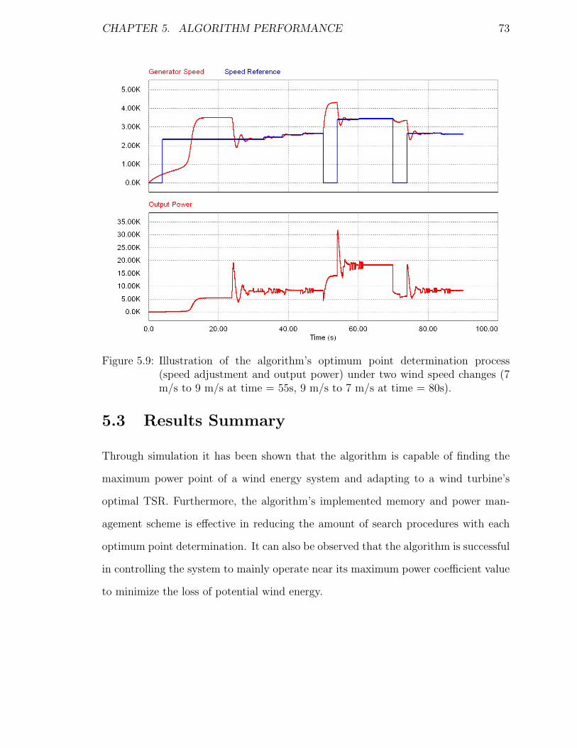
CHAPTER 5. ALGORITHM PERFORMANCE 73
Figure 5.9: Illustration of the algorithm’s optimum point determination process(speed adjustment and output power) under two wind speed changes (7m/s to 9 m/s at time = 55s, 9 m/s to 7 m/s at time = 80s).
5.3 Results Summary
Through simulation it has been shown that the algorithm is capable of finding the
maximum power point of a wind energy system and adapting to a wind turbine’s
optimal TSR. Furthermore, the algorithm’s implemented memory and power man-
agement scheme is effective in reducing the amount of search procedures with each
optimum point determination. It can also be observed that the algorithm is successful
in controlling the system to mainly operate near its maximum power coefficient value
to minimize the loss of potential wind energy.

Chapter 6
Summary and Conclusions
6.1 Summary
With rising concerns over rising energy prices, depletion of natural resources and
pollution, environmentally friendly energy resources like wind energy are becoming
more prominent. Wind energy is inexhaustible, safe, has no harmful by products and
is capable of supplying substantial amounts of power. The unpredictable availability
of wind however, only allows it to become a secondary source of power. In order
to harness as much power from the wind as possible while it is available, intelligent
control strategies must be implemented. With technological advancements in wind
turbine aerodynamics and power electronic interfaces, wind energy can be considered
to be an excellent renewable supplementary energy source. Power electronic interfaces
and intelligent control strategies make wind energy viable and attractive despite its
intermittent availability.
This thesis provides extensive background knowledge on the wind energy market,
turbine technology, and energy conversion. The main purpose of this thesis is to
74

CHAPTER 6. SUMMARY AND CONCLUSIONS 75
design and develop an algorithm to enable maximum power transfer under fluctuating
wind conditions. Various algorithms and control schemes that attempt to extract the
maximum power from the wind were studied and presented. The concepts were
grouped into three main categories: i) customized, ii) continual adjustments, iii)
adaptive. The study identified the main problems in existing maximum power point
extraction algorithms, and then used them as guidelines for the algorithm design.
The main problems are customization, speed, and wasted power. The customization
problem refers to the preprogramming of a turbine’s characteristic into an algorithm,
making it effective only for the turbine it was originally designed for. The decisions
and structure of each customized algorithm is based on the turbine characteristics and
each wind turbine has its distinct characteristic. Therefore, customized algorithms
cannot be easily reused onto other turbines and it would be costly to continually
design a new algorithm. The speed of the algorithm has a great effect on the amount
of wasted potential wind power. A wind turbine does not naturally operate at its
most efficient operating point, and due to the shape of wind turbine power curves,
a significant amount of wind power can be left unharnessed. As a solution to these
problems, the proposed algorithm uses a modified version of an established concept
known as the hill climb search (HCS) algorithm. The modified concept uses the
standard concept in conjunction with intelligent memory and power management
schemes to enable the algorithm to quickly determine maximum power points and
adapt to any given turbine.
Since literature did not provide methods for the design of a complete wind energy
conversion system, the system used in this thesis was built to resemble those in liter-
ature. A wind energy conversion system with a custom wind turbine was constructed

CHAPTER 6. SUMMARY AND CONCLUSIONS 76
based on the wind turbine model in MATLAB Simulink. The generator was directly
incorporated into the system by using the model provided by PSIM, and the PMSG
parameters were based on literature values. In order to build the system for easy
algorithm verification, the boost converter configuration was used. The boost con-
verter configuration is a common method used in variable speed PMSG wind turbine
applications [6][8][19]. To ensure that the system exhibited characteristics that were
similar to the wind energy system found in literature, extensive tests were performed.
6.2 Contributions
The main contributions of this thesis are summarized as follows:
1. The proposed algorithm structure incorporates intelligent memory to achieve
unsupervised training. Because the optimal TSR that corresponds to a maxi-
mum power coefficient for all wind speeds, the unsupervised training is achieved
by using the maximum power point search data to determine an experimentally
TSR value.
2. The algorithm is easily configured for any given wind turbine because it does
not require previous knowledge or the turbine characteristics or the wind en-
ergy conversion system configuration to make its decisions. The algorithm is
structured so that the internal turbine characteristics are determined through
operation. Although a TSR value is used in the initial stage of the algorithm,
it is a generic optimum TSR for a horizontal-axis, three-blade wind turbine
3. Maximum power can be quickly extracted under wind fluctuations due to the
use of the TSR relationship. By using the TSR relationship, the algorithm can

CHAPTER 6. SUMMARY AND CONCLUSIONS 77
immediately jump to an operating point very close to the maximum power point
rather than operating an arbitrary point depending on the systems operating
conditions. With the added memory in the system, the algorithm is also capable
of jumping to the maximum power point in the case of a reoccurring wind speed.
This allows the system to bypass any redundant search procedures and therefore
minimizes the loss in potential power.
4. A complete wind energy system has been designed in this thesis. The modeling
of the wind turbine to the DC-DC converter for a front-end rectifier wind energy
system is provided.
6.3 Future Works
Future works related to the proposed circuit could be summarized as follows:
1. Experimental verification of the proposed algorithm by using a low power wind
turbine. The proposed algorithm can be implemented by using field programmable
gate array (FPGA) techniques or digital signal processors (DSP).
2. A new algorithm that can provide comparable performance without the use of
an anemometer, can be developed. Sensorless wind energy systems are more
cost effective and robust.
3. Different converter topologies can be implemented to provide better control.
Such as matrix converters and PWM rectifiers.
4. In this thesis, the proposed algorithm is tested under step changes in wind. To
obtain more practical performance results to further improve on the design, a

CHAPTER 6. SUMMARY AND CONCLUSIONS 78
wind prediction scheme can be developed to model realistic wind behavior.
6.4 Conclusion
Due to wind’s unpredictable nature, power management concepts are necessary to
extract as much power as possible from the wind when it becomes available. The
proposed algorithm has been developed to maintain the system at its highest possible
efficiency by using its memory feature to infer the optimum rotor speeds for wind
speeds that have not occurred before. Another feature of the proposed algorithm
is that it can be easily customized for various wind turbines since it is independent
of turbine characteristics. The proposed algorithm uses a modified version of HCS
and intelligent memory to implement its power management scheme. This algorithm
is most suitable for smaller grid or battery connected wind energy systems. PSIM
simulation studies have confirmed the effectiveness of the proposed algorithm.

Bibliography
[1] “Global wind 2007 report,” May 2008.
[2] “Global wind 2006 report,” June 2007.
[3] M. Idan, D. Lior, and G. Shaviv, “A robust controller for a novel variable
speed wind turbine transmission,” Journal of Solar Energy Engineering, vol. 120,
pp. 247–252, 1998.
[4] R. Gilbert, “Regulatory choices: A perspective on developments in energy pol-
icy,” Mathematical and Computational Applications, pp. 10–17, December 2007.
[5] S. Muller, M. Deicke, and R.-W. De Docker, “Adjustable speed generators for
wind turbines based on doubly-fed induction machines and 4-quadrant igbt con-
verters linked to the rotor,” IEEE Industry Applications Conference, vol. 4,
pp. 2254–2259, October 2000.
[6] J. Marques, H. Pinheiro, H. Grundling, J. Pinheiro, and H. Hey, “A survey
on variable-speed wind turbine system,” Proceedings of Brazilian conference of
electronics of power, vol. 1, pp. 732 – 738, 2003.
79

BIBLIOGRAPHY 80
[7] Q. Wang and L.-C. Chang, “An intelligent maximum power extraction algorithm
for inverter-based variable speed wind turbine systems,” IEEE Transactions on
Power Electronics, vol. 19, pp. 1242–1249, September 2004.
[8] P. Inc, PSIM: User Manual. Powersim Inc., 1 ed., 2001.
[9] T. I. of Electrical and E. E. Inc, “Ieee canadian review: Green power,” Mathe-
matical and Computational Applications, pp. 10–17, December 2007.
[10] C. W. E. Association, “Wind facts - an introduction to wind power,” Mathemat-
ical and Computational Applications, 2007.
[11] F.-S. dos Reis, K. Tan, and S. Islam, “Using pfc for harmonic mitigation in
wind turbine energy conversion systems,” IEEE Industrial Electronics Society
Conference, pp. 3100–3105, November 2004.
[12] “windpower.org,” 2006.
[13] G. Moor and H. Beukes, “Power point trackers for wind turbines,” Power Elec-
tronics Specialist Conference (PESC), pp. 2044–2049, 2004.
[14] Y. Song, B. Dhinakaran, and X. Bao, “Variable speed control of wind turbines
using nonlinear and adaptive algorithms,” Journal of Wind Engineering and
Industrial Aerodynamics., vol. 85, no. 3, pp. 293–308, 2000.
[15] D.-S. Zinger and E. Muljadi, “Annualized wind energy improvement using vari-
able speeds,” IEEE Transactions on Industry Applications, vol. 33, pp. 1444–
1447, November 1997.
BIBLIOGRAPHY 81
[16] M. Chinchilla, S. Arnaltes, and J.-C. Burgos, “Control of permanent-magnet
generators applied to variable-speed wind-energy systems connected to the grid,”
IEEE Transactions on Energy Conversion, vol. 21, pp. 130–135, March 2006.
[17] E. Koutroulis and K. Kalaitzakis, “Design of a maximum power tracking sys-
tem for wind-energy-conversion applications,” IEEE Transactions on Industrial
Electronics, vol. 53, April 2006.
[18] T.-S. Shikha, Bhatti, and D.-P. Kothari, “A new vertical axis wind rotor using
convergent nozzles,” Large Engineering Systems Conference on Power Engineer-
ing, pp. 177–181, May 2003.
[19] I. Munteanu, A. I. Bratcu, N. Cutululis, and E. Ceanga, Optimal Control of Wind
Energy Systems: Towards a Global Approach. Springer-Verlag London Limited,
1 ed., 2008.
[20] F. Blaabjerg and Z. Chen, Power Electronics for Modern Wind Turbines. Morgan
& Claypool Publishers, 1 ed., 2006.
[21] S. Bhowmik, R. Spee, and J.-H.-R. Enslin, “Performance optimization for doubly
fed wind power generation systems,” IEEE Transactions on Industry Applica-
tions, vol. 35, pp. 949–958, July/August 1999.
[22] R. Datta and V.-T. Ranganathan, “A method of tracking the peak power points
for a variable speed wind energy conversion system,” IEEE Transactions on
Energy Conversion, vol. 18, pp. 163–168, March 2003.

BIBLIOGRAPHY 82
[23] T. Nakamura, S. Morimoto, M. Sanada, and Y. Takeda, “Optimum control of
ipmsg for wind generation system,” Power Conversion Conference (PCC), vol. 3,
pp. 1435–1440, 2002.
[24] N.-S. Cetin, M.-A. Yurdusev, R. Ata, and A. Ozdemir, “Assessment of optimum
tip speed ratio of wind turbines,” Mathematical and Computational Applications,
vol. 10, pp. 147–154, March 2005.
[25] A.-B. Raju, K. Chatterjee, and B.-G. Fernandes, “A simple maximum power
point tracker for grid connected variable speed wind energy conversion system
with reduced switch count power converters,” IEEE Power Electronics Specialist
Conference, PESC ’03, pp. 748 – 753, June 2003.
[26] “Wind turbine model,” 2006.
[27] C. Silva, R. Bascope, and D. Oliveira, “Three-phase power factor correction
rectifier applied to wind energy conversion systems,” Applied Power Electronics
Conference and Exposition, 2008. APEC 2008., pp. 768 – 773, Feb 2008.
[28] K.-H. Liu and Y.-L. Lin, “Current waveform distortion in power factor correc-
tion circuits employing discontinuous-mode boost converters,” Power Electronics
Specialists Conference, pp. 825 – 829, June 1989.
[29] Y.-F. Liu and P.-C. Sen, “A general unified large signal model for current pro-
grammed dc-to-dc converters,” IEEE Transactions on Power Electronics, pp. 414
– 424, July 1994.

BIBLIOGRAPHY 83
[30] J. Sun, D. Mitchell, M. Greuel, P. Krein, and R. Bass, “Modeling of pwm con-
verters in discontinuous conduction mode. a reexamination,” Power Electronics
Specialists Conference, 1998. PESC 98, pp. 615 – 622, May 1998.
[31] E. Rogers, “Application note: Understanding boost power stages in switch mode
power supplies,” Texas Instruments, pp. 1–32, March 1999.