An Adaptive Finite Element Eigenvalue Solver of …gedicke/preprints/CG_2012.pdf · AN ADAPTIVE FINITE ELEMENT EIGENVALUE SOLVER OF ... lustrates the asymptotic quasi-optimal computational

AN ADAPTIVE FINITE ELEMENT EIGENVALUESOLVER OF ASYMPTOTIC QUASI-OPTIMAL

COMPUTATIONAL COMPLEXITY?

CARSTEN CARSTENSEN AND JOSCHA GEDICKE

Abstract. This paper presents a combined adaptive finite ele-ment method with an iterative algebraic eigenvalue solver for asymmetric eigenvalue problem of asymptotic quasi-optimal compu-tational complexity. The analysis is based on a direct approach foreigenvalue problems and allows the use of higher-order conformingfinite element spaces with fixed polynomial degree. The asymptoticquasi-optimal adaptive finite element eigenvalue solver (AFEMES)involves a proper termination criterion for the algebraic eigenvaluesolver and does not need any coarsening. Numerical evidence il-lustrates the asymptotic quasi-optimal computational complexityin 2 and 3 dimensions.

1. Introduction

The eigenvalue problems for symmetric second-order elliptic bound-ary value problems can be discretised with some adaptive finite el-ement method (AFEM). In practice, the resulting finite-dimensionalgeneralised eigenvalue problems are solved iteratively. Thus, the com-putation involves the discretisation error of some AFEM as well as theerror left from the termination of some iterative algebraic eigenvaluesolver. This paper presents the first adaptive finite element eigenvaluesolver (AFEMES) of overall asymptotic quasi-optimal complexity, i.e.,for sufficiently small mesh-sizes the error is optimal up to a genericmultiplicative constant. AFEMES is shown in the pseudocode below.

The algorithm computes one fixed simple eigenvalue. The adaptivemesh refinement via subroutines Mark and Refine is well established inthe finite element community [BDD04, CKNS08, Dor96, Ste07] whileLAES represents any state-of-the-art iterative eigenvalue solver well est-

2000 Mathematics Subject Classification. 65N15, 65N25, 65N30.Key words and phrases. eigenvalue, adaptive finite element method, conver-

gence rates, complexity .? Supported by the DFG Research Center MATHEON “Mathematics for key

technologies”, the World Class University (WCU) program through the NationalResearch Foundation of Korea (NRF) funded by the Ministry of Education, Scienceand Technology R31-2008-000-10049-0, and the graduate school “Berlin Mathemat-ical School” (BMS).

Final version published in SIAM J. Numer. Anal. 50 (2012), no. 3, 1029–1057,http://dx.doi.org/10.1137/090769430.

http://dx.doi.org/10.1137/090769430

2 C. CARSTENSEN AND J. GEDICKE

AFEMESInput: Coarse triangulation T0, initial guess (λ0, u0),

parameters 0 < θ ≤ 1, 0 < ω.

δ0 := 2√ωη0(λ0, u0);

for ` = 0, 1, . . . (until termination)

while ( δ` >√ωη`(λ`, u`) )

δ` := δ`/2; [λ`, u`] := LAES(T`, λ`, u`, δ`); end

T`+1 := Refine(T`,Mark(T`, θ, η`(λ`, u`)));δ`+1 := 2

√ωη`(λ`, u`); λ`+1 := λ`; u`+1 := P `+1

` u`; end

Output: Sequence of triangulations T` and

approximations (λ`, u`).

ablished in the numerical linear algebra community that satisfies theconvergence and complexity assumptions of Section 2. The parame-ters θ and ω depend on the regularity of the solution and η` denotesthe error estimator from Section 4. The prolongation operator fromtriangulation T` onto T`+1 is denoted by P `+1

` . The pseudocode givesone possible error balance of the two error sources of asymptotic quasi-optimal complexity.

The works on asymptotic convergence [CG11, GMZ09, GG09, Sau10]as well as on asymptotic quasi-optimal convergence [DXZ08, GM11]of adaptive mesh refinement for the eigenvalue problem do assumeunrealistically the exact knowledge of algebraic eigenpairs. Anotheroptimality result for linear symmetric operator eigenvalue problems[DRSZ08] is based on coarsening. Assuming a saturation assumption,[MM11, Ney02] present combined adaptive finite element and linearalgebra algorithms.

As a simple model problem for a symmetric, elliptic eigenvalue prob-lem consider the following eigenvalue problem of the Laplace operator:Seek a nontrivial eigenpair (λ, u) ∈ R×H1

0 (Ω;R)∩H2loc(Ω;R) such that

−∆u = λu in Ω and u = 0 on ∂Ω(1.1)

in a bounded Lipschitz domain Ω ⊂ Rn, n = 2, 3. It is well known,that problem (1.1) has countable infinite many solutions with positiveeigenvalues that can be ordered increasingly. For simplicity, this paperis restricted to the case that the eigenvalue of interest λ is a simpleeigenvalue; hence its algebraic and geometric multiplicity equals one.Throughout this paper, standard notations on Sobolev and Lebesguespaces are used.

The weak problem seeks for a nontrivial eigenpair (λ, u) ∈ R×V :=R×H1

0 (Ω;R) with b(u, u) = 1 and

a(u, v) = λb(u, v) for all v ∈ V.

AN AFEMES OF ASYMPTOTIC QUASI-OPTIMAL COMPLEXITY 3

The bilinear forms a(·, ·) and b(·, ·) are defined by

a(u, v) :=

∫Ω

∇u · ∇v dx and b(u, v) :=

∫Ω

uv dx

and induce the norms |||.||| := |.|H1(Ω) on V and ‖.‖ := ‖.‖L2(Ω) on L2(Ω).The conforming finite element space of order k ∈ N for the triangu-

lation T` is defined by

Pk(T`) :=v ∈ H1(Ω) : ∀T ∈ T`, v|T is polynomial of degree ≤ k

.

Let V` := Pk(T`) ∩ V denote the finite-dimensional subspace of fixedorder k > 0 and N` := dim(V`). The corresponding discrete eigen-value problem reads: Seek a nontrivial eigenpair (λ`, u`) ∈ R×V` withb(u`, u`) = 1 and

a(u`, v`) = λ`b(u`, v`) for all v` ∈ V`.This paper proves asymptotic quasi-optimal computational complex-

ity of the proposed AFEMES: Suppose that (λ`, u`) is a discrete eigen-pair to the continuous eigenpair (λ, u). Let (T`)` be a sequence ofnested regular triangulations. Suppose that the continuous eigenpair(λ, u) belongs to some approximation class As, i.e., there exists somes > 0 and some |u|As < ∞ such that, for any number N there is an(unknown) optimal mesh TN with |TN | ≤ |T0| + N element domainsand discrete eigenpair (λN , uN) with

supN∈N

N2s(|||u− uN |||2 + |λ− λN |

)=: |u|2As

<∞.

Then the computational complexity of the AFEMES is quasi-optimalin the sense that

|||u− u`|||2 + |λ− λ`| ≤ O(t−2s` ),

where t` denotes the computational costs, i.e., the CPU time. Thepoint is that this quasi-optimal complexity holds for any u ∈ As andall s > 0 despite the fact that AFEMES does not require any param-eter s. The analysis consists of three steps and does not need anyinner node property, coarsening or saturation assumption. Since in thepresent analysis no oscillations occur, it is not necessary to add addi-tional inner points to reduce some oscillations [GG09]. In [DRSZ08]a coarsening of the mesh is needed in some steps to maintain opti-mality. The present analysis relies only on refinement of some meshand does not need any coarsening. For hierarchical error estimators[MM11, Ney02] reliability is equivalent to the saturation assumption,namely a strict error reduction for uniform refined meshes. For theresidual estimator used here the reliability is proven directly in Sec-tion 4. First the asymptotic quasi-optimal convergence for the modelproblem (1.1) is shown for discrete eigenpairs without using the in-ner node property: Suppose that (λ`, u`) is a discrete eigenpair to thecontinuous eigenpair (λ, u) in some approximation class As for some


s > 0. Then (λ`, u`) converges quasi-optimal, i.e., optimal up to apositive generic multiplicative constant C with

|||u− u`|||2 + |λ− λ`| ≤ C|u|2AsN−2s` .

In contrast to [DXZ08] the proofs are based on the eigenvalue formula-tion and not on a relation to its corresponding source problem. Hence,no additional oscillations arising from the corresponding source prob-lem have to be treated. In a second step this result is extended tothe case of inexact algebraic eigenvalue solutions: Suppose (λ, u) withu ∈ As is an eigenpair and (λ`, u`) and (λ`+1, u`+1) corresponding dis-crete eigenpairs on levels ` and `+ 1. Let the iterative approximations(λ`, u`) on T` and (λ`+1, u`+1) on T`+1 satisfy

|||u`+1 − u`+1|||2 + |λ`+1 − λ`+1| ≤ ωη2` (λ`, u`),

|||u` − u`|||2 + |λ` − λ`| ≤ ωη2` (λ`, u`),

for sufficiently small ω > 0. Then, the iterative solutions λ` and u`converge quasi-optimal,

|||u− u`|||2 + |λ− λ`| . N−2s` .

The notation x . y abbreviates the inequality x ≤ Cy and x ≈ y theinequalities Dy ≤ x ≤ Cy with constants C > 0 and D > 0 which donot depend on the mesh-size. Finally, it is shown that the AFEMES isof linear runtime t` ≈ N` provided the linear algebra eigenvalue solversatisfies some convergence and complexity assumptions of Section 2.

The outline of this paper is as follows. Section 2 concerns the basicstructure of the standard AFEM for eigenvalue problems. Section 3presents some algebraic and analytic properties for the model prob-lem (1.1). The discrete reliability of a residual type error estimator isshown in Section 4 together with the standard reliability and efficiency.In Section 5 a contraction property for the quasi-error up to higher-order terms leads to quasi-optimal convergence of the AFEM under theusual assumption that the mesh-size is sufficiently small and that thealgebraic subproblems are solved exactly. Relaxing this last assump-tion in Section 6, the results for quasi-optimal convergence are extendedto the case of approximated discrete eigenpairs. These relaxed resultsare in Section 7 combined with some iterative eigenvalue solver andthus lead to the combined AFEM and iterative algebraic eigenvaluesolver AFEMES with asymptotic quasi-optimal computational com-plexity. The numerical experiments of Section 8 show empirical quasi-optimal computational complexity of the AFEMES for some iterativealgebraic eigenvalue solvers and higher-order finite element methods in2 and 3 dimensions.


2. Adaptive Finite Element Eigenvalue Solver

The AFEM computes a sequence of discrete subspaces

V0 ( V1 ( V2 ( . . . ( V` ⊂ V

using local refinement of the underlying mesh of the domain Ω. Thecorresponding sequence of meshes T0, T1, T2, . . . consists of nested reg-ular triangulations. The AFEM consists of the following loop:

Solve→ Estimate→ Mark→ Refine.

Solve. Given a mesh T` on level ` the step Solve computes the stiffnessmatrix A` and the mass matrix B` and solves the finite-dimensionalgeneralised algebraic eigenvalue problem

A`x` = λ`B`x`

with N` := dim(V`) and

u` =

N∑k=1

xkϕk, V` = spanϕ1, . . . , ϕN`.

Practically, these discrete eigenvalue problems are solved inexact usingiterative algebraic eigenvalue solvers. In this paper the linear alge-braic eigenvalue solver (LAES), used as a “black box” iterative solverin the quasi-optimal algorithm AFEMES, is assumed to be any itera-tive eigenvalue solver of quasi-optimal computational complexity in thesense that for any given tolerance ε > 0, the LAES computes some ap-proximation (λ`,m, u`,m) of the generalised algebraic eigenvalue problem

from a close enough initial guess (λ`,0, u`,0) such that

|||u` − u`,m|||2 + |λ` − λ`,m| ≤ ε2

in at most, up to a generic multiplicative constant,

max

1, log(ε−1|||u` − u`,0|||)×N`

arithmetic operations. That is, each iteration of the solver requires atmost O(N`) operations and the convergence depends only on u`,0 andnot on N`.

The eigenvalue error of the preconditioned inverse iteration convergesindependently of h` for preconditioners that are spectrally equivalent toA` [KN03b, Theorem 5]. The complexity depends on the sparsity of thepreconditioner. The geometric multigrid V-cycle is known to convergeindependently of h` and the number of levels ` for a fixed number ofsmoothing steps for Richardson [Bre02a] or Jacobi smoothers [Bre02b].The preconditioned inverse iteration (PINVIT) and the locally optimalblock preconditioned conjugate gradient (LOBPCG) algorithms withthe V-cycle geometric multigrid preconditioner have been shown nu-merically to be of quasi-optimal computational complexity for uniformmeshes [KN03a]. Since in this paper the mesh is refined adaptively,


global smoothing might be inefficient and local smoothing needs to beapplied. However, the numerical examples of Section 8 show that em-pirically global smoothing is efficient for those examples. The numericalexamples of Subsection 8 compare the V-cycle geometric multigrid pre-conditioned PINVIT and LOBPCG algorithms with a standard solveof the Arnoldi method as implemented in ARPACK [LSY98] wherethe linear systems are solved using a LU factorisation. The stoppingcriteria for PINVIT [Ney02] and LOBPCG [KN03a] are based on thescalar product of the algebraic residual and the preconditioned alge-braic residual.

Estimate. The error in the eigenfunction or eigenvalue of interest isestimated based on the solution (λ`, u`) of the underlying algebraiceigenvalue problem

η2` (λ`, u`) :=

∑T∈T`

η`(λ`, u`;T )2 +∑E∈E`

η`(λ`, u`;E)2.

Mark. Based on the refinement indicators, edges and elements aremarked for refinement in a bulk criterion [Dor96] such thatM` ⊆ T`∪Eìs an (almost) minimal set of marked edges with

θη2` (λ`, u`) ≤ η2

` (λ`, u`;M`),

η2` (λ`, u`;M`) :=

∑T∈M`∩T`

η2` (λ`, u`;T ) +

∑E∈M`∩E`

η2` (λ`, u`;E)

for a bulk parameter 0 < θ ≤ 1. This is done in a greedy algorithmwhich marks edges and elements with larger contributions. In [Ste07] aquasi-optimal algorithm of complexity O(|T` ∪ E`|) is proposed, where|T`∪E`| denotes the cardinality of all edges in E` and all elements in T`.Since sorting the refinement indicators in O(|T` ∪ E`| log|T` ∪ E`|) doesnot dominate the overall computational costs in practise, this simpleapproach is used in the numerical examples of Section 8.

Refine. In this step of the AFEM loop, the mesh is refined locallycorresponding to the set M` of marked edges and elements. Oncean element is selected for refinement, all of its edges will be refined.In order to preserve the quality of the mesh, i.e., the maximal anglecondition or its equivalents, additionally edges have to be marked bythe closure algorithm before refinement. For each triangle let one edgebe the uniquely defined reference edge E(T ). The closure algorithmcomputes a superset M` ⊃M` such thatE(T ) : T ∈ T` with E`(T ) ∩M` 6= ∅ or T ∩M` 6= ∅

⊆M`.

In other words, once a edge of a triangle or itself is marked for refine-ment, its reference edge E(T ) is among them. A similar refinementalgorithm for n = 3 based on bisection and the concept of referenceedges can be found in [AMP00].


@@

@@

@@

@@@

rr

rbisec3

1

3

2new1

new3 new2

@@

@@

@@

rgreen

1

3

2new1

@@@@

@@

@@

@@

@@@r

rblue left

1

3

2new1

new2

@@

@@

@@

@@

@@

rr

blue right

1

3

2new1

new2

Figure 2.1. Refinement rules: Sub-triangles with cor-responding reference edges depicted with a second edge.

Proposition 2.1 (boundedness of closure, [BDD04, Ste08]). Let T`+1

be a refinement of T`, obtained using the refinement algorithm and clo-sure. Suppose T0 is the initial coarse triangulation, then it holds that

|TL| − |T0| .L−1∑`=0

|M`|,

where |T`| denotes the cardinality of all triangles in T`.

After the closure algorithm is applied one of the following refinementrules is applicable, namely no refinement, green refinement, blue leftor blue right refinement and bisec3 refinement depicted in Figure 2.1.

Proposition 2.2 (overlay, [Ste07, CKNS08]). For the smallest com-mon refinement Tε ⊕ T` of Tε and T` it holds that

|Tε ⊕ T`| − |T`| ≤ |Tε| − |T0|.

3. Algebraic Properties

This section summarises some known and some new algebraic prop-erties of the model problem (1.1), such as the relation between theeigenvalue error and the error with respect to the norms |||.||| and ‖.‖[SF73]

|||u− u`|||2 = λ‖u− u`‖2 + λ` − λ.(3.1)

Throughout this section suppose that (λ`, u`) ∈ R×V` and (λ`+m, u`+m) ∈R × V`+m are discrete eigenpairs to the continuous eigenpair (λ, u) ∈R× V on the levels ` and `+m.

Lemma 3.1 (quasi-orthogonality). Let T`+m be a refinement of thetriangulation T` for some level ` such that V` ⊂ V`+m. Then, for e` :=


u− u` and e`+m := u− u`+m, the quasi-orthogonality holds,

|||u`+m − u`|||2 = |||e`|||2 − |||e`+m|||2 − λ‖e`‖2 + λ‖e`+m‖2

+ λ`+m‖u`+m − u`‖2.

Proof. Since T`+m is a refinement of T`, (3.1) implies

|||u`+m − u`|||2 = λ`+m‖u`+m − u`‖2 + λ` − λ`+m.Hence,

|||u`+m − u`|||2 = λ`+m‖u`+m − u`‖2 + λ` − λ− (λ`+m − λ)

= |||e`|||2 − |||e`+m|||2 − λ‖e`‖2 + λ‖e`+m‖2 + λ`+m‖u`+m− u`‖2.

Let the residual Res` ∈ V ∗ be defined by

Res`(v) := λ`b(u`, v)− a(u`, v) for all v ∈ V.Notice that V` ⊂ ker(Res`).

Lemma 3.2. Let T`+m be a refinement of T` such that V` ⊂ V`+m ⊆ V ,then it holds that

|||u`+m − u`||| ≤ |||Res`|||V ∗`+m+

(λ`+m + λ`)

2

‖u`+m − u`‖2

|||u`+m − u`|||.

Proof. Elementary algebraic manipulations, together with the assump-tion that V` ⊂ V`+m, show

|||u`+m − u`|||2 = λ`b(u`, u`+m − u`)− a(u`, u`+m − u`)+ a(u`+m, u`+m − u`)− λ`b(u`, u`+m − u`)

= Res`(u`+m − u`) + (λ`+m + λ`)(1− b(u`+m, u`))

≤ |||Res`|||V ∗`+m|||u`+m − u`|||+

(λ`+m + λ`)

2‖u`+m − u`‖2.

The remaining part of this section is devoted to showing that thesecond term on the right hand side in Lemma 3.2 is of higher-order,namely

‖u`+m − u`‖ . ‖h`‖rL∞(Ω)|||u`+m − u`|||.Here and throughout this paper, h` ∈ P0(T`) is the piecewise constantmesh-size function with h`|T := diam(T ) for T ∈ T` and 0 < r ≤ 1 de-pends on the regularity of the solution of the corresponding boundaryvalue problem. The first part follows the argumentation as in [SF73]for the case u`+m ≡ u. The second part exploits regularity of the cor-responding boundary value problem together with the Aubin–Nitschetechnique. Let G` : V → V` denote the Galerkin projection onto V`such that for any v ∈ V it holds that

a(v −G`v, v`) = 0 for all v` ∈ V`.


Suppose the ith eigenvalue λ = λ∞,i is simple. Let the initial mesh-size ‖h0‖L∞(Ω) be sufficiently small such that there exist two separationbounds M and M`+m, independent of h`, which satisfy for the indexset I` := 1, . . . , i− 1, i+ 1, . . . , dim(V`)

0 < M := sup`∈N0

maxj∈I`

λ∞,i|λ`,j − λ∞,i|

<∞;

0 < M`+m := maxj∈I`

λ`+m,i|λ`,j − λ`+m,i|

<∞.

Lemma 3.3. Let T`+m be a refinement of T` such that V` ⊂ V`+m ⊆ V ,then for the Galerkin projection G` : V → V` it holds that

‖u`+m − u`‖ ≤ 2(1 +M`+m)‖u`+m −Gù`+m‖,‖u− u`‖ ≤ 2(1 +M)‖u−Gù‖.

Proof. Note that for the Galerkin projection it holds that

(λ`,j − λ`+m,i)b(Gù`+m,i, u`,j)=λ`+m,ib(u`+m,i −Gù`+m,i, u`,j).

Since u`,1, . . . , u`,N`, for N` = dim(V`), forms an orthogonal basis for

V`, the Galerkin projection of u`+m,i can be written as

Gù`+m,i =

N∑j=1

b(Gù`+m,i, u`,j)u`,j.

Let β := b(Gù`+m,i, u`,i) be the coefficient for j = i in the previousformula. Because of the orthogonality of the discrete eigenfunctionsu`,1, . . . , u`,N`

, it holds that

‖Gù`+m,i − βu`,i‖2 =

N∑j=1j 6=i

b(Gù`+m,i, u`,j)2

=

N∑j=1j 6=i

(λ`+m,i

|λ`,j − λ`+m,i|

)2

b(u`+m,i −Gù`+m,i, u`,j)2

≤M2`+m

N∑j=1j 6=i

b(u`+m,i −Gù`+m,i, u`,j)2

≤M2`+m‖u`+m,i −Gù`+m,i‖2.

The triangle inequality shows that

‖u`+m,i‖ − ‖u`+m,i − βu`,i‖ ≤ ‖βu`,i‖ ≤ ‖u`+m,i‖+ ‖u`+m,i − βu`,i‖.

Since the eigenfunctions are normalised to one this implies

|β − 1| ≤ ‖u`+m,i − βu`,i‖.


Hence,

‖u`+m,i − u`,i‖ ≤ ‖u`+m,i − βu`,i‖+ ‖(β − 1)u`,i‖ ≤ 2‖u`+m,i − βu`,i‖.

Thus,

‖u`+m,i − u`,i‖ ≤ 2‖u`+m,i −Gù`+m,i‖+ 2‖Gù`+m,i − βu`,i‖≤ 2(1 +M`+m)‖u`+m,i −Gù`+m,i‖.

The second inequality follows analogously since V` ⊂ V .

Lemma 3.4. Let T`+m be a refinement of T` such that V` ⊂ V`+m ⊆ V .Suppose the corresponding boundary value problem to (1.1), seek z ∈ Vsuch that

a(z, v) =

∫Ω

fv dx for all v ∈ V,

is H1+r-regular for all f ∈ L2(Ω) and some 0 < r ≤ 1, i.e., z ∈H1+r(Ω) ∩ V and ‖z‖H1+r(Ω) ≤ Creg‖f‖L2(Ω). Then it holds that

‖u`+m −Gù`+m‖ ≤ CapproxCreg‖h`‖rL∞(Ω)|||u`+m − u`|||,‖u−Gù‖ ≤ CapproxCreg‖h`‖rL∞(Ω)|||u− u`|||.

Proof. The following convergence estimate holds for the Galerkin pro-jection G`z ∈ V` of z ∈ V

‖z −G`z‖H1(Ω) ≤ Capprox‖h`‖rL∞(Ω)‖z‖H1+r(Ω)

for some 0 < r ≤ 1 [BS08, Theorem 14.3.3]. The Aubin-Nitzscheduality technique for the dual boundary value problem, seek z ∈ Vsuch that

a(z, v) = b(u`+m −Gù`+m, v) for all v ∈ V,

and the regularity assumption z ∈ H1+r(Ω) ∩ V ,

‖z‖H1+r(Ω) ≤ Creg‖u`+m −Gù`+m‖,

lead to

‖u`+m −Gù`+m‖ ≤ CapproxCreg‖h`‖rL∞(Ω)|||u`+m −Gù`+m|||≤ CapproxCreg‖h`‖rL∞(Ω)|||u`+m − u`|||.

The second inequality follows from formally m→∞.

Lemma 3.5. Let T`+m be a refinement of T` such that V` ⊂ V`+m ⊆ V .For sufficiently small initial mesh-size ‖h0‖L∞(Ω) there exists a constantC0 > 0 depending only on T0 such that 1 ≤ κ(h`) < C0 with

|||u`+m − u`||| ≤ κ(h`)|||Res`|||V ∗`+m, |||u− u`||| ≤ κ(h`)|||Res`|||V ∗

and lim‖h`‖L∞(Ω)→0 κ(h`) = 1.


Proof. Suppose that ‖h`‖L∞(Ω) is sufficiently small such that

δ` := 2C2approxC

2reg(λ`+m + λ`)(1 + maxM,M`+m)2‖h`‖2r

L∞(Ω) 1.

Then Lemmas 3.2 and 3.3 together with Lemma 3.4 lead to

|||u`+m − u`||| ≤ (1− δ`)−1|||Res`|||V ∗`+m;

|||u− u`||| ≤ (1− δ`)−1|||Res`|||V ∗ .Notice that κ(h`) := (1− δ`)−1 → 1 as the maximal mesh-size tends tozero and C0 := (1− δ0)−1.

4. A Posteriori Error Estimator

This section establishes the discrete reliability and recalls the re-liability and efficiency of the standard residual-based error estimator[DXZ08, DPR03, GMZ09, GG09]. Let p` := ∇u` denote the discretegradient and E` the set of inner edges (n = 2) or inner faces (n = 3) ofT`. For E ∈ E` let T+, T− ∈ T` be the two neighbouring triangles suchthat E = T+ ∩T−. The jump of the discrete gradient p` along an inneredge E ∈ E` in normal direction νE, pointing from T+ to T−, is definedby [p`]·νE :=

(p`|T+ − p`|T−

)· νE. Then the residual error estimator is

defined by

η2` (λ`, u`) :=

∑T∈T`

η`(λ`, u`;T )2 +∑E∈E`

η`(λ`, u`;E)2

with n = 2, 3 and

η`(λ`, u`;T )2 := |T |2/n‖λù` + div(p`)‖2L2(T ),

η`(λ`, u`;E)2 := |E|1/(n−1)‖[p`]·νE‖2L2(E).

Note that the Scott-Zhang quasi-interpolation operator J : V → Vìs a projection J(v`) = v` for all v` ∈ V`. In addition, it is locallya L2-projection onto (n − 1)-dimensional edges or faces. Therefore,each node is assigned any edge or face which contains it. Edge-basisfunctions are interpolated on their edge and element-basis functionsare interpolated over the interior of their element. The element andedge patches ΩT and ΩE are displayed in Figure 4.1. In the following,the Scott-Zhang quasi-interpolation operator is restricted to V`+m fora refined triangulation T`+m of T`. If it is possible, each nodal-basisfunction is assigned an edge of the boundary or an edge which is notrefined. Thus, the homogeneous boundary values are preserved. Let v`denote the Scott-Zhang interpolant of v`+m in V`. Then for all elementsT ∈ T` and all edges E ∈ E` that are not refined it holds that v`+m|T=v`|T and v`+m|E= v`|E. The finite overlap of all the patches ΩT and ΩE

implies the approximation property [SZ90]∑T∈T`

|T |−1/n‖v`+m − v`‖L2(T )+∑E∈E`

|E|−1/(2n−2)‖v`+m − v`‖L2(E). |||v`+m|||.


ΩT

Tss

sΩE

Es s

Figure 4.1. Patches for the Scott-Zhang interpolation operator.

Lemma 4.1 (discrete reliability). For sufficiently small ‖h0‖L∞(Ω) let(λ`, u`) be a discrete eigenpair on level ` and M` ⊆ T` ∪ E` be any setof edges and elements. Suppose the refinement algorithm of Section 2computes the refined mesh T`+m, then it holds that

|||Res`|||V ∗`+m. η`(λ`, u`;M`).

Proof. Let v` denote the Scott–Zhang interpolant of v`+m ∈ V`+m inV`. For all common elements T ∈ T` ∩ T`+m and all common edgesE ∈ E` ∩ E`+m it holds that v`|T = v`+m|T and v`|E = v`+m|E. Hence,

Res`(v`+m) = Res`(v`+m − v`) = λ`b(u`, v`+m − v`)− a(u`, v`+m − v`)

.∑

T∈T`\T`+m

|T |1/n‖λù` + div(p`)‖L2(T )‖|T |−1/n(v`+m − v`)‖L2(T )

+∑

E∈E`\E`+m

|E|1/(2n−2)‖[p`]·νE‖L2(E)‖|E|−1/(2n−2)(v`+m − v`)‖L2(E)

. η`(λ`, u`;M`)|||v`+m|||.

Lemma 4.2. For sufficiently small ‖h0‖L∞(Ω) it holds

|||Res`|||V ∗ . η`(λ`, u`) . |||e`|||.

Proof. The first inequality can be proven as Lemma 4.1. For the sec-ond inequality, Duran et al. [DPR03] showed the local lower boundfor piecewise linear finite element functions using the bubble-functiontechnique. In the case of higher-order finite elements the arguments ofthe proof remain the same as in the linear case except that div(p`) canbe nonzero. Thus the local discrete inverse inequality

|ωE|1/n‖div(p`)‖L2(ωE) . ‖∇e`‖L2(ωE)

has to be applied additionally. Therefore, it holds the local lower bound

|ωE|1/n‖λù` + div(p`)‖L2(ωE) + |E|1/(2n−2)‖[p`]·νE‖L2(E)

. ‖∇e`‖L2(ωE) + |ωE|1/n‖λu− λù`‖L2(ωE)

for the edge patch ωE := T+ ∪ T−, for T± ∈ T` with E = T+ ∩ T−. Theglobal version reads

η2` (λ`, u`) . |||e`|||2 + ‖h`‖2

L∞(Ω)‖λu− λù`‖2.


As shown in [CG11], some elementary algebra in the spirit of Lemma 3.1shows

‖λu− λù`‖2 = (λ` − λ)2 + λλ`‖e`‖2.

Equation (3.1) yields (λ` − λ)2 ≤ |||e`|||4 and λλ`‖e`‖2 ≤ λ`|||e`|||2. Sinceλ` is bounded by λ0 it holds

η`(λ`, u`) . |||e`|||

even for larger mesh-sizes ‖h`‖L∞(Ω) . 1.

Remark 4.3. Lemma 3.5, Lemma 4.1 and Lemma 4.2 show that forsufficiently small ‖h`‖L∞(Ω) there exist two constants 0 < Crel and0 < Ceff such that

η`(λ`, u`)/Ceff ≤ |||e`||| ≤ Crelη`(λ`, u`);

|||u`+m − u`||| ≤ Crelη`(λ`, u`;M`).

Similar results as in Lemma 4.1 and 4.2 for general bilinear formsa(·, ·) with jumping coefficients include additional terms that representdata oscillations, cf. [AO00, GMZ09, Ver96].

5. Quasi-Optimal Convergence

This section is devoted to the asymptotic quasi-optimal convergenceanalysis of the adaptive eigenvalue computation based on exact solu-tions of the algebraic eigenvalue problems. At first the approximationclass As is defined and its properties are described. Lemma 5.2 showsan estimator reduction which is used in the proof of the contractionproperty in Lemma 5.3. The contraction property and the bulk crite-rion are key arguments in the proof of the quasi-optimality in Theo-rem 5.4.

Definition 5.1 (approximation class). For an initial triangulation T0

and for s > 0 let the approximation class be defined by

As :=

v ∈ V : |v|As := sup

ε>0ε infTε:|||v−vε|||≤ε

(|Tε| − |T0|)s <∞.

The infimum is taken over all refinements Tε of T0 computed by therefinement algorithm of Section 2 with |||v − vε||| ≤ ε and vε ∈ Vε.

Notice that As contains all functions that can be approximatedwithin pre-described tolerance ε > 0 in a finite element space Vε,|||v − vε||| ≤ ε for some vε ∈ Vε, based on the triangulation Tε with

|Tε| − |T0| ≤ ε−1/s|v|1/sAs. For uniform refinement classical a priori es-

timates show that for 0 < r ≤ 1, H1+r(Ω) ∩ V ⊂ Ar/n, but the classcontains many more functions which motivates the use of adaptivity.


Due to [Ste07] an equivalent formulation, similar to that of [CKNS08],reads

As :=

v ∈ V : sup

N∈NN s inf

Tε:|Tε|−|T0|≤N|||v − vε||| <∞

.

In the following the marking strategy of Section 2 is a key argumentin the proofs.

Lemma 5.2. Let (λ`, u`) and (λ`+1, u`+1) be discrete eigenpairs on thelevels ` and ` + 1 to the continuous eigenpair (λ, u), then there existssome Λ > 0, such that, for all levels ` ≥ 0 and 0 < θ ≤ 1, it holds that

η`+1(λ`+1, u`+1) ≤√

(1− θ(1− 2−2/n))η`(λ`, u`) + Λ|||u`+1 − u`|||.

Proof. As in the proof of [CG11, Lemma 5.1], Young’s inequality, somediscrete inverse inequalities and the bulk criterion of Section 2 lead to

η2`+1(λ`+1, u`+1) ≤ (1 + δ)(1− θ(1− 2−2/n))η2

` (λ`, u`)

+ Λ2(1 + 1/δ)|||u`+1 − u`|||2

for any 0 < δ from Young’s inequality, 0 < θ ≤ 1 bulk parameter, and0 < Λ from application of various discrete inverse inequalities. Therebythe factor 2−2/n results from at least one bisection of refined elementsor edges. The choice

δ =Λ|||u`+1 − u`|||√

(1− θ(1− 2−2/n))η`(λ`, u`)

proves the assertion.

Lemma 5.3 (contraction property). Let (λ`, u`) and (λ`+1, u`+1) bediscrete eigenpairs on the levels ` and ` + 1 to the same continuouseigenpair (λ, u) and let the mesh-size ‖h`‖L∞(Ω) be sufficiently small,then there exist constants 0 < % < 1 and γ > 0, such that, for all` = 0, 1, 2, . . ., it holds that

γη2`+1(λ`+1, u`+1) + |||u− u`+1|||2 ≤ %

(γη2

` (λ`, u`) + |||u− u`|||2).(5.1)

Proof. Theorem 5.3 of [CG11] shows for 0 < ρ < 1 that

γη2`+1(λ`+1, u`+1) + |||e`+1|||2 ≤ ρ

(γη2

` (λ`, u`) + |||e`|||2)

+ 3λ`+1‖e`+1‖2 + 3λ`‖e`‖2.

Lemmas 3.3 and 3.4 show

‖u− u`‖2 ≤ σ(h`)2|||u− u`|||2,(5.2)

where σ(h`) := 2(1 +M)CapproxCreg‖h`‖rL∞(Ω).

Hence, for sufficiently small mesh-size ‖h0‖L∞(Ω), it follows (5.1) withthe constant

0 < % :=ρ+ 3λ0σ(h`)

2

1− 3λ0σ(h`)2< 1.


Theorem 5.4. Suppose that (λ`, u`) is a discrete eigenpair to the con-tinuous eigenpair (λ, u) with u ∈ As and that the initial mesh-size‖h0‖L∞(Ω) is sufficiently small. Then λ` and u` from the AFEM con-verge quasi-optimal in the sense that

|||e`|||2 + |λ− λ`| . (|T`| − |T0|)−2s . N−2s` .

Proof. First it is shown that for a setM` of marked edges and elementsfrom the marking strategy of Section 2, based on the bulk criterion,η`(λ`, u`) and a bulk parameter θ > 0, it holds that

|M`| . |||e`|||−1/s|u|1/sAs.

Suppose T`+ε is any refinement of T` such that

|||e`+ε||| ≤ ρ|||e`|||

for some 0 < ρ < 1. Suppose that ‖h`‖L∞(Ω) and θ are sufficientlysmall, such that

0 < θ ≤ (1− ρ2)

C2relC

2eff

− λσ(h`)2,

where σ(h`) from Lemma 5.3 tends to zero as ‖h`‖L∞(Ω) → 0. Us-ing the efficiency estimates of Remark 4.3 together with the quasi-orthogonality of Lemma 3.1 yields

(1− ρ2)η2` (λ`, u`)/C

2eff ≤ (1− ρ2)|||e`|||2 ≤ |||e`|||2 − |||e`+ε|||2

= |||u`+ε− u`|||2 + λ‖e`‖2 − λ‖e`+ε‖2 − λ`+ε‖u`+ε− u`‖2.

LetMε := (T`\T`+ε)∪(E`\E`+ε), then the reliability of Remark 4.3 and(5.2) yield

(1− ρ2)η2` (λ`, u`)/C

2eff ≤ C2

relη2` (λ`, u`;Mε) + λ‖e`‖2

≤ C2relη

2` (λ`, u`;Mε) + λσ(h`)

2C2relη

2` (λ`, u`).

Therefore, Mε satisfies the bulk criterion. Since M` is the set withalmost minimal cardinality that fulfils the bulk criterion, it holds that

|M`| . |Mε| . |T`+ε| − |T`|.

Let Tε be an optimal mesh with smallest cardinality such that

|||eε||| ≤ ρ|||e`|||.

The definition of the approximation space As shows that

|Tε| − |T0| ≤ ρ−1/s|||e`|||−1/s|u|1/sAs.

Let T`+ε be the smallest common refinement of Tε and T`. Then theoverlay estimate yields

|M`| . |T`+ε| − |T`| = |Tε ⊕ T`| − |T`| ≤ |Tε| − |T0| . |||e`|||−1/s|u|1/sAs.


This and the boundedness of closure in Lemma 2.1 yield

|TL| − |T0| .L−1∑`=0

|M`| . |u|1/sAs

L−1∑`=0

|||e`|||−1/s.

The efficiency estimate of Remark 4.3 yields

γη2` (λ`, u`) + |||u− u`|||2 ≤

(1 + γC2

eff

)|||u− u`|||2.

Thus,

|||u− u`|||−1/s ≤(1 + γC2

eff

)1/(2s) (γη2

` (λ`, u`) + |||u− u`|||2)−1/(2s)

.

Lemma 5.3 leads to(γη2

` (λ`, u`) + |||u− u`|||2)−1/(2s)

≤ %1/(2s)(γη2

`+1(λ`+1, u`+1) + |||u− u`+1|||2)−1/(2s)

.

Exploiting the reliability of the estimator and a geometric series argu-ment yields that |TL| − |T0| is, up to a generic multiplicative constant,bounded by

|u|1/sAs

(1 + γC2

eff

)1/(2s) (γη2

L(λL, uL) + |||u− uL|||2)−1/(2s)

L∑`=1

%`/(2s)

. |u|1/sAs

(1 + γC2

eff

1 + γ/C2rel

)1/(2s)

(1− %1/(2s))−1|||u− uL|||−1/s.

Note that Euler’s formula shows (|T`| − |T0|) ≈ N`. Finally equa-tion (3.1) proves |λ− λ`| . (|T`| − |T0|)−2s.

6. Quasi-Optimal Convergence for Inexact AlgebraicSolutions

This section contributes to the fact that in practise the underlyingalgebraic eigenvalue problems are solved inexact using iterative alge-braic eigenvalue solvers. A relationship between the error estimatorin the discrete solution and any approximation to it is established inLemma 6.1. As in the case of discrete solutions, the contraction prop-erty in Lemma 6.2 and the local quasi-optimality in Lemma 6.3 leadto the global asymptotic quasi-optimality in Theorem 6.4.

Lemma 6.1. Let v`, v` ∈ V` be arbitrary, not necessary eigenfunctions,but normalised with ‖v`‖ = ‖v`‖ = 1 and µ, µ ∈ R+ arbitrary positive

real numbers bounded from above by λ0, then it holds that

|η`(µ, v`)− η`(µ, v`)|2 ≤ C(|||v` − v`|||2 + |µ− µ|

)for a constant 0 < C independent of the mesh-size ‖h`‖L∞(Ω).


Proof. Using twice the triangle inequality first for vectors and then forfunctions yields

|η`(µ, v`)− η`(µ, v`)|2 ≤∑T∈T`

|T |2/n‖µv` − µv` + div(∇v` −∇v`)‖2L2(T )

+∑E∈E`

|E|1/(n−1)‖[∇v` −∇v`]·νE‖2L2(E).

The local discrete inverse inequality

|T |2/n‖div(∇v`)‖2L2(T ) . ‖∇v`‖2

L2(T ),

together with the trace inequality

‖v‖2L2(E) . |E|−1/(n−1)‖v‖2

L2(ωE) + |E|1/(n−1)‖∇v‖2L2(ωE),

the Poincare inequality and the finite overlay of the patches, leads to

|η`(µ, v`)− η`(µ, v`)|2

.∑T∈T`

|T |2/n‖µv` − µv`‖2L2(T ) +

∑T∈T`

‖∇v` −∇v`‖2L2(T )

+∑E∈E`

‖∇v` −∇v`‖2L2(ωE)

. ‖h`‖2L∞(Ω)‖µv` − µv`‖2 + |||v` − v`|||2

. (1 + λ20‖h0‖2

L∞(Ω))|||v` − v`|||2 + 2λ0‖h0‖2L∞(Ω)|µ− µ|.

Lemma 6.2 (contraction property for inexact algebraic solutions).Suppose that (λ`, u`) and (λ`+1, u`+1) are discrete eigenpairs to the con-

tinuous eigenpair (λ, u) with u ∈ As on levels ` and `+ 1. Let (λ`, u`)

and (λ`+1, u`+1) be the corresponding approximations to the discreteeigenpairs, which satisfy

|||u`+1 − u`+1|||2 + |λ`+1 − λ`+1| ≤ ωη2` (λ`, u`),

|||u` − u`|||2 + |λ` − λ`| ≤ ωη2` (λ`, u`)

for sufficiently small ω > 0. Then, for sufficiently small mesh-size‖h`‖L∞(Ω), there exists some 0 < ν < 1, such that the contractionproperty

γη2` (λ`+1, u`+1) + |||u− u`+1|||2 ≤ ν

(γη2

` (λ`, u`) + |||u− u`|||2)

holds.


Proof. The assumptions, Lemma 6.1 and Young’s inequality show forany δ > 0

γη2` (λ`+1, u`+1) + |||u− u`+1|||2

≤ (1 + δ)(γη2

` (λ`+1, u`+1) + |||u− u`+1|||2)

+ (1 + 1/δ)(γ|η`(λ`+1, u`+1)− η`(λ`+1, u`+1)|2 + |||u`+1 − u`+1|||2

)≤ (1 + δ)

(γη2

` (λ`+1, u`+1) + |||u− u`+1|||2)

+ (1 + 1/δ)(γC|λ`+1 − λ`+1|+ (1 + γC)|||u`+1 − u`+1|||2

)≤ (1 + δ)

(γη2

` (λ`+1, u`+1) + |||u− u`+1|||2)

+ (1 + 1/δ)(1 + γC)ωη2` (λ`, u`).

The contraction property Lemma 5.3 and another Young’s inequalityyield

γη2` (λ`+1, u`+1) + |||u− u`+1|||2

≤ (1 + δ)%(γη2

` (λ`, u`) + |||u− u`|||2)

+ (1 + 1/δ)(1 + γC)ωη2` (λ`, u`)

≤ (1 + δ)2%(γη2

` (λ`, u`) + |||u− u`|||2)

+ (1 + (1 + δ)%)(1 + 1/δ)(1 + γC)ωη2` (λ`, u`).

Any choice of 0 < δ < %−1/2 − 1 results in

0 < ω <γ − (1 + δ)2%γ

(1 + (1 + δ)%)(1 + 1/δ)(1 + γC).

The choice

0 < ν := (1 + δ)2%+ (1 + (1 + δ)%)(1 + 1/δ)(1 + γC)ω/γ < 1

concludes the proof.

Lemma 6.3. Let (λ, u) with u ∈ As be an eigenpair and let (λ`, u`) be

the corresponding discrete eigenpair with approximation (λ`, u`) whichsatisfies

|||u` − u`|||2 + |λ` − λ`| ≤ ωη2` (λ`, u`)

for a sufficient small ω > 0. Suppose that Mλ`,uìs the set of marked

edges and elements using the marking strategy of Section 2 based onthe bulk criterion and η`(λ`, u`), then for sufficiently small ‖h`‖L∞(Ω)

and bulk parameter θ > 0 it holds that

|Mλ`,u`| . |||u− u`|||−1/s|u|1/sAs

.

Proof. Let Tε be the smallest partition of T0 such that

|||u− uε||| ≤ ρ|||u− u`|||


for 0 < ρ < 1/2. Thus, the definition of |u|As yields

|Tε| − |T0| ≤ ρ−1/s|||u− u`|||−1/s|u|1/sAs.

Let T`+ε := T` ⊕ Tε be the smallest common refinement of T` and Tε,then it holds that

|||u− u`+ε||| ≤ ρ|||u− u`||| ≤ ρ|||u− u`|||+ ρ|||u` − u`|||≤ ρ|||u− u`|||+ ρ

√ωη`(λ`, u`)

≤(

2ρ2|||u− u`|||2 + 2ρ2ωη2` (λ`, u`)

)1/2

.

This estimate proofs the following

(1− 2ρ2)C−2eff η

2` (λ`, u`)− 2ρ2ωη2

` (λ`, u`)

≤ (1− 2ρ2)|||u− u`|||2 − 2ρ2ωη2` (λ`, u`)

≤ |||u− u`|||2 − |||u− u`+ε|||2.

Let Mε := (T`\T`+ε) ∪ (E`\E`+ε), then the quasi-orthogonality fromLemma 3.1 and the discrete reliability of Lemma 4.1 yield

(1− 2ρ2)C−2eff η

2` (λ`, u`)− 2ρ2ωη2

` (λ`, u`) ≤ |||u`+ε − u`|||2 + λ‖e`‖2

≤ C2relη

2` (λ`, u`;Mε) + λσ(h`)

2C2relη

2` (λ`, u`),

where σ(h`) from Lemma 5.3 tends to zero as ‖h`‖L∞(Ω) → 0. Thus,

((1− 2ρ2)C−2eff − λσ(h`)

2C2rel)η

2` (λ`, u`)

≤ C2relη

2` (λ`, u`;Mε) + 2ρ2ωη2

` (λ`, u`).

Lemma 6.1 together with the assumption yields

|η`(λ`, u`)− η`(λ`, u`)|2 ≤ C(|||u` − u`|||2 + |λ` − λ`|

)≤ Cωη2

` (λ`, u`).

Therefore,

((1− 2ρ2)C−2eff − λσ(h`)

2C2rel)2

−1η2` (λ`, u`)

≤ ((1− 2ρ2)C−2eff − λσ(h`)

2C2rel)η

2` (λ`, u`)

+ ((1− 2ρ2)C−2eff − λσ(h`)

2C2rel)Cωη

2` (λ`, u`)

≤ C2relη

2` (λ`, u`;Mε) + 2ρ2ωη2

` (λ`, u`)

+ ((1− 2ρ2)C−2eff − λσ(h`)

2C2rel)Cωη

2` (λ`, u`)

≤ 2C2relη

2` (λ`, u`;Mε) + 2ρ2ωη2

` (λ`, u`)

+ (2C2rel + (1− 2ρ2)C−2

eff − λσ(h`)2C2

rel)Cωη2` (λ`, u`).

The choice σ(h`) 1 and 0 < ω 1 shows 0 < θ ≤ Θ ≤ 1 with

Θ :=((1− 2ρ2)C−2

eff − λσ(h`)2C2

rel)(2−1 − Cω)− 2(C2

relC + ρ2)ω

2C2rel


and hence the bulk criterion for the set Mε based on η`(λ`, u`) is sat-isfied. Since the set Mλ`,u`

has been chosen with almost minimal car-dinality, the overlay estimate leads to

|Mλ`,u`| . |Mε| . |T`+ε| − |T`| ≤ |Tε| − |T0| . |||u− u`|||−1/s|u|1/sAs

.

Theorem 6.4. Suppose that (λ, u) with u ∈ As is an eigenpair andlet (λ`, u`) and (λ`+1, u`+1) be the corresponding discrete eigenpairs on

levels ` and ` + 1. Let the iterative approximations (λ`, u`) on T` and

(λ`+1, u`+1) on T`+1 satisfy

|||u`+1 − u`+1|||2 + |λ`+1 − λ`+1| ≤ ωη2` (λ`, u`),

|||u` − u`|||2 + |λ` − λ`| ≤ ωη2` (λ`, u`)

for sufficiently small ω > 0. Then, for sufficiently small initial mesh-size ‖h0‖L∞(Ω), the iterative solutions λ` and u` converge quasi-optimal

|||u− u`|||2 + |λ− λ`| . (|T`| − |T0|)−2s . N−2s` .

Proof. Lemma 6.3 and Proposition 2.1 yield

|TL| − |T0| .L−1∑`=0

|Mλ`,u`| . |u|1/sAs

L−1∑`=0

|||u− u`|||−1/s.

The efficiency estimate of Remark 4.3 and Lemma 6.1 show

η2` (λ`, u`) ≤ 2η2

` (λ`, u`) + 2C(|||u` − u`|||2 + |λ` − λ`|

)≤ 4C2

eff|||u− u`|||2 + (2C + 4C2eff)(|||u` − u`|||2 + |λ` − λ`|

)≤ 4C2

eff|||u− u`|||2 + (2C + 4C2eff)ωη2

` (λ`, u`).

Hence, for 0 < ω < (2C + 4C2eff)−1, it holds that

η`(λ`, u`) . |||u− u`|||.For the other direction, notice that

|||u− u`||| ≤ |||u− u`|||+ |||u` − u`||| ≤ Crelη`(λ`, u`) +√ωη`(λ`, u`),

implies

|||u− u`|||2 ≤ 2C2relη

2` (λ`, u`) + 2ωη2

` (λ`, u`)

≤(4C2

rel + 4C2relCω + 2ω

)η2` (λ`, u`).

Thus,

|||u− u`|||−1/s .(γη2

` (λ`, u`) + |||u− u`|||2)−1/(2s)

.

Lemma 6.2 leads to(γη2

` (λ`, u`) + |||u− u`|||2)−1/(2s)

≤ ν1/(2s)(γη2

`+1(λ`+1, u`+1) + |||u− u`+1|||2)−1/(2s)

.


A geometric series argument yields

|TL| − |T0| . |u|1/sAs

(γη2

L(λL, uL) + |||u− uL|||2)−1/(2s)

L∑`=1

ν`/(2s)

. |u|1/sAs(1− ν1/(2s))−1|||u− uL|||−1/s.

Since

|λ− λ`| ≤ |λ− λ`|+ |λ` − λ`| ≤ |λ− λ`|+ ωη2` (λ`, u`)

≤ |λ− λ`|+ 2ωC2eff|||u− u`|||2 + 2ωC

(|||u` − u`|||2 + |λ` − λ`|

),

it holds that

|λ− λ`| . |λ− λ`|+ |||u− u`|||2 + |||u− u`|||2

for sufficiently small ω > 0. Thus, Theorem 5.4 proves |λ − λ`| .(|T`| − |T0|)−2s and Euler’s formula shows (|T`| − |T0|) ≈ N`.

The choice of the bulk parameter θ is asymptotically independentof λ and depends on the reliability and efficiency constants as wellas on ω. The choice of the parameter ω in particular depends on theconstant of Lemma 6.1 and therefore on the initial mesh-size ‖h0‖L∞(Ω)

and the initial guess λ0. Empirical choices of these parameters for somenumerical examples are discussed in Section 8.

7. Quasi-Optimal Complexity

In this section the proof of the quasi-optimal computational com-plexity of the AFEMES is presented. The proposed algorithm combinesthe AFEM with some iterative algebraic eigenvalue solver. In order toprove overall asymptotic quasi-optimal complexity, the iterative solverneeds to have a constant contraction factor independent of the size ofthe discrete problem and to be of linear complexity. In other words forany ε > 0 the algorithm LAES has to compute an iterative solutionof the algebraic eigenvalue problem (λ`,m, u`,m) from an initial guess

(λ`,0, u`,0) such that

|||u` − u`,m|||2 + |λ` − λ`,m| ≤ ε2

in at most, up to a generic multiplicative constant,

max

1, log(ε−1|||u` − u`,0|||)×N`

arithmetic operations.

Theorem 7.1. Let (λ, u) with u ∈ As be an eigenpair. Then forsufficiently small ‖h0‖L∞(Ω), 0 < θ 1 and 0 < ω 1, the algorithmAFEMES computes from a coarse triangulation T0 and an initial guess


(λ0, u0) sufficiently close to (λ, u) a sequence of triangulations (T`)` and

corresponding approximated eigenpairs (λ`, u`) such that

|||u− u`|||2 + |λ− λ`| . η2` (λ`, u`) . t−2s

`

where t` denotes the computational costs, i.e., the CPU-time.

Proof. First it is shown that the while-loop is terminating after a finitenumber of iterations on each level. Remark that the while-loop isexecuted at least once and that in further runs it holds that

|||u` − u`|||2 + |λ` − λ`| ≤ δ2`

because of the previous calls of LAES. Using Lemma 6.1 yields√ωη`(λ`, u`) ≥

√ωη`(λ`, u`)−

√ω|η`(λ`, u`)− η`(λ`, u`)|

≥√ωη`(λ`, u`)−

√ωC

(|||u` − u`|||2 + |λ` − λ`|

)1/2

≥√ωη`(λ`, u`)− δ`

√ωC.

Therefore, the while-loop is at least terminated on the level ` if

δ` ≤√ωη`(λ`, u`)

1 +√ωC

.

Due to the geometric decrease of δ` this is achieved in a bounded con-stant number of steps for all levels `. The choice of the initial valuefor δ` on each level ` and the fact that after the while-loop terminatesδ` ≤

√ωη`(λ`, u`) shows that the conditions of Theorem 6.4 are satis-

fied. Thus, the convergence of

|||u− u`||| . N−s`

is quasi-optimal. Moreover the proof of Theorem 6.4 shows

|||u− u`||| . η`(λ`, u`) . |||u− u`|||(7.1)

for sufficiently small ω > 0. For the eigenvalue error it holds that

|λ− λ`| ≤ |λ− λ`|+ |λ` − λ`| ≤ C2relη

2` (λ`, u`) + δ2

`

≤ 2C2relη

2` (λ`, u`) + (2C2

relC + 1)δ2`

≤ (2C2rel + (2C2

relC + 1)ω)η2` (λ`, u`).

Hence,

|||u− u`|||2 + |λ− λ`| . η2` (λ`, u`) . N−2s

` .

Because of the quasi-optimal convergence and the finitely many numberof iterations of the while-loop, it remains to show that Mark, Refineand LAES are of linear computational complexity. An quasi-optimalalgorithm for Mark and Refine can be found in [Ste07]. In the firstexecution of the while-loop, except for the first level for which the costs


can be bounded by a constant separately, before LAES is executed, itholds that

|||u` − u`||| = |||u` − u`−1||| ≤ |||u− u`|||+ |||u− u`−1|||.

Lemma 5.3 reads

|||u− u`|||2 ≤ 2%(γC2

eff + 1) (|||u− u`−1|||2 + |||u`−1 − u`−1|||2

).

Thus, (7.1), the termination of the while-loop on the previous level `−1and the initialisation of δ`, yield

|||u` − u`||| . η`−1(λ`−1, u`−1) + δ`−1 . η`−1(λ`−1, u`−1) . δ`.

If it is not the first evaluation of the while-loop, then |||u` − u`||| ≤ 2δ`because of the previous call of LAES. Thus, before any call of LAESfor ` > 0 it holds that |||u` − u`||| . δ` which shows that LAES can beexecuted in linear time t` ≈ N`.

8. Numerical Experiments

The numerical experiments for n = 2, 3 show asymptotic quasi-optimal computational complexity of the AFEMES for linear P1 upto fourth order P4 finite elements. The AFEMES is implemented inMATLAB for n = 2, 3. The aim of the implementation is not to bethe fastest one but to verify the asymptotic quasi-optimal complex-ity of the AFEMES in numerical experiments. The implementationof the AFEM follows the ideas of [ACF99] and in an enhanced wayof [FPW11]. The mesh refinement for n = 3 is based on a bisectiontype strategy [AMP00]. The quasi-optimal complexity is measured byplotting the number of seconds a computation needs to finish on asingle CPU-core of a AMD-Opteron processor 8378 at 2.4 GHz andwith 128GB ram versus the eigenvalue error or the a posteriori er-ror estimator. The numerical experiments compare the computationalperformance of different algebraic eigenvalue solvers in combinationwith the asymptotic quasi-optimal AFEMES. These are the ARPACKsolver as implemented in the MATLAB function “eigs”, the PINVITwith one multigrid V-cycle as preconditioner, and the LOBPCG im-plementation in MATLAB [Kny10] using also one multigrid V-cycle aspreconditioner. The reference algorithm to solve the eigenvalue prob-lem only once on an arbitrary uniform refined mesh with ARPACK(eigs) will be denoted by “ARPACK uniform” and the measured timeinvolves the assembly of the matrices, the time to solve the algebraiceigenvalue problem, and the calculation of the a posteriori error es-timator. The standard AFEM algorithm with the ARPACK solverfor default tolerance in the range of the machine precision is denotedby “ARPACK AFEM”. For the V-cycle geometric multigrid precondi-tioner global Richardson smoothing (n=2) and Jacobi smoothing (n=3)


10 1 100 101 10210 4

10 3

10 2

10 1

100

101

102

CPU time (sec)

l2 ,|l|

11/2

P1 | l| uniformP1 l

2 uniform

P2 | l| uniformP2 l

2 uniform

P3 | l| uniformP3 l

2 uniform

P4 | l| uniformP4 l

2 uniform

Figure 8.1. Eigenvalue errors and estimated errors onthe slit domain for uniform meshes for θ = 1 and ω =10−3.

10 1 100 101 10210 10

10 8

10 6

10 4

10 2

100

102

CPU time (sec)

l2 , |l|

11

1

2

1

1

43

11/2

P1 | l| adaptiveP1 l

2 adaptive


2 adaptive


2 adaptive


2 adaptive

P4 | l| uniform

Figure 8.2. Eigenvalue errors and estimated errors onthe slit domain for adaptive meshes for θ = 0.5 and ω =10−3.

with empirical optimal scaling factors independently of h` are used. Alleigensolvers start from the same initial guess x0 = (1, . . . , 1)t on T0.

Example 8.1. Consider the two-dimensional model eigenvalue prob-lem (1.1) on the slit domain Ω = ((−1, 1)× (−1, 1))\([0, 1]×0) with


10 1 100 101 102

10 4

10 3

10 2

10 1

100

CPU time (sec)

|l|

1

1

1

1/2

=1=0.9=0.8=0.7=0.6=0.5=0.4=0.3=0.2=0.1

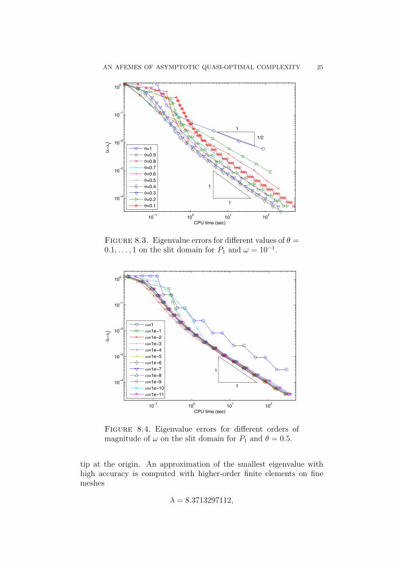
Figure 8.3. Eigenvalue errors for different values of θ =0.1, . . . , 1 on the slit domain for P1 and ω = 10−1.

10 1 100 101 102

10 4

10 3

10 2

10 1

100

CPU time (sec)

|l|

1

1

=1=1e 1=1e 2=1e 3=1e 4=1e 5=1e 6=1e 7=1e 8=1e 9=1e 10=1e 11

Figure 8.4. Eigenvalue errors for different orders ofmagnitude of ω on the slit domain for P1 and θ = 0.5.

tip at the origin. An approximation of the smallest eigenvalue withhigh accuracy is computed with higher-order finite elements on finemeshes

λ = 8.3713297112,


10 2 10 1 100 101 102 10310 5

10 4

10 3

10 2

10 1

100

CPU time (sec)

|l|

11/3

1

1

ARPACK uniformARPACK AFEMARPACK AFEMESLOBPCG AFEMESPINVIT AFEMES

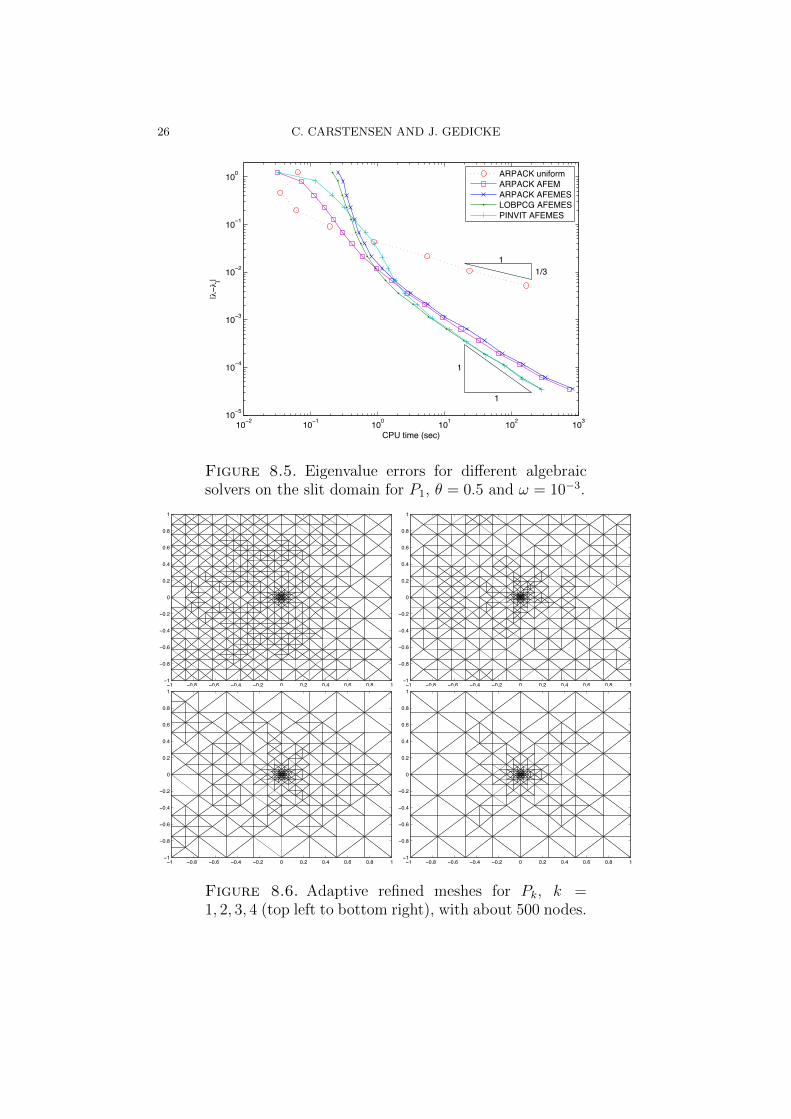
Figure 8.5. Eigenvalue errors for different algebraicsolvers on the slit domain for P1, θ = 0.5 and ω = 10−3.

1 0.8 0.6 0.4 0.2 0 0.2 0.4 0.6 0.8 11

0.8

0.6

0.4

0.2

0

0.2

0.4

0.6

0.8

1

1 0.8 0.6 0.4 0.2 0 0.2 0.4 0.6 0.8 11

0.8

0.6

0.4

0.2

0

0.2

0.4

0.6

0.8

1

1 0.8 0.6 0.4 0.2 0 0.2 0.4 0.6 0.8 11

0.8

0.6

0.4

0.2

0

0.2

0.4

0.6

0.8

1

1 0.8 0.6 0.4 0.2 0 0.2 0.4 0.6 0.8 11

0.8

0.6

0.4

0.2

0

0.2

0.4

0.6

0.8

1

Figure 8.6. Adaptive refined meshes for Pk, k =1, 2, 3, 4 (top left to bottom right), with about 500 nodes.


where the authors believe that all digits except the last one are exact.

Note that for uniform meshes and n = 2 it holds that N−1/2` ≈ h`.

Thus, for Pk, k = 1, . . . , 4, convergence rates of O(t−k` ) are optimal forthe eigenvalue error of the AFEMES. For the following experimentsthe PINVIT algebraic eigenvalue solver is used and the parametersare θ = 0.5 and ω = 10−3. The algorithm stops when a toleranceof 10−9 in the eigenvalue error is reached due to the accuracy of thereference eigenvalue or the number of degrees of freedom exceeds 106.In Figure 8.1 it is shown that the error estimator is numerically reliableand efficient for uniform meshes but these meshes result in suboptimal

convergence rates of about O(t−1/2` ) due to the singularity at the origin.

Note that the same rates are obtained for N` instead of t`. Thus thecomputational costs are quasi-optimal for uniform meshes. In contrastusing adaptive refinement results in experimental optimal convergencerates of O(t−k` ), k = 1, . . . , 4, as shown in Figure 8.2 and the errorestimator shows to be numerically reliable and efficient.

The asymptotic quasi-optimal AFEMES involves two parametersω > 0 and 0 < θ ≤ 1 which have to be sufficiently small. Figure 8.3shows a numerical strong dependency of the size of the eigenvalue erroron θ for ω = 0.1. For θ = 1 uniform refinement results in suboptimalconvergence rates. Smaller values lead to optimal convergence ratesand down to θ = 0.4 the error decreases. Then for even smaller valuesfor θ, the convergence rates are numerically optimal, but θ 1 leads tomore iterations of the algebraic eigenvalue solver and thus to more com-putational work. Note that for values θ ≤ 0.2 the algorithm marks toofew elements such that the algorithm accepts the value of the previouslevel as approximation for the next one from time to time. This resultsin the effect that those convergence plots look like a stair. Differentvalues for ω lead almost all (asymptotically) to optimal convergencerates as depicted in Figure 8.4. Only the value ω = 1 is not smallenough. The computational costs for smaller values only moderatelyincreases.

The asymptotic quasi-optimal complexity of AFEMES depends onthe choice of the algebraic eigenvalue solver. Figure 8.5 shows thatthe AFEMES is in the long term faster than one solve of ARPACK onan uniform mesh for linear P1 finite elements (“ARPACK uniform”).The results obtained with the multigrid preconditioned PINVIT andLOBPCG solver show asymptotic quasi-optimal computational com-plexity. The AFEMES shows larger computational time for ARPACKthan for PINVIT and LOBPCG due to the use of matrix factorisationsinstead of multigrid and the convergence rate deteriorates for largernumber of unknowns because the time for the matrix factorisationsdominates the computational costs. PINVIT and LOBPCG with ma-trix factorisations would lead to similar large computational costs.


100 101 102 10310 10

10 8

10 6

10 4

10 2

100

102

104

CPU time (sec)

l2 , |l|

1

8/3

12/3

1

2 1

4/3

P1 | l| uniform

P1 l2 uniform

P2 | l| uniform

P2 l2 uniform

P3 | l| uniform

P3 l2 uniform

P4 | l| uniform

P4 l2 uniform

Figure 8.7. Eigenvalue errors and estimated errors forthe 11th eigenvalue on the cube for uniform meshes withθ = 1 and ω = 10−4.

Different adaptive refined meshes for Pk, k = 1, 2, 3, 4, with about500 nodes are displayed in Figure 8.6. Note that the meshes arestrongly refined towards the corner singularity at the origin.

Example 8.2. Consider the three-dimensional model eigenvalue prob-lem (1.1) on the cube Ω = (0, 1)× (0, 1)× (0, 1) for the 11th eigenvalueλ11 = 12π2 which is simple. Note that for uniform meshes and n = 3

it holds that N−1/3` ≈ h`. Thus, for Pk, k = 1, . . . , 4, convergence

rates of O(t−2k/3` ) for the eigenvalue error are optimal. The asymp-

totic quasi-optimal AFEMES is stopped when 106 degrees of freedomare reached because of hardware limitations. Figure 8.7 shows opti-

mal convergence rates for uniform meshes of O(t−2k/3` ), k = 1, . . . , 4,

computing the 11th eigenvalue with the AFEMES using the LOBPCGsolver. The 11th eigenvalue is computed without any shift but from asubspace iteration.

Example 8.3. Consider the three-dimensional model eigenvalue prob-lem (1.1) on the L-shaped domain Ω = ((−1, 1)3)\([0, 1]2×[−1, 1]). Thefirst eigenvalue is the sum of π2 and the first eigenvalue of the two-dimensional L-shaped domain with approximation 9.6397238440219[BT05],

λ = 19.509328245111

(all displayed digits are correct). The asymptotic quasi-optimal AFEMESis stopped when 106 degrees of freedom are reached. In this non-convex


10 1 100 101 102 103

10 3

10 2

10 1

100

101

CPU time (sec)

l2 , |l|

1

4/9

P1 | l| uniformP1 l

2 uniform

P2 | l| uniformP2 l

2 uniform

P3 | l| uniformP3 l

2 uniform

P4 | l| uniformP4 l

2 uniform

Figure 8.8. Eigenvalue errors and estimated errorson the three-dimensional L-shaped domain for uniformmeshes with θ = 1 and ω = 10−3.

10 1 100 101 102 10310 6

10 5

10 4

10 3

10 2

10 1

100

101

102

CPU time (sec)

l2 , |l|

1

2/3

1

1

14/3

14/9


2 adaptive


2 adaptive


2 adaptive


2 adaptive

P4 | l| uniform

Figure 8.9. Eigenvalue errors and estimated errorson the three-dimensional L-shaped domain for adaptivemeshes with θ = 0.5 and ω = 10−3.

three-dimensional example uniform refinement results in suboptimal

convergence rates O(t−4/9` ) as shown in Figure 8.8. Note that the same

rates are obtained for N`. Note that the AFEMES is based on isotropicrefinement and therefore cannot create anisotropic meshes. Thus, we


10 1 100 101 102 103 10410 2

10 1

100

CPU time (sec)

|l|

1

2/3

1

2/5

1

4/9

ARPACK uniformARPACK AFEMARPACK AFEMESLOBPCG AFEMESPINVIT AFEMES

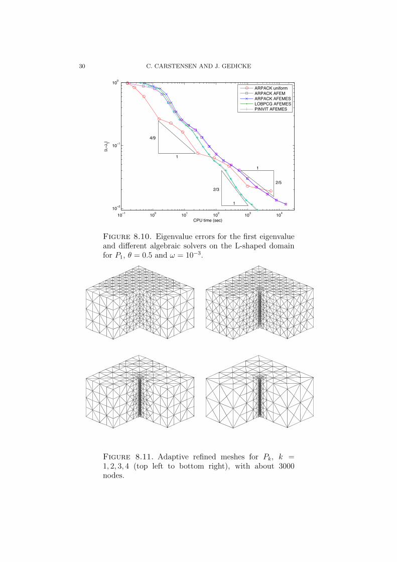
Figure 8.10. Eigenvalue errors for the first eigenvalueand different algebraic solvers on the L-shaped domainfor P1, θ = 0.5 and ω = 10−3.

Figure 8.11. Adaptive refined meshes for Pk, k =1, 2, 3, 4 (top left to bottom right), with about 3000nodes.


do not expect similar optimal rates for adaptively refined meshes as forthe two-dimensional case due to the edge singularity. This is no contra-diction to the theory because the definition of the approximation spacesinvolves only all possible isotropic and no anisotropic refinements. Forisotropic refinement for domains with edges [Ape99, Section 4.2] statesthe optimal relation N` ≈ h−3

` for linear P1 and the suboptimal re-

lations N` ≈ h−3` |lnh`| for P2, N` ≈ h

−2/9` for P3 and N` ≈ h

−1/6`

for P4 finite elements. Therefore, isotropic meshes are not optimal for

Pk, k ≥ 2 and convergence rates of O(t−2/3` ) for P1, rates slightly less

that than O(t−4/3` ) for P2 and rates of O(t

−4/3` ) for P3 and P4 are the

best possible for isotropic refinements. Figure 8.9 shows that the as-ymptotic quasi-optimal algorithm AFEMES with the PINVIT solver,θ = 0.5 and ω = 10−3 leads to these rates and that the error estimatoris reliable and efficient for Pk, k = 1, . . . , 4.

The computational time for the complete AFEMES with linear fi-nite elements is faster compared to one uniform solve with ARPACKas shown in Figure 8.10 for larger degrees of freedom. For smallernumbers of unknowns the computational costs for the assembly of thematrices and the calculation of the error estimator dominates and theconvergence rate of ARPACK uniform is the best possible for uniformmeshes but deteriorates for larger systems because of the computa-tion of the matrix factorisations. Since the computational costs forthe matrix factorisations get more severe for n = 3 and larger numberof degrees of freedom, this example shows that ARPACK with ma-trix factorisations leads to suboptimal computational complexity evenfor adaptively refined meshes. The PINVIT and the LOBPCG solverwith multigrid preconditioner lead to almost the same quasi-optimalcomplexity. Note that both graphs almost cover each other.

Different adaptive refined meshes for Pk, k = 1, 2, 3, 4, with about3000 nodes are displayed in Figure 8.11. The meshes are stronglyrefined towards the edge singularity for the higher-order methods.

Acknowledgements

The authors would like to thank the anonymous referees for theirvaluable comments and suggestions.

References

[ACF99] J. Alberty, C. Carstensen, and S.A. Funken, Remarks around 50 linesof Matlab: short finite element implementation, Numer. Algorithms 20(1999), no. 2-3, 117–137.

[AMP00] D.N. Arnold, A. Mukherjee, and L. Pouly, Locally adapted tetrahedralmeshes using bisection, SIAM J. Sci. Comput. 22 (2000), no. 2, 431–448.

[AO00] M. Ainsworth and J.T. Oden, A posteriori error estimation in finiteelement analysis, Pure and Applied Mathematics, Wiley-Interscience,New York, 2000.


[Ape99] T. Apel, Anisotropic finite elements: local estimates and applications,Advances in Numerical Mathematics, B. G. Teubner, Stuttgart, 1999.

[BDD04] P. Binev, W. Dahmen, and R. DeVore, Adaptive finite element methodswith convergence rates, Numer. Math. 97 (2004), no. 2, 219–268.

[Bre02a] S.C. Brenner, Convergence of the multigrid V -cycle algorithm forsecond-order boundary value problems without full elliptic regularity,Math. Comp. 71 (2002), no. 238, 507–525.

[Bre02b] , Smoothers, mesh dependent norms, interpolation and multigrid,Appl. Numer. Math. 43 (2002), no. 1-2, 45–56.

[BS08] S.C. Brenner and L.R. Scott, The mathematical theory of finite elementmethods, third ed., Texts in Applied Mathematics, vol. 15, Springer,New York, 2008.

[BT05] T. Betcke and L.N. Trefethen, Reviving the method of particular solu-tions, SIAM Rev. 47 (2005), no. 3, 469–491.

[CG11] C. Carstensen and J. Gedicke, An oscillation-free adaptive FEM forsymmetric eigenvalue problems, Numer. Math. 118 (2011), no. 3, 401–427.

[CKNS08] J.M. Cascon, C. Kreuzer, R.H. Nochetto, and K.G. Siebert, Quasi-optimal convergence rate for an adaptive finite element method, SIAMJ. Numer. Anal. 46 (2008), no. 5, 2524–2550.

[Dor96] W. Dorfler, A convergent adaptive algorithm for Poisson’s equation,SIAM J. Numer. Anal. 33 (1996), no. 3, 1106–1124.

[DPR03] R.G. Duran, C. Padra, and R. Rodrıguez, A posteriori error estimatesfor the finite element approximation of eigenvalue problems, Math. Mod-els Methods Appl. Sci. 13 (2003), no. 8, 1219–1229.

[DRSZ08] W. Dahmen, T. Rohwedder, R. Schneider, and A. Zeiser, Adaptive eigen-value computation: complexity estimates, Numer. Math. 110 (2008),no. 3, 277–312.

[DXZ08] X. Dai, J. Xu, and A. Zhou, Convergence and optimal complexity ofadaptive finite element eigenvalue computations, Numer. Math. 110(2008), no. 3, 313–355.

[FPW11] S. Funken, D. Praetorius, and P. Wissgott, Efficient implementation ofadaptive P1-FEM in Matlab, Comput. Methods Appl. Math. 11 (2011),no. 4, 460–490.

[GG09] S. Giani and I.G. Graham, A convergent adaptive method for ellipticeigenvalue problems, SIAM J. Numer. Anal. 47 (2009), no. 2, 1067–1091.

[GM11] E.M. Garau and P. Morin, Convergence and quasi-optimality of adaptiveFEM for Steklov eigenvalue problems, IMA J. Numer. Anal. 31 (2011),no. 3, 914–946.

[GMZ09] E.M. Garau, P. Morin, and C. Zuppa, Convergence of adaptive finiteelement methods for eigenvalue problems, Math. Models Methods Appl.Sci. 19 (2009), no. 5, 721–747.

[KN03a] A.V. Knyazev and K. Neymeyr, Efficient solution of symmetric eigen-value problems using multigrid preconditioners in the locally optimalblock conjugate gradient method, Electron. Trans. Numer. Anal. 15(2003), 38–55.

[KN03b] , A geometric theory for preconditioned inverse iteration. III. Ashort and sharp convergence estimate for generalized eigenvalue prob-lems, Linear Algebra Appl. 358 (2003), 95–114.


[Kny10] A. Knyazev, lobpcg.m,http://www.mathworks.com/matlabcentral/fileexchange/48-lobpcg-m,25 May 2000 (Updated 14 Mar 2010).

[LSY98] R.B. Lehoucq, D.C. Sorensen, and C. Yang, ARPACK users’ guide: So-lution of large-scale eigenvalue problems with implicitly restarted arnoldimethods, SIAM, Philadelphia, PA. USA, 1998.

[MM11] V. Mehrmann and A. Miedlar, Adaptive computation of smallest eigen-values of self-adjoint elliptic partial differential equations, Numer. LinearAlgebra Appl. 18 (2011), no. 3, 387–409.

[Ney02] K. Neymeyr, A posteriori error estimation for elliptic eigenproblems,Numer. Linear Algebra Appl. 9 (2002), no. 4, 263–279.

[Sau10] S. Sauter, hp-finite elements for elliptic eigenvalue problems: error es-timates which are explicit with respect to λ, h, and p, SIAM J. Numer.Anal. 48 (2010), no. 1, 95–108.

[SF73] G. Strang and G. J. Fix, An analysis of the finite element method,Prentice-Hall Inc., Englewood Cliffs, N.J., 1973, Prentice-Hall Seriesin Automatic Computation.

[Ste07] R. Stevenson, Optimality of a standard adaptive finite element method,Found. Comput. Math. 7 (2007), no. 2, 245–269.

[Ste08] , The completion of locally refined simplicial partitions created bybisection, Math. Comp. 77 (2008), no. 261, 227–241.

[SZ90] L.R. Scott and S. Zhang, Finite element interpolation of nonsmoothfunctions satisfying boundary conditions, Math. Comp. 54 (1990),no. 190, 483–493.

[Ver96] R. Verfurth, A review of a posteriori error estimation and adaptivemesh-refinement techniques, Wiley and Teubner, 1996.

(C. Carstensen) Humboldt-Universitat zu Berlin, Unter den Linden6, 10099 Berlin, Germany; Department of Computational Science andEngineering, Yonsei University, 120–749 Seoul, Korea.

E-mail address: [email protected]

(J. Gedicke) Humboldt-Universitat zu Berlin, Unter den Linden 6,10099 Berlin, Germany.

E-mail address: [email protected]

Documents

An Adaptive Finite Element Eigenvalue Solver of …gedicke/preprints/CG_2012.pdf · AN ADAPTIVE FINITE ELEMENT EIGENVALUE SOLVER OF ... lustrates the asymptotic quasi-optimal computational