An Aeroelastic Analysis of a Thin Flexible Membrane · An Aeroelastic Analysis of a Thin Flexible Membrane Robert C. Scott and Robert E. Bartelsy NASA Langley Research Center, Hampton,

An Aeroelastic Analysis of a Thin FlexibleMembrane

Robert C. Scott∗ and Robert E. Bartels†

NASA Langley Research Center, Hampton, VA, 23681, USA

Osama A. Kandil‡

Old Dominion University, Norfolk, VA, 23529, USA

Studies have shown that significant vehicle mass and cost savings are possible withthe use of ballutes for aero-capture. Through NASA’s In-Space Propulsion program, apreliminary examination of ballute sensitivity to geometry and Reynolds number wasconducted, and a single-pass coupling between an aero code and a finite element solverwas used to assess the static aeroelastic effects. There remain, however, a variety ofopen questions regarding the dynamic aeroelastic stability of membrane structures foraero-capture, with the primary challenge being the prediction of the membrane flut-ter onset. The purpose of this paper is to describe and begin addressing these issues.The paper includes a review of the literature associated with the structural analysis ofmembranes and membrane flutter. Flow/structure analysis coupling and hypersonic flowsolver options are also discussed. An approach is proposed for tackling this problemthat starts with a relatively simple geometry and develops and evaluates analysis meth-ods and procedures. This preliminary study considers a computationally manageable2-dimensional problem. The membrane structural models used in the paper include anonlinear finite-difference model for static and dynamic analysis and a NASTRAN finiteelement membrane model for nonlinear static and linear normal modes analysis. Bothstructural models are coupled with a structured compressible flow solver for static aeroe-lastic analysis. For dynamic aeroelastic analyses, the NASTRAN normal modes are usedin the structured compressible flow solver and 3rd order piston theories were used withthe finite difference membrane model to simulate flutter onset. Results from the variousstatic and dynamic aeroelastic analyses are compared.

Introduction

NASA’s new space exploration initiative has set anew course to develop human and robotic tech-

nologies that can deliver payloads larger than Apolloto the Moon, to Mars, and bring astronauts and sam-ples safely back to Earth at costs much lower thanApollo. These challenges require creative aerospacesystems. One proposed technology for safely deliver-ing payloads to the surface of Mars and return samplesto Earth involves flexible, deployable, perhaps inflat-able decelerators like ballutes.

Studies have shown that significant vehicle massand cost savings are possible with the use of ballutesfor aerocapture.1 These deployable decelerators canbe grouped into two general categories: trailing andclamped. The trailing ballute is characterized by aninflatable structure (typically a torus or sphere) con-nected to the payload aeroshell by tension lines. Onesuch concept is shown in figure 1. For the clampedballute, fabric fills the space between payload aeroshell

∗Senior Aerospace Engineer, Aeroelasticity Branch, AIAAAssociate Fellow.†Senior Aerospace Engineer, Aeroelasticity Branch.‡Professor, Department of Aerospace Engineering, AIAA As-

sociate Fellow.

Circular Torus

Cable

Fig. 1 Trailing ballute.

and the inflatable structure (torus). A concept for aclamped ballute is shown in figure 2.

Through NASA’s In-Space Propulsion (ISP) pro-gram,2 a preliminary examination of ballute sensitivityto geometry and Reynolds number and the influence oflarge displacements on aeroheating and dynamic pres-sures was conducted. Computational Fluid Dynamic(CFD) studies have investigated the interaction of thespacecraft wake and aeroheating and their sensitivities

1 of 17

American Institute of Aeronautics and Astronautics Paper 2007-2316

https://ntrs.nasa.gov/search.jsp?R=20070018292 2018-06-19T17:52:31+00:00Z

Circular Torus

Membrane

Fig. 2 Attached or clamped ballute.

to geometric and Reynolds number variations.3 Thesestudies have revealed that various types of favorableand unfavorable shock interactions exist for the dif-ferent ballute concepts.4 In addition, a single-passcoupling between an aero code and a finite elementsolver was used in reference 4 to assess static aeroe-lastic effects. It was found that the deformed shapeallows for a circulation pattern within the flexibletrough between the nose and the trailing edge. Thisdeformation resulted in local increases and decreasesin temperature and pressure along the aeroshell outerwall. Unsteady flow regions were also noted in some ofthe analyses. Aeroelastic stability was not considered.

A series of high speed wind-tunnel tests were alsoperformed as part of the ISP program.5 Severalwind-tunnel models were built out of plastic supportstructure and polyimide membranes to represent anattached ballute concept. Several membrane thick-nesses and cone angles were tested up to Mach 10 andReynolds number just over 525,000/foot. Some of themodels exhibited significant unsteadiness and in somecases, flutter resulting in dynamic failure of the mem-brane. These results underscore the need to predictthe static and dynamic aeroelastic response of thesemembrane structures.

Linear aeroelastic analysis methods are well under-stood and have long been applied to the aeroelasticanalyses of relatively stiff lifting surfaces. Virtuallyall current aircraft, as well as, spacecraft such as thespace shuttle have used these methods. Here, boththe structure and flow field are analyzed using lineartheories. The next level of improvement in fidelityof these methods is the use of nonlinear flow solvers,and a wide variety of CFD codes are available for thesubsonic, supersonic, and hypersonic flight regimes.The use of a linear structural theory with a nonlin-ear CFD flow solver is adequate provided the structureis still relatively stiff and behaves linearly to the ap-plied aeroloads. For ballutes and other membranestructures, aeroelastic analysis methods applicable tolinear structures are not adequate. Nonlinear struc-tural analysis methods are required.

The development of aeroelastic analysis methods for

ballutes will involve several technical challenges: 1)modeling the complex nonlinear behavior of a mem-brane; 2) coupling a highly flexible structure to CFDcodes; 3) the use of hypersonic flow solvers that havenot previously been used for aeroelastic analysis; 4)validation of the structural modeling and the aeroe-lastic analysis method. Because of these challengesthere have been very few aeroelastic analyses examin-ing membrane structures.

There are many open questions regarding the dy-namic aeroelastic analysis of ballutes and membranestructures. These questions include determining if anonlinear structural analysis close-coupled to a suit-able flow solver is required or whether a linear normalmodes structural model similarly coupled is adequateto assess dynamic stability? What are the implicationsof static pressure difference and tension on membranestability? How should the membrane be modeled if itis to be coupled with a flow solver? What are the timeaccuracy requirements of the hypersonic flow solver?Is the problem quasisteady/quasistatic with respect tothe flow? The purpose of this paper is to begin thework of answering these questions. This preliminarystudy will consider a computationally manageable 2-dimensional problem. The following will be discussed:

• Review of the literature associated with the struc-tural analysis of membranes, membrane flutter,and hypersonic flow solver options.

• A proposed approach to tackling this problemthat starts with a relatively simple geometry.

• A membrane finite difference model and discus-sion of model performance and convergence.

• Static analysis and comparison with a NASTRANnonlinear solution.

• Static aeroelastic analyses.

• Preliminary dynamic aeroelastic analyses.

• Concluding remarks that include a discussion ofaccomplishments and deficiencies in this study aswell as next steps.

Membrane Literature ReviewThis section of the paper will provide a review of

the literature associated with the structural analysisof membranes, membrane flutter, and hypersonic flowsolver options

Membrane Structural Analysis

The purpose of this section of the paper is to reviewthe various ways in which membranes have been an-alyzed for various types of engineering problems. Itis by no means a complete survey of the membrane

2 of 17


structural analysis. References 6 and 7 provide a moredetailed survey of nonlinear membrane analysis.

In the engineering field, the term membrane is re-served for zero bending rigidity structures. As withmost areas of engineering the mechanics of membranesencompasses the use of both linear and nonlinear mod-els. The applicability of the linearity assumption isvery problem dependent. One such linear problemis the analysis of a stretched string or cable. Thisproblem is essentially the same as the 2-dimensionalmembrane problem. The linearizing assumptions arethat the out-of-plane displacements are small and thetension in the string remains close to its equilibriumvalue.8 These assumptions result in a linear, constant-coefficient partial differential equation that has beenused directly in some of the earlier membrane flut-ter analyses. Unfortunately, the small deflection andconstant tension assumptions are not likely to be ap-plicable to the membrane flutter problem of a ballute.

Civil engineering has produced some work in thearea of membrane analysis. One such problem is theanalysis of guy cables. The study in reference 9 utilizeda time-domain finite element approach to study largeamplitude cable vibrations due to turbulent winds.Reference 10 considered the stability of a cable in in-compressible flow where the bulk of the stability anal-ysis was performed assuming constant tension. Othercivil engineering membrane applications include mem-brane roofs and inflatable or pneumatic structures.11

While clearly nonlinear, such problems are primarilystatic in nature considering a constant velocity wind.Transient response to wind loads has also been consid-ered but aeroelastic stability has not.

The aerodynamic analysis of sails is also relevant tothe study at hand, and there exist several papers onaerodynamic sail theory.12–15 Typically these studiesconsider the sail to be an inextensible membrane forwhich a static shape and associated lift coefficient issought. There have been some unsteady analyses, butaeroelastic stability had not been considered.

Somewhat similar to the analysis of sails is the studyof membrane wings for micro air vehicles. Shyy et alhave provided a number of papers on this topic.16–23

This work has focused on several key areas includ-ing the computation of aerodynamic coefficients, wingshape optimization, and aeroelastic response to tur-bulence and wind gusts. A key outcome of this workhas been the development of approaches for coupledmembrane-fluid dynamics analysis.

Another area where membranes have received con-siderable study has been the analysis of gossamerstructures like space sails and scientific balloons.24–33

Some studies of gossamer structures have used com-mercial codes like NASTRAN and ABAQUS. Onefinding of these studies is that this class of mem-

brane problems, where the membrane is initially un-derrestrained, can be very difficult to analyze usingfinite element methods. Reference 7 has an excellentdiscussion on the difficulties of analyzing membranestructures that undergo large displacements duringloading. This type of structural system is undercon-strained and stable equilibrium conditions only existfor loading fields that are orthogonal to the set of un-strained degrees of freedom. A common theme in theliterature is that achieving a converged static nonlin-ear solution can be a challenge.

One of the real challenges of analyzing a membranestructure is that it tends to wrinkle as it can’t sus-tain a compressive load. Considerable effort in recentyears has been applied to enhance membrane model-ing capabilities including membrane wrinkling, creasesdue to folds, and a variety of edge constraints, aswell as nonlinear thermal effects. Methods of analy-sis and models that incorporate these effects are beingdeveloped within NASATRAN, ABAQUS, and otherresearch codes.34

Obtaining a nonlinear static solution serves only asthe first step in obtaining a flutter solution. A pos-sible next step could be to use the stiffness matricesfrom a converged nonlinear static solution in a linearnormal modes analysis. The resulting normal modescould be used within CFD codes in the usual man-ner. Reference 31 describes one such procedure forMSC/NASTRAN in which a nonlinear static solutionfor an inflatable structure is obtained then a linearnormal modes analysis is performed. This approachdescribed in reference 31 will be used in this study.

Membrane Flutter Analysis

While there are many papers on panel flutter anda variety of research efforts continues in this area,35,36

there are but a handful of papers that specifically ad-dress membrane flutter. Some of these studies considerthe membrane flutter problem to be a limiting case ofa plate as bending rigidity approaches zero or inplanetension approaches infinity. In discussing the effectof in-plane stress on panel flutter speed, Blisplinghoffand Ashley37 stated that for the limiting case of amembrane, when in-plane force approaches infinity,the flutter speed is infinite. Reference 38 presents astudy of supersonic membrane flutter by consideringthe case of a two-dimensional plate in the presence ofchordwise tensile in-plane stresses as the plate bendingrigidity approaches zero. Reference 39 also consideredthe limiting case of a thin plate in supersonic flow.The analysis of reference 40 began with the membraneequation of a two dimensional membrane with a con-stant tension force and supersonic static aerodynamicapproximation. One of the results of these studies hasbeen the development of approximate flutter design

3 of 17


criterion, but the applicability of these criteria to theballute problem is limited, to say the least, due to thefact that these membranes were flat, linear, employedlinear/simplified aerodynamic theories, and neglectedstatic pressure difference across the membrane.

Hypersonic Flow Solver Options

Hypersonic panel flutter and hypersonic vehicleaeroservoelastic stability have been addressed throughwell established hypersonic aeroelastic analyses. Theaerodynamic theories for these analyses has typicallybeen classical or generalized linear and nonlinear pis-ton theory, hypersonic small disturbance theory or theperturbed Euler method.41,42 These methods requirethe assumptions of a thin body and sharp leadingedge and can be reasonably applied to lifting sur-faces or sharp nosed bodies of revolution. Ballutes arebluff bodies and clearly violate these assumptions, thusthese types aerodynamic theories are only suitable forpreliminary examination of membrane flutter analysisstrategies where the flow is approximately parallel tothe membrane surface.

The ballute operating environment will span therarified to continuum flow regimes, however, the high-est loading is expected to be within the continuumflow regime. For dynamic aerothermoelastic analysis,there are a number of codes that can be consideredfor this effort. Two open source codes available fromNASA Langley are LaURA43 and FUN3D.44 Thesecodes have the appropriate aerothermodynamic mod-els including equilibrium, non-equilibrium chemistryand surface catalycity. LaURA is not currently timeaccurate nor does it have a dynamic mesh capabil-ity. FUN3D is time accurate and has a dynamic meshcapability, and a modal capability has been recentlyadded.

Another open source code available from NASALangley is CFL3D.45–47 While this code lacks theaerothermodynamic analysis capabilities cited above,it is time accurate and has dynamic mesh and modalcapabilities. While chemistry models would need tobe added for accurate aerothermodynamic analysis,CFL3D may be suitable for initial assessment of closecoupled membrane flutter analysis strategies.

Flow/Structure Coupling

The primary goal of this study is the prediction ofthe membrane flutter onset. This will require that ap-propriate aerodynamic theories or codes be coupledwith a suitable structural analysis tool. The com-putational strategies can be grouped into essentiallytwo broad categories: 1) Loose coupling, and 2) Closecoupling. This section of the paper will provide abrief discussion of these approaches. In general, thesame types of flow and structural solvers can be used

in both strategies. Typically, a loose coupled anal-ysis is solved with the flow and structural parts ofthe problem in disparate domains. If time accuracyis preserved, close coupled analysis can also solve theflow and structure in disparate domains, or alterna-tively, the governing equations can be combined andthe problem solved simultaneously. The decision tocombine all parts of the analysis into a single code isoften based on convenience or, in the case of commer-cial codes, the availability of the source code. Theprimary difference between the two approaches is thatloose coupling is not time accurate while close couplingis. This means that a loose coupled strategy is suit-able for static aeroelastic calculations only, while closecoupling can be used for static or dynamic analyses.Table 1 lists the similarities and differences betweenthe two strategies. For a more detailed discussion ofcomputational approaches see reference 48.

Table 1 Flow/Structure coupling strategies.

Feature Loose Coupled Close CoupledTime Accurate No Yes

Flow/Struct- Disparate DisparateDescretization Unified

Flow Solver Any Any

Struct Solver Linear LinearNonlinear Nonlinear

Code Separate* SeparateCombined Combined*

Flow/Struct- Interpolated* InterpolatedInterface Same Grid Same Grid

Aeroelasticity Static StaticDynamic

*Typical

This paper will describe several modeling and anal-ysis procedures. These include: 1) A finite differencemodel coupled with CFD for static aeroelastic analy-sis; 2) A finite difference model coupled with pistontheory for static and dynamic aeroelastic analysis; 3)A NASTRAN finite element model coupled with CFDfor static aeroelastic analysis; and 4) A modal struc-tural model coupled with CFD for dynamic aeroelasticanalysis. It will be helpful and descriptve to discusswhere each of these fits into the loose/close couplingframework described above.

A finite difference structural model of a membranewill be described. This structural model is nonlin-ear and will be used with CFL3D in a loosely coupled

4 of 17


manner for static aeroelastic calculations in which theCFD surface grid and the structural grid are not co-incident and interpolation is used to pass informationbetween the two domains. This nonlinear structuralmodel will also be used with piston theory in a closecoupled manner in which the structure is nonlinearand solved simultaneously with the aerodynamics onthe same grid.

A finite element model (FEM) will also be describedin which two solution procedures will be used: nonlin-ear static and linear normal modes. For the staticaeroelastic analysis, this FEM will be used with anonlinear static solution procedure and loosely cou-pled with CFL3D for static aeroelastic calculations inwhich the CFD surface grid and the structural gridare not coincident and interpolation is used to passinformation between the two domains. Following thenonlinear static solution, the FEM will be used witha linear normal modes solution procedure to gener-ate natural frequencies and mode shapes that will bepassed via interpolation to CFL3D. Here the flow andmodal structural model are solved in a close coupledmanner within the same code, but in disparate do-mains. Here, the dynamic structural analysis is linear.

ApproachThe dynamic aeroelastic analysis of a thin-film bal-

lute will be a complex task. To determine flutter onset,a time marching close-coupled solution of the hyper-sonic flow field and structural dynamics of a detailedthin-film structural model may be required. The struc-tural analysis will be nonlinear and may also need tobe capable of modeling wrinkles. It is hoped that amodal approach may be adequate, but a fully coupledanalysis or experimental data will be needed to deter-mine if and when the modal approach can be used.This study will attempt to improve our understandingof aeroelastic membrane analysis by studying the sim-plest possible configuration. The following steps areproposed:

• Develop Finite Difference (FD) membrane struc-tural model including first order piston theoryaerodynamics. Evaluate stability and conver-gence properties of scheme. An advantage of theFD model is it may be relatively easy to add itto an existing CFD code. It may also be usefulor necessary to develop a nonlinear time accuratemembrane finite element model as an alternativeapproach, but this approach was not taken in thepresent study.

• Statically validate FD structural model with non-linear finite element analysis. This finite ele-ment analyses should include commercial codes

like NASTRAN, as well as, research codes. NAS-TRAN was used in the present study.

• Dynamically validate FD structural model withappropriate finite element analysis and theoreticalsolutions where available.

• Static aeroelastic analysis: Perform static aeroe-lastic analyses where Mach number, altitude,static pressure difference and pretension are var-ied. Examine convergence properties of the FDscheme.

• Static aeroelastic analysis: Perform static aeroe-lastic analyses where Mach number, altitude,static pressure difference and pretension are var-ied. Examine convergence properties of the FDscheme.

• Dynamic aeroelastic analysis: This should includefully coupled flutter analysis compared with amodal flutter analysis. The fully coupled anal-ysis will initially be the FD model but could alsoinclude a nonlinear time accurate finite elementanalysis.

• Apply higher fidelity aerodynamic methods tothe 2-dimensional membrane problem. Initially,the CFL3D code is used as it has all the nec-essary features for the aforementioned compari-son: time-accuracy, aeroelastic grid deformationscheme, and a modal capability. Later this couldinclude an appropriate hypersonic code.

• Examine a 3-dimensional, nominal flat membraneusing piston theory.

• Examine a 3-dimensional, nominal flat membraneusing CFL3D and other hypersonic CFD codes.

• It is hoped that this building block approach couldeventually lead to the development of an anal-ysis capability and suitable experience base forthe analysis and design of a 3-dimensional ballutestructure.

Finite Difference Membrane ModelThe problem considered in this study will be that

of a 2-dimensional membrane in the presence of super-sonic flow. The problem is shown in figure 3 and lookssimilar to the classical panel flutter problem. Themembrane properties to be considered in this studyare listed below,

E 800, 000 psiL 10 inh 0.001 inρm 0.0015945 slug/in3

5 of 17


L

x

M∞>>1y Membrane

h

Flow

Fig. 3 Two dimensional membrane.

ds

τ

∆p

θL

θR

TL

TR

i -1

i

i

i +1

θi

Fig. 4 Membrane model and membrane segmentforces.

Structural Equations of Motion

The linear equation for a 2-d membrane is

ρmh∂2w

∂t2− T

∂2w

∂x2+ ∆p = 0 (1)

Here, deformation in the x-direction is ignored and they-direction or out-of-plane deformation (w) is assumedsufficiently small that the tension (T ) is approximatelyconstant. The natural frequencies of this system areobtained by separation of variables with the pressuredifference across the membrane set to zero (∆p = 0)where n = 1, 2, 3, ...

fn =n√

Tρmh

2L(2)

This result will be used for some comparisons betweenthe FD scheme and linear theory later in the paper.

For the case of nonlinear equations of motion forthe membrane, we consider the balance of forces ofthe membrane segment shown in figure 4. Here, in thex-direction we obtain the following,

−TL cos θL + TR cos θR −∆p ds sin θi+τ ds cos θi = ρm h ds x (3)

and for the y-direction,

−TL sin θL + TR sin θR + ∆p ds cos θi+τ ds sin θi = ρm h ds y (4)

where,

cos θL =xi − xi−1√

(xi − xi−1)2 + (yi − yi−1)2(5)

cos θR =xi+1 − xi√

(xi+1 − xi)2 + (yi+1 − yi)2(6)

sin θL =yi − yi−1√

(xi − xi−1)2 + (yi − yi−1)2(7)

sin θR =yi+1 − yi√

(xi+1 − xi)2 + (yi+1 − yi)2(8)

ds =12

√(xi+1 − xi−1)2 + (yi+1 − yi−1)2 (9)

cos (θi) =12 (xi+1 − xi−1)

ds(10)

sin (θi) =12 (yi+1 − yi−1)

ds(11)

To simplify expressions that will appear later in thispaper we define the membrane length on the left andright of the ith point as,

`Li =√

(xi − xi−1)2 + (yi − yi−1)2 (12)

`Ri =√

(xi+1 − xi)2 + (yi+1 − yi)2 (13)

If the membrane material is linear elastic, the leftand right tension terms for the ith membrane segmentcan be approximated as,

TLi =

Eh

√(xi − xi−1)2 + (yi − yi−1)2 −∆xo(1− α ∆ T )

∆xo(14)

TRi =

Eh

√(xi+1 − xi)2 + (yi+1 − yi)2 −∆xo(1− α ∆ T )

∆xo(15)

6 of 17


where ∆xo is the undeformed or initial length of theith membrane segment. The term α ∆T representsthe thermal expansion coefficient and the temperaturechange that, for this implementation, are selected ar-bitrarily to obtain a desired value of pretension in themembrane. Only positive values of tension are permit-ted, so negative values are set to zero, and the abilityof this modeling approach to capture wrinkling is anopen question.

The nonlinear model to be developed in this sec-tion of the paper will be based on finite differenceexpressions. Finite difference representations for theacceleration of the ith point in the x and y directionsare

xi =xn+1i − 2xni + xn−1

i

(∆t)2(16)

and,

yi =yn+1i − 2yni + yn−1

i

(∆t)2(17)

where ∆t is the time step. Using these and the expres-sions developed previously, an implicit finite differenceexpression can be developed. Equations 3 and 4 canbe rewritten as shown in equations 18 and 19 (see bot-tom of next page) where,

ν =(∆t)2

ρm h ∆x(20)

The parameter ν has the appearance of a Courantnumber used in the Courant-Friedrichs-Lewy (CFL)condition that defines scheme stability limits on timestep and spatial mesh spacing. Equations 18 and 19form tridiagonal matrices that can be solved usingThomas’s algorithm.

Finite Element Membrane ModelAs mentioned earlier, one of the objectives of this

study is to assess the applicability of using a modalapproach for membrane and ultimately thin film bal-lute flutter analysis. While research codes may havethe latest algorithms and other unique capabilities,they often lack the library of elements and featuresnecessary to model complex structures. As such, NAS-TRAN will be utilized here as it has the capability toperform nonlinear static solutions and then perform amodal restart to obtain linear mode shapes and fre-quencies for conventional flutter analysis.

The membrane finite element model is shown in fig-ure 5. It is modeled using CQUAD4 elements withsuitable boundary conditions and properties to achieve2-dimensional behavior. The membrane material ismodelled as orthotropic with the Poisson ratio and thez-direction thermal expansion coefficient set to zero.

X

Y

Z

X

Y

Z

Fig. 5 NASTRAN membrane model.

X

Y

Z

1.13+00

0.

1.13+00

1.06+00

9.81-01

9.05-01

8.30-01

7.55-01

6.79-01

6.04-01

5.28-01

4.53-01

3.77-01

3.02-01

2.26-01

1.51-01

7.55-02

0. default_Fringe :Max 1.13+00 @Nd 57Min 0. @Nd 1 default_Deformation :Max 1.13+00 @Nd 57

MSC.Patran 2003 r2a 20-Dec-05 18:46:10

Fringe:SC2:DELTAP0.1, A1:Non-linear: 200. % of Load: Displacements, Translational-(NON-LAYERED) (MAG)

Deform:SC2:DELTAP0.1, A1:Non-linear: 200. % of Load: Displacements, Translational

X

Y

Z

Fig. 6 NASTRAN nonlinear static solution,∆Po = 2.5 psi and Pretension = 2 lbf/in.

The NASTRAN nonlinear static solution (SOL 106)essentially performs a series of analyses where the loadis incrementally increased to the desired level. It wasfound here that since the membrane is initially flat andvery thin a very small load increment is required atthe start of the analysis or the solution will fail. Oncethere is some deformation in the membrane due to thestatic pressure load, the membrane stiffness increasesand a larger load increment can be applied. As withthe finite difference model, the pretension is includedin the analysis via an arbitrary value of thermal ex-pansion coefficient and temperature change. Figure 6shows an example of a converged NASTRAN SOL 106(nonlinear static) solution.

Preliminary Static and DynamicMembrane Analyses

The purpose of this section of the paper is to presentthe results of the authors attempts to learn how to usethe finite difference membrane model described earlier.This is done prior to the introduction of aerodynamicforces. Stability, convergence, and dynamic behaviorof the finite difference membrane model are consid-ered. Finite difference analyses are compared withlinear theory or finite element analyses for the purpose

7 of 17


of validation.The analyses of the membrane comprises two

phases: obtaining a converged static solution followedby a dynamic analysis. The solution procedure forboth phases is largely the same; a time-marching anal-ysis is conducted until convergence is obtained or inthe case of the dynamic analysis, until stability can beassessed. In either case, scheme stability is a concernand the ν parameter identified earlier in equation 20is similar to the Courant number commonly encoun-tered in numerical schemes. A similar parameter wasidentified in reference 18 where a similar but less gen-eral modeling approach was taken. Typically, thereare upper limits on the value of ν for scheme stability.

For the values of h and ρm considered here, ∆x washeld constant at 0.5 in, and ∆t was varied to iden-tify an upper limit for scheme stability. A value of10−6 was ultimately found to be approximately theupper limit for stability. Inclusion of sub-iterationsin future versions of this finite difference model mayallow for larger time steps. For the flat membrane,the static converged solution is not necessary, but aninitial displacement perturbation is required. For thisand subsequent analyses, the initial deflection for thedynamic finite difference analyses is

yinitial = ystatic + 0.001 [sin(xπ/L)+sin(2xπ/L) + sin(3xπ/L)] (21)

where ystatic is the converged static solution. For thespecial case of ∆P = 0, the membrane is flat andystatic is zero.

Figure 7 shows the time history traces of all themembrane segment centers for the case of a flat mem-brane (∆P = 0). Here, we can see that the solutionis stable but has little damping. Spectral analysis ofthese time traces was performed to identify natural fre-quencies. These frequencies are listed in table 2 wherethey are compared with the theoretical linear frequen-cies (equation 2). While not identical, the frequenciesare consistent and indicate that no obvious implemen-tation errors are present in the finite difference model.

The lack of significant damping previously identifiedis good in the sense that the numerical scheme appears

2

1

0

-1

-2

1.0

0.5

0

-0.5

-1.0

x 10−3

x 10−6

y, in

0 0.004 0.008 0.012 0.016 0.020

Time, s

(x − x ), ininitial

Fig. 7 Time histories of membrane segment cen-ters for a flat membrane, ∆x = 0.05 in, ∆P =0.0 psi, and Pretension = 10 lbf/in.

Table 2 Comparison of modal frequencies (Hz.)for a flat membrane. ∆P = 0 psi andPretension = 10 lbf/in.

Mode Linear Theory Finite Difference1 475 4302 950 8593 1,425 1,289

to not be adding any, but the lack of damping is un-desirable in terms of obtaining a statically convergedsolution. An additional concern in getting a convergedstatic solution is the small size of the time step thatmust be used. Fortunately, for static solutions thereare a couple of obvious ways that convergence can beimproved. One way is to add some type of real orartificial damping to minimize dynamic oscillations.Using first-order-accurate estimates of the membranesegment center velocities in the x and y directions, thefollowing terms are added to the right hand side ofequations 18 and 19 to add damping,

0.035νxni − xn−1

i

∆t(22)

xn+1i+1 ν

(TnRi`nRi

+τ

2

)+ xn+1

i

(ν

(−TnLi`nLi

−TnRi`nRi

)− 1)

+ xn+1i−1 ν

(TnLi`nLi

− τ

2

)= −2xni + xn−1

i + ν∆p12

(yi+1 − yi−1)

(18)

yn+1i+1 ν

(TnRi`nRi

+τ

2

)+ yn+1

i

(ν

(−TnLi`nLi

−TnRi`nRi

)− 1)

+ yn+1i−1 ν

(TnLi`nLi

− τ

2

)= −2yni + yn−1

i − ν∆p12

(xi+1 − xi−1)

(19)

8 of 17


0 1 2 3 4 5 6 7 8 9 10

1.0

0.5

y, in

0 0.005 0.010 0.015 0,020

Time, sec

x, in

0.025 0.030 0.035 0.040

1.0

0.5

0.04

0.02

0

-0.02

-0.04

y, in

∆ x, in

Fig. 8 Converged membrane solution and time his-tories of membrane segment centers obtained withartificial structural damping and material density,∆x = 0.05in, ∆P = 1.0 psi, and Pretension =2.5 lbf/in.

0.035νyni − yin−1

∆t(23)

The other way to increase convergence is to artificiallyincrease the value of the material density so that alarger time step can be used for a given value of ν.This is a viable option as ρm does not influence thestatic solution, so the density can be increased by sev-eral orders of magnitude allowing the time step sizeto be similarly increased. With these modifications, aconverged static solution is easily obtained as shownby the membrane segment center time traces in fig-ure 8. For subsequent dynamic analysis, the dampingterms must be eliminated and nominal value of den-sity must be used. These methods of improving staticconvergence will be used throughout the remainder ofthis paper.

To further validate the finite difference model, con-verged static analyses can be compared with convergedNASTRAN SOL 106, nonlinear static solutions. Forthe finite difference and NASTRAN analyses, the fi-nal converged solutions for the case of ∆P = 1.0 psiand Pretension = 5 lbf/in are shown in figure 9. TheNASTRAN and the finite difference solutions are all inexcellent agreement, further indicating that the finitedifference membrane model is valid.

The final comparison to be made in this section ofthe paper will be between the natural frequencies ofthe finite difference scheme with those obtained us-ing NASTRAN. In the case of the NASTRAN, theappropriate frequencies are obtained by performing aSOL 103, normal modes analysis, using the stiffnessmatrix from the appropriate converged SOL 106, non-linear static solution. The finite difference frequenciesare calculated by first obtaining a converged staticsolution, followed by a dynamic analysis using the

0 1 2 3 4 5 6 7 8 9 10

1.4

1.2

1.0

0.8

0.6

0.4

0.2

y, in

x, in

Finite Difference Scheme

NASTRAN Nonlinear Static

Fig. 9 Comparison of finite difference and NAS-TRAN SOL 106 membrane displacement, ∆P =2.5 psi and Pretension = 5 lbf/in.

methods described above. Then, spectral analysis ofthe time traces is used to identify modal frequencies.The first three frequencies using each analysis methodare shown in table 3. The excellent comparison furthervalidates the finite difference scheme.

Table 3 Comparison of modal frequencies (Hz.),∆P = 1.0 psi and Pretension = 10 lbf/in.

Mode NASTRAN Finite Difference1 825 8202 1,177 1,1723 1,792 1,797

Aerodynamic ModelingSo far, ∆P has been considered a static quantity.

Here and throughout the remainder of the paper, ∆Pwill be defined as the sum of an unsteady compo-nent and a static component (∆Po). The unsteadycomponent of ∆P is a function of the structural dis-placement of the membrane. Two methods will beused to calculate the unsteady part of ∆P : piston the-ory and CFD. Piston theory has the advantage that itis simple and can be easily incorporated into the finitedifference scheme already described. When properlyapplied, CFD analysis is more accurate than pistontheory, and codes like CFL3D can model structuraldynamics modally.

Piston theory is a simple inviscid unsteady aerody-namic theory that has been used extensively in su-personic and hypersonic aeroelasticity. It provides apoint-function relationship between the local pressureon the surface and the local fluid velocity normal tothe surface. The derivation of piston theory utilizesthe isentropic expression for the pressure on the sur-

9 of 17


face of a moving piston.

p(x, t)p∞

=(

1 +γ − 1

2vna∞

) 2γ(γ−1)

(24)

where γ is the ratio of specific heats and a∞ is the freestream sonic speed. The normal velocity is

vn =∂w

∂t+ V∞

∂w

∂x(25)

where w is the out of plane displacement. The expres-sion for piston theory is based on a binomial expansionof equation 24. A third order expansion can be writtenas follows49

p(x, t)− p∞ = p∞

[γ

(vna∞

)+γ(γ + 1)

4

(vna∞

)2

+γ(γ + 1)

12

(vna∞

)3]

(26)

For implementation into the finite difference scheme,equation 25 will be rewritten,

(vn)i =yni − yn−1

i

∆t+ V∞

yni+1 − yni−1

xni+1 − xni+1

(27)

and with the addition of a static pressure difference,the ∆P term in equations 3 and 4 is

∆p = (p(x, t)− p∞) + ∆po (28)

Equations 26, 27, and 28 can be easily included in thefinite difference model. Static and dynamic aeroelas-tic analysis using piston theory will be presented in asubsequent section of the paper.

The alternative approach for calculating ∆P isto use CFD. The CFD code CFL3D version 6.4(CLF3Dv6.4)45,46 will also be used in this study.CFL3D solves the time-dependent conservation lawform of the Reynolds-averaged Navier-Stokes equa-tions using a finite-volume approach. Upwind-biasingis used for the convective and pressure terms whilecentral differencing is used for the shear stress andheat transfer terms. Implicit time advancement is usedwith the ability to solve steady or unsteady flows. Inthis study, the Euler equations were solved. UsingMATLAB m-file scripts, CFL3D can be loosely cou-pled with both the finite difference and the NASTRANmembrane models for static aeroelastic analysis. Fordynamic aeroelastic analysis, CFL3D currently onlysupports a modal representation of structures, andMATLAB m-file scripts were again used to loosely con-nect the two codes. These procedures will be discussedin more detail in the sections that follow.

One final note about the aerodynamic model. In thisstudy, analyses will be performed at constant Mach

number with altitude being varied. An atmospheremodel, curve fit of a standard atmosphere,50 was usedto calculate the temperature and density associatedwith a given altitude so that dynamic pressure andfree stream velocity could also be calculated. Thisaerodynamic model was used throughout this study,with both piston theory and CFD.

Membrane Static AeroelasticityThis section of the paper will examine the static

aeroelastic behavior of 2-d membranes. First, a looseCFD coupling procedure will be described followed bya discussion of results.

Structural/CFD Coupling for Static Aeroelasticity

A procedure was implemented to loosely coupleCFL3D with both the NASTRAN or the finite dif-ference membrane model. For this analysis two proce-dures had to be developed. One was to pass the pres-sure coefficient data from the CFD output to the inputof the structural analysis. The other requires that theoutput of the structural analysis (nodal displacements)be passed to the CFD code. These procedures wereperformed using MATLAB scripts (m-files). The de-tails of these two procedures will be described here.

To transfer pressures to the structural analysis in-put, the pressure coefficients were read from a CFL3Doutput file (cfl3d.prout). These coefficients were con-verted to pressures using the dynamic pressure ap-propriate for the Mach number and altitude beingexamined, and the resulting pressures were then inter-polated to the structural mesh using linear interpola-tion. In the case of the finite difference analysis, thesefixed pressures were then used in the time-marchingmembrane solution. For the NASTRAN analysis, ascript was used to generate a bulk data file (.bdf) con-taining PLOAD2 cards. This pressure data file wasused in the NASTRAN SOL 106 analysis by way of aninclude statement in the main input deck.

To transfer the structural displacements to the CFDanalysis, a script was used to interpolate the struc-tural displacements to the CFD computational surfacegrid points. In the case of the finite difference model,the structural displacements are available within theMATLAB environment, and in the case of the NAS-TRAN solution, the displacements are read from the.f06 output file. The structural displacements are theninterpolated to the CFD grid points and written to thefile newsurf.p3d. Within the CFL3D input file, thekeyword idef ss is set to unity which forces CFL3D toread the newsurf.p3d file and deform the grid accord-ingly.

While the static analysis is relatively straight for-ward with the aforementioned procedures being re-peated one after the other until convergence, there area couple of additional items of interest that should

10 of 17


0 1 2 3 4 5 6 7 8 9 10

1.0

0.9

0.8

0.7

0.6

0.5

0.4

0.3

0.2

0.1

Time, seconds

y,

inches

NASTRAN Nonlinear Static − CFL3D

Finite Difference Scheme − CFL3D

Finite Difference Scheme − Piston Theory (3)rd Order

Finite Difference Scheme − Piston Theory (1)st Order

Fig. 10 NASTRAN nonlinear static aeroelastic so-lution and finite difference aeroelastic solution us-ing CFL3D and piston theory, M = 5.0, Altitude =60, 000feet, ∆Po = 1.0 psi, and Pretension =10 lbf/in.

be considered. One of these was the use of a relax-ation factor that governs the portion of the structuraldisplacement from each iteration that is carried for-ward. For the Mach number considered, no relaxationwas needed (relaxation was unity) for all the finite dif-ference/CFD analyses and for the NASTRAN/CFDanalyses when the altitude was at or above 60,000 feet.Below this altitude, the NASTRAN/CFD analyses re-quired a very small value of relaxation (0.05) to achieveconvergence. Finally, it should be pointed out that theCFD grids used here were relatively simple, so theywere all generated using a MATLAB script.

Static Aeroelastic Analyses

The first set of data to be examined will be a com-parison of all the static aeroelastic analysis methodsdescribed in this paper. This includes the finite differ-ence membrane model with both 1st and 3rd orderpiston theory and CFD. Results obtained from theNASTRAN/CFD procedure will also be considered.Figure 10 shows a comparison of the converged staticaeroelastic analyses of the various approaches at analtitude of 60,000 feet. A significant observation isthe continued excellent agreement between the NAS-TRAN SOL 106 and the finite difference analysis whenthe same aerodynamic method is used. It is alsonoted that piston theory provides results consistentwith CFL3D, and as expected, 3rd order piston the-ory provides a result closer to the CFD analysis thandoes 1st order piston theory. First order piston theorywill no longer be considered in this study.

Figure 11 shows the results of a series of finite dif-ference/piston theory static aeroelastic analysis forM = 5.0 where altitude is varied from 200,000 feetto sea level. The highest altitude conditions repre-

0 1 2 3 4 5 6 7 8 9 10

0.7

0.6

0.5

0.4

0.3

0.2

0.1

y,

inches

x, inches

200K

180K

160K

140K

120K

100K

80K

60K

40K

20K

0K

Altitude, ft

Fig. 11 Static aeroelastic solutions obtained us-ing the finite difference membrane model and3rd order piston theory aerodynamics, M = 5.0,Pretension = 10 lbf/in, ∆Po = 1.0 psi, and∆x = 0.05 in.

200K

180K

160K

140K

120K

100K

80K

60K

40K

20K

0K

Altitude, ft

0 1 2 3 4 5 6 7 8 9 10

0.7

0.6

0.5

0.4

0.3

0.2

0.1

y,

inches

x, inches

Fig. 12 NASTRAN nonlinear static aeroelasticsolution with CFL3D Euler aerodynamics, M =5.0, ∆Po = 1.0 psi, and Pretension = 10 lbf/in.

sent very low dynamic pressures and the solutionsare nearly symmetric and similar to those obtainedpreviously. As altitude is reduced, increasing the dy-namic pressure, the converged deflections appear toflatten out due to the increasing aerodynamic load. Atthe lowest altitudes, the deflected membrane appearswrinkled. The results from a similar series of NAS-TRAN/CFD static analysis are shown in figure 12.The trends are the same as those noted for the fi-nite difference/piston theory analysis, but no apparentwrinkling is noted at the lower altitudes.

Two CFD solutions and their respective grids areshown in figures 13 and 14. Here, the membrane occu-pies the lower surface between x = 0 and x = 10. Thegrid extends upstream and downstream of the mem-brane 8 grid points in each direction. The membranedeformation built into these grids was obtained withCFL3D coupled with NASTRAN, and they are thesame as the deformation shown in figure 10 at the

11 of 17


RHO

2.0

1.9

1.8

1.7

1.6

1.5

1.4

1.3

1.2

1.1

1.0

0.9

0.8

0.7

0.6

0.5

0.4

0.3

0.2

x, inches

y,

inches

0-4 5 10 14

10

5

0

Fig. 13 CFL3D static aeroelastic solution gridwith nondimensional density contours, M = 5,Altitude = 200, 000feet, ∆Po = 1.0 psi, andPretension = 10 lbf/in.

x,

inches

y,

inches

0-4 5 10 14

10

5

0

1.51.41.31.21.11.00.90.80.70.60.50.4

RHO

Fig. 14 CFL3D static aeroelastic solution gridwith nondimensional density contours, M = 5,Altitude = 60, 000feet, ∆Po = 1.0 psi, andPretension = 10 lbf/in.

200,000 and 60,000 feet altitudes. These contour plotsshow the existence of a dissipated shock wave at theleading edge of the membrane indicating the need fora more refined grid.

Membrane Dynamic AeroelasticityThis section of the paper will examine the dynamic

aeroelastic behavior of 2-d membranes. The dynamicaeroelastic analysis begins where the static aeroelasticanalysis ends. As has already been described, for agiven Mach number and altitude, a converged staticaeroelastic solution is obtained. Then, a second nu-merical simulation is performed with artificial damp-ing terms removed and the static aeroelastic solutionperturbed slightly to assess stability. If the oscilla-tions decay, then the solution is deemed stable, andif they diverge, the solution is deemed unstable. Inthe case of the finite difference membrane analysis,3rd order piston theory will be used with the sameanalysis procedure as has already been described. Asof this writing, a flutter analysis with CFL3D is only

performed modally although the capability exists todirectly couple a structural solver and CFL3D. Thus, aCFL3D/NASTRAN modal flutter analysis procedurewill be described next, followed by some preliminaryflutter analyses.

Modal Flutter Analysis Procedure

The modal flutter analysis procedure has many stepsthat can most easily be described in the following enu-merated list.

1. Obtain a converged, nonlinear static aeroelasticsolution using the previously described looselycoupled NASTRAN SOL 106 and CFL3D staticsolution procedure.

2. Perform a NASTRAN SOL 103 analysis (normalmodes analysis), using the final stiffness matrixfrom the preceding step.

3. Extract the frequencies and mode shapes from theNASTRAN SOL 103 output file. Put modal fre-quencies in CFL3D input file.

4. Create CFD grid with the membrane surface de-formed into the converged static aeroelastic shapefrom the final NASTRAN SOL 106 solution instep 1.

5. Perform CFL3D analysis (irestart=0) with modaldeformation turned off (moddfl=-1).

6. Extract converged generalized forces from theCFL3D output, put these values in the CFL3Dinput file as input parameter gf0. Since thestatic aeroelastic shape is built into the grid,this step ensures that the pressure forces and in-ternal stresses initially sum to zero so that nostatic aeroelastic deformation is obtained withinCFL3D.

7. Restart CFL3D (irestart=1) with modal deforma-tion turned off (moddfl=-1). After this run, netgeneralized forces should be near zero. Withoutthis step, a transient in the generalized force willbe introduced.

8. Restart CFL3D (irestart=1) with modal deforma-tion turned on (moddfl=0) and a large value ofmodal damping (damp=0.99). This will removeany generalized coordinate transient associatedwith the net generalized force not being identi-cally zero.

9. Restart CFL3D (irestart=1) with modal deforma-tion turned on (moddfl=0) , modal damping setto zero (damp=0.0), and a perturbation value forthe modal velocities (x0(2*n)=0.05). This step inthe procedure is where stability is determined.

12 of 17


0 50 100 150 200 250 300

1.0

0.8

0.6

0.4

0.2

0

-0.2

-0.4

-0.6

-0.8

-1.0

x 10−5

Nondimensional Time

Generalized

Coordinate

Amplitude

Step 5 Step 7 Step 8 Step 9

Mode 1

Mode 2

Mode 3

Mode 4

Mode 5

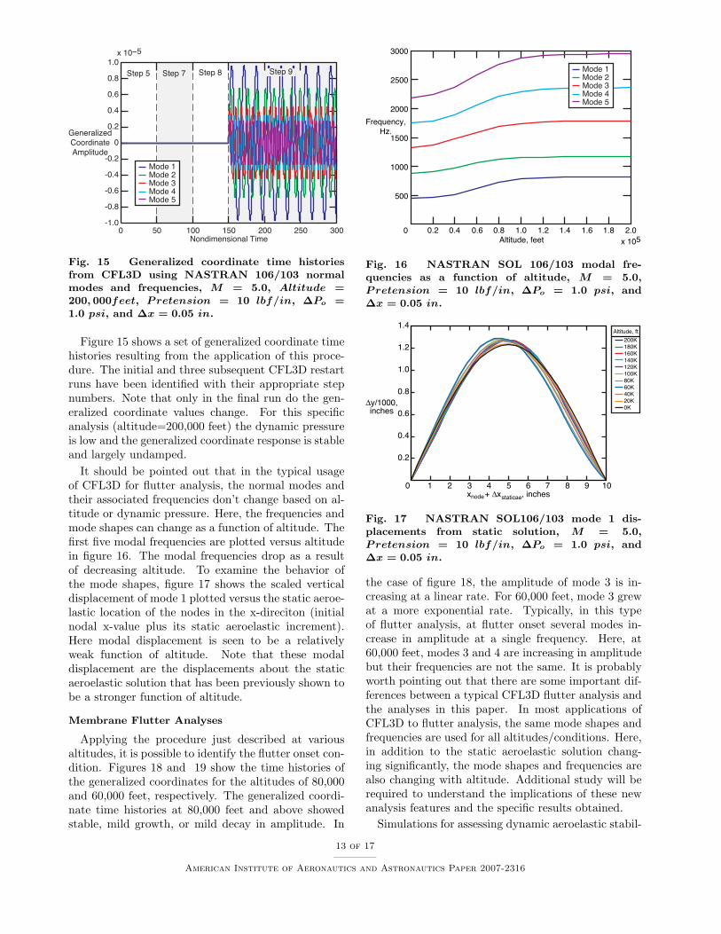
Fig. 15 Generalized coordinate time historiesfrom CFL3D using NASTRAN 106/103 normalmodes and frequencies, M = 5.0, Altitude =200, 000feet, Pretension = 10 lbf/in, ∆Po =1.0 psi, and ∆x = 0.05 in.

Figure 15 shows a set of generalized coordinate timehistories resulting from the application of this proce-dure. The initial and three subsequent CFL3D restartruns have been identified with their appropriate stepnumbers. Note that only in the final run do the gen-eralized coordinate values change. For this specificanalysis (altitude=200,000 feet) the dynamic pressureis low and the generalized coordinate response is stableand largely undamped.

It should be pointed out that in the typical usageof CFL3D for flutter analysis, the normal modes andtheir associated frequencies don’t change based on al-titude or dynamic pressure. Here, the frequencies andmode shapes can change as a function of altitude. Thefirst five modal frequencies are plotted versus altitudein figure 16. The modal frequencies drop as a resultof decreasing altitude. To examine the behavior ofthe mode shapes, figure 17 shows the scaled verticaldisplacement of mode 1 plotted versus the static aeroe-lastic location of the nodes in the x-direciton (initialnodal x-value plus its static aeroelastic increment).Here modal displacement is seen to be a relativelyweak function of altitude. Note that these modaldisplacement are the displacements about the staticaeroelastic solution that has been previously shown tobe a stronger function of altitude.

Membrane Flutter Analyses

Applying the procedure just described at variousaltitudes, it is possible to identify the flutter onset con-dition. Figures 18 and 19 show the time histories ofthe generalized coordinates for the altitudes of 80,000and 60,000 feet, respectively. The generalized coordi-nate time histories at 80,000 feet and above showedstable, mild growth, or mild decay in amplitude. In

0.2 0.4 0.6 0.8 1.0 1.2 1.4 1.6 1.8 2.0

x 105

0

3000

2500

2000

1500

1000

500

Altitude, feet

Frequency,

Hz.

Mode 1

Mode 2

Mode 3

Mode 4

Mode 5

Fig. 16 NASTRAN SOL 106/103 modal fre-quencies as a function of altitude, M = 5.0,Pretension = 10 lbf/in, ∆Po = 1.0 psi, and∆x = 0.05 in.

0 1 2 3 4 5 6 7 8 9 10

1.4

1.2

1.0

0.8

0.6

0.4

0.2

∆y/1000,

inches

x + ∆x , inches

Altitude, ft

200K

180K

160K

140K

120K

100K

80K

60K

40K

20K

0K

staticaenode

Fig. 17 NASTRAN SOL106/103 mode 1 dis-placements from static solution, M = 5.0,Pretension = 10 lbf/in, ∆Po = 1.0 psi, and∆x = 0.05 in.

the case of figure 18, the amplitude of mode 3 is in-creasing at a linear rate. For 60,000 feet, mode 3 grewat a more exponential rate. Typically, in this typeof flutter analysis, at flutter onset several modes in-crease in amplitude at a single frequency. Here, at60,000 feet, modes 3 and 4 are increasing in amplitudebut their frequencies are not the same. It is probablyworth pointing out that there are some important dif-ferences between a typical CFL3D flutter analysis andthe analyses in this paper. In most applications ofCFL3D to flutter analysis, the same mode shapes andfrequencies are used for all altitudes/conditions. Here,in addition to the static aeroelastic solution chang-ing significantly, the mode shapes and frequencies arealso changing with altitude. Additional study will berequired to understand the implications of these newanalysis features and the specific results obtained.

Simulations for assessing dynamic aeroelastic stabil-

13 of 17


100 140 180 220 260 300

1.5

1.0

0.5

0

-0.5

-1.0

-1.5

x 10−5

Nondimensional Time

Generalized

Coordinate

Amplitude

Mode 1

Mode 2

Mode 3

Mode 4

Mode 5

Fig. 18 Generalized coordinate time histories fromCFL3D using NASTRAN 106/103 normal modesand frequencies, M = 5.0, Altitude = 80, 000feet,Pretension = 10 lbf/in, ∆Po = 1.0 psi, and ∆x =0.05 in.

100 140 180 220 260 300

Nondimensional Time

Generalized

Coordinate

Amplitude

2.0

1.5

1.0

0.5

0

-0.5

-1.0

-1.5

-2.0

x 10−5

Mode 1

Mode 2

Mode 3

Mode 4

Mode 5

Fig. 19 Generalized coordinate time histories fromCFL3D using NASTRAN 106/103 normal modesand frequencies, M = 5.0, Altitude = 60, 000feet,Pretension = 10 lbf/in, ∆Po = 1.0 psi, and ∆x =0.05 in.

ity using the finite difference scheme coupled with 3rdorder piston theory were also performed at the variousaltitudes. Figure 20 shows the vertical displacementtime history for the approximate center point of themembrane (i=11) at the various altitudes. When thealtitude is 40,000 feet or greater the solution is stable.For altitudes of 20,000 feet and below the solutionsare unstable. The proper interpretation of this resultis, however, unclear. Initially, the response grows ina smooth manner. One might interpret this result asflutter onset, but due to the nonlinearities, a limit cy-

0 0.002 0.004 0.006 0.008 0.010

1.0

0.8

0.6

0.4

0.2

0

-0.2

-0.4

-0.6

-0.8

-1.0

y , in

Time, s

200K

180K

160K

140K

120K

100K

80K

60K

40K

20K

0K

Altitude, ft

11

Fig. 20 Time history of vertical displacement ofmembrane center point (yi=11) using finite differ-ence structural model and 3rd order piston theoryaerodynamics, M = 5.0, Pretension = 10 lbf/in,∆Po = 1.0 psi, and ∆x = 0.05 in.

cle oscillation (LCO) might be expected. Instead ofa ”stable” LCO, the solution blows up after a fewcycles. This problem may be associated with a lim-itation in the ability of the finite difference schemeto handle large geometric nonlinearities, and it shouldalso be noted that the static aeroelastic solutions as-sociated with the conditions where the ”instabilities”occurred showed some wrinkling-like behavior. If theexact point of instability onset is identified (between40,000 and 20,000 feet) a stable LCO may be obtained.

To summarize the flutter analyses performed so far,hard flutter onset is between 80,000 and 60,000 feetfor the CFL3D modal flutter analysis and between40,000 and 20,000 feet for the finite difference/pistontheory analysis. Also, at the intermediate altitudes(40,000 to 100,000 feet) a large amount of aerodynamicdamping is introduced in the finite difference/pistontheory analyses, while little or no aerodynamic damp-ing appears to be present for any of the CFL3D modalanalyses. Clearly, additional study will be requiredto fully understand membrane flutter and these pre-liminary results. It is also apparent that the viabilityof modal based flutter analysis versus a fully nonlin-ear structural simulation cannot yet be assessed, as theanalyses performed so far utilize different aerodynamicmethods.

Concluding RemarksThe aeroelastic analysis of a thin-film ballute is a

technical challenge. One of the challenges is the model-ing of the ballute’s complex, 3-dimensional membranestructure. A membrane with large deflections is non-linear and it has the tendency to wrinkle, complicatingboth the structural analysis as well as the associatedaerodynamic analysis. There are a number of possibleways to model the membrane including finite differ-ence, finite element, and modal representations. The

14 of 17


modal representation must be linearized about a non-linear static solution. Commercial finite element codesexist that can model membrane structures, but de-veloping a close-coupled aeroelastic analysis capabilitywill not be possible due to the proprietary nature ofthese codes. Aeroelastic analysis schemes based onclose and loose coupling with appropriate flow solverswill both need to be investigated to verify and validatethe various approaches.

This paper proposed a series of steps leading to thedevelopment of a membrane flutter analysis capabil-ity. A building block approach is proposed in whichincreasing levels of complexity are added. Initially,the simplest possible structural and aerodynamic mod-els are considered. This approach should allow for athorough understanding of the physics and numericsassociated with each step.

This paper examined a relatively simple, 2-dimensional membrane structure. A finite differencerepresentation of the membrane was developed thatcaptured membrane pretension and static pressure dif-ference across the membrane. This model was thenused to obtain nonlinear static solutions with variouslevels of pretension and static pressure difference. ANASTRAN membrane model was developed and non-linear static solutions were obtained and comparedwith those from the finite difference model. Thesestatic analyses were in excellent agreement. Addition-ally, some dynamic validation studies were also pre-sented. Here, frequencies from spectral analysis of thefinite difference time traces were compared with thefrequencies from linear theory and NASTRAN SOL106/103. These studies further validated the finite dif-ference membrane model.

Third order piston theory aerodynamics was in-cluded in the membrane finite difference model, anda series of static aeroelastic solutions was obtainedat various altitudes for fixed Mach number. At thelower altitudes, some of these solutions appeared wrin-kled. A procedure was developed to couple both theNASTRAN nonlinear static solution and the finite dif-ference scheme with CFL3D. Here, the NASTRANand finite difference solution were in excellent agree-ment.

Using the converged static aeroelastic solutions asa starting point, dynamic stability was investigated.Here again, altitude was varied for a fixed Mach num-ber with solution time histories being examined ateach condition. Two analyses types were considered:1) The membrane finite difference scheme with pis-ton theory aerodynamics, and 2) NASTRAN SOL 106and SOL 103 mode shapes and frequencies in CFL3D.At a fixed Mach number, both methods provided es-timates of the flutter onset altitude. In contrast tothe static analyses, these flutter analyses were not in

good agreement. The flutter onset altitudes were dif-ferent as were the damping characteristics of the timetraces as a function of altitude. Further study will berequired to fully understand the implications of thesepreliminary results.

There is clearly much additional work to be doneto gain a good understanding of the aeroelastic char-acteristics of thin membrane structure, and furtherstudy and method development will need to be per-formed to better understand the dynamic aeroelasticbehavior of thin membranes. This work includes CFDand structural grid convergence studies. Paramet-ric studies where the effects of membrane geometry,static pressure difference, and pretension are consid-ered. The finite difference equations need to be in-corporated into CFL3D to make a proper comparisonbetween structural modeling approaches, and the useof Navier Stokes equations in the flow solver shouldalso be considered. Ultimately, a hypersonic CFD flowsolver will need to be used.

References1Rohrschneider, R. R. and Braun, R. D., “A Survey of

Ballute Technology for Aerocapture,” Proceedings of the 3rd In-ternational Planetary Probe Workshop, June 2005.

2Johnson, L., Alexander, L., Baggett, R., Bonometti, J.,Herrmann, M., James, B., and Montgomery, S., “NASA’s In-Space Propulsion Technology Program: Overview and Update,”40th AIAA/ASME/SAE/ASEE Joint Propulsion Conferenceand Exhibit , No. AIAA-2004-3841, July 2004.

3Gnoffo, P. A. and Anderson, B. P., “Computational Anal-ysis of Towed Ballute Interactions,” 8th AIAA/ASME JointThermophysics and Heat Transfer Conference, No. AIAA 2002-2997, June 2002.

4Hornung, H. G., “Hypersonic Flow Over Bodies in Tandemand its Relevence to Ballute Design,” 31st AIAA Fluid Dynam-ics Conference, No. AIAA 2001-2776, June 2001.

5Buck, G. M., “Testing of Flexible Ballutes in Hyper-sonic Wind Tunnels for Planetary Aerocapture,” 44th AIAAAerospace Sciences Meeting and Exhibit , No. AIAA-2006-01319,Jan. 2006.

6Jenkins, C. H. and Leonard, J. W., “Nonlinear dynamicResponse of Membranes: State of the Art,” Applied MechanisReview , Vol. 44, No. 7, July 1991.

7Jenkins, C. H., “Nonlinear dynamic Response of Mem-branes: State of the Art - Update,” Applied Mechanis Review1996 Suplement , Vol. 48, No. 10, Oct. 1996.

8Main, I. G., Vibrations and Waves in Physics, 1993.9Sparling, B. F. and Davenport, A. G., “Nonlinear Dynamic

Behavior of guy Cables in Turbulent Winds,” Canadian Journalof Civil Engineering, Vol. 28, 2001, pp. 98–110.

10Anderson, W. J., “Dynamic Instability of a Cable in Incom-pressible Flow,” AIAA/ASME/SAE 14th Structures, StructuralDynamics, and Materials Conference, March 1973.

11de Oliveira Pauletti, R. M., Guirardi, D. M., and De-ifeld, T. E. C., “Argyris’ Natural Membrane Finite ElementRevisited,” International Conference on Textile Composites andInflatable Structures, Structural Membranes, 2005.

12Vanden-Broeck, J.-M., “Nonlinear Two-Dimensional SailTheory,” Physics of Fluids, Vol. 25, No. 3, March 1982.

13Maitre, O. L., Huberson, S., and Cursi, E. S. D., “Un-steady Model of Sail and Flow Interaction,” Journal of Fluidsand Structures, Vol. 13, 1999.

15 of 17


14Nielson, J. N., “Theory of Flexible Aerodynamic Surfaces,”Journal of Applied Mechanics, , No. 63-APM-29, 1963.

15Newman, B., “Aerodynamic Theory for Membranes andSails,” Progress in Aerospace Sciences, Vol. 24, 1987.

16Smith, R. and Shyy, W., “Computation of AerodynamicCoefficients for a Flexible Membrane Airfoil in Turbulent Flow:A Comparison with Classical Theory,” Physics of Fluids,Vol. 12, No. 8, Dec. 1996.

17Shyy, W. and Smith, R., “A Study of Flexible AirfoilAerodynamics with Application to Micro Aerial Vehicles,” 28thAIAA Fluid Dynamics Conference, No. AIAA-1997-1933, June1997.

18Lillberg, E., Kamakoti, R., and Shyy, W., “Computationof Unsteady Interaction Between Viscous Flows and FlexibleStructure with Finite Inertia,” 38th Aerospace Sciences Meetingand Exhibit , No. AIAA 2000-0142, Jan. 2000.

19Smith, R. and Shyy, W., “Computation of Unsteady Lam-inar Flow Over a Flexible Two-Dimensional Membrane Wing,”Physics of Fluids, Vol. 9, No. 7, Sept. 1995.

20Shyy, W. and Smith, R., “Computation of Laminar Flowand Flexible Structure Interaction,” Computational Fluid Dy-namics Review 1995 , 1995.

21Lian, Y., Shyy, W., Viieru, D., and Zhang, B., “Mem-brane Wing Aerodynamics for Micro Air Vehicles,” Progress inAerospace Sciences, 2003.

22Lian, Y., Shyy, W., and Haftka, R., “Shape Optimizationof a Membrane Wing for Micro Air Vehicles,” 41st AerospaceSciences Meeting and Exhibit , No. AIAA 2003-0106, Jan. 2003.

23Lian, Y., Shyy, W., and Ifju, P. G., “A ComputationalModel for Coupled Membrane-Fluid Dynamics,” 32nd AIAAFluid Dynamics Conference and Exhibit , No. AIAA 2002-2972,June 2002.

24Johnston, J. D., Blandino, J. R., and McEvoy, K.,“Analytical and Experimental Characterization of Gravity In-duced Deformations in Subscale Gossamer Structures,” 45thAIAA/ASME/ASCE/AHS/ASC Structures, Structural Dy-namics and Materials Conference, No. AIAA 2004-1817, April2004.

25Papa, A. and Pellegrino, S., “Mechanics of System-atically Creased Thin-Film Membrane Structures,” 46thAIAA/ASME/ASCE/AHS/ASC Structures, Structural Dy-namics and Materials Conference, No. AIAA 2005-1975, April2005.

26Tessler, A., Sleight, D. W., and Wang, J. T., “NonlinearShell Modeling of Thin Membranes with Emphasis on StructuralWrinkling,” 44th AIAA/ASME/ASCE/AHS/ASC Structures,Structural Dynamics and Materials Conference, No. AIAA2003-1931, April 2003.

27Lee, K. and Lee, S. W., “Structural Analysis of ScientificBalloons Using Assumed Strain Formulation Solid Shell FiniteElements,” 46th AIAA/ASME/ASCE/AHS/ASC Structures,Structural Dynamics and Materials Conference, No. AIAA2005-1802, April 2005.

28Woo, K. and Jenkins, C. H., “Global/Local Anal-ysis Strategy for Partly Wrinkled Membrane,” 46thAIAA/ASME/ASCE/AHS/ASC Structures, StructuralDynamics and Materials Conference, No. AIAA 2005-1977,April 2005.

29Sleight, D. W. and Muheim, D. M., “Parametric Stud-ies of Square Solar Sails Using Finite Element Analysis,”45th AIAA/ASME/ASCE/AHS/ASC Structures, StructuralDynamics and Materials Conference, No. AIAA 2004-1509,April 2004.

30Greschik, G., Palisoc, A., Cassapakis, C., Veal, G., andMikulas, M. M., “Sensitivity Study of Precision PressurizedMembrane Reflector Deformations,” AIAA Journal , Vol. 39,No. 2, Feb. 2001.

31Smalley, K. B., Tinker, M. L., and Fischer, R. T., “In-vestigation of Nonlinear Pressurization and Modal Restartin MSC/NASTRAN for Modeling Thin Film InflatableStructures,” 42nd AIAA/ASME/ASCE/AHS/ASC Structures,Structural Dynamics, and Materials Conference and Exhibit ,No. AIAA 2001-1409, April 2001.

32Sakamoto, H. and Park, K., “Design Parameter Ef-fects for Wrinkle Reduction in Membrane Space Structures,”46th AIAA/ASME/ASCE/AHS/ASC Structures, StructuralDynamics and Materials Conference, No. AIAA 2005-1974,April 2005.

33Sutjahjo, E., Su, X., Abdi, F., and Taleghani, B., “Dy-namic Wrinkling Analysis of Kapton Membrane Under TensileLoading,” 45th AIAA/ASME/ASCE/AHS/ASC Structures,Structural Dynamics and Materials Conference, No. AIAA2004-1738, April 2004.

34Tessler, A., Sleight, D. W., and Wang, J. T., “EffectiveModeling and Nonlinear Shell Analysis of Thin Membranes Ex-hibiting Structural Wrinkling,” Journal of Spacecraft and Rock-ets, Vol. 42, No. 2, April 2005.

35Dowell, E. H., “Panel Flutter: A Review of the AeroelasticStability of Plates and Shells,” AIAA Journal , Vol. 8, No. 3,1970.

36Mei, C., Abdel-Motagaly, K., and Chen, R., “Review ofNonlinear Panel Flutter at Supersonic and Hypersonic Speeds,”Applied Mechanics Reviews, Vol. 52, No. 10, 1999.

37Bisplinghoff, R. L. and Ashley, H., Principles of Aeroelas-ticity, 1962.

38Spriggs, J., Messiter, A., and Anderson, W., “Mem-brane Flutter Paradox-An Explanation by Singular Perturba-tion Methods,” AIAA Journal , Vol. 7, No. 9, Sept. 1969.

39Johns, D., “Supersonic Membrane Flutter,” AIAA Jour-nal , Vol. 9, No. 5, May 1971.

40Ellen, C., “Approximate Solutions of the Membrane Flut-ter Problem,” AIAA Journal , Vol. 3, No. 6, June 1965.

41Liu, D. D., Chen, P. C., Tang, L., and Chang, K. T., “Hy-personic Aerothermodynamics/Aerothermoelastics Methodol-ogy for Reusable Launch Vehicles/TPS Design and Analysis,”41st Aerospace Sciences Meeting and Exhibit , No. AIAA 2003-897, Jan. 2003.

42Hui, W. H. and Liu, D. D., “Unsteady UnifiedHypersonic-Supersonic Aerodynamics : Analytical and Ex-pedient Methods for Stability and Aeroelasticity,” 44thAIAA/ASME/ASCE/AHS Structures, Structural Dynamicsand Materials Conference, No. AIAA 2003-1964, April 2003.

43Gnoffo, P. A., McCandless, R. S., and Yee, H. C., “En-hancements to Program LAURA for Computation of Three-Dimensional Hypersonic Flow,” AIAA 25th Aerspace SciencesMeeting, No. AIAA 87-0280, Jan. 1987.

44Kleb, W. L., Nielsen, E. J., Gnoffo, P. A., Park, M. A., andWood, W. A., “Collaborative Software Development in Supportof Fast Adaptive AeroSpace Tools (FAAST),” 16th AIAA Com-putational Fluid Dynamic Conference, No. AIAA 2003-3978,June 2003.

45Krist, S. L., Biedron, R. T., and Rumsey, C. L., “CFL3DUser’s Manual (Version 5.0),” NASA-TM 1998-208444, June1998.

46Bartels, R. E., “CFL3D Version 6.4 General Usage andAeroelastic Analysis,” NASA-TM 2006-214301, 2006.

47McNamara, J. J., Friedmann, P. P., Powell, K. G.,Thuruthimattam, B. J., and Bartels, R. E., “Three-dimensional Aeroelastic and Aerothermoelastic Behavior in Hy-personic Flow,” 46th AIAA/ASME/ASCE/AHS/ASC Struc-tures, Structural Dynamics and Materials Conference, April2005.

48Bartels, R. E., Moses, R. W., Scott, R. C., Templeton,J. D., Cheatwood, F. M., Gnoffo, P. A., and Buck, G. M., “AProposed Role of Aeroelasticity in NASA’s New Exploration

16 of 17


Vision,” International Forum on Aeroelasticity and StructuralDynamics, No. IF-013, 2005.

49Libhthill, M. J., “Oscillating Airfoils at High Mach Num-ber,” Journal of Aeronautical Sciences, Vol. 20, No. 6, June1953.

50“Earth Atmosphere Model, Imperial Units,”http://www.grc.nasa.gov/WWW/K-12/airplane/atmos.html .

17 of 17


Documents

An Aeroelastic Analysis of a Thin Flexible Membrane · An Aeroelastic Analysis of a Thin Flexible Membrane Robert C. Scott and Robert E. Bartelsy NASA Langley Research Center, Hampton,