HAL Id: inria-00275461https://hal.inria.fr/inria-00275461

Submitted on 23 Apr 2008

HAL is a multi-disciplinary open accessarchive for the deposit and dissemination of sci-entific research documents, whether they are pub-lished or not. The documents may come fromteaching and research institutions in France orabroad, or from public or private research centers.

L’archive ouverte pluridisciplinaire HAL, estdestinée au dépôt et à la diffusion de documentsscientifiques de niveau recherche, publiés ou non,émanant des établissements d’enseignement et derecherche français ou étrangers, des laboratoirespublics ou privés.

An algebraic method for multi-dimensional derivativeestimation

Samer Riachy, Yara Bachalany, Mamadou Mboup, Jean-Pierre Richard

To cite this version:Samer Riachy, Yara Bachalany, Mamadou Mboup, Jean-Pierre Richard. An algebraic method formulti-dimensional derivative estimation. MED’08, 16th IEEE Mediterranean Conference on Controland Automation, Jun 2008, Ajaccio, Corsica, France. 2008. <inria-00275461>

An algebraic method for multi-dimensional derivative estimation

Samer Riachy, Yara Bachalany, Mamadou Mboup and Jean-Pierre Richard

Abstract— This communication revisits the algebra-basedresults for derivative estimation presented by Fliess and co-authors in 2005. It is proposed, here, to consider multi-dimensional functions, namely scalar or vector fields of severalvariables. Such fields are locally represented by a vector Taylorseries expansion, and a computation technique is presented soto put successive partial derivatives (for instance, the gradient,the Hessian matrix...) as functions of iterated integrals of themeasured quantities.

I. INTRODUCTION

Classical field theory [2] (not to be confused with algebraicfield theory) is a well developed branch of mathematics,suitable to describe phenomena with distributed parameterssuch as fluid mechanics, heat transfer, econometrics [10],optimization [3] and many others.

Basic ingredients of the field theory are operators suchas gradient vector, Jacobian, Laplacian, Hessian, divergence,curl, etc... Close looking to these operators, one can noticethat they are combinations of successive partial derivativesof the field (scalar or vector) with respect to its coordinates.

As stated above, distributed parameters systems are mod-eled as fields (scalar or vector), and the above mentionedoperators are manipulated in order to have a qualitative ideafor a given problem. If one seeks quantitative description,numerical simulations have to be done.

One of the major problems in numerical simulation is thedilemma of accuracy and computational cost in estimatingthe above operators.

As an example, consider the problem of edge detection inimage processing. Roughly speaking, an image is a scalarbidirectional field (x, y), and the problem of edge detectioncan be solved by computing the Laplacian at each of theimage pixels. The Laplacian operator is given by:

L =∂2

∂x2+

∂2

∂y2.

Thus estimating the Laplacian reduces to estimating secondorder partial derivatives with respect to x and y.

S. Riachy and Jean-Pierre Richard: Projet ALIEN, INRIAFUTURS and Equipe SyNeR, LAGIS UMR CNRS 8146,Ecole Centrale de Lille, P.O. Box: 48, Cite Scientifique, 59651Villeneuve d’Ascq, France. samer.riachy@ec-lille.fr,jean-pierre.richard@ec-lille.fr

Y. Bachalany: LAGIS, Universite des Sciences etTechnologies de Lille, 59651 Villeneuve d’Ascq, Franceyara.bachalany@ed.univ-lille1.fr

M. Mboup: Projet ALIEN, INRIA FUTURS and UFR de Mathematiqueset Informatiques, universite Rene Descartes (Paris 5) 45 rues dessaints-Peres, Paris cedex 06 France mboup@math-info.univ-paris5.fr

Usually those quantities are estimated with use of finitedifferences, resulting in poor estimation in the presence ofnoise.

In this paper, we propose a methodology whose purposeis to compute an estimate for successive partial derivativesof a given field.

Robust and fast time derivation of noisy signals is nowpossible, thanks to an algebra-based approach initiated in [7],and oriented toward signal derivation in [4], [5], [6], [8], [9].Advanced results on algebra-based derivative estimation canbe found in [9], which basic concepts well be recalled insection II.

Based on a truncated Taylor expansion, nth order deriva-tives are obtained through iterative integrations on the signal.

In [4], estimation of the derivatives of a multidimensionalsignal was considered. The estimator developed in [4] wasbased on a 2nd order bidimensional Taylor expansion, andwas constituted of a linear combination of the signal andits (first) integral. But, using the original signal (withoutintegration) may introduce perturbations in noisy cases. Inthis paper, we present a more general estimators based on amulitidimentional N th order Taylor expansion. We will seethat the resulting estimators are linear combination of iteratedintegration on the multidimensional signal.

A sufficiently smooth field can be locally represented byits vector Taylor expansion to the N th order. Consider atruncation to the N th order of some Cr, r ≥ 2, functionf(x) : U ⊆ Rn → R defined on some compact set U , withx = (x1, · · · , xn)T :

f(x + ∆x) = f(x) + G∆x + ∆xT H∆x + · · · , (1)

G =[

Ix1 . . . Ixn

],

H=

Ix2

1Ix1x2 . . . Ix1xn

Ix2x1 Ix22

. . . Ix2xn

......

. . ....

Ixnx1 Ixnx2 . . . Ix2n

.

The Ixi , Ix2i

i = 1 · · ·n are partial derivatives of f(x)with respect xi. On the one hand, they can be seen as the 1st

and 2nd derivative estimation of a mono-dimensional noisysignal. Thus the derivative estimation technique from [9] canbe used. Section (II) recalls its basic concepts. On the otherhand, a vector Taylor expansion is used to compute thosequantities. Section (III) presents some examples.

Generic forms can also be computed resulting in familiesof estimators. One of them is used for the estimation ofthe off-diagonal terms for the Hessian matrix. This is alsopresented in section (III).

In section (IV), a comparison with finite differencesmethod is provided for the computation of successive partialderivatives on an academic example.

II. NUMERICAL DIFFERENTIATION: A RECALL

This part recalls the framework introduced in [9]. Lety(t) = x(t) + n(t) be a noisy observation on a finite timeinterval of a real-valued signal x(t), the derivatives of whichare to be estimated. The signal x(t) is assumed to be analytic.It is known that an analytic signal can be expanded into aTaylor series:

x(t) =∑i≥0

x(i)(0)ti

i!.

On some finite interval of time, a truncation of theTaylor expansion to some order N is acceptable as a ‘good’approximation:

xN (t) =N∑

i≥0

x(i)(0)ti

i!, t ∈ [0, T ]. (2)

The successive derivatives estimation requires some math-ematical manipulation on (2) such as time derivation andintegration by parts. Doing these operations several times ina row is tedious and lengthy, while doing the same in theoperational domain reduces computation time and providesmore compact forms. For this reason, applying the Laplacetransform to (2) gives:

sN+1xN (s) = sNx(0) + sN−1x(0) + · · ·+ x(N)(0),

where xN (s) is the operational analog to xN (t) on [0, T ].To be able to calculate individual estimators for the nth

order derivative (see [9] for a detailed discussion on whatis called simultaneous and individual estimators and thedifference between), a properly chosen differential opera-tor is needed to annihilate all the remaining coefficientsx(j)(0), j ∈ 0, · · · , N − n. One differential operatorhas the form:

ΘN,nκ =

dn+κ

dsn+κ

1s

dN−n

dsN−nκ ≥ 0.

It yields the following estimator for xn(0) :

xn(0)sν+n+κ+1

=(−1)n+κ

(n + κ)!(N − n)!1sν

ΘN,nκ (sN+1x),

which is strictly proper whenever ν is of the form ν =N + 1 + µ, µ ≥ 0. A family of strictly proper estimatorsparameterized by κ, µ and N is obtained. Back to timedomain, one obtains:

x(n)N (0) =

(ν + n + κ)!(−1)n+κ

(n + κ)!(N − n)!T ν+n+κ

∫ T

0

Π(τ)x(τ)dτ,

with:

Π(τ) =

N−nXi=0

„N − n

i

«(N + 1)!

(n + i + 1)!

N+κXj=0„

n + κj

«(n + 1)!

(1 + j − κ)!

(T − τ)ν+κ−j−2(−τ)i+j

(ν + κ− j − 2)!.

As a concrete final form for the estimator, one may obtainafter normalization of the integral into [0, 1] forms like theones below:

It =−30T

∫ 1

0

(3− 32τ + 90τ2 − 96τ3 + 35τ4)f(Tτ)dτ,

for n = 1, N = 2, µ = 5, κ = 1.

It2 =336T 2

∫ 1

0

(4− 75τ + 360τ2 − 700τ3 + 600τ4

−189τ5)f(Tτ)dτ.

for n = 2, N = 3, µ = 6, κ = 1.

III. ESTIMATORS BASED ON THE VECTORTAYLOR EXPANSION

Consider the N th order vector Taylor series expansion forthe scalar field f(x). Note that the development in (1) maybe expressed in a more general form as:

f(x) =N∑

i=0

1i!

(n∑

k=1

xk∂

∂xk

)i

f(x)

x=0

, (3)

with:(∂i1

∂xi11

∂i2

∂xi22

· · · ∂in

∂xinn

)f(x) := I

xi11 x

i22 ···xin

n:= I

Πnl=1x

ill

,

i1 + i2 + · · ·+ il = i.

The multivariable Laplace transform is a linear operatoron a scalar field f(x) with x = (x1, . . . , xn)T ∈ Rn

+,transforming it into a scalar field f(s) with s =(s1, . . . , sn)T ∈ Cn and defined as follows:

f(s) =∫

Rn+

f(x) exp−sT x dx. (4)

We follow the same reasoning as in section (II). The ideais to try to put the desired partial derivative (to be estimated)as a function of iterated integrals of the observed quantities.Computation are far more complex than the one-dimensioncase in section (II). We start by some examples, to showhow to proceed and, then, we present a generic form for thecomputation of the off-diagonal terms of the Hessian matrix.

A. Introductory examples

Consider a scalar vector field depending on two variablesz = f(x, y). Its Taylor truncation (for N = 2) around (0, 0)is given by:

f2(x, y) = I(0, 0) + Ix(0, 0)x + Iy(0, 0)y +1

2Ix2(0, 0)x2

+1

2Iy2(0, 0)y2 + Ixy(0, 0)xy.

In the operational domain, and after omitting (0, 0) fromthe above equation, one obtains:

I(s, p) =I

sp+

Ix

s2p+

Iy

sp2+

Ix2

s3p+

Iy2

sp3+

Ixy

s2p2(5)

1) Estimation of the 1st derivative using a bidimentionalTaylor expansion: To compute Ix, we try to manipulate (5)so to isolate Ix. Start by multiplying (5) by s3p3 and thenderivate two times with respect to p and once with respectto s. Next multiply by 1

sp and differentiate once with respectto s. The right-hand side of (5) reduces to −2Ix

s2p . Applyingthe same operations to the left-hand side of (5) we obtain:

18I(s, p) + 30s∂I(s, p)

∂s+ 18p

∂I(s, p)∂p

+ 30sp∂2I(s, p)

∂s∂p

+3p2 ∂2I(s, p)∂p2

+ 5sp2 ∂3I(s, p)∂s∂2p

+ 6s2 ∂2I(s, p)∂s2

+6s2p∂3I(s, p)∂s2∂p

+ s2p2 ∂4I(s, p)∂s2∂p2

= −2Ix

s2p

Note that multiplying by s (or p) corresponds to derivatewith respect to x (or y) in the time domain, which is notdesirable. For this reason, multiply (6) by 1

s3p3 and thenapply the inverse transform (see appendix) to return backto time the domain. The following form is obtained:

184

∫ X

0

∫ Y

0

(X − x)2(Y − y)2I(x, y)dxdy +

302

∫ X

0

∫ Y

0

(X − x)(Y − y)2(−x)I(x, y)dxdy +

182

∫ X

0

∫ Y

0

(X − x)2(Y − y)(−y)I(x, y)dxdy +

30∫ X

0

∫ Y

0

(X − x)(Y − y)(−x)(−y)I(x, y)dxdy +

32

∫ X

0

∫ Y

0

(X − x)2(−y)2I(x, y)dxdy +

5∫ X

0

∫ Y

0

(X − x)(−x)(−y)2I(x, y)dxdy +

62

∫ X

0

∫ Y

0

(Y − y)2(−x)2I(x, y)dxdy +

6∫ X

0

∫ Y

0

(Y − y)(−x)2(−y)I(x, y)dxdy +∫ X

0

∫ Y

0

(−x)2(−y)2I(x, y)dxdy +

= −2IxX4

4!Y 3

3!.

After an appropriate change of variable to normalize theintegrals over the interval [0, 1], the final form is obtained:

Ix =−36X

∫ 1

0

∫ 1

0

(−48x− 36y − 160xy2

−180x2y + 9 + 30y2 + 45x2 + 150x2y2

+192xy)I(Xx, Y y)dxdy (6)

2) Estimation of the Ix2 , Ixy derivatives using a bidimen-tional Taylor expansion: Similarly, to compute an estimatorfor Ix2 , one has to manipulate (5) so to isolate Ix2 . One wayis to successively apply 1

s3p4∂2

∂s2∂2

∂p2 s3p3. The final form intime domain and after normalization of the integrals over[0, 1] is the following:

Ix2 =180X2

∫ 1

0

∫ 1

0

(−18x− 12y − 60xy2

−72x2y + 3 + 10y2 + 18x2 + 60x2y2

+72xy)I(Xx, Y y)dxdy. (7)

Similarly applying 1s3p3

∂∂p

∂∂s

1sp

∂∂p

∂∂ss3p3 on (5), we ob-

tain:

Ixy =144XY

∫ 1

0

∫ 1

0

(−240x2y − 48y − 48x

−240xy2 + 9 + 45y2 + 45x2 + 225x2y2

+256xy)I(Xx, Y y)dxdy. (8)

Note that (8) is symmetric in x and y.

B. Generic form for Ixiyj

The equivalent equation to (3) in the operational domainis obtained through the Laplace transform (4):

fN (S) =N∑

n=0

1n!

n!Πk

i=1sn+1i

[n∑

i1=0

n∑i2=n−i1

n∑i3=n−i2

· · ·

n∑ik−1=n−ik−2

k∏f=0

sif

f IΠk

f=0xn−iff

with ik = kN −

∑k−1l=1 il. The elementary Laplace trans-

formation used to obtain the above equation are shown inappendix.

To estimate Ixixji, j = 1, . . . , n, multiply by the

differential operator:

ΞN,n,i,jκ1,κ2

= Ω∏

l∈1,..,n−i,j

(∂N

∂sNl

),

with

Ω =∂κ1+1

∂sκ1+1

∂κ2+1

∂sκ2+1

1sisj

∂N−1

∂sN−1i

∂N−1

∂sN−1j

.

It yields the following estimator for Ixixj i, j = 1, . . . , n

Ixixj

sκ1+2i sκ2+2

j Πnl=1s

il

l

= α1

Πnl=1s

il

l

ΞN,n,i,jκ1,κ2

n∏l=1

(sN+1

l

)f(S),

with

α =(−1)κ1+κ2+2

(κ1 + 1)!(κ2 + 1)!(N !)n−2[(N − 1)!]2.

Similar generic forms for all terms in (3) can also becomputed.

IV. NUMERICAL SIMULATIONS

In order to show the efficiency of the above developed es-timators, simulations are achieved on a bidimensional signalgiven by f(x, y) = sin( 1

2x2+ 14y2+3)cos(2x+1−ey). The

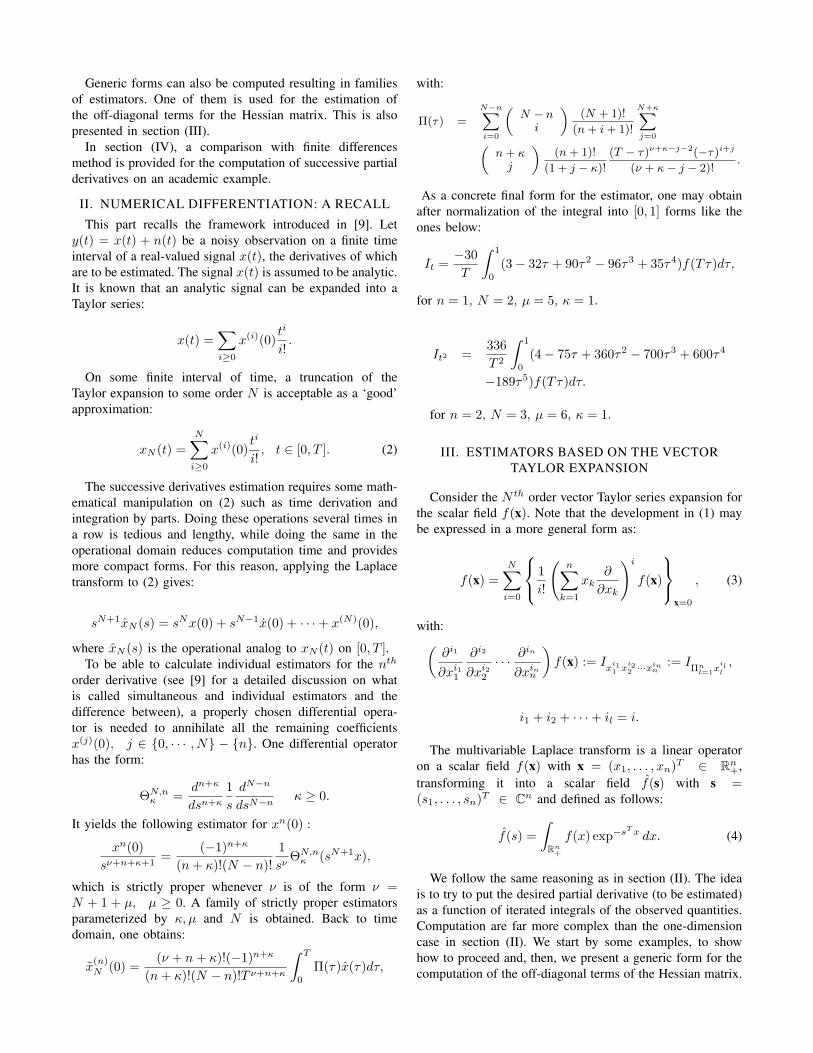
obtained results are compared with finite differences methodsfrom [1]. A step sampling of (0.001× 0.001) is used. As itis clear, estimators are computed on some elementary (non-infinitesimal) surface over [0, X]×[0, Y ] with X = Y = 0.06(for noise free simulations). Such surface involves 7×7 = 49samples.

Fig. 1. 3-D plot of f(x, y) = sin( 12x2 + 1

4y2 + 3)cos(2x + 1− ey)

The derivatives are computed at a point (xi, yi) with yi =2 and xi ranging from −2 to 7. In fact, at each point ofthe line (−2 ≤ xi ≤ 7, yi = 2), the elementary surfaceneeded for the computation is taken around the particularpoint (xi, yi).

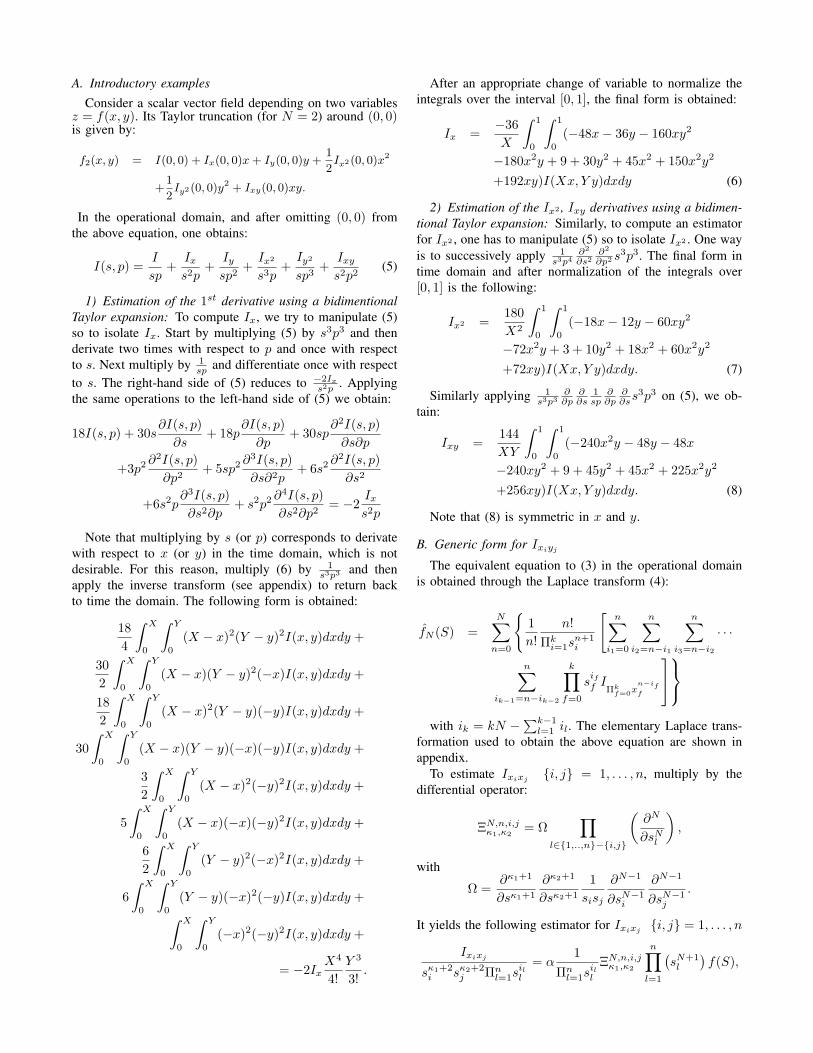
Simulation results are shown in figures (2) and (3). Thesecond order derivative (7) is plotted in a yellow thick line,while the finite differences ([1] section 25.3.23) is plotted ina red thin line in figure (2). Figure (3) shows the estimationof Ixy based on (8) in a thick yellow line and the finitedifferences from ([1] section 25.3.26) in a thin red line. Infigures (2) and (3) the formal derivatives are in dashed green.It is easily seen that the finite differences lacks curvature incomparison to the algebra-based derivative.

Next, the surface is corrupted with noise n(x, y). Thenoise level is measured by the signal to noise ratio in dB,

i.e., SNR = 10 log10

(Pi,j |f(xi,yj)|2Pi,j |n(xi,yj)2|

). In the following

simulation, the SNR is set to SNR = 25 dB. Figure (4)shows a slice of the noisy surface in the plane xi = 2 andfor yi ranging from −1 to 3.

Fig. 2. Estimation of Ix2

Fig. 3. Estimation of Ixy

Fig. 4. A slice of the noisy surface at xi = 2 and −1 < yi < 3, 25 dB

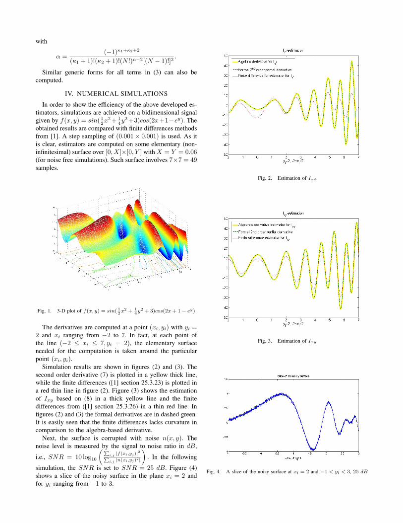
A comparison between the algebra-based, and finite dif-ference 1st derivative estimation are compared in figures(5) and (6) respectively. The elementary surface neededfor computation is of 80 × 80 samples. The same surfacedimension (80×80) is used in both cases. The algebra-basedapproach shows robustness with respect to noise. Note thatthe estimation in (5) is subject to a delay. Following thesame reasoning as in [9], an explanation through the Jacobipolynomials can be given. This is left for another work.

Fig. 5. Algebra-based estimation of the 1st derivative, Ix

Fig. 6. Finite difference estimation of the 1st derivative, Ix

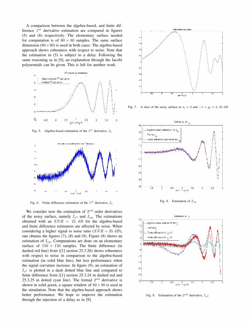
We consider now the estimation of 2nd order derivativesof the noisy surface, namely Ix2 and Ixy . The estimationsobtained with an SNR = 25 dB for the algebra-basedand finite difference estimators are affected by noise. Whenconsidering a higher signal to noise ratio (SNR = 35 dB),one obtains the figures (7), (8) and (9). Figure (8) shows anestimation of Ixy . Computations are done on an elementarysurface of 150 × 150 samples. The finite difference (indashed red line) from ([1] section 25.3.26) shows robustnesswith respect to noise in comparison to the algebra-basedestimation (in solid blue line), but less performance whenthe signal curvature increase. In figure (9), an estimation ofIx2 is plotted in a dash dotted blue line and compared tofinite difference from ([1] section 25.3.24 in dashed red and25.3.25 in dotted cyan line). The formal 2nd derivative isshown in solid green, a square window of 80×80 is used inthe simulation. Note that the algebra-based approach showsbetter performance. We hope to improve the estimationthrough the injection of a delay as in [9].

Fig. 7. A slice of the noisy surface at xi = 2 and −1 < yi < 3, 35 dB

Fig. 8. Estimation of Ixy

Fig. 9. Estimation of the 2nd derivative, Ix2

V. CONCLUSION

In this communication, we have presented an extensionof the algebra-based derivative to multidimensional signals.Based on a vector Taylor expansion and the multivariableLaplace transform, estimators are computed. Those estima-tors are iterated integrals over the observed multidimensionalsignal. Our estimators are compared to finite differencesmethods from the literature. As demonstrated in [9], the in-troduction of a delay in the estimators improves considerablythe quality of estimation and its robustness with respect tonoise. A similar reasoning is hoped to be attached to themultidimensional estimators.

VI. APPENDIX

A. Laplace transform

In transforming from time domain into the operationaldomain, the following Laplace transform is used:

L

(k∏

i=1

xnii

)=

k∏i=1

ni!sni+1

(9)

To demonstrate this transform, start first with k = 2 whichyields to:

L(xn

n!ym

m!) =

1sn+1

1pm+1

.

Suppose G(x, y) = xn

n!ym

m! with n, m ∈ Z. Then,∫ ∞

0

e−py

∫ ∞

0

e−sxG(x, y)dxdy

=∫ ∞

0

e−py

∫ ∞

0

e−sx xn

n!ym

m!dxdy

=∫ ∞

0

e−py ym

m!

∫ ∞

0

e−sx xn

n!dxdy

=∫ ∞

0

e−py ym

m!1

sn+1dy

=1

sn+1

∫ ∞

0

e−py ym

m!dy

=1

sn+1

1pm+1

.

The general formula (9) is easily deduced by recurrenceon xi.

B. Inverse transformBack to time domain this inverse-transform is used:

L−1

1Qk

i=1 snii

da1+···+akIQki=1 ds

aii

!=

1Qki=1(ni − 1)!

Z X1

0· · ·Z Xk

0

kYi=1

(Xi − xi)ni−1

kYi=1

(−xi)aiI(x1, x2, · · · , xk)dxk · · · dx1 (10)

To demonstrate this inverse-transform, start first with k = 2,which yields:

L−1(1sn

1pm

∂a+bI

∂sadpb)

Let G = ∂bI∂pb ,

1snpm

∂aG

∂sa=

1pm

1sn

∂aG

∂sa

=1

pm

∫ (n)

(−x)aGdx =∫ (n)

(−x)a 1pm

dbI

dpbdx

=∫ (n)

(−x)a

∫ (m)

(−y)bIdydx

=∫ (n) ∫ (m)

(−x)a(−y)bIdydx

=1

(n − 1)!(m − 1)!

Z X

0

Z Y

0(X−x)

n−1(Y − y)

m−1(−x)

a(−y)

bIdydx.

The general formula (10) is easily deduced by recurrenceon xi.

REFERENCES

[1] M. Abramowitz and I. A. Stegun, Handbook of mathematical func-tions, Dover, 1965.

[2] D. E. Soper, Classical field theory, Wiley-Interscience publication,April 1976.

[3] S. Boyd and L. Vandenberghe, Convex optimiza-tion, Cambridge university press, (available athttp://www.stanford.edu/ boyd/cvxbook/bv cvxbook.pdf).

[4] M. Fliess, C. Join, M. Mboup and A. Sedoglavic, “Estimation desderivees d’un signal multidimensionnel avec application aux imageset aux videos”, Actes 20e Col. GRETSI, Louvain-la-neuve 2005(available at http://hal.inria.fr/inria-00001116).

[5] M. Fliess, C. Join, M. Mboup and H. Sira-Ramirez, “Compressiondifferentielle de transitoire bruites”, C.R. Acad. Sci. Paris Ser. I,vol.339, 2004, pp. 821-826.

[6] M. Fliess, C. Join, M. Mboup and H. Sira-Ramirez, “Analyse etrepresentation de signaux transitoires: application a la compres-sion, au debruitage et a la detection de ruptures”, Actes 20e Coll.GRETSI, Louvain-la-neuve, 2005 (available at http://hal.inria.fr/inria-00001115).

[7] Michel Fliess and Hebertt Sira-Ramirez, “An algebraic framework forlinear identification” ESAIM: COCV 9, 2003, pp. 151-168.

[8] M. Mboup, “Parameter estimation via differential algebra and opera-tional calculus”, in preparation. (available at http://hal.inria.fr).

[9] M. Mboup, C. Join and M. Fliess. “A revised look at numericaldifferentiation with an application to nonlinear feedback control”. 15th

Mediterranean conference on control and automation, june 27-29,2007. (available at http://hal.inria.fr).

[10] Neudecker and Heinz and Magnus, Matrix differential calculus withapplications in statistics and econometrics. New York: John Wiley andSons, ISBN 978-0-471-91516-4, 1988, page 136.