Journal of Physics Conference Series

OPEN ACCESS

An algorithm for automatic surface labeling ofplanar surgical resectionsTo cite this article F E Milano et al 2011 J Phys Conf Ser 332 012037

View the article online for updates and enhancements

You may also likeIntestinal resection of a porcine modelunder thermographic monitoringJ Pokornaacute E Staffa V an et al

-

Mapping the temporal pole with aspecialized electrode array technique andpreliminary resultsTaylor J Abel Ariane E Rhone Kirill VNourski et al

-

Improvements on spatial coverage andfocality of deep brain stimulation in pre-surgical epilepsy mappingSantiago Collavini Mariano Fernaacutendez-Corazza Silvia Oddo et al

-

This content was downloaded from IP address 45238132142 on 27112021 at 0652

An algorithm for automatic surface labeling of planar

surgical resections

F E Milano12lowast L E Ritacco2 G Farfalli3 L Aponte-Tinao3 FGonzalez Bernaldo de Quiros2 and M Risk14

1 Instituto Tecnologico de Buenos Aires Buenos Aires Argentina2 Unidad de Planeamiento y Navegacion Virtual Hospital Italiano de Buenos Aires BuenosAires Argentina3 Departamento de Oncologıa Ortopedica Hospital Italiano de Buenos Aires Buenos AiresArgentina4 Consejo Nacional de Investigaciones Cientıficas y Tecnicas - CONICET Argentina

E-mail fmilanoieeeorg

Abstract Three dimensional (3D) preoperative planning and navigation in bone tumorresections have been used in the last five years with good results The purpose of this study isto develop a method capable of detecting and labeling the nearly planar surface generated bythe cutting saw in the surgical specimen taken off the patient during the resection procedureThis surface area labeling is fundamental to track the path that the cutting saw took during thesurgery and compare it to the planned cutting plane The algorithm presented here works byusing a 3D reconstruction of the surgical specimen computed tomography (CT) scan registeredagainst the 3D reconstruction of the preoperative patient CT scan and the cutting plane definedduring surgical planning The results show a high labeling accuracy (a matching mean of 985)and a non significant accuracy variation for a range of distance and angle offsets

1 IntroductionThree dimensional (3D) preoperative planning and navigation in bone tumor resections havebeen used in the last five years with good results [1] These results were evaluated histologicallyconsidering free margin from tumor However accuracy of preoperative planning [2] andnavigation is not yet clear [3] The purpose of this study is to develop a method capable ofdetecting and labeling the nearly planar surface generated by the cutting saw in the surgicalspecimen taken off the patient during the resection procedure This surface area labeling isfundamental to track the path that the cutting saw took during the surgery and compareit to the planned cutting plane (PCP) The algorithm presented here works by using a 3Dreconstruction [4] of the surgical specimen computed tomography (CT) scan registered againstthe 3D reconstruction of the preoperative patient CT scan and the cutting plane defined duringsurgical planning

There have been reported algorithms for planar region detection on 3D laser scans of buildingfacades [5] and for Lidar images roof detection [6] Both algorithms work on point clouds nottaking advantage of information present in triangular meshes In this work we present an

lowastThis work was partially financed by a CONICET-UTN doctoral scholarship

SABI 2011 IOP PublishingJournal of Physics Conference Series 332 (2011) 012037 doi1010881742-65963321012037

Published under licence by IOP Publishing Ltd 1

algorithm that mantains its accuracy even though the planar surface detected is surrounded bycomplex bone geometries

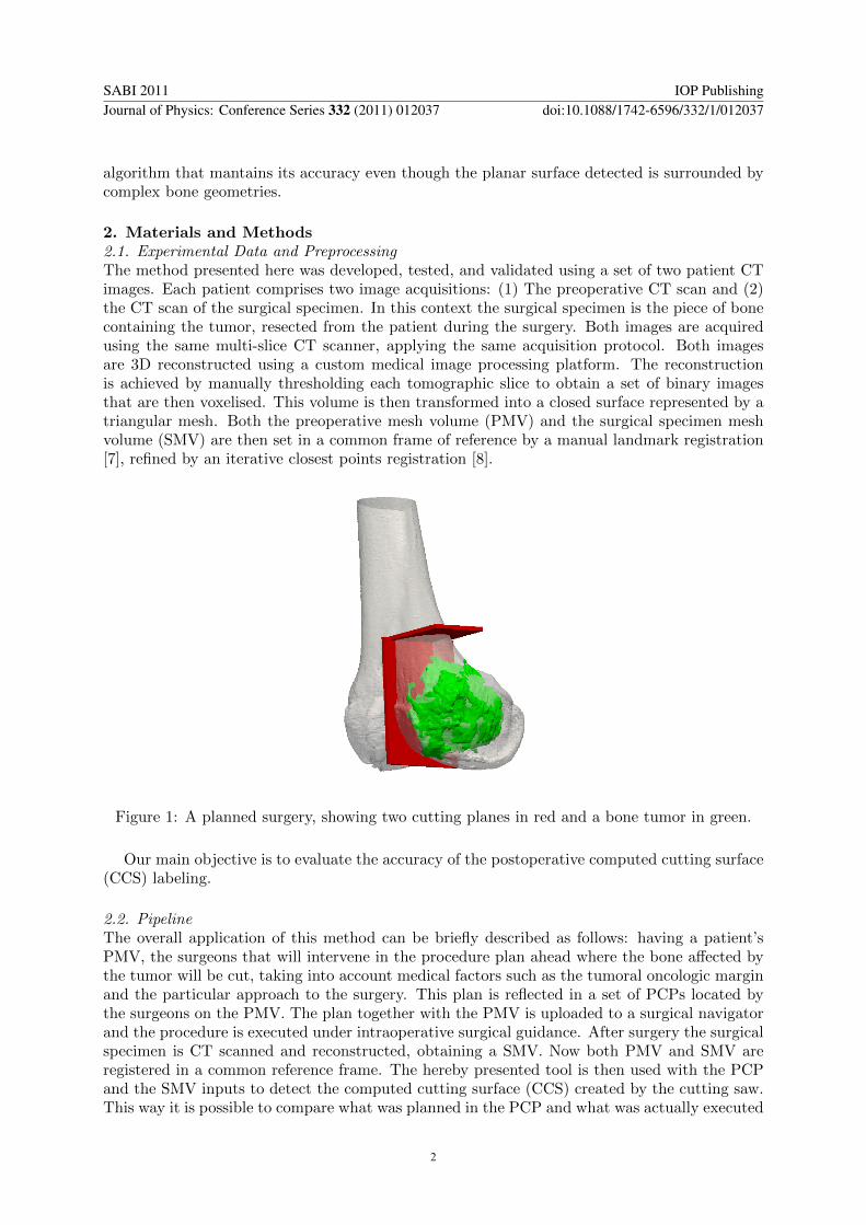
2 Materials and Methods21 Experimental Data and PreprocessingThe method presented here was developed tested and validated using a set of two patient CTimages Each patient comprises two image acquisitions (1) The preoperative CT scan and (2)the CT scan of the surgical specimen In this context the surgical specimen is the piece of bonecontaining the tumor resected from the patient during the surgery Both images are acquiredusing the same multi-slice CT scanner applying the same acquisition protocol Both imagesare 3D reconstructed using a custom medical image processing platform The reconstructionis achieved by manually thresholding each tomographic slice to obtain a set of binary imagesthat are then voxelised This volume is then transformed into a closed surface represented by atriangular mesh Both the preoperative mesh volume (PMV) and the surgical specimen meshvolume (SMV) are then set in a common frame of reference by a manual landmark registration[7] refined by an iterative closest points registration [8]

Figure 1 A planned surgery showing two cutting planes in red and a bone tumor in green

Our main objective is to evaluate the accuracy of the postoperative computed cutting surface(CCS) labeling

22 PipelineThe overall application of this method can be briefly described as follows having a patientrsquosPMV the surgeons that will intervene in the procedure plan ahead where the bone affected bythe tumor will be cut taking into account medical factors such as the tumoral oncologic marginand the particular approach to the surgery This plan is reflected in a set of PCPs located bythe surgeons on the PMV The plan together with the PMV is uploaded to a surgical navigatorand the procedure is executed under intraoperative surgical guidance After surgery the surgicalspecimen is CT scanned and reconstructed obtaining a SMV Now both PMV and SMV areregistered in a common reference frame The hereby presented tool is then used with the PCPand the SMV inputs to detect the computed cutting surface (CCS) created by the cutting sawThis way it is possible to compare what was planned in the PCP and what was actually executed

SABI 2011 IOP PublishingJournal of Physics Conference Series 332 (2011) 012037 doi1010881742-65963321012037

2

in the CCS and measure the errors and discrepancies This work focuses on the algorithm forthe automated labeling of the CCS from the SMV

23 Planar Resection Region Labeling AlgorithmThe algorithm is divided in two phases

(i) Each point of the SMV is projected onto the PCPLet the PCP be described by the plane

ax + by + cz + d = 0

with the normal vector n = (a b c) and x = (x y z)Let SMV be a triangulated 2-manifold representing the surgical specimen We look for theset of points K that belong to the SMV and minimize their normal distance to the PCPFormally

K =

k∣∣∣ku isin SMV and (forallx isin PCP)

(k = argmin

u

|n middot (uminus x)||n|

)(1)

In practice as the SMV is represented by a mesh built on an unstructured grid and it haspotentially infinite points to project the computation is performed in a different way ThePCP is used to generate a 2-dimensional uniform sampling grid applying a homogeneusspacing in both planersquos spanning directions This grid is bounded by the projection of thebounding box of the SMV onto the PCP Each point of the sampling space defined by thisstructured grid is projected onto the SMV in the line along the normal vector of the PCPThe closest point in SMV intersected by the projection of the sampling point is then addedto the point set K that is going to be used in the second part of the algorithm This isdescribed in algorithm 1

Algorithm 1 Projection

Input SMV PCPOutput K a set of points of the SMV that fullfill equation 1

1 UGlarr Generate Uniform Grid from PCP2 K larr empty3 nlarr nnorm(n)4 thresholdlarr 205 for each u in UG do6 min distancelarr Largest Posible Number7 distancelarr 08 while distance lt threshold do9 distancelarr distance + 001

10 k larr u + n middot distance11 if Intersected(k SMV) and distance lt min distance then12 min distancelarr distance13 min k larr k14 end if15 end while16 Add(min kK)17 end for18 return K

SABI 2011 IOP PublishingJournal of Physics Conference Series 332 (2011) 012037 doi1010881742-65963321012037

3

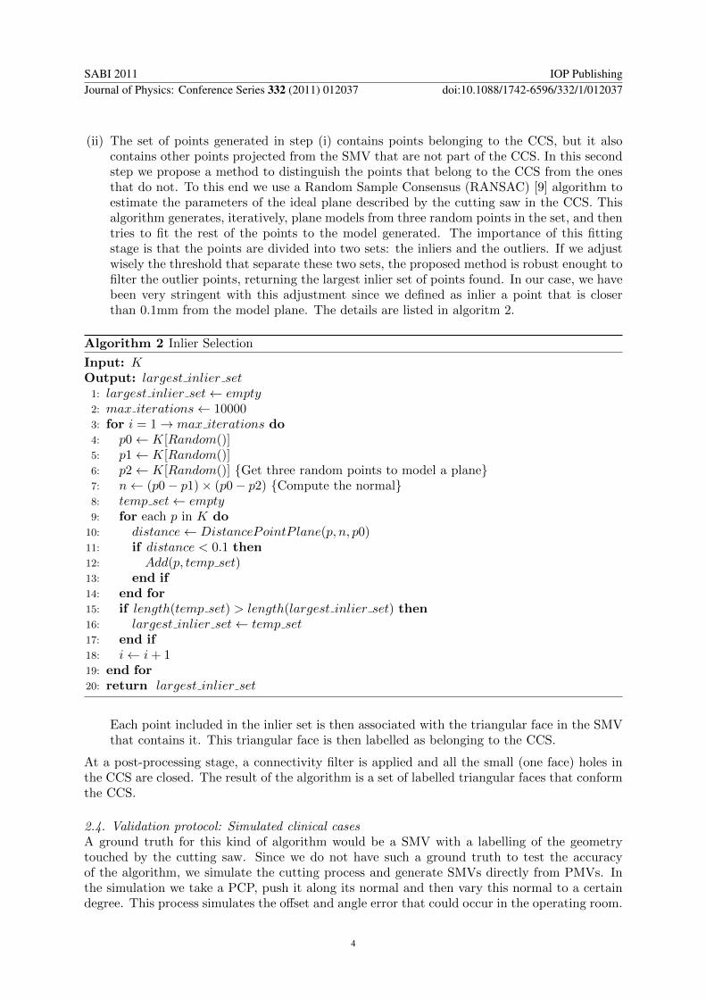
(ii) The set of points generated in step (i) contains points belonging to the CCS but it alsocontains other points projected from the SMV that are not part of the CCS In this secondstep we propose a method to distinguish the points that belong to the CCS from the onesthat do not To this end we use a Random Sample Consensus (RANSAC) [9] algorithm toestimate the parameters of the ideal plane described by the cutting saw in the CCS Thisalgorithm generates iteratively plane models from three random points in the set and thentries to fit the rest of the points to the model generated The importance of this fittingstage is that the points are divided into two sets the inliers and the outliers If we adjustwisely the threshold that separate these two sets the proposed method is robust enought tofilter the outlier points returning the largest inlier set of points found In our case we havebeen very stringent with this adjustment since we defined as inlier a point that is closerthan 01mm from the model plane The details are listed in algoritm 2

Algorithm 2 Inlier Selection

Input KOutput largest inlier set

1 largest inlier setlarr empty2 max iterationslarr 100003 for i = 1rarr max iterations do4 p0larr K[Random()]5 p1larr K[Random()]6 p2larr K[Random()] Get three random points to model a plane7 nlarr (p0minus p1)times (p0minus p2) Compute the normal8 temp setlarr empty9 for each p in K do

10 distancelarr DistancePointP lane(p n p0)11 if distance lt 01 then12 Add(p temp set)13 end if14 end for15 if length(temp set) gt length(largest inlier set) then16 largest inlier setlarr temp set17 end if18 ilarr i + 119 end for20 return largest inlier set

Each point included in the inlier set is then associated with the triangular face in the SMVthat contains it This triangular face is then labelled as belonging to the CCS

At a post-processing stage a connectivity filter is applied and all the small (one face) holes inthe CCS are closed The result of the algorithm is a set of labelled triangular faces that conformthe CCS

24 Validation protocol Simulated clinical casesA ground truth for this kind of algorithm would be a SMV with a labelling of the geometrytouched by the cutting saw Since we do not have such a ground truth to test the accuracyof the algorithm we simulate the cutting process and generate SMVs directly from PMVs Inthe simulation we take a PCP push it along its normal and then vary this normal to a certaindegree This process simulates the offset and angle error that could occur in the operating room

SABI 2011 IOP PublishingJournal of Physics Conference Series 332 (2011) 012037 doi1010881742-65963321012037

4

Figure 2 A simulated resection showing in semitransparent gray the planned cutting plane andin green the simulated cutting plane (distance offset of 2mm and angle of 30)

case distance angle matched not detected not ground truth

1

00 0976 0023 000115 0979 0020 000130 0984 0015 0001

20 0981 0018 000115 0978 0021 000130 0981 0018 0001

50 0982 0017 000015 0981 0019 000130 0981 0016 0003

2

00 0979 0006 001515 0992 0006 000230 0986 0013 0001

20 0994 0005 000115 0988 0011 000130 0993 0007 0000

50 0994 0006 000115 0993 0006 000130 0990 0008 0001

Table 1 Algorithm performance the two cases The distance and angle parameters arecontrolled in the simulation The matched column shows the ratio between the ground trutharea and the detected area that matches with it The not detected column shows the proportionof the area that is in the ground truth but that it was no detected by the algorithm The notground truth column shows the proportion of the area that was detected as being part of thecutting surface but it was not part of the ground truth

Then the PMV is cut generating a SMV and the triangular faces involved in the cut are labelledas belonging to the ground truth Then our algorithm is run with the SMV and the PCP asinputs The resulting CCS is matched to the ground truth following these rules

(i) If a triangular face belongs to the ground truth and to the CCS then the area of that

SABI 2011 IOP PublishingJournal of Physics Conference Series 332 (2011) 012037 doi1010881742-65963321012037

5

(a) Ground truth simulation forcase 1

(b) Detection for case 1

(c) Ground truth simulation forcase 2

(d) Detection for case 2

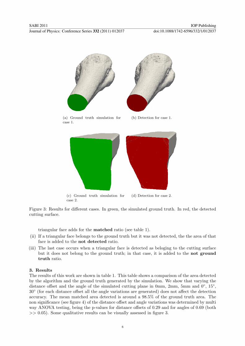
Figure 3 Results for different cases In green the simulated ground truth In red the detectedcutting surface

triangular face adds for the matched ratio (see table 1)

(ii) If a triangular face belongs to the ground truth but it was not detected the the area of thatface is added to the not detected ratio

(iii) The last case occurs when a triangular face is detected as beloging to the cutting surfacebut it does not belong to the ground truth in that case it is added to the not groundtruth ratio

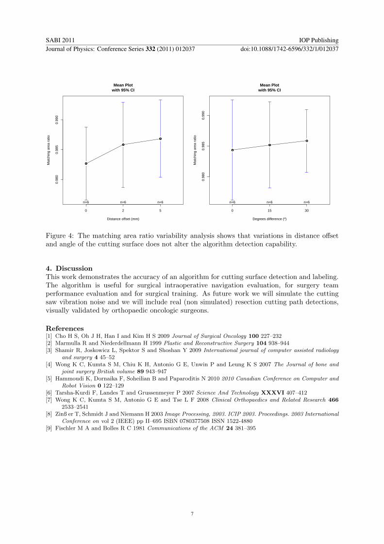
3 ResultsThe results of this work are shown in table 1 This table shows a comparison of the area detectedby the algorithm and the ground truth generated by the simulation We show that varying thedistance offset and the angle of the simulated cutting plane in 0mm 2mm 5mm and 0 1530 (for each distance offset all the angle variations are generated) does not affect the detectionaccuracy The mean matched area detected is around a 985 of the ground truth area Thenon significance (see figure 4) of the distance offset and angle variations was determined by multiway ANOVA testing being the p-values for distance offsets of 029 and for angles of 069 (bothgtgt 005) Some qualitative results can be visually assessed in figure 3

SABI 2011 IOP PublishingJournal of Physics Conference Series 332 (2011) 012037 doi1010881742-65963321012037

6

098

00

985

099

0

Mean Plotwith 95 CI

Distance offset (mm)

Mat

chin

g ar

ea r

atio

0 2 5

n=6 n=6 n=6

098

00

985

099

0

Mean Plotwith 95 CI

Degrees difference (ordm)

Mat

chin

g ar

ea r

atio

0 15 30

n=6 n=6 n=6

Figure 4 The matching area ratio variability analysis shows that variations in distance offsetand angle of the cutting surface does not alter the algorithm detection capability

4 DiscussionThis work demonstrates the accuracy of an algorithm for cutting surface detection and labelingThe algorithm is useful for surgical intraoperative navigation evaluation for surgery teamperformance evaluation and for surgical training As future work we will simulate the cuttingsaw vibration noise and we will include real (non simulated) resection cutting path detectionsvisually validated by orthopaedic oncologic surgeons

References[1] Cho H S Oh J H Han I and Kim H S 2009 Journal of Surgical Oncology 100 227ndash232[2] Marmulla R and Niederdellmann H 1999 Plastic and Reconstructive Surgery 104 938ndash944[3] Shamir R Joskowicz L Spektor S and Shoshan Y 2009 International journal of computer assisted radiology

and surgery 4 45ndash52[4] Wong K C Kumta S M Chiu K H Antonio G E Unwin P and Leung K S 2007 The Journal of bone and

joint surgery British volume 89 943ndash947[5] Hammoudi K Dornaika F Soheilian B and Paparoditis N 2010 2010 Canadian Conference on Computer and

Robot Vision 0 122ndash129[6] Tarsha-Kurdi F Landes T and Grussenmeyer P 2007 Science And Technology XXXVI 407ndash412[7] Wong K C Kumta S M Antonio G E and Tse L F 2008 Clinical Orthopaedics and Related Research 466

2533ndash2541[8] Zinszlig er T Schmidt J and Niemann H 2003 Image Processing 2003 ICIP 2003 Proceedings 2003 International

Conference on vol 2 (IEEE) pp IIndash695 ISBN 0780377508 ISSN 1522-4880[9] Fischler M A and Bolles R C 1981 Communications of the ACM 24 381ndash395

SABI 2011 IOP PublishingJournal of Physics Conference Series 332 (2011) 012037 doi1010881742-65963321012037

7

algorithm that mantains its accuracy even though the planar surface detected is surrounded bycomplex bone geometries

2 Materials and Methods21 Experimental Data and PreprocessingThe method presented here was developed tested and validated using a set of two patient CTimages Each patient comprises two image acquisitions (1) The preoperative CT scan and (2)the CT scan of the surgical specimen In this context the surgical specimen is the piece of bonecontaining the tumor resected from the patient during the surgery Both images are acquiredusing the same multi-slice CT scanner applying the same acquisition protocol Both imagesare 3D reconstructed using a custom medical image processing platform The reconstructionis achieved by manually thresholding each tomographic slice to obtain a set of binary imagesthat are then voxelised This volume is then transformed into a closed surface represented by atriangular mesh Both the preoperative mesh volume (PMV) and the surgical specimen meshvolume (SMV) are then set in a common frame of reference by a manual landmark registration[7] refined by an iterative closest points registration [8]

Figure 1 A planned surgery showing two cutting planes in red and a bone tumor in green

Our main objective is to evaluate the accuracy of the postoperative computed cutting surface(CCS) labeling

22 PipelineThe overall application of this method can be briefly described as follows having a patientrsquosPMV the surgeons that will intervene in the procedure plan ahead where the bone affected bythe tumor will be cut taking into account medical factors such as the tumoral oncologic marginand the particular approach to the surgery This plan is reflected in a set of PCPs located bythe surgeons on the PMV The plan together with the PMV is uploaded to a surgical navigatorand the procedure is executed under intraoperative surgical guidance After surgery the surgicalspecimen is CT scanned and reconstructed obtaining a SMV Now both PMV and SMV areregistered in a common reference frame The hereby presented tool is then used with the PCPand the SMV inputs to detect the computed cutting surface (CCS) created by the cutting sawThis way it is possible to compare what was planned in the PCP and what was actually executed

SABI 2011 IOP PublishingJournal of Physics Conference Series 332 (2011) 012037 doi1010881742-65963321012037

2

in the CCS and measure the errors and discrepancies This work focuses on the algorithm forthe automated labeling of the CCS from the SMV

23 Planar Resection Region Labeling AlgorithmThe algorithm is divided in two phases

(i) Each point of the SMV is projected onto the PCPLet the PCP be described by the plane

ax + by + cz + d = 0

with the normal vector n = (a b c) and x = (x y z)Let SMV be a triangulated 2-manifold representing the surgical specimen We look for theset of points K that belong to the SMV and minimize their normal distance to the PCPFormally

K =

k∣∣∣ku isin SMV and (forallx isin PCP)

(k = argmin

u

|n middot (uminus x)||n|

)(1)

In practice as the SMV is represented by a mesh built on an unstructured grid and it haspotentially infinite points to project the computation is performed in a different way ThePCP is used to generate a 2-dimensional uniform sampling grid applying a homogeneusspacing in both planersquos spanning directions This grid is bounded by the projection of thebounding box of the SMV onto the PCP Each point of the sampling space defined by thisstructured grid is projected onto the SMV in the line along the normal vector of the PCPThe closest point in SMV intersected by the projection of the sampling point is then addedto the point set K that is going to be used in the second part of the algorithm This isdescribed in algorithm 1

Algorithm 1 Projection

Input SMV PCPOutput K a set of points of the SMV that fullfill equation 1

1 UGlarr Generate Uniform Grid from PCP2 K larr empty3 nlarr nnorm(n)4 thresholdlarr 205 for each u in UG do6 min distancelarr Largest Posible Number7 distancelarr 08 while distance lt threshold do9 distancelarr distance + 001

10 k larr u + n middot distance11 if Intersected(k SMV) and distance lt min distance then12 min distancelarr distance13 min k larr k14 end if15 end while16 Add(min kK)17 end for18 return K

SABI 2011 IOP PublishingJournal of Physics Conference Series 332 (2011) 012037 doi1010881742-65963321012037

3

(ii) The set of points generated in step (i) contains points belonging to the CCS but it alsocontains other points projected from the SMV that are not part of the CCS In this secondstep we propose a method to distinguish the points that belong to the CCS from the onesthat do not To this end we use a Random Sample Consensus (RANSAC) [9] algorithm toestimate the parameters of the ideal plane described by the cutting saw in the CCS Thisalgorithm generates iteratively plane models from three random points in the set and thentries to fit the rest of the points to the model generated The importance of this fittingstage is that the points are divided into two sets the inliers and the outliers If we adjustwisely the threshold that separate these two sets the proposed method is robust enought tofilter the outlier points returning the largest inlier set of points found In our case we havebeen very stringent with this adjustment since we defined as inlier a point that is closerthan 01mm from the model plane The details are listed in algoritm 2

Algorithm 2 Inlier Selection

Input KOutput largest inlier set

1 largest inlier setlarr empty2 max iterationslarr 100003 for i = 1rarr max iterations do4 p0larr K[Random()]5 p1larr K[Random()]6 p2larr K[Random()] Get three random points to model a plane7 nlarr (p0minus p1)times (p0minus p2) Compute the normal8 temp setlarr empty9 for each p in K do

10 distancelarr DistancePointP lane(p n p0)11 if distance lt 01 then12 Add(p temp set)13 end if14 end for15 if length(temp set) gt length(largest inlier set) then16 largest inlier setlarr temp set17 end if18 ilarr i + 119 end for20 return largest inlier set

Each point included in the inlier set is then associated with the triangular face in the SMVthat contains it This triangular face is then labelled as belonging to the CCS

At a post-processing stage a connectivity filter is applied and all the small (one face) holes inthe CCS are closed The result of the algorithm is a set of labelled triangular faces that conformthe CCS

24 Validation protocol Simulated clinical casesA ground truth for this kind of algorithm would be a SMV with a labelling of the geometrytouched by the cutting saw Since we do not have such a ground truth to test the accuracyof the algorithm we simulate the cutting process and generate SMVs directly from PMVs Inthe simulation we take a PCP push it along its normal and then vary this normal to a certaindegree This process simulates the offset and angle error that could occur in the operating room

SABI 2011 IOP PublishingJournal of Physics Conference Series 332 (2011) 012037 doi1010881742-65963321012037

4

Figure 2 A simulated resection showing in semitransparent gray the planned cutting plane andin green the simulated cutting plane (distance offset of 2mm and angle of 30)

case distance angle matched not detected not ground truth

1

00 0976 0023 000115 0979 0020 000130 0984 0015 0001

20 0981 0018 000115 0978 0021 000130 0981 0018 0001

50 0982 0017 000015 0981 0019 000130 0981 0016 0003

2

00 0979 0006 001515 0992 0006 000230 0986 0013 0001

20 0994 0005 000115 0988 0011 000130 0993 0007 0000

50 0994 0006 000115 0993 0006 000130 0990 0008 0001

Table 1 Algorithm performance the two cases The distance and angle parameters arecontrolled in the simulation The matched column shows the ratio between the ground trutharea and the detected area that matches with it The not detected column shows the proportionof the area that is in the ground truth but that it was no detected by the algorithm The notground truth column shows the proportion of the area that was detected as being part of thecutting surface but it was not part of the ground truth

Then the PMV is cut generating a SMV and the triangular faces involved in the cut are labelledas belonging to the ground truth Then our algorithm is run with the SMV and the PCP asinputs The resulting CCS is matched to the ground truth following these rules

(i) If a triangular face belongs to the ground truth and to the CCS then the area of that

SABI 2011 IOP PublishingJournal of Physics Conference Series 332 (2011) 012037 doi1010881742-65963321012037

5

(a) Ground truth simulation forcase 1

(b) Detection for case 1

(c) Ground truth simulation forcase 2

(d) Detection for case 2

Figure 3 Results for different cases In green the simulated ground truth In red the detectedcutting surface

triangular face adds for the matched ratio (see table 1)

(ii) If a triangular face belongs to the ground truth but it was not detected the the area of thatface is added to the not detected ratio

(iii) The last case occurs when a triangular face is detected as beloging to the cutting surfacebut it does not belong to the ground truth in that case it is added to the not groundtruth ratio

3 ResultsThe results of this work are shown in table 1 This table shows a comparison of the area detectedby the algorithm and the ground truth generated by the simulation We show that varying thedistance offset and the angle of the simulated cutting plane in 0mm 2mm 5mm and 0 1530 (for each distance offset all the angle variations are generated) does not affect the detectionaccuracy The mean matched area detected is around a 985 of the ground truth area Thenon significance (see figure 4) of the distance offset and angle variations was determined by multiway ANOVA testing being the p-values for distance offsets of 029 and for angles of 069 (bothgtgt 005) Some qualitative results can be visually assessed in figure 3

SABI 2011 IOP PublishingJournal of Physics Conference Series 332 (2011) 012037 doi1010881742-65963321012037

6

098

00

985

099

0

Mean Plotwith 95 CI

Distance offset (mm)

Mat

chin

g ar

ea r

atio

0 2 5

n=6 n=6 n=6

098

00

985

099

0

Mean Plotwith 95 CI

Degrees difference (ordm)

Mat

chin

g ar

ea r

atio

0 15 30

n=6 n=6 n=6

Figure 4 The matching area ratio variability analysis shows that variations in distance offsetand angle of the cutting surface does not alter the algorithm detection capability

4 DiscussionThis work demonstrates the accuracy of an algorithm for cutting surface detection and labelingThe algorithm is useful for surgical intraoperative navigation evaluation for surgery teamperformance evaluation and for surgical training As future work we will simulate the cuttingsaw vibration noise and we will include real (non simulated) resection cutting path detectionsvisually validated by orthopaedic oncologic surgeons

References[1] Cho H S Oh J H Han I and Kim H S 2009 Journal of Surgical Oncology 100 227ndash232[2] Marmulla R and Niederdellmann H 1999 Plastic and Reconstructive Surgery 104 938ndash944[3] Shamir R Joskowicz L Spektor S and Shoshan Y 2009 International journal of computer assisted radiology

and surgery 4 45ndash52[4] Wong K C Kumta S M Chiu K H Antonio G E Unwin P and Leung K S 2007 The Journal of bone and

joint surgery British volume 89 943ndash947[5] Hammoudi K Dornaika F Soheilian B and Paparoditis N 2010 2010 Canadian Conference on Computer and

Robot Vision 0 122ndash129[6] Tarsha-Kurdi F Landes T and Grussenmeyer P 2007 Science And Technology XXXVI 407ndash412[7] Wong K C Kumta S M Antonio G E and Tse L F 2008 Clinical Orthopaedics and Related Research 466

2533ndash2541[8] Zinszlig er T Schmidt J and Niemann H 2003 Image Processing 2003 ICIP 2003 Proceedings 2003 International

Conference on vol 2 (IEEE) pp IIndash695 ISBN 0780377508 ISSN 1522-4880[9] Fischler M A and Bolles R C 1981 Communications of the ACM 24 381ndash395

SABI 2011 IOP PublishingJournal of Physics Conference Series 332 (2011) 012037 doi1010881742-65963321012037

7

in the CCS and measure the errors and discrepancies This work focuses on the algorithm forthe automated labeling of the CCS from the SMV

23 Planar Resection Region Labeling AlgorithmThe algorithm is divided in two phases

(i) Each point of the SMV is projected onto the PCPLet the PCP be described by the plane

ax + by + cz + d = 0

with the normal vector n = (a b c) and x = (x y z)Let SMV be a triangulated 2-manifold representing the surgical specimen We look for theset of points K that belong to the SMV and minimize their normal distance to the PCPFormally

K =

k∣∣∣ku isin SMV and (forallx isin PCP)

(k = argmin

u

|n middot (uminus x)||n|

)(1)

In practice as the SMV is represented by a mesh built on an unstructured grid and it haspotentially infinite points to project the computation is performed in a different way ThePCP is used to generate a 2-dimensional uniform sampling grid applying a homogeneusspacing in both planersquos spanning directions This grid is bounded by the projection of thebounding box of the SMV onto the PCP Each point of the sampling space defined by thisstructured grid is projected onto the SMV in the line along the normal vector of the PCPThe closest point in SMV intersected by the projection of the sampling point is then addedto the point set K that is going to be used in the second part of the algorithm This isdescribed in algorithm 1

Algorithm 1 Projection

Input SMV PCPOutput K a set of points of the SMV that fullfill equation 1

1 UGlarr Generate Uniform Grid from PCP2 K larr empty3 nlarr nnorm(n)4 thresholdlarr 205 for each u in UG do6 min distancelarr Largest Posible Number7 distancelarr 08 while distance lt threshold do9 distancelarr distance + 001

10 k larr u + n middot distance11 if Intersected(k SMV) and distance lt min distance then12 min distancelarr distance13 min k larr k14 end if15 end while16 Add(min kK)17 end for18 return K

SABI 2011 IOP PublishingJournal of Physics Conference Series 332 (2011) 012037 doi1010881742-65963321012037

3

(ii) The set of points generated in step (i) contains points belonging to the CCS but it alsocontains other points projected from the SMV that are not part of the CCS In this secondstep we propose a method to distinguish the points that belong to the CCS from the onesthat do not To this end we use a Random Sample Consensus (RANSAC) [9] algorithm toestimate the parameters of the ideal plane described by the cutting saw in the CCS Thisalgorithm generates iteratively plane models from three random points in the set and thentries to fit the rest of the points to the model generated The importance of this fittingstage is that the points are divided into two sets the inliers and the outliers If we adjustwisely the threshold that separate these two sets the proposed method is robust enought tofilter the outlier points returning the largest inlier set of points found In our case we havebeen very stringent with this adjustment since we defined as inlier a point that is closerthan 01mm from the model plane The details are listed in algoritm 2

Algorithm 2 Inlier Selection

Input KOutput largest inlier set

1 largest inlier setlarr empty2 max iterationslarr 100003 for i = 1rarr max iterations do4 p0larr K[Random()]5 p1larr K[Random()]6 p2larr K[Random()] Get three random points to model a plane7 nlarr (p0minus p1)times (p0minus p2) Compute the normal8 temp setlarr empty9 for each p in K do

10 distancelarr DistancePointP lane(p n p0)11 if distance lt 01 then12 Add(p temp set)13 end if14 end for15 if length(temp set) gt length(largest inlier set) then16 largest inlier setlarr temp set17 end if18 ilarr i + 119 end for20 return largest inlier set

Each point included in the inlier set is then associated with the triangular face in the SMVthat contains it This triangular face is then labelled as belonging to the CCS

At a post-processing stage a connectivity filter is applied and all the small (one face) holes inthe CCS are closed The result of the algorithm is a set of labelled triangular faces that conformthe CCS

24 Validation protocol Simulated clinical casesA ground truth for this kind of algorithm would be a SMV with a labelling of the geometrytouched by the cutting saw Since we do not have such a ground truth to test the accuracyof the algorithm we simulate the cutting process and generate SMVs directly from PMVs Inthe simulation we take a PCP push it along its normal and then vary this normal to a certaindegree This process simulates the offset and angle error that could occur in the operating room

SABI 2011 IOP PublishingJournal of Physics Conference Series 332 (2011) 012037 doi1010881742-65963321012037

4

Figure 2 A simulated resection showing in semitransparent gray the planned cutting plane andin green the simulated cutting plane (distance offset of 2mm and angle of 30)

case distance angle matched not detected not ground truth

1

00 0976 0023 000115 0979 0020 000130 0984 0015 0001

20 0981 0018 000115 0978 0021 000130 0981 0018 0001

50 0982 0017 000015 0981 0019 000130 0981 0016 0003

2

00 0979 0006 001515 0992 0006 000230 0986 0013 0001

20 0994 0005 000115 0988 0011 000130 0993 0007 0000

50 0994 0006 000115 0993 0006 000130 0990 0008 0001

Table 1 Algorithm performance the two cases The distance and angle parameters arecontrolled in the simulation The matched column shows the ratio between the ground trutharea and the detected area that matches with it The not detected column shows the proportionof the area that is in the ground truth but that it was no detected by the algorithm The notground truth column shows the proportion of the area that was detected as being part of thecutting surface but it was not part of the ground truth

Then the PMV is cut generating a SMV and the triangular faces involved in the cut are labelledas belonging to the ground truth Then our algorithm is run with the SMV and the PCP asinputs The resulting CCS is matched to the ground truth following these rules

(i) If a triangular face belongs to the ground truth and to the CCS then the area of that

SABI 2011 IOP PublishingJournal of Physics Conference Series 332 (2011) 012037 doi1010881742-65963321012037

5

(a) Ground truth simulation forcase 1

(b) Detection for case 1

(c) Ground truth simulation forcase 2

(d) Detection for case 2

Figure 3 Results for different cases In green the simulated ground truth In red the detectedcutting surface

triangular face adds for the matched ratio (see table 1)

(ii) If a triangular face belongs to the ground truth but it was not detected the the area of thatface is added to the not detected ratio

(iii) The last case occurs when a triangular face is detected as beloging to the cutting surfacebut it does not belong to the ground truth in that case it is added to the not groundtruth ratio

3 ResultsThe results of this work are shown in table 1 This table shows a comparison of the area detectedby the algorithm and the ground truth generated by the simulation We show that varying thedistance offset and the angle of the simulated cutting plane in 0mm 2mm 5mm and 0 1530 (for each distance offset all the angle variations are generated) does not affect the detectionaccuracy The mean matched area detected is around a 985 of the ground truth area Thenon significance (see figure 4) of the distance offset and angle variations was determined by multiway ANOVA testing being the p-values for distance offsets of 029 and for angles of 069 (bothgtgt 005) Some qualitative results can be visually assessed in figure 3

SABI 2011 IOP PublishingJournal of Physics Conference Series 332 (2011) 012037 doi1010881742-65963321012037

6

098

00

985

099

0

Mean Plotwith 95 CI

Distance offset (mm)

Mat

chin

g ar

ea r

atio

0 2 5

n=6 n=6 n=6

098

00

985

099

0

Mean Plotwith 95 CI

Degrees difference (ordm)

Mat

chin

g ar

ea r

atio

0 15 30

n=6 n=6 n=6

Figure 4 The matching area ratio variability analysis shows that variations in distance offsetand angle of the cutting surface does not alter the algorithm detection capability

4 DiscussionThis work demonstrates the accuracy of an algorithm for cutting surface detection and labelingThe algorithm is useful for surgical intraoperative navigation evaluation for surgery teamperformance evaluation and for surgical training As future work we will simulate the cuttingsaw vibration noise and we will include real (non simulated) resection cutting path detectionsvisually validated by orthopaedic oncologic surgeons

References[1] Cho H S Oh J H Han I and Kim H S 2009 Journal of Surgical Oncology 100 227ndash232[2] Marmulla R and Niederdellmann H 1999 Plastic and Reconstructive Surgery 104 938ndash944[3] Shamir R Joskowicz L Spektor S and Shoshan Y 2009 International journal of computer assisted radiology

and surgery 4 45ndash52[4] Wong K C Kumta S M Chiu K H Antonio G E Unwin P and Leung K S 2007 The Journal of bone and

joint surgery British volume 89 943ndash947[5] Hammoudi K Dornaika F Soheilian B and Paparoditis N 2010 2010 Canadian Conference on Computer and

Robot Vision 0 122ndash129[6] Tarsha-Kurdi F Landes T and Grussenmeyer P 2007 Science And Technology XXXVI 407ndash412[7] Wong K C Kumta S M Antonio G E and Tse L F 2008 Clinical Orthopaedics and Related Research 466

2533ndash2541[8] Zinszlig er T Schmidt J and Niemann H 2003 Image Processing 2003 ICIP 2003 Proceedings 2003 International

Conference on vol 2 (IEEE) pp IIndash695 ISBN 0780377508 ISSN 1522-4880[9] Fischler M A and Bolles R C 1981 Communications of the ACM 24 381ndash395

SABI 2011 IOP PublishingJournal of Physics Conference Series 332 (2011) 012037 doi1010881742-65963321012037

7

(ii) The set of points generated in step (i) contains points belonging to the CCS but it alsocontains other points projected from the SMV that are not part of the CCS In this secondstep we propose a method to distinguish the points that belong to the CCS from the onesthat do not To this end we use a Random Sample Consensus (RANSAC) [9] algorithm toestimate the parameters of the ideal plane described by the cutting saw in the CCS Thisalgorithm generates iteratively plane models from three random points in the set and thentries to fit the rest of the points to the model generated The importance of this fittingstage is that the points are divided into two sets the inliers and the outliers If we adjustwisely the threshold that separate these two sets the proposed method is robust enought tofilter the outlier points returning the largest inlier set of points found In our case we havebeen very stringent with this adjustment since we defined as inlier a point that is closerthan 01mm from the model plane The details are listed in algoritm 2

Algorithm 2 Inlier Selection

Input KOutput largest inlier set

1 largest inlier setlarr empty2 max iterationslarr 100003 for i = 1rarr max iterations do4 p0larr K[Random()]5 p1larr K[Random()]6 p2larr K[Random()] Get three random points to model a plane7 nlarr (p0minus p1)times (p0minus p2) Compute the normal8 temp setlarr empty9 for each p in K do

10 distancelarr DistancePointP lane(p n p0)11 if distance lt 01 then12 Add(p temp set)13 end if14 end for15 if length(temp set) gt length(largest inlier set) then16 largest inlier setlarr temp set17 end if18 ilarr i + 119 end for20 return largest inlier set

Each point included in the inlier set is then associated with the triangular face in the SMVthat contains it This triangular face is then labelled as belonging to the CCS

At a post-processing stage a connectivity filter is applied and all the small (one face) holes inthe CCS are closed The result of the algorithm is a set of labelled triangular faces that conformthe CCS

24 Validation protocol Simulated clinical casesA ground truth for this kind of algorithm would be a SMV with a labelling of the geometrytouched by the cutting saw Since we do not have such a ground truth to test the accuracyof the algorithm we simulate the cutting process and generate SMVs directly from PMVs Inthe simulation we take a PCP push it along its normal and then vary this normal to a certaindegree This process simulates the offset and angle error that could occur in the operating room

SABI 2011 IOP PublishingJournal of Physics Conference Series 332 (2011) 012037 doi1010881742-65963321012037

4

Figure 2 A simulated resection showing in semitransparent gray the planned cutting plane andin green the simulated cutting plane (distance offset of 2mm and angle of 30)

case distance angle matched not detected not ground truth

1

00 0976 0023 000115 0979 0020 000130 0984 0015 0001

20 0981 0018 000115 0978 0021 000130 0981 0018 0001

50 0982 0017 000015 0981 0019 000130 0981 0016 0003

2

00 0979 0006 001515 0992 0006 000230 0986 0013 0001

20 0994 0005 000115 0988 0011 000130 0993 0007 0000

50 0994 0006 000115 0993 0006 000130 0990 0008 0001

Table 1 Algorithm performance the two cases The distance and angle parameters arecontrolled in the simulation The matched column shows the ratio between the ground trutharea and the detected area that matches with it The not detected column shows the proportionof the area that is in the ground truth but that it was no detected by the algorithm The notground truth column shows the proportion of the area that was detected as being part of thecutting surface but it was not part of the ground truth

Then the PMV is cut generating a SMV and the triangular faces involved in the cut are labelledas belonging to the ground truth Then our algorithm is run with the SMV and the PCP asinputs The resulting CCS is matched to the ground truth following these rules

(i) If a triangular face belongs to the ground truth and to the CCS then the area of that

SABI 2011 IOP PublishingJournal of Physics Conference Series 332 (2011) 012037 doi1010881742-65963321012037

5

(a) Ground truth simulation forcase 1

(b) Detection for case 1

(c) Ground truth simulation forcase 2

(d) Detection for case 2

Figure 3 Results for different cases In green the simulated ground truth In red the detectedcutting surface

triangular face adds for the matched ratio (see table 1)

(ii) If a triangular face belongs to the ground truth but it was not detected the the area of thatface is added to the not detected ratio

(iii) The last case occurs when a triangular face is detected as beloging to the cutting surfacebut it does not belong to the ground truth in that case it is added to the not groundtruth ratio

3 ResultsThe results of this work are shown in table 1 This table shows a comparison of the area detectedby the algorithm and the ground truth generated by the simulation We show that varying thedistance offset and the angle of the simulated cutting plane in 0mm 2mm 5mm and 0 1530 (for each distance offset all the angle variations are generated) does not affect the detectionaccuracy The mean matched area detected is around a 985 of the ground truth area Thenon significance (see figure 4) of the distance offset and angle variations was determined by multiway ANOVA testing being the p-values for distance offsets of 029 and for angles of 069 (bothgtgt 005) Some qualitative results can be visually assessed in figure 3

SABI 2011 IOP PublishingJournal of Physics Conference Series 332 (2011) 012037 doi1010881742-65963321012037

6

098

00

985

099

0

Mean Plotwith 95 CI

Distance offset (mm)

Mat

chin

g ar

ea r

atio

0 2 5

n=6 n=6 n=6

098

00

985

099

0

Mean Plotwith 95 CI

Degrees difference (ordm)

Mat

chin

g ar

ea r

atio

0 15 30

n=6 n=6 n=6

Figure 4 The matching area ratio variability analysis shows that variations in distance offsetand angle of the cutting surface does not alter the algorithm detection capability

4 DiscussionThis work demonstrates the accuracy of an algorithm for cutting surface detection and labelingThe algorithm is useful for surgical intraoperative navigation evaluation for surgery teamperformance evaluation and for surgical training As future work we will simulate the cuttingsaw vibration noise and we will include real (non simulated) resection cutting path detectionsvisually validated by orthopaedic oncologic surgeons

References[1] Cho H S Oh J H Han I and Kim H S 2009 Journal of Surgical Oncology 100 227ndash232[2] Marmulla R and Niederdellmann H 1999 Plastic and Reconstructive Surgery 104 938ndash944[3] Shamir R Joskowicz L Spektor S and Shoshan Y 2009 International journal of computer assisted radiology

and surgery 4 45ndash52[4] Wong K C Kumta S M Chiu K H Antonio G E Unwin P and Leung K S 2007 The Journal of bone and

joint surgery British volume 89 943ndash947[5] Hammoudi K Dornaika F Soheilian B and Paparoditis N 2010 2010 Canadian Conference on Computer and

Robot Vision 0 122ndash129[6] Tarsha-Kurdi F Landes T and Grussenmeyer P 2007 Science And Technology XXXVI 407ndash412[7] Wong K C Kumta S M Antonio G E and Tse L F 2008 Clinical Orthopaedics and Related Research 466

2533ndash2541[8] Zinszlig er T Schmidt J and Niemann H 2003 Image Processing 2003 ICIP 2003 Proceedings 2003 International

Conference on vol 2 (IEEE) pp IIndash695 ISBN 0780377508 ISSN 1522-4880[9] Fischler M A and Bolles R C 1981 Communications of the ACM 24 381ndash395

SABI 2011 IOP PublishingJournal of Physics Conference Series 332 (2011) 012037 doi1010881742-65963321012037

7

Figure 2 A simulated resection showing in semitransparent gray the planned cutting plane andin green the simulated cutting plane (distance offset of 2mm and angle of 30)

case distance angle matched not detected not ground truth

1

00 0976 0023 000115 0979 0020 000130 0984 0015 0001

20 0981 0018 000115 0978 0021 000130 0981 0018 0001

50 0982 0017 000015 0981 0019 000130 0981 0016 0003

2

00 0979 0006 001515 0992 0006 000230 0986 0013 0001

20 0994 0005 000115 0988 0011 000130 0993 0007 0000

50 0994 0006 000115 0993 0006 000130 0990 0008 0001

Table 1 Algorithm performance the two cases The distance and angle parameters arecontrolled in the simulation The matched column shows the ratio between the ground trutharea and the detected area that matches with it The not detected column shows the proportionof the area that is in the ground truth but that it was no detected by the algorithm The notground truth column shows the proportion of the area that was detected as being part of thecutting surface but it was not part of the ground truth

Then the PMV is cut generating a SMV and the triangular faces involved in the cut are labelledas belonging to the ground truth Then our algorithm is run with the SMV and the PCP asinputs The resulting CCS is matched to the ground truth following these rules

(i) If a triangular face belongs to the ground truth and to the CCS then the area of that

SABI 2011 IOP PublishingJournal of Physics Conference Series 332 (2011) 012037 doi1010881742-65963321012037

5

(a) Ground truth simulation forcase 1

(b) Detection for case 1

(c) Ground truth simulation forcase 2

(d) Detection for case 2

Figure 3 Results for different cases In green the simulated ground truth In red the detectedcutting surface

triangular face adds for the matched ratio (see table 1)

(ii) If a triangular face belongs to the ground truth but it was not detected the the area of thatface is added to the not detected ratio

(iii) The last case occurs when a triangular face is detected as beloging to the cutting surfacebut it does not belong to the ground truth in that case it is added to the not groundtruth ratio

3 ResultsThe results of this work are shown in table 1 This table shows a comparison of the area detectedby the algorithm and the ground truth generated by the simulation We show that varying thedistance offset and the angle of the simulated cutting plane in 0mm 2mm 5mm and 0 1530 (for each distance offset all the angle variations are generated) does not affect the detectionaccuracy The mean matched area detected is around a 985 of the ground truth area Thenon significance (see figure 4) of the distance offset and angle variations was determined by multiway ANOVA testing being the p-values for distance offsets of 029 and for angles of 069 (bothgtgt 005) Some qualitative results can be visually assessed in figure 3

SABI 2011 IOP PublishingJournal of Physics Conference Series 332 (2011) 012037 doi1010881742-65963321012037

6

098

00

985

099

0

Mean Plotwith 95 CI

Distance offset (mm)

Mat

chin

g ar

ea r

atio

0 2 5

n=6 n=6 n=6

098

00

985

099

0

Mean Plotwith 95 CI

Degrees difference (ordm)

Mat

chin

g ar

ea r

atio

0 15 30

n=6 n=6 n=6

Figure 4 The matching area ratio variability analysis shows that variations in distance offsetand angle of the cutting surface does not alter the algorithm detection capability

4 DiscussionThis work demonstrates the accuracy of an algorithm for cutting surface detection and labelingThe algorithm is useful for surgical intraoperative navigation evaluation for surgery teamperformance evaluation and for surgical training As future work we will simulate the cuttingsaw vibration noise and we will include real (non simulated) resection cutting path detectionsvisually validated by orthopaedic oncologic surgeons

References[1] Cho H S Oh J H Han I and Kim H S 2009 Journal of Surgical Oncology 100 227ndash232[2] Marmulla R and Niederdellmann H 1999 Plastic and Reconstructive Surgery 104 938ndash944[3] Shamir R Joskowicz L Spektor S and Shoshan Y 2009 International journal of computer assisted radiology

and surgery 4 45ndash52[4] Wong K C Kumta S M Chiu K H Antonio G E Unwin P and Leung K S 2007 The Journal of bone and

joint surgery British volume 89 943ndash947[5] Hammoudi K Dornaika F Soheilian B and Paparoditis N 2010 2010 Canadian Conference on Computer and

Robot Vision 0 122ndash129[6] Tarsha-Kurdi F Landes T and Grussenmeyer P 2007 Science And Technology XXXVI 407ndash412[7] Wong K C Kumta S M Antonio G E and Tse L F 2008 Clinical Orthopaedics and Related Research 466

2533ndash2541[8] Zinszlig er T Schmidt J and Niemann H 2003 Image Processing 2003 ICIP 2003 Proceedings 2003 International

Conference on vol 2 (IEEE) pp IIndash695 ISBN 0780377508 ISSN 1522-4880[9] Fischler M A and Bolles R C 1981 Communications of the ACM 24 381ndash395

SABI 2011 IOP PublishingJournal of Physics Conference Series 332 (2011) 012037 doi1010881742-65963321012037

7

(a) Ground truth simulation forcase 1

(b) Detection for case 1

(c) Ground truth simulation forcase 2

(d) Detection for case 2

Figure 3 Results for different cases In green the simulated ground truth In red the detectedcutting surface

triangular face adds for the matched ratio (see table 1)

(ii) If a triangular face belongs to the ground truth but it was not detected the the area of thatface is added to the not detected ratio

(iii) The last case occurs when a triangular face is detected as beloging to the cutting surfacebut it does not belong to the ground truth in that case it is added to the not groundtruth ratio

3 ResultsThe results of this work are shown in table 1 This table shows a comparison of the area detectedby the algorithm and the ground truth generated by the simulation We show that varying thedistance offset and the angle of the simulated cutting plane in 0mm 2mm 5mm and 0 1530 (for each distance offset all the angle variations are generated) does not affect the detectionaccuracy The mean matched area detected is around a 985 of the ground truth area Thenon significance (see figure 4) of the distance offset and angle variations was determined by multiway ANOVA testing being the p-values for distance offsets of 029 and for angles of 069 (bothgtgt 005) Some qualitative results can be visually assessed in figure 3

SABI 2011 IOP PublishingJournal of Physics Conference Series 332 (2011) 012037 doi1010881742-65963321012037

6

098

00

985

099

0

Mean Plotwith 95 CI

Distance offset (mm)

Mat

chin

g ar

ea r

atio

0 2 5

n=6 n=6 n=6

098

00

985

099

0

Mean Plotwith 95 CI

Degrees difference (ordm)

Mat

chin

g ar

ea r

atio

0 15 30

n=6 n=6 n=6

Figure 4 The matching area ratio variability analysis shows that variations in distance offsetand angle of the cutting surface does not alter the algorithm detection capability

4 DiscussionThis work demonstrates the accuracy of an algorithm for cutting surface detection and labelingThe algorithm is useful for surgical intraoperative navigation evaluation for surgery teamperformance evaluation and for surgical training As future work we will simulate the cuttingsaw vibration noise and we will include real (non simulated) resection cutting path detectionsvisually validated by orthopaedic oncologic surgeons

References[1] Cho H S Oh J H Han I and Kim H S 2009 Journal of Surgical Oncology 100 227ndash232[2] Marmulla R and Niederdellmann H 1999 Plastic and Reconstructive Surgery 104 938ndash944[3] Shamir R Joskowicz L Spektor S and Shoshan Y 2009 International journal of computer assisted radiology

and surgery 4 45ndash52[4] Wong K C Kumta S M Chiu K H Antonio G E Unwin P and Leung K S 2007 The Journal of bone and

joint surgery British volume 89 943ndash947[5] Hammoudi K Dornaika F Soheilian B and Paparoditis N 2010 2010 Canadian Conference on Computer and

Robot Vision 0 122ndash129[6] Tarsha-Kurdi F Landes T and Grussenmeyer P 2007 Science And Technology XXXVI 407ndash412[7] Wong K C Kumta S M Antonio G E and Tse L F 2008 Clinical Orthopaedics and Related Research 466

2533ndash2541[8] Zinszlig er T Schmidt J and Niemann H 2003 Image Processing 2003 ICIP 2003 Proceedings 2003 International

Conference on vol 2 (IEEE) pp IIndash695 ISBN 0780377508 ISSN 1522-4880[9] Fischler M A and Bolles R C 1981 Communications of the ACM 24 381ndash395

SABI 2011 IOP PublishingJournal of Physics Conference Series 332 (2011) 012037 doi1010881742-65963321012037

7

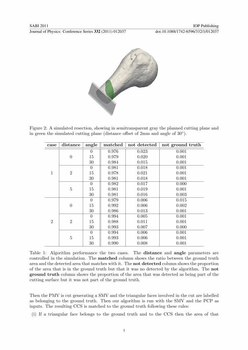
098

00

985

099

0

Mean Plotwith 95 CI

Distance offset (mm)

Mat

chin

g ar

ea r

atio

0 2 5

n=6 n=6 n=6

098

00

985

099

0

Mean Plotwith 95 CI

Degrees difference (ordm)

Mat

chin

g ar

ea r

atio

0 15 30

n=6 n=6 n=6

Figure 4 The matching area ratio variability analysis shows that variations in distance offsetand angle of the cutting surface does not alter the algorithm detection capability

4 DiscussionThis work demonstrates the accuracy of an algorithm for cutting surface detection and labelingThe algorithm is useful for surgical intraoperative navigation evaluation for surgery teamperformance evaluation and for surgical training As future work we will simulate the cuttingsaw vibration noise and we will include real (non simulated) resection cutting path detectionsvisually validated by orthopaedic oncologic surgeons

References[1] Cho H S Oh J H Han I and Kim H S 2009 Journal of Surgical Oncology 100 227ndash232[2] Marmulla R and Niederdellmann H 1999 Plastic and Reconstructive Surgery 104 938ndash944[3] Shamir R Joskowicz L Spektor S and Shoshan Y 2009 International journal of computer assisted radiology

and surgery 4 45ndash52[4] Wong K C Kumta S M Chiu K H Antonio G E Unwin P and Leung K S 2007 The Journal of bone and

joint surgery British volume 89 943ndash947[5] Hammoudi K Dornaika F Soheilian B and Paparoditis N 2010 2010 Canadian Conference on Computer and

Robot Vision 0 122ndash129[6] Tarsha-Kurdi F Landes T and Grussenmeyer P 2007 Science And Technology XXXVI 407ndash412[7] Wong K C Kumta S M Antonio G E and Tse L F 2008 Clinical Orthopaedics and Related Research 466

2533ndash2541[8] Zinszlig er T Schmidt J and Niemann H 2003 Image Processing 2003 ICIP 2003 Proceedings 2003 International

Conference on vol 2 (IEEE) pp IIndash695 ISBN 0780377508 ISSN 1522-4880[9] Fischler M A and Bolles R C 1981 Communications of the ACM 24 381ndash395

SABI 2011 IOP PublishingJournal of Physics Conference Series 332 (2011) 012037 doi1010881742-65963321012037

7