AN ALGORITHM FOR COMPUTING THE UNION, INTERSECTION OR ...jarek/graphics/papers/04PolygonBooleansMargali… · AN ALGORITHM FOR COMPUTING THE UNION, INTERSECTION OR DIFFERENCE

Comput & Graphics VoI. 13, No 2, pp 167-183, 1989 Printed in Great Britain

0091-8493/89 $3.00 + .00 © 1989 Maxwell Pergamon Macmillan plc

Technical Section

AN ALGORITHM FOR COMPUTING THE UNION, INTERSECTION OR DIFFERENCE OF TWO POLYGONS

AVRAHAM MARGALIT Computer Vision Laboratory, Center for Automation Research, University of Maryland,

College Park, MD 20742

and

GARY D. KNOTT Department of Computer Science, University of Maryland, College Park, MD 20742

Abstract-An algorithm for set operations on pairs of polygons is presented. The algorithm uses a boundary representation for the input and output polygons. Its domain includes simple polygons as well as polygons with dangling edges, vertices of degree greater than 2, and holes within the area of the polygon. A partial proof of the correctness of the algorithm is given as well as an analysis of its complexity. The implementation that is described is table-driven. It is facilitated by the use of efficient data structures. Implementation issues such as numerical accuracy are also discussed and sample results of its execution are demonstrated.

1. INTRODUCTION Union, intersection, and difference set-theoretic operations on polygons have been extensively studied because an efficient algorithm for performing these tasks is very useful for CAD/CAM systems as well as for computer graphics packages. A good algorithm for the case of convex polygons is known[ l], but it is more difficult to develop a general efficient algorithm for any two simple polygons.

There are two main approaches to design algorithms for set operations on polygons. One is based on the divide and conquer paradigm and the other is based on direct manipulation of the boundary line segments that construct the polygon. Using the divide and conquer idea, the two main approaches to perform set operation on polygons are based on constructive solid geometry (CSG)[3] and on quadtrees[4].

In the CSG method a polygon (as every other solid) is represented as a CSG tree. A CSG tree is a binary tree whose leaf nodes represent pre-defined primitive shapes (such as triangles, squares, etc.) and an internal node represents the result of a boolean operation between its left and right CSG sub-trees. A boolean set operation on two polygons is decomposed recursively into boolean operations on the primitive shapes. In the quadtree method, the plane containing each polygon is divided recursively into quadrants containing fragments of the plane. A boolean set operation on two polygons is done by traversing the quadtrees of the polygons and looking for the common parts in nodes representing the same quadrants in the plane. Both methods have been used in algorithms for set-theoretic operations on polygons[3, 5-8].

The CSG method can only handle polygons that are decomposed into the pre-defined primitives and thus may be limited. The quadtree method is limited in its accuracy since the maximal depth of the tree is bounded so that the input polygons cannot be represented precisely. These problems have been addressed in the literature[6, 8, 13] but there are many special

cases, the correctness of the algorithms is difficult to prove and a precise worst case complexity analysis is similarly difficult. Actually, correctness proofs and complexity analysis are not presented in the literature.

Algorithms using the other approach of direct boundary elements manipulation are summarized below. Algorithms that “weave” the output polygons by traversing the input polygons and retaining only the desired output are presented by Weiler[12], and East- man and Yessios[15]. Weiler presented an interesting method using a graph representation along with local and history information of the vertices. This entails very complicated data structures and methods to ma- nipulate them. Weiler does not discuss implementation issues.

Nievergelt and Preparata[ 17] have presented an algorithm which is an extension of the plane sweep algorithm[ 1]. Although the asymptotic complexity of this algorithm is it requires that complex data structures be maintained along with methods to ma- nipulate them. The authors do not discuss how to implement the algorithm.

Putnam and Subrahmanyam[9] have presented an algorithm to perform boolean operations on n-dimensional objects. This algorithm is very general. The authors do not discuss any implementation details and it is difficult to see how to implement it.

As we can see, although there are many algorithms for the task of performing set operations on polygons, they are either not very practical or they are incapable of dealing with complicated cases. Rigorous proofs of correctness are not given in any of the papers, and very important implementation issues are hardly discussed. Also, none of these algorithms can work in practice without attention to numerical accuracy issues, and this important detail is not generally discussed. Most of the algorithms are for simple regular polygons and cannot perform on more complex non-regular polygons. Handling more complex polygons can be useful, and it is relatively difficult to do correctly.

167

32 AVRAHAM MARGALIT and GARY D. KNOTT

In this paper we present a new algorithm for set operations between polygons, discuss its implementation, partially prove its correctness, and give crude bounds on its complexity, The algorithm uses a simple boundary representation which is natural for many graphics applications. It uses only two linked lists and one hash table, and it can handle complicated non- regular polygons as its input and output. We also discuss the issue of precise numerical methods and their use.

point, and if each pair of consecutive edges share exactly one point[1].

The boundary of a one-sided polygon consists of a single point. The boundary of a two-sided polygon consists of a single line segment whose two oppositely directed forms are the two edges of the polygon, and whose end-points are the two vertices. One-sided and two-sided polygons are called irreducible degenerate polygons.

The class of irreducible degenerate polygons together with the class of simple polygons make up the class of

A simple polygon has a clockwise orientation if its vertices are ordered in a clockwise order. A precise definition of clockwise orientation can be given in terms of the signed area of a polygon. If the polygon’s vertices have the opposite order, the polygon has a counterclockwise orientation. Thus if a simple polygon

has a clockwise orientation, the reverse simple polygon

has a counterclockwise orientation. An irreducible degenerate polygon D is both clockwise and counterclockwise oriented, and either of these orientations can be specified to be the principal orientation of D in any particular context.

Let A point p is in the interior of if there exists a neighborhood of p that is

contained within O. A point p is in the exterior of if there exists a neighborhood of p that is

contained within A point p belongs to the closure of if every neighborhood of p contains a point of O. A point p is on the boundary of

if every neighborhood of p contains points from int(O) and ext(O). A set O is regular if O = clos(int(O)). Intuitively, a regular set in has no dangling points or edges and no subregions of zero area.

According to the Jordan Curve Theorem, a simple polygon, taken as a closed non-self-intersecting curve in the E2 plane, divides the plane into three regions, the boundary region, the inside region or interior, and the outside region or exterior. The polygon itself is taken as the closed set consisting of the union of the inside region and the boundary. Either the interior or the exterior is of infinite area and the complementary region is of finite area. We shall denote the finite area region of a simple polygon P by FAR(P). The finite area region of an irreducible degenerate polygon will be defined to be the empty set with this under- standing, an irreducible degenerate polygon also has disjoint interior, exterior and boundary sets whose union is

We divide simple polygons into two types: islands and holes. An island-type simple polygon has an interior with a finite area and an infinite area exterior. A hole-type simple polygon has a finite area exterior and an infinite area interior. We also follow the con- vention that if a simple polygon has a certain orientation and type, a second simple polygon with the opposite orientation is regarded as of the opposite type

2. DEFlNlTIONS irreducible polygons. 2.1 Points and lines in the plane

We are concerned with objects in two-dimensional Euclidean space, A point a in is an ordered pair (x, y) where x and y are real numbers representing the right-handed Cartesian X-axis and Y-axis coordinates. A point in may also be regarded as a vector starting at the origin, (0, 0), and ending at the point.

Given two distinct points, and in E2, the directed line

is the line that passes through a and b in the direction from a towards b. The directed line-segment segment (a, b) = { (x, y) : (x, y)

is the segment of the line between a and b in that order.

A point can be to the east of a directed line which is imagined to be pointing north: it can

be to the west of the line, or it can lie on the line. Define for a point and the line c is to the east of

if F < 0, to the west of if F > 0, and it lies on if F = 0.

Two lines and can be parallel or they can intersect. When they intersect they have a common point and there are unique values t and s which satisfy the equation Two line segments segment(a, b) and segment(c, d) intersect if values of t and s exist which satisfy the above equation such that

A polyline sequence ofdirected line segments is an ordered list of line segments where the second endpoint of each line segment is equal to the first endpoint of the next line segment in the list. A closed polyline sequence is one such that the second endpoint of the last line segment is equal to the first endpoint of the first line segment in the sequence. Each directed line segment must have a positive length, except that the single line segment of a one-member closed polyline sequence is a degenerate line segment of length 0.

2.2 Polygons in the plane The boundary of the n-sided polygon

in the plane is the closed polyline sequence of n directed line segments

where for The n points of the polygon are its vertices, while the line segments are its edges.

A polygon is simple if it has at least two distinct vertices, if no pair of nonconsecutive edges share a

An algorithm for pairs of polygons 33

Let us define an edge fragment of a polygon to be a possibly degenerate (a degenerate edge fragment is a single point) sub-segment of an original edge such that each one of its two endpoints is either an original vertex or an intersection point of two edges. A polygon is orientable if

1. Any two of its edges are either disjoint or collinear, or intersect at a point that is an endpoint Of at least one of the edges.

2. The set of its edge fragments creates a vertex-complete polygon whose vertices are the original vertices along with the intersection points between edges of the original polygon.

with respect to the first polygon. For example, a counterclockwise simple polygon is regarded as a hole with respect to a clockwise island simple polygon.

We now define several more classes of polygons. A polygon is vertex-complete if:

1. Any pair of its edges either are disjoint, or intersect at endpoints, or are identical as sets.

2. The set of its edges can be partitioned into subsets of single closed polyline sequences where each such partition subset, taken as a closed polyline sequence, is an irreducible polygon. These irreducible polygons are called the minimal component parts of the original polygon. For every pair of distinct irreduc-

polygons, either their finite area regions are disjoint or the finite area region of one of them is nested within thefinite area region of the other. In the first case, where if both parts

and A, are not included within the finite area

then both and must have the same orientation. In the second case, where then if there is no irreducible part such that

opposite orientations.

This definition means that a vertex-complete polygon is built of these irreducible minimal component parts. It cannot have crossing edges, but it can have coincident vertices and collinear edges and many closed sequences of edges as long as they obey the second rule above.

The class of vertex-complete polygons which have one or more irreducible degenerate minimal component parts constitutes the class of degenerate polygons.

We can represent a vertex-complete polygon as a forest where each tree in the forest is an inclusion tree. A node in such a tree represents an irreducible part. There is an edge between two nodes and if

and there is no irreducible part such that Each tree

of the forest represents a maximal disjoint component of the associated polygon.

Using this forest-of-inclusion-trees representation, we can define thefinite area region of a vertex- complete polygon P. Suppose P corresponds to the forest of inclusion trees Let be one of the trees of the forest which has k levels. Then

is defined as the vertex-complete finite area region associated with the root of the tree, where the vertex-complete finite area region associated with an arbitrary node N in the tree is defined recursively as follows: If the node N is a leaf then is defined as N ’ s finite area region FAR(N); otherwise is defined as where the are the sons of node N in the tree Finally, FAR(P)

The orientation of a vertex-complete polygon P is the same as the orientation of any one of its maximal component parts represented by the inclusion trees

where a with must be chosen if possible.

ible parts, and where and are simple Any orientable polygon can be converted into a vertex-complete polygon by introducing additional vertices. The finite area region of such a converted polygon

is then taken as the finite area region of the original orientable polygon.

Finally, a polygon is convex if its interior is its finite

adjacent pairs of its vertices lies in the interior of the polygon, and a polygon is simple-convex if it is simple and convex.

hierarchies:

polygons, and

vertex-complete polygons vertex-complete polygons orientable polygons

and regular vertex-complete polygons regular orientable polygons orientable polygons.

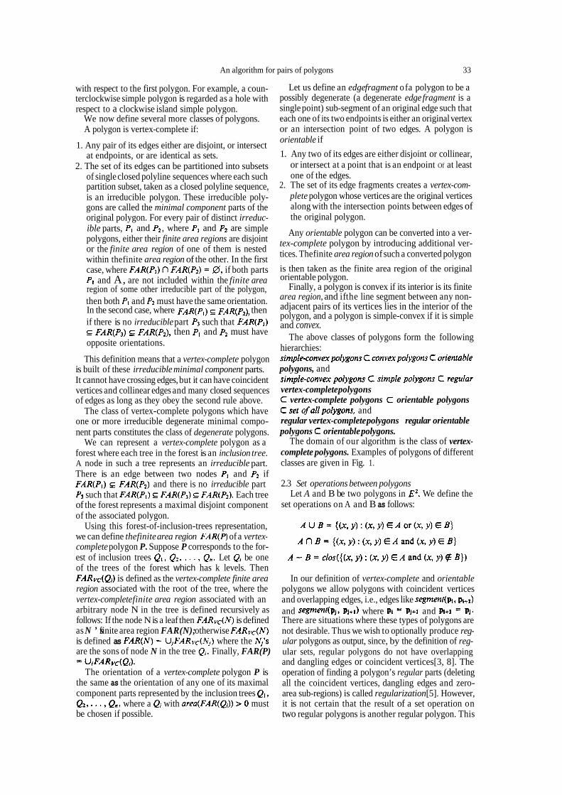
The domain of our algorithm is the class of vertex- complete polygons. Examples of polygons of different classes are given in Fig. 1.

2.3 Set operations between polygons

set operations on A and B as follows:

region of some other irreducible part of the polygon, area region, and if the line segment between any non-

then and must have The above classes of polygons form the following

Let A and B be two polygons in We define the

In our definition of vertex-complete and orientable polygons we allow polygons with coincident vertices and overlapping edges, i.e., edges like and where and There are situations where these types of polygons are not desirable. Thus we wish to optionally produce regular polygons as output, since, by the definition of regular sets, regular polygons do not have overlapping and dangling edges or coincident vertices[3, 8]. The operation of finding a polygon’s regular parts (deleting all the coincident vertices, dangling edges and zero- area sub-regions) is called regularization[5]. However, it is not certain that the result of a set operation on two regular polygons is another regular polygon. This

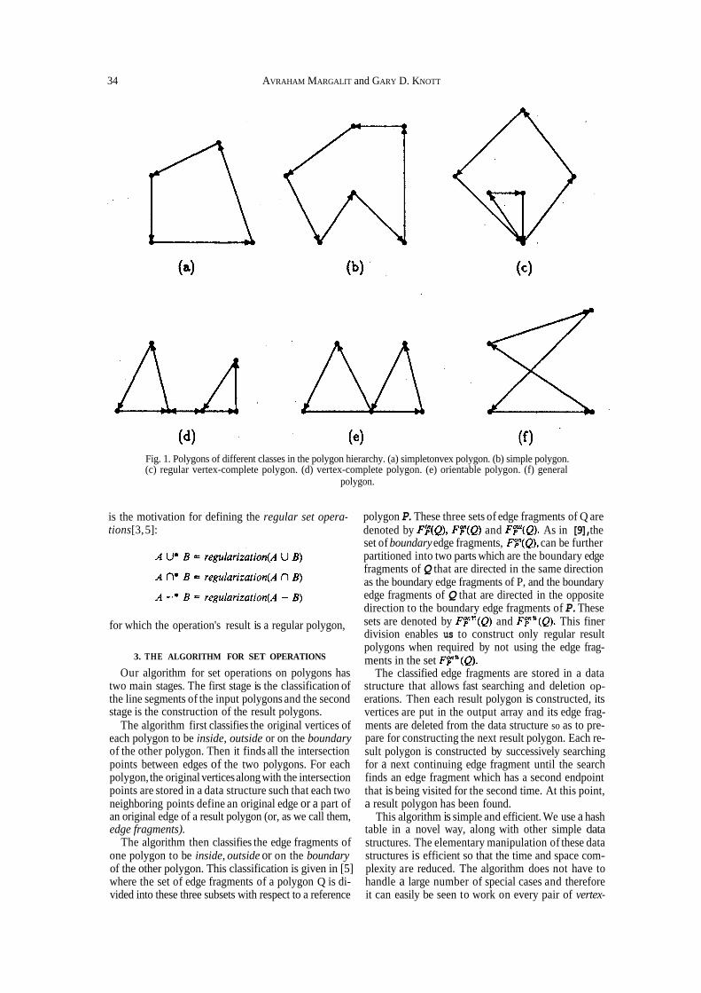
Fig. 1. Polygons of different classes in the polygon hierarchy. (a) simpletonvex polygon. (b) simple polygon. (c) regular vertex-complete polygon. (d) vertex-complete polygon. (e) orientable polygon. (f) general

polygon.

is the motivation for defining the regular set operations[3, 5]:

polygon P. These three sets of edge fragments of Q are denoted by and As in [9], the set of boundary edge fragments, can be further partitioned into two parts which are the boundary edge fragments of Q that are directed in the same direction as the boundary edge fragments of P, and the boundary edge fragments of Q that are directed in the opposite direction to the boundary edge fragments of P. These

division enables us to construct only regular result polygons when required by not using the edge fragments in the set

The classified edge fragments are stored in a data structure that allows fast searching and deletion operations. Then each result polygon is constructed, its vertices are put in the output array and its edge fragments are deleted from the data structure so as to pre- pare for constructing the next result polygon. Each result polygon is constructed by successively searching for a next continuing edge fragment until the search finds an edge fragment which has a second endpoint that is being visited for the second time. At this point, a result polygon has been found.

This algorithm is simple and efficient. We use a hash table in a novel way, along with other simple data structures. The elementary manipulation of these data structures is efficient so that the time and space complexity are reduced. The algorithm does not have to handle a large number of special cases and therefore it can easily be seen to work on every pair of vertex-

for which the operation's result is a regular polygon, sets are denoted by and This finer

3. THE ALGORITHM FOR SET OPERATIONS

Our algorithm for set operations on polygons has two main stages. The first stage is the classification of the line segments of the input polygons and the second stage is the construction of the result polygons.

The algorithm first classifies the original vertices of each polygon to be inside, outside or on the boundary of the other polygon. Then it finds all the intersection points between edges of the two polygons. For each polygon, the original vertices along with the intersection points are stored in a data structure such that each two neighboring points define an original edge or a part of an original edge of a result polygon (or, as we call them, edge fragments).

The algorithm then classifies the edge fragments of one polygon to be inside, outside or on the boundary of the other polygon. This classification is given in [5] where the set of edge fragments of a polygon Q is divided into these three subsets with respect to a reference



sified as a boundary point and inserted into both the vertex rings A V and BV in the proper places. If the intersection is along a common line segment, the two endpoints of the common segment are classified as boundary points and inserted into the two vertex rings in the right places.

However, the vertex ring insertion process inserts a new point only if this point does not exist or exists only once in the vertex ring. Thus a vertex can appear twice in sequence in a vertex ring, but no more copies will be stored. This allows the non-regular intersection of two polygons which intersect at just a single vertex to be correctly computed. Every two neighboring points in the vertex data structures represent an edge fragment which is a part of, or is equal to, an edge in the original polygon.

Each edge fragment belonging to one polygon is now classified to be inside, outside, or on the boundary of the other polygon. An edge fragment is defined to be inside if at least one of its endpoints is an inside vertex, or the two endpoints are boundary vertices but all the other points of the edge fragment are inside points (in this latter case it is enough to check if an internal point of the edge fragment is inside the other polygon). An edge fragment is defined to be outside if at least one of its endpoints is an outside vertex, or the two endpoints are boundary vertices but all the other points of the edge fragment are outside points (in this latter case it is enough to check if an internal point of the edge fragment is outside the other polygon). An edge fragment is a boundary fragment if all of its points are on the boundary of the other polygon.

Select the edge fragments from among the total set of edge fragments of both polygons, which are given implicitly in their respective vertex rings, as required to construct the result polygons. The required edge fragments to be selected depend on the specified set operation and the polygon types. These selected edge fragments are stored in an edge fragments table, EF. Each selected edge fragment from a given polygon is stored only once in the edge fragments table.

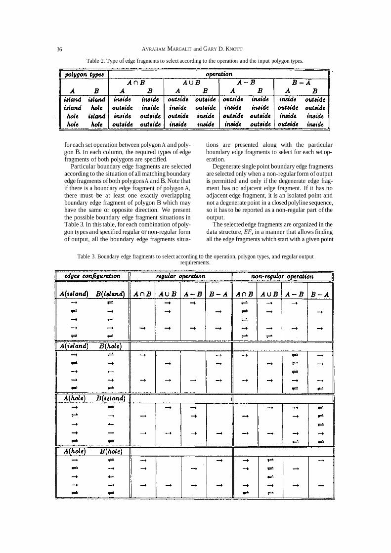
In the selection process the inside or outside edge fragments of both polygons are selected according to the operation and the two polygon types as summarized in Table 2. In this table there is a row for each combination of polygon types and a column

complete polygons, even those with vertices of degree more than two or with collinear edges.

3.1 General description of the algorithm The algorithm we use to solve the problem of com-

puting the result of a set operation on two polygons gets as its input an operation code which specifies whether union, intersection or set difference is desired, an indicator. code specifying .whether regular result polygons are required, and two vertex-complete polygon arrays, A and B, along with their types (island or hole). The algorithm constructs a set of irreducible result polygons along with their types in the output array C.

If regular output is not desired, various result polygons may be degenerate. A degenerate polygon is a point or a line segment given by oppositely directed overlapping edges. A point can be the result of a set intersection operation on two polygons, for example the intersection of two polygons that touch only at one vertex.

1. Normalize the orientations of the input polygons.

4. Classify the edge fragments.

The algorithm has six steps:

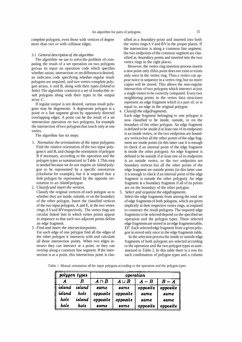
Find the relative orientation of the two input polygons A and B, and change the orientation of polygon B if necessary, according to the operation and the polygon types as summarized in Table 1. This step is needed because we do not require an island polygon to be represented by a specific onentation (clockwise for example), but it is required that a hole polygon be represented by the opposite orientation to an island polygon.

2. Classify and insert the vertices. Classify the original vertices of each polygon as to whether they are inside, outside, or on the boundary of the other polygon. Insert the classified vertices of the two input polygons, A and E, in the two vertex rings, AV and BV respectively. The vertex rings are circular linked lists in which vertex points appear in sequence so that each two adjacent points define an edge fragment.

For each edge of one polygon find all the edges of the other polygon it intersects with and calculate all those intersection points. When two edges intersect they can intersect at a point, or they can overlap along a common line segment. If the intersection is at a point, this intersection point is clas-

5 . Select and organize the edge fragments.

3. Find and insert the intersection points.

Table 1. Mutual orientation of the input polygons according to the operation and the polygon types.


Table 2. Type of edge fragments to select according to the operation and the input polygon types.

for each set operation between polygon A and poly- tions are presented along with the particular gon B. In each column, the required types of edge boundary edge fragments to select for each set op- fragments of both polygons are specified. eration.

Particular boundary edge fragments are selected Degenerate single point boundary edge fragments according to the situation of all matching boundary are selected only when a non-regular form of output edge fragments of both polygons A and B. Note that is permitted and only if the degenerate edge frag- if there is a boundary edge fragment of polygon A, ment has no adjacent edge fragment. If it has no there must be at least one exactly overlapping adjacent edge fragment, it is an isolated point and boundary edge fragment of polygon B which may not a degenerate point in a closed polyline sequence, have the same or opposite direction. We present so it has to be reported as a non-regular part of the the possible boundary edge fragment situations in output. Table 3. In this table, for each combination of poly- The selected edge fragments are organized in the gon types and specified regular or non-regular form data structure, EF, in a manner that allows finding of output, all the boundary edge fragments situa- all the edge fragments which start with a given point

Table 3. Boundary edge fragments to select according to the operation, polygon types, and regular output requirements.


The procedure polygonoperation uses the following and that allows any specified edge fragment to be deleted. We shall discuss later several options for the implementation of this data structure.

To construct each result polygon, we arbitrarily choose one edge fragment from the EF table and then successively choose an arbitrary edge fragment whose first endpoint matches the second endpoint of the previously chosen edge fragment. This process continues until an edge fragment is chosen whose second endpoint is now visited a second time (an irreducible polygon has now been found). Then the successive vertices of the polygon that was found are transferred in sequence to the output array as a single polygon and the corresponding edge fragments are deleted from the EF table whereupon another result polygon may be sought.

By using this method we form the greatest pos-

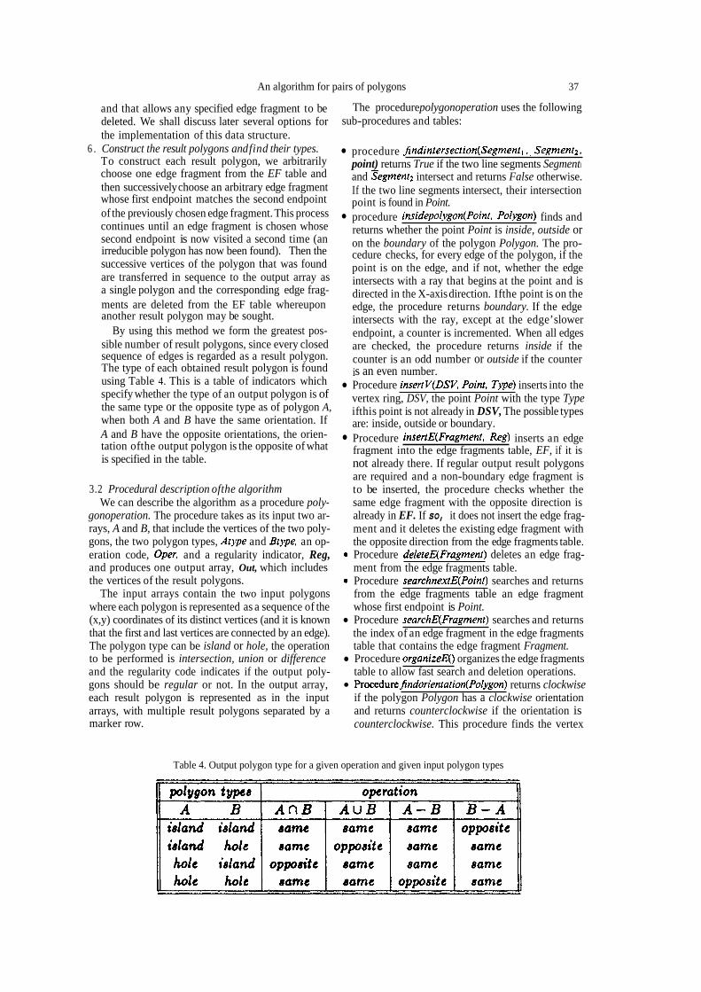
sequence of edges is regarded as a result polygon. The type of each obtained result polygon is found using Table 4. This is a table of indicators which

sub-procedures and tables:

procedure point) returns True if the two line segments Segmentl

and intersect and returns False otherwise. If the two line segments intersect, their intersection point is found in Point. procedure finds and returns whether the point Point is inside, outside or on the boundary of the polygon Polygon. The procedure checks, for every edge of the polygon, if the point is on the edge, and if not, whether the edge intersects with a ray that begins at the point and is directed in the X-axis direction. If the point is on the edge, the procedure returns boundary. If the edge intersects with the ray, except at the edge’s lower endpoint, a counter is incremented. When all edges

counter is an odd number or outside if the counter is an even number. Procedure inserts into the

6 . Construct the result polygons and find their types.

sible number of result polygons, since every closed are checked, the procedure returns inside if the

specify whether the type of an output polygon is of the same type or the opposite type as of polygon A,

vertex ring, DSV, the point Point with the type Type if this point is not already in DSV, The possible types

when both A and B have the same orientation. If A and B have the opposite orientations, the orien-

is specified in the table.

are: inside, outside or boundary. Procedure inserts an edge

not already there. If regular output result polygons are required and a non-boundary edge fragment is to be inserted, the procedure checks whether the same edge fragment with the opposite direction is already in EF. If so, it does not insert the edge fragment and it deletes the existing edge fragment with the opposite direction from the edge fragments table. Procedure deletes an edge fragment from the edge fragments table. Procedure searches and returns from the edge fragments table an edge fragment whose first endpoint is Point. Procedure searches and returns the index of an edge fragment in the edge fragments table that contains the edge fragment Fragment. Procedure organizes the edge fragments table to allow fast search and deletion operations.

returns clockwise if the polygon Polygon has a clockwise orientation and returns counterclockwise if the orientation is counterclockwise. This procedure finds the vertex

tation of the output polygon is the opposite of what fragment into the edge fragments table, EF, if it is

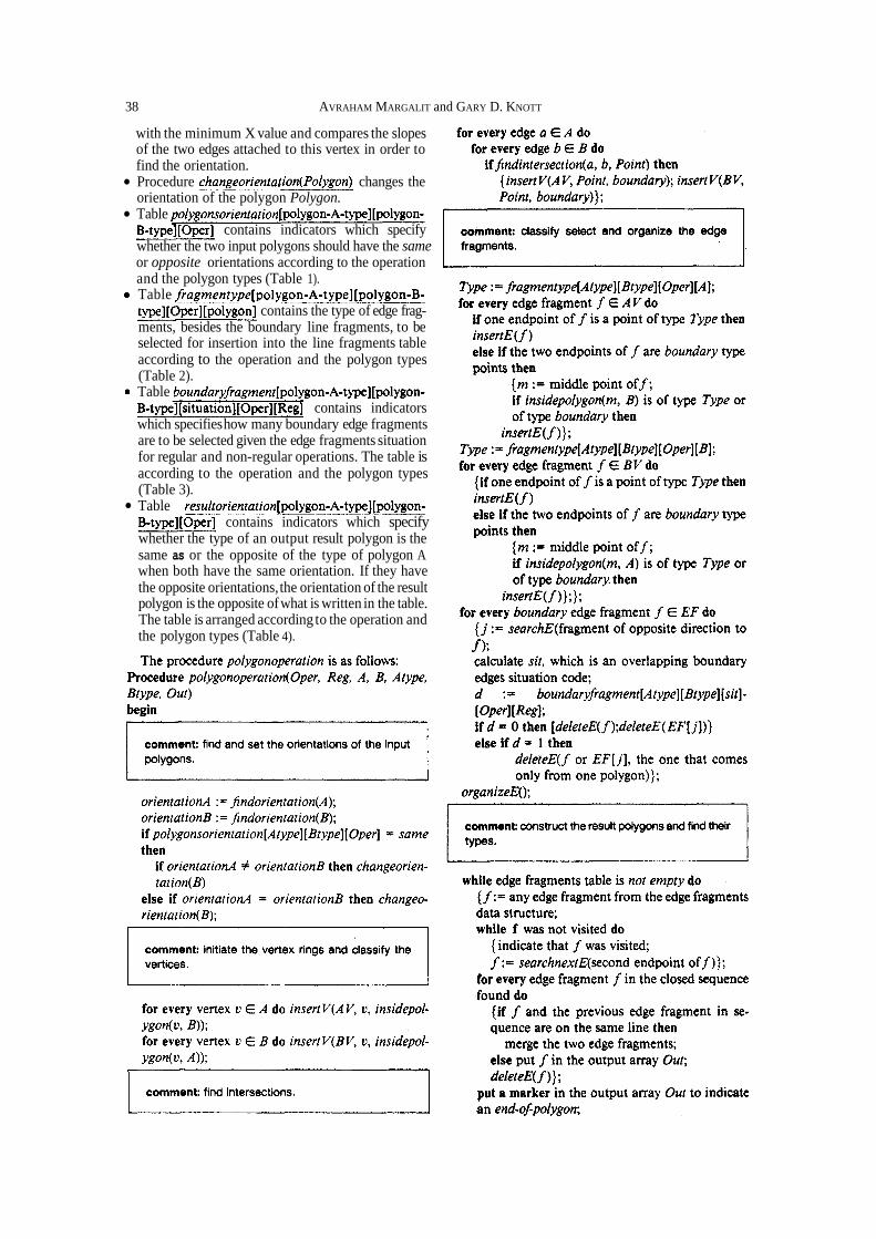
3.2 Procedural description ofthe algorithm We can describe the algorithm as a procedure poly-

gonoperation. The procedure takes as its input two arrays, A and B, that include the vertices of the two polygons, the two polygon types, and an operation code, and a regularity indicator, Reg, and produces one output array, Out, which includes the vertices of the result polygons.

The input arrays contain the two input polygons where each polygon is represented as a sequence of the (x,y) coordinates of its distinct vertices (and it is known that the first and last vertices are connected by an edge). The polygon type can be island or hole, the operation to be performed is intersection, union or difference and the regularity code indicates if the output polygons should be regular or not. In the output array, each result polygon is represented as in the input arrays, with multiple result polygons separated by a marker row.

Table 4. Output polygon type for a given operation and given input polygon types


with the minimum X value and compares the slopes of the two edges attached to this vertex in order to find the orientation. Procedure changes the orientation of the polygon Polygon. Table

contains indicators which specify whether the two input polygons should have the same or opposite orientations according to the operation and the polygon types (Table 1). Table

contains the type of edge fragments, besides the boundary line fragments, to be selected for insertion into the line fragments table according to the operation and the polygon types (Table 2). Table

contains indicators which specifies how many boundary edge fragments are to be selected given the edge fragments situation for regular and non-regular operations. The table is according to the operation and the polygon types (Table 3). Table

contains indicators which specify whether the type of an output result polygon is the same as or the opposite of the type of polygon A when both have the same orientation. If they have the opposite orientations, the orientation of the result polygon is the opposite of what is written in the table. The table is arranged according to the operation and the polygon types (Table 4).


from polygon A, polygon B or both. When both bits are set, the edge fragment is a boundary edge fragment of both polygons.

5. Two bits to store the edge fragment's type (inside, outside, or boundary) of the edge fragment whose first endpoint is in the current entry.

6. An index that is used in the construction of the result polygons to point to the next hash table entry used in the current attempt to construct a result polygon.

Insertion of an edge fragment is done first by finding an entry, for the second endpoint in the hash table (if it does not exist in the table, it is inserted). Then we find an entry for the first endpoint (if it does not exist in the table, or if it exists but its successor index is not - 1 then a new entry for is made). Then the successor index in is set to point to A single point edge fragment is inserted as one entry in the table where the successor index to the second endpoint points to the entry itself.

Deletion of an edge fragment is implemented by setting to -1 the successor index field in the entry of the first endpoint of the edge fragment.

Searching for an edge fragment is done by using linear open addressing hashing for an entry with the edge fragment’s first endpoint coordinates. If such an entry is found, the successor index field is checked for the second endpoint of the edge fragment. If the successor index field is not - 1, the edge fragment is found. If the successor index field is - 1, then the linear search continues until it is determined that no such point is stored.

All the boundary edge fragments of both polygons are inserted into the edge fragments table, EF, from the two vertex rings A V and BV. Then, for each boundary edge fragment for which one or more exactly overlapping edge fragments exist, the boundary situation is checked and some or all of these edge fragments are deleted, if necessary, according to Table 3.

When EF is implemented as a sorted table, this regularization process can & done by sorting the EF table after the insertion of the edge fragments of the first polygon, A, and then using binary search for the check discussed above, when inserting the edge fragments of the second polygon, B. After appending the admissible edge fragments from B, the whole EF array is sorted again.

When EF is implemented as a hash table, the edge fragments of A are inserted one-by-one with the hashing insertion procedure. Then, when the edge fragments of B are inserted, the search for oppositely directed edge fragments is done by hashing. The admissible edge fragments of B are inserted by hashing as soon as they are encountered.

In case a non-regular output is permitted, the procedure may produce output result polygons which are line-segment polygons (like a polygon whose edges are

and and/or single- point polygons (like a polygon whose edge is

along with any regular result polygons.

3.3 Implementation details In this section we describe the data structures and

methods used in implementing the procedure for set operations on polygons.

The procedure uses two linked lists, AV and BV, one array, EF, and three static control tables as its internal data structures.

The two linked lists are the vertex rings. They are used to store the vertices and intersection points of each polygon in sequential order, so that all edge frag- merits are defined by two adjacent vertex ring entries. The insertion of the original vertices of a polygon is done by linking them together into the linked list in their Original order (including the link between the last Vertex and the first one). The insertion of each intersection point is then done by moving along the linked list between the two original endpoints of the inter- sected edge and looking for the right place to insert the new intersection point according to the coordinates of the new point, the coordinates of the existing points and the edge direction.

We have imlemented the EF table, which is searched to construct the result polygons, using two different methods. In the first method EF is built as a sorted table. Each new edge fragment is inserted into the next available space in the array and subsequently the array is sorted. The search method used within this sorted EF table is binary search. Deletion of an edge fragment is handled by using one bit in each entry of the EF table to mark the entry as deleted or not deleted. This is done to avoid physical deletions that could require moving a lot of the entries.

In the second method, the EF table is built as an open addressing hash table of edge fragments. An entry in the hash table represents an endpoint of an edge fragment and contains the following fields:

1. A bit to indicate whether the entry is free or used. 2. The coordinates of an endpoint of the edge frag-

ment. 3. A successor index to the hash table entry that con-

tains the coordinates of the second endpoint of the edge fragment. If this successor index is -1, the current entry represents the terminating endpoint of an edge fragment and does not itself represent the first endpoint of an edge fragment.

4. Two bits to indicate whether the edge fragment whose first endpoint is in the current entry comes


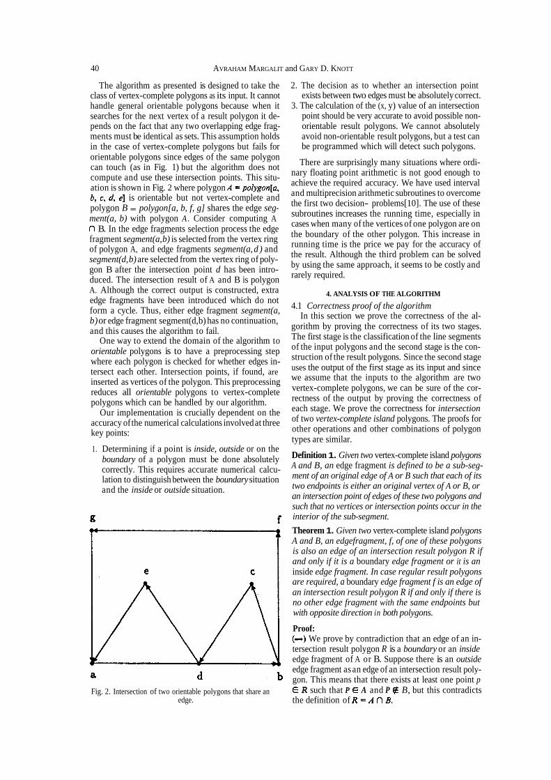
The algorithm as presented is designed to take the class of vertex-complete polygons as its input. It cannot handle general orientable polygons because when it searches for the next vertex of a result polygon it depends on the fact that any two overlapping edge fragments must be identical as sets. This assumption holds in the case of vertex-complete polygons but fails for orientable polygons since edges of the same polygon can touch (as in Fig. 1) but the algorithm does not compute and use these intersection points. This situation is shown in Fig. 2 where polygon

is orientable but not vertex-complete and

ment(a, b) with polygon A . Consider computing A B. In the edge fragments selection process the edge

fragment segment(a, b) is selected from the vertex ring of polygon A, and edge fragments segment(a, d ) and segment(d, b) are selected from the vertex ring of polygon B after the intersection point d has been introduced. The intersection result of A and B is polygon A. Although the correct output is constructed, extra edge fragments have been introduced which do not form a cycle. Thus, either edge fragment segment(a, b) or edge fragment segment(d, b) has no continuation, and this causes the algorithm to fail.

One way to extend the domain of the algorithm to orientable polygons is to have a preprocessing step where each polygon is checked for whether edges intersect each other. Intersection points, if found, are inserted as vertices of the polygon. This preprocessing reduces all orientable polygons to vertex-complete polygons which can be handled by our algorithm.

Our implementation is crucially dependent on the accuracy of the numerical calculations involved at three key points:

1. Determining if a point is inside, outside or on the boundary of a polygon must be done absolutely correctly. This requires accurate numerical calculation to distinguish between the boundary situation and the inside or outside situation.

2. The decision as to whether an intersection point exists between two edges must be absolutely correct.

3. The calculation of the (x, y) value of an intersection point should be very accurate to avoid possible non- orientable result polygons. We cannot absolutely avoid non-orientable result polygons, but a test can be programmed which will detect such polygons.

There are surprisingly many situations where ordi- nary floating point arithmetic is not good enough to achieve the required accuracy. We have used interval and multiprecision arithmetic subroutines to overcome the first two decision- problems[10]. The use of these

cases when many of the vertices of one polygon are on the boundary of the other polygon. This increase in running time is the price we pay for the accuracy of the result. Although the third problem can be solved by using the same approach, it seems to be costly and rarely required.

polygon B = polygon[a, b, f, g] shares the edge seg- subroutines increases the running time, especially in

4. ANALYSIS OF THE ALGORITHM

4.1 Correctness proof of the algorithm In this section we prove the correctness of the al-

gorithm by proving the correctness of its two stages. The first stage is the classification of the line segments of the input polygons and the second stage is the construction of the result polygons. Since the second stage uses the output of the first stage as its input and since we assume that the inputs to the algorithm are two vertex-complete polygons, we can be sure of the correctness of the output by proving the correctness of each stage. We prove the correctness for intersection of two vertex-complete island polygons. The proofs for other operations and other combinations of polygon types are similar.

Definition 1. Given two vertex-complete island polygons A and B, an edge fragment is defined to be a sub-segment of an original edge of A or B such that each of its two endpoints is either an original vertex of A or B, or an intersection point of edges of these two polygons and such that no vertices or intersection points occur in the interior of the sub-segment.

Theorem 1. Given two vertex-complete island polygons A and B, an edgefragment, f, of one of these polygons is also an edge of an intersection result polygon R if and only if it is a boundary edge fragment or it is an inside edge fragment. In case regular result polygons are required, a boundary edge fragment f is an edge of an intersection result polygon R if and only if there is no other edge fragment with the same endpoints but with opposite direction in both polygons.

Proof: We prove by contradiction that an edge of an in-

tersection result polygon R is a boundary or an inside edge fragment of A or B. Suppose there is an outside edge fragment as an edge of an intersection result polygon. This means that there exists at least one point p R such that P A and P B, but this contradicts

the definition of Fig. 2. Intersection of two orientable polygons that share an

edge.


sumption that both A and B are identically oriented.

Theorem 2. Given two identically oriented vertex-complete island polygons A and B, the set of all their inside and boundary edge fragments can be partitioned into edge-disjoint non-self-intersecting cycles of edge fragments where no two cycles share an edgefragment.

Proof: Define a polyline sequence of edge fragments as an ordered list of edge fragments where the second endpoint of each edge fragment is equal to the first endpoint of the next edge fragment in the list. We will prove the theorem by showing that every maximal sequence of inside and boundary edge fragments must form a cycle of edge fragments and that these cycles are edge-disjoint.

We first show that every maximal sequence of inside and boundary edge fragments must form a cycle. Sup- pose this is not true, so there is a maximal sequence of edge fragments that does not form a cycle. By Lemma 1 we know that every inside or boundary edge fragment has a continuation so this sequence must be infinite. But the number of edge fragments is finite, so such a sequence cannot exist.

Therefore, we see that every maximal sequence of inside and boundary edge fragments forms a cycle. If the cycle includes all the edge fragments of the sequence, we are done. If the cycle does not include all the edge fragments of the sequence, then we are left with a leading path of edge fragments, and we must show that this leading path has a continuation which is edge-disjoint from the cycle; then we can ensure that another cycle will be formed if the remaining sequence of edge fragments is continued using the successive continuation edge fragments of the leading path. We will show that the leading path has a continuation by considering all the possible cases.

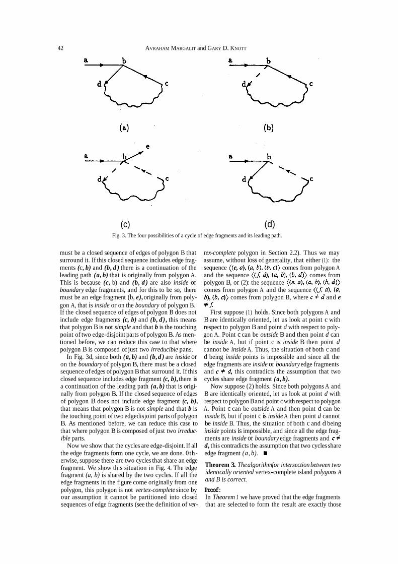
In Fig. 3 we show the four different cases for a leading path and a cycle. The solid lines represent edge fragments that are originally from polygon A and the dashed lines represent edge fragments that are originally from polygon B. In the figure, edge fragment (a, b) is the leading path while the sequence

is the cycle. In Fig. 3(a) and 3(b), vertex b has an indegree of two. That means that polygon A is not simple and that b is a touching point of two edge-disjoint parts of polygon A.

Now, if a vertex-complete polygon A consists of two edgedisjoint parts with some common vertices, the result of the intersection of such a polygon with another polygon B can be considered as the union of the intersection results of the edge-disjoint cycles of A with B. Thus, we can consider these two intersection s u b problems separately. This reduction process may be reiterated until both parts of A are irreducible parts. Thus, we may assume we have the base case where polygon A is formed from exactly two irreducible parts.

In Fig. 3c, since edge fragment (a, b) is originally an inside or a boundary edge fragment of polygon A , there

We prove by contradiction that a boundary or an inside edge fragment of A or B is an edge in the intersection result polygon R. Suppose there is a boundary or an inside edge fragment of A that is not an edge in the result polygon R. This means that there is a point

This contradicts the definition of

Now we prove by contradiction that the boundary edge fragments that contribute to a regular intersection result polygon are those that appear only in one direction. From the previous part of the proof we know that every boundary edge fragment of A and B appears in a possibly non-regular result polygon R. So if a boundary edge fragment appears twice in both directions, it contributes two opposite directed edges to a result polygon. Such a result polygon is not a regular polygon since it includes overlapping edges. Thus, the edge fragments that contribute to a regular result polygon cannot be those that appear in both directions; they must be those that appear only in one direction.

Lemma 1. Given two vertex-complete island identically oriented input polygons A and B, for every inside or boundary edge fragment selected for constructing an intersection result polygon, there is a continuation edge fragment which is an input edge fragment or a boundary edge fragment.

Proof: We prove this lemma by considering all the possible inside or boundary edge fragments. Case 1 : is an inside edge fragment. In this case is either an inside point or a boundary point. If is an inside point, it is an original vertex of one of the polygons (suppose, without loss of generality, it is an original vertex of polygon A) so there is an original edge of A , such that at least a part of it is inside B. Thus, there is a continuation edge fragment, that is a part of edge where

is either or is a point on the edge that is an intersection point between and an edge of polygon B.

If pi is a boundary point let us assume, without loss of generality, that is an edge fragment that is originally from polygon A . If is an original vertex of polygon A and the next edge fragment of A is inside or on the boundary of polygon B, we are done. If the next edge fragment of A is outside of polygon B or is an intersection point, there is a part of the edge of polygon B that is on that is inside polygon A , so there is an edge fragment that is originally from polygon B, that can continue edge fragment Case 2: is a boundary edge fragment. Inthiscase is an edge fragment of both A and B. If A and B continue to have the same boundary,

is a boundary edge fragment that continues If after point one of the polygons, A or B,

goes inside the other one, there is an inside continuation edge fragment. If after point both the polygons go outside each other, then the two polygons have opposite orientations, and this contradicts the as-


(c) (d) Fig. 3. The four possibilities of a cycle of edge fragments and its leading path.

must be a closed sequence of edges of polygon B that tex-complete polygon in Section 2.2). Thus we may surround it. If this closed sequence includes edge frag- assume, without loss of generality, that either (1): the ments (c, b) and (b, d ) there is a continuation of the sequence comes from polygon A leading path (a, b) that is originally from polygon A. and the sequence comes from This is because (c, b) and (b, d ) are also inside or polygon B, or (2): the sequence boundary edge fragments, and for this to be so, there comes from polygon A and the sequence must be an edge fragment (b, e), originally from poly- comes from polygon B, where and e gon A, that is inside or on the boundary of polygon B. If the closed sequence of edges of polygon B does not First suppose (1) holds. Since both polygons A and include edge fragments (c, b) and (b, d) , this means B are identically oriented, let us look at point c with that polygon B is not simple and that b is the touching respect to polygon B and point d with respect to poly- point of two edge-disjoint parts of polygon B. As men- gon A. Point c can be outside B and then point d can tioned before, we can reduce this case to that where be inside A, but if point c is inside B then point d polygon B is composed of just two irreducible pans. cannot be inside A. Thus, the situation of both c and

In Fig. 3d, since both (a, b) and (b, d ) are inside or d being inside points is impossible and since all the on the boundary of polygon B, there must be a closed edge fragments are inside or boundary edge fragments sequence of edges of polygon B that surround it. If this and this contradicts the assumption that two closed sequence includes edge fragment (c, b), there is cycles share edge fragment (a, b). a continuation of the leading path (a, b) that is origi- Now suppose (2) holds. Since both polygons A and nally from polygon B. If the closed sequence of edges B are identically oriented, let us look at point d with of polygon B does not include edge fragment (c, b), respect to polygon Band point c with respect to polygon that means that polygon B is not simple and that b is A. Point c can be outside A and then point d can be the touching point of two edgedisjoint parts of polygon inside B, but if point c is inside A then point d cannot B. As mentioned before, we can reduce this case to be inside B. Thus, the situation of both c and d being that where polygon B is composed of just two irreduc- inside points is impossible, and since all the edge frag- ible parts. ments are inside or boundary edge fragments and

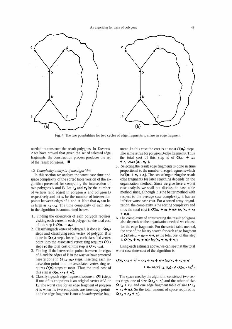
Now we show that the cycles are edge-disjoint. If all d, this contradicts the assumption that two cycles share the edge fragments form one cycle, we are done. 0th- edge fragment (a, b). erwise, suppose there are two cycles that share an edge

Theorem 3. The algorithm for intersection between two fragment. We show this situation in Fig. 4. The edge identically oriented vertex-complete island polygons A fragment (a, b) is shared by the two cycles. If all the and B is correct. edge fragments in the figure come originally from one

polygon, this polygon is not vertex-complete since by Proof: our assumption it cannot be partitioned into closed In Theorem 1 we have proved that the edge fragments sequences of edge fragments (see the definition of ver- that are selected to form the result are exactly those


Fig. 4. The two possibilities for two cycles of edge fragments to share an edge fragment.

needed to construct the result polygons. In Theorem 2 we have proved that given the set of selected edge fragments, the construction process produces the set of the result polygons.

4.2 Complexity analysis of the algorithm In this section we analyze the worst case time and

space complexity of the sorted table version of the algorithm presented for computing the intersection of two polygons A and B. Let and be the number of vertices (and edges) in polygon A and polygon B respectively and let be the number of intersection points between edges of A and B. Note that can be as large as The time complexity of each step in the algorithm is summarized below.

ment. In this case the cost is at most steps. The same is true for polygon B edge fragments. Thus the total cost of this step is of

5 . Selecting the result edge fragments is done in time proportional to the number of edge fragments which is The cost of organizing the result edge fragments for later searching depends on the organization method. Since we give here a worst case analysis, we shall not discuss the hash table method since, although it is the better method with respect to the average case complexity, it has an inferior worst case cost. For a sorted array organization, the complexity is the sorting complexity and thus the total cost is

also depends on the organization method we choose for the edge fragments. For the sorted table method,

is so the total cost of this step is

Using each estimate above, we can see that the total

1. Finding the orientation of each polygon requires 6. The complexity of constructing the result polygons visiting each vertex in each polygon so the total cost of this step is

steps and classifying each vertex of polygon B is done in steps. Inserting each classified vertex point into the associated vertex ring requires steps so the total cost of this step is

3. Finding all the intersection points between the edges of A and the edges of B in the way we have presented here is done in steps. Inserting each intersection point into the associated vertex ring requires steps at most. Thus the total cost of this step is

4. Classifying each edge fragment is done in steps if one of its endpoints is an original vertex of A or B. The worst case for an edge fragment of polygon A is when its two endpoints are boundary points and the edge fragment is not a boundary edge frag-

2. Classifying each vertex of polygon A is done in the cost of the binary search for each edge fragment

worst case time-cost of the algorithm is

The space used by the algorithm consists of two vertex rings, one of size and the other of size

and one edge fragment table of size So the total amount of space required is


By using modifications discussed below, an elabo- rated algorithm whose overall time cost is

can be obtained.

4.3 Improvements to the algorithm In this section we discuss some theoretical, but pos-

sibly impractical, improvements to the algorithm. We can see in the previous section that the largest contri- butions to the worst case time complexity come from the cost of two steps of the algorithm:

Finding the intersection points of the edges of the

ring, continuing from point v, until a boundary point is found, assign all the edges visited to be inside edge fragments, and go to (4).

3. If all the points in the vertex ring, AV, are now visited, quit. Otherwise follow the points in the A V ring, continuing from point v, until a boundary point is found, and assign all the edges visited to be outside edge fragments.

4. If all the points in the vertex ring, AV, are now visited, quit. Otherwise continue to follow the points in the A V ring until all points are visited or until this step is exited while checking the edges in the

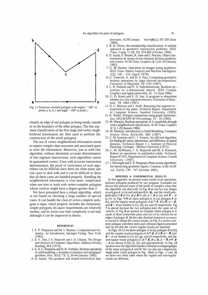
boundary points and they lie on one edge of B, they form a boundary edge fragment. If one point, u, is a boundary point that is an intersection point of edges and and if this intersection point is not an endpoint of and if the next point, w, is to the east of then classify the edge fragment (u, w) as an inside edge fragment and go to (2). If the next point, w, is to the west of then classify the edge fragment (u, w) as an outside edge fragment and go to (3). In case the first point, u, is an endpoint of b, we have to check whether the second point is to the east or west of both and and take into consideration the angle between . We and summarize the rules in Table 5 . If the edge fragment is seen to be an inside edge fragment, classify it as such and go to (2). If the edge fragment is seen to be an outside edge fragment, classify it as such and go to (3).

We present Fig. 5 to help clarify the meaning of angles that are greater or less than 180°.

In step (1) the algorithm visits once, in the worst case, each node of the vertex ring AV. In steps (2)-(4)

A V. For each edge fragment in A V it checks if the edge

of polygon B. Thus, this classification algorithm requires time.

two polygons and inserting them into the vertex reference polygon B. If two adjacent points are rings. Classifying the edge fragments as inside, outside, or boundary edge fragments.

For the first of these problems, we can theoretically use the algorithm sketched by Mairson and Stolfi[ 11] to find the intersection points. Given two sets of line segments A and B, consisting of and noninter- secting segments respectively, this algorithm finds all the intersection points of segments of A with segments of B in time. Now, to handle the insertions, we can put the intersection points in a temporary array, sort the array according to the coordinates of the endpoints and the direction of the original edge, and then form the vertex ring by traversing the sorted array. This insertion sub- computation will take time.

For the second problem we can use an algorithm to classify the edge fragments in which we first find the intersection points and insert them into the vertex rings, and then classify the edge fragments using the information that intersection points are boundary points. We present here a brief description of this classification

reference polygon B. In the case of a counterclockwise

as follows:

1. Choose from the vertex ring, A V, an original vertex, v , that is not a boundary point, and find if it is an

to (2) and if it is an outside point go to (3). If there is no such vertex v (i.e., all the vertices of polygon A are boundary points) choose one vertex v of A and go to (4).

2. If all the points in the vertex ring, A V, are now visited, quit. Otherwise follow the points in the A V

algorithm for a clockwise oriented polygon A and a the algorithm visits once each node of the vertex ring

polygon the algorithm is similar. The algorithm goes fragment is to the east or the west of at most two edges

inside or an outside point. If it is an inside point go 5. CONCLUSIONS As mentioned before, algorithms for set operations

on polygons usually have two main stages: edge classification and output polygon construction.

A common approach to the classification problem is the use of a divide and conquer paradigm along with vertex neighborhood information[5,8] in order to

Table 5. The rules when the first point of edge fragment (u, w ) is an endpoint of


structures. ACM Comput. Surveys 16(2), 187-260 (June 1984).

5. R. B. Tilove, Set membership classification: A unified approach to geometric intersection problems. IEEE Trans. Comp. C-29( 10), 874-883 (October 1980).

6. D. Ayala, P. Brunet, R. Juan and I. Navazo, Object representation by means of non-minimal division quadtrees and octrees. ACM Trans. Graphics 4( 1),41-59 (January 1985).

7. G. M. Hunter, Operation on images using quadtrees. IEEE Trans. Pattern Analysis and Machine Intelligence

8. G. Vanecek, Jr. and D. S. Nau, Computing geometric boolean operations by input directed decomposition, University of Maryland, TR 1762 (1987).

9. L. K. Putnam and P. A. Subrahmanyam, Boolean op - erations on n-dimensional objects. IEEE Comput. Graphics and Applications 6(6), 43 - 51 (June 1986).

10. G. D. Knott and E. D. Jou, A program to determine whether two line segments intersect, University of Mary- land, TR 1884 (1987).

11. H. G. Mairson and J. Stolfi, Reporting line segment in - tersections in the plane, Technical Report, Department of Computer Science, Stanford University, (1983).

12. K. Weiler, Polygon comparison using graph representa - tion, SIGGRAPH 80 Proceedings, 10 - 18 (1980).

13. M. Mantyla, Boolean operations of 2- manifolds through vertex neighborhood classification. ACM Trans. Graphics 5( 1), 1-29 (January 1986),

14. M. Mantyla, Introduction to Solid Modeling, Computer Science Press, Rockville, MD (1987).

15. C. M. Eastman and C. J. Yessios, An efficient algorithm for finding the union, intersection, and difference of spatial domains, Technical Report 3 1, Institute of Physical Planning, Carnegie - Mellon University (1972).

16. C. M. Hoffmann, J . E. Hopcroft and M. S. Karasick, Robust set operations on polyhedral solids, Technical Report 87-875, Department of Computer Science, CornellUniversity (1987).

for intersecting geometric figures. Commun. of the ACM vol. 25(10), 739 - 747 (October 1982).

1(2), 145 - 153 (April 1979).

Fig. 5. Clockwise oriented polygon with angles < 180° at points a, b, d, e and angle > 180° at point c.

classify an edge of one polygon as being inside, outside or on the boundary of the other polygon, The line segment classification of the first stage and vertex neighborhood information are then used to perform the construction of the result polygons.

The use of vertex neighborhood information seems to require complex data structures and associated space to store the information. Moreover, just as with Our algorithm, without absolutely accurate determination of line segment intersections, such algorithms cannot

determination, the proof of correctness of such algorithms can be difficult since there are often many special cases to deal with and it can be difficult to show

neighborhood information is even more complicated

whose vertices might have a degree greater than 2. We have presented here a robust algorithm, which

is not based on checking a large number of special cases. It can handle the class of vertex-complete polygons as input, which properly includes the elementary simple polygons. Its space requirements are relatively modest, and its worst case time complexity is not bad, although it can be improved in theory.

be guaranteed correct. Even with accurate intersection 17. J. Nievergelt and F. P. Preparata, Plane-sweep algorithms

that all these cases are handled properly. Handling the APPENDIX A EXPERIMENTAL RESULTS In this appendix we present some results of set operations

between polygons produced by our program. Examples are

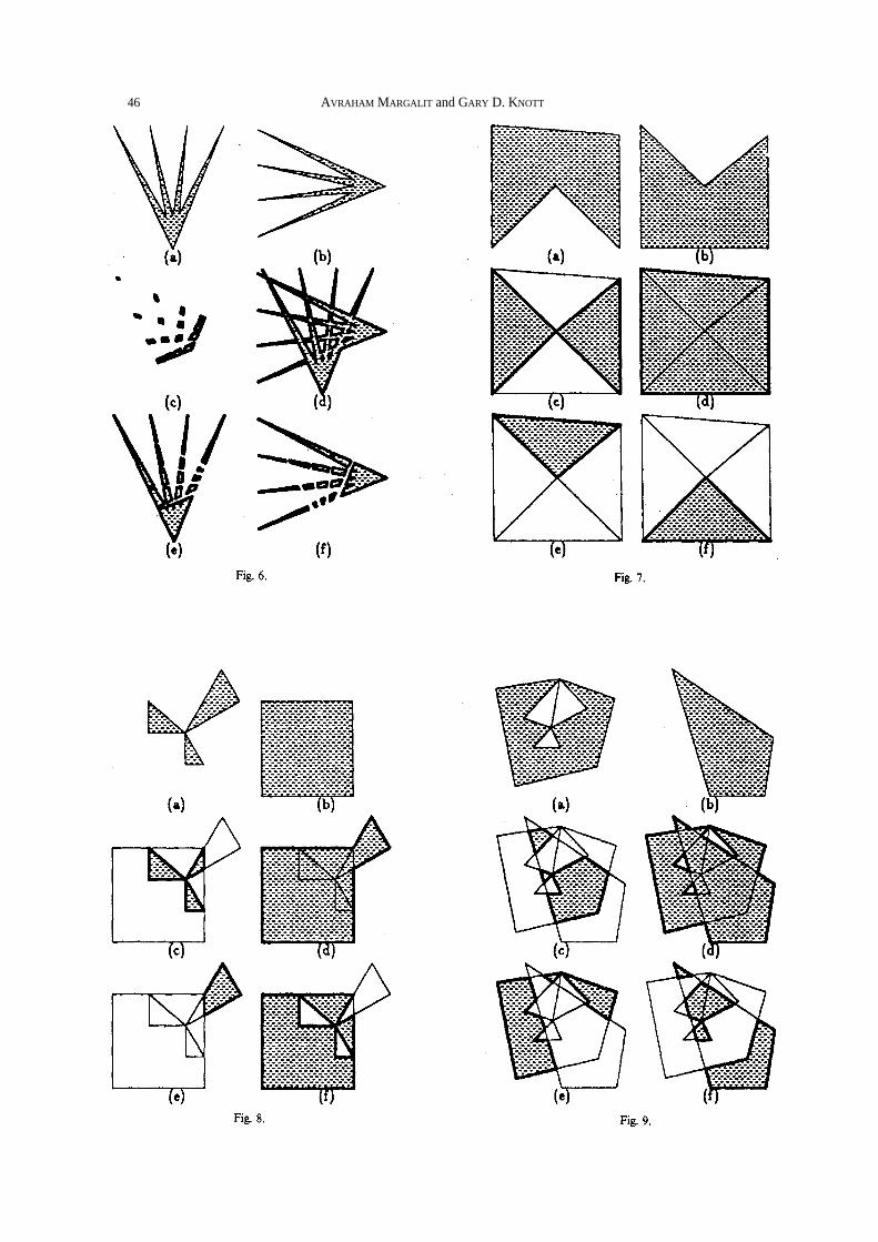
the algorithm can deal with. In Fig. 6 we see two star shapes as polygon A in (a) and polygon Bin (b), and the result polygons o f in (c), in (d), in (e), and in (f) in Figs. 7-9 we show polygon A in (a), polygon B in (b), and the regular result polygons of and are shaded in (c), (d), (e), and (f) respectively. Fig. 7 is special because the two polygons have the same set of vertices. In Fig. 8 we present an example where polygon A is made of three irreducible parts and two of its vertices lie on edges of polygon B. In this case absolute numerical accuracy is crucial to obtain the correct results. In Fig. 9 a vertex-complete polygon with three holes and collinear edges is presented and we see that the correct regular results are obtained.

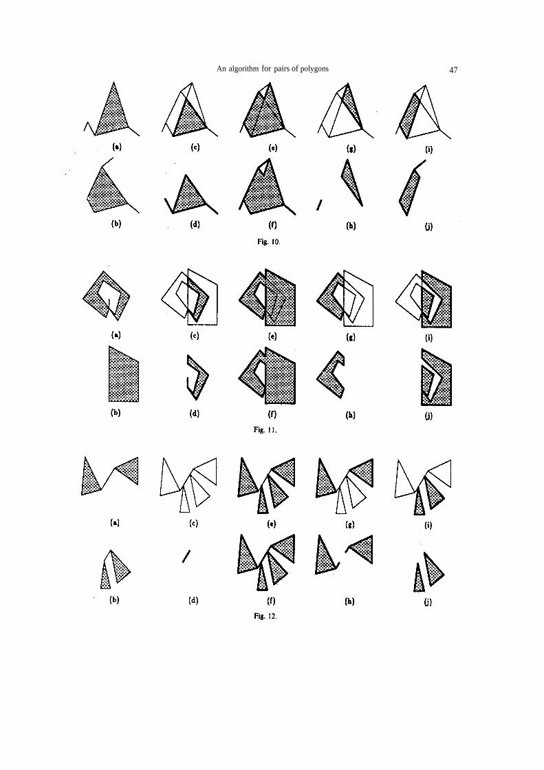
In Figs. 10-12 we show polygon A in (a), polygon B in (b), and the regular results polygons of and

are shaded in (c), (e), (g), and (i) respectively, and the non-regular result polygons of and

are shown in (d), (f), (h), and (j) respectively. In Fig. 10 we show how the algorithm handles collinear overlapping edges of the input polygons A and B. We can also see a degenerate single point result polygon in Fig. 10(d). in Figs. 1 1. and 12 we show two other cases where the regular and non-regular results are different.

when one tries to work with vertex-complete polygons shown that present some of the kinds of complex cases that

REFERENCES

1. F. P. Preparata and M. I. Shamos. Computational Ge- ometry, An Introduction, Springer-Verlag. New York (1985).

2. A. V. Aho, J. E. Hopcroft and J. D. Ullman, The Design and Analysis of Computer Algorithms, Addison-Wesley, Reading, MA (1974).

3. A. A. G. Requicha and H. B. Voelcker, Boolean operations in solid modeling-boundary evaluation and merging algorithms. Proc. IEEE 73( 1), 30-44 (January 1985).

4. H. Samet, The quadtree and related hierarchical data



Documents

AN ALGORITHM FOR COMPUTING THE UNION, INTERSECTION OR ...jarek/graphics/papers/04PolygonBooleansMargali… · AN ALGORITHM FOR COMPUTING THE UNION, INTERSECTION OR DIFFERENCE