Embed Size (px)
Citation preview
An Algorithm for Correction of Beam Hardening in Computerized X-Ray Tomography
K. K. Mishra, A. M. Quraishi, Shanta Mishra, Ashwani Kumar Atul Srivastava, K. Muralidhar1 and P. Munshi
Department of Mechanical Engineering
Indian Institute of Technology, Kanpur – 208 016
ABSTRACT
The paper reports a beam hardening correction algorithm to be applied on the polyenergetic projection data obtained during X-ray tomography of a specimen. Convolution back projection (CBP) algorithm has been used to reconstruct the cross-section of the specimen from the corrected projection data. The beam hardening correction has been applied on simulated test objects and the results have been found to be satisfactory. The number of energy levels taken into account is five for the considered test cases. The algorithm recovers one solution for each energy level. The distribution of errors in each of the solutions depends on the size of the energy level as well as the material density distribution.
Keywords: Beam hardening, X-ray tomography, convolution back projection, flaw detection.
1. INTRODUCTION
The technique of computerized tomography (CT) has established itself as a leading
tool in diagnostic radiology over the past three decades and is catching on rapidly in
the area of non-invasive measurements (NIM). According to Herman1, the aim of CT is
to obtain information regarding the nature of material occupying exact positions inside
the body. CT assigns a number to every point inside the body that corresponds to a
specific material property at that point. A suitable physical property for this number is
the X-ray or the γ-ray attenuation coefficient of the material. It is obtained from the
projection data recorded from an experiment. The reconstruction technique can be the
convolution back projection (CBP) algorithm, originally developed by Ramachandran
and Laxminarayanan2, or the algebraic reconstruction technique (ART)3,4. In the
present study, CBP has been used for the reconstruction of the projection data. It is
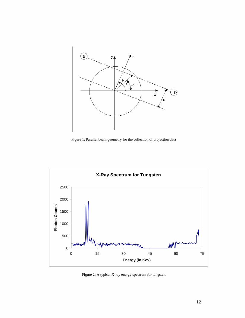
assumed that the data is available in a parallel beam configuration, Figure 1; this
approach has been discussed by Manzoor, et al5. The filter function used in all the
reconstructions of CBP is Hamming 54, a filter that resolves well the smooth variations
1 Author for correspondence. Manuscript under review.
2
in the attenuation coefficient and hence the density. For the purpose of displaying the
reconstructed image, the CT numbers are read from the CBP output file and
appropriate gray levels are assigned to it6. Thus by generating a gray scale for each of
the projection data, the CT image can be graphically displayed on a grid. For the correct reconstruction of the object, the input file to the CBP must contain
perfect projection values of the object. In the real life experiment, there are many
sources of imperfections in the recorded projection data. These include a finite source
and detector size, scattering of photons, and polyenergetic photons. The measured
projection data must be analytically corrected for all these imperfections before being
used for reconstruction. In the present work, corrections for the polyenergetic nature of
radiation are discussed. 2. THE PROBLEM OF BEAM HARDENING
Of the many sources of imperfections in the projection data referred above that
related to the polyenergetic nature of radiation is called beam hardening. An X-ray
source emits photons of multiple energies. A typical energy distribution (spectrum) for
an X-ray source (for example, tungsten) has been shown in Figure 2. The coefficient of
linear attenuation of the material is usually a function of the incident photon energy.
The attenuation at a fixed point is greater for the photons of lower energy. Hence the
energy distribution of the X-ray beam changes (hardens) as it passes through the
object. This effect is called the hardening of the X-ray beam. The X-ray beams
reaching the same point from different directions are likely to have different spectra
(having passed through different material before reaching this point) and thus will be
attenuated differently at that point. The coefficients of linear attenuation of a given
specimen recovered by a tomographic calculation are not the exact values at a given
energy. Instead they are a combination of attenuation coefficients emitted at all the
energies by the X-ray source. This combination depends upon the type of functional
dependence of the attenuation coefficient on the photon energy and the probabilistic
energy distribution of the source, i.e. temporal photon statistics. The coefficient of
linear attenuation can be mapped to specific properties of the material such as the
density distribution. Hence for non-destructive evaluation and non-invasive
measurements using computerized tomography (CT) to be reliable, it is necessary to
apply corrections for beam hardening. It requires the conversion of polyenergetic
3
projection data recorded in the experiments into monoenergetic projection data, before
reconstruction. In the present study, we have demonstrated beam hardening and its
correction by defining computer-generated objects and mathematically calculating the
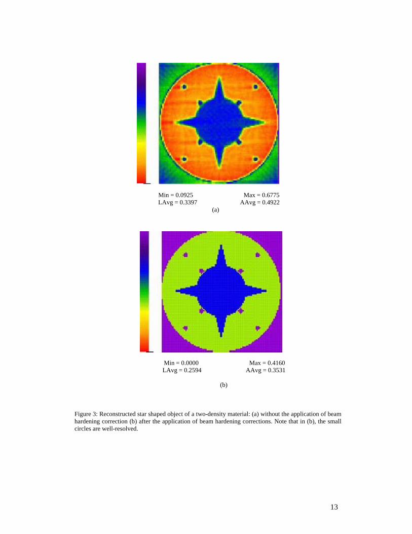
projection data for them. As an example a star shaped object comprising of two
materials is presented. For a resolution of 100 rays and 100 views, Figure 3(a) shows
the reconstruction without the application of beam hardening correction, and Figure
3(b) is a reconstruction after the application of beam hardening corrections. 3. BEAM HARDENING CORRECTION ALGORITHM
Herman1 has shown the exact correction for beam hardening in the context of
medical imaging when the reconstruction region has only two types of materials. An
algorithm for more than two types of materials was also proposed by Herman7,8. It was
modified by Rama Krishna9 for applications in NDT. In both cases the monoenergetic
reconstruction was carried out at the mean X-ray energy level and a systematic
assessment of errors was not attempted. In the present work, we propose an improved
algorithm for the correction of beam hardening where (1) the reconstruction can be
performed at any of the energies of the incoming radiations (2) the number of material
in the object is greater than two, and (3) the iteration scheme can be continued till the
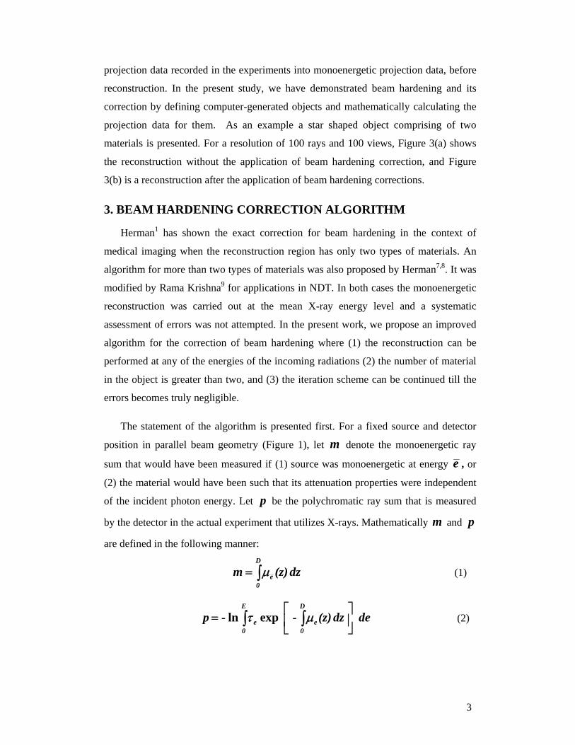
errors becomes truly negligible. The statement of the algorithm is presented first. For a fixed source and detector
position in parallel beam geometry (Figure 1), let m denote the monoenergetic ray
sum that would have been measured if (1) source was monoenergetic at energy e , or
(2) the material would have been such that its attenuation properties were independent
of the incident photon energy. Let p be the polychromatic ray sum that is measured
by the detector in the actual experiment that utilizes X-rays. Mathematically m and p
are defined in the following manner:
∫=D
0e dz (z) m μ (1)
de dz (z) - - pD
0e
E
0e ⎥
⎦
⎤⎢⎣
⎡= ∫∫ μτ expln (2)
4
Here D is the distance from the source to the detector, )z(eμ is the linear
attenuation coefficient at energy e at a point on the line from the center of the source
to the center of the detector at a distance z from the detector, E is the highest energy
level present in the beam, and eτ is the probability that a detected photon of the X-ray
beam (in air between the source and the detector) is at energy e . It is to be recalled
that in a complete NDT experiment, m and p represents two-dimensional images
with respect to the ray number and the angle of projection. Such images are called
sinograms5. Beam hardening correction can be done efficiently by performing a polynomial
curve fitting between the image data of m and p . In a real experiment we get only
the projection data p . Therefore to get a correlation between m and p we have to
generate a synthetic data set of m . To approximate the monoenergetic data set m , we
need prior (partial) information about the object. Hence as a first guess of the object,
we can use the direct reconstruction of the cross-section from the experimental data p
using CBP.
Let this approximation be 0O . Collecting a new set of relevant information
including the geometry and the size of the object from the reconstructed image, objects
iX can be generated at different selected energies from the X-ray source spectrum.
This step requires that the coefficients of linear attenuation at those energies for the
particular material be used. The coefficients of linear attenuation for various materials
can be obtained from handbooks, or can be obtained experimentally in a calibration
experiment by using a single line of the X-ray beam at a time. From the generated
objects iX , the approximate projection data im ’s can be obtained from Equation (3).
Even for a defect free sample im is different from im due to the discretization of the
reconstruction region. But if defects are present in the sample, then im will have
information about these defects. This important information will not be present im in
the first iteration.
5
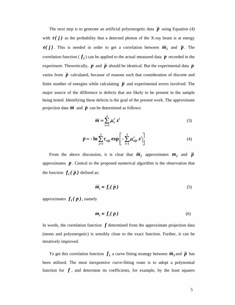
The next step is to generate an artificial polyenergetic data p using Equation (4)
with )j(τ as the probability that a detected photon of the X-ray beam is at energy
)j(e . This is needed in order to get a correlation between im and p . The
correlation function ( if ) can be applied to the actual measured data p recorded in the
experiment. Theoretically, p and p should be identical. But the experimental data p
varies from p calculated, because of reasons such that consideration of discrete and
finite number of energies while calculating p and experimental errors involved. The
major source of the difference is defects that are likely to be present in the sample
being tested. Identifying these defects is the goal of the present work. The approximate
projection data m and p can be determined as follows:
iI
1i
ie z m ∑
== μ (3)
⎥⎦⎤
⎢⎣⎡= ∑∑
==
I
1i
iie(j)
J
1je(j) z - - p μτ expln (4)
From the above discussion, it is clear that im approximates im and p
approximates p . Central to the proposed numerical algorithm is the observation that
the function )p(f i defined as:
)p(f m ii ≈ (5)
approximates )p(f i , namely
)p(f m ii ≈ (6)
In words, the correlation function f determined from the approximate projection data
(mono and polyenergetic) is sensibly close to the exact function. Further, it can be
iteratively improved. To get this correlation function if a curve fitting strategy between im and p has
been utilized. The most inexpensive curve-fitting route is to adopt a polynomial
function for f , and determine its coefficients, for example, by the least squares
6
technique. Any other image processing operation such as correlation and image
registration can also be employed. The corrections obtained and the number of
iterations required in each case will however be different. This function if obtained
after correlation can then be applied on the experimental data p to obtain the
equivalent monoenergetic projection data set im of the object under test as in
Equation (6). CT algorithms such as CBP can be applied to im .
The numerical algorithm can now be summarized as follows: The unknown object
cross-section is first assessed using polyenergetic data. The function if is estimated
with respect to this object. The first iterate of the correlation function is applied to the
experimentally recorded polyenergetic data of the test object. The first reconstruction
1iO is carried out using CBP from )p(f i as it approximates im . This completes
the first iteration of beam hardening correction. Using the individual monoenergetic
data sets, the cross-section can be repeatedly reconstructed (using, say CBP). The next
step is to compare with the initial guess 0O . If new features are visible, for example a
crack or the set of dislocations, the initial guess is improved accordingly and all the
steps are repeated again. If new features are not visible then the correction algorithm
will stop. The solutions obtained at different energies can now be displayed. The
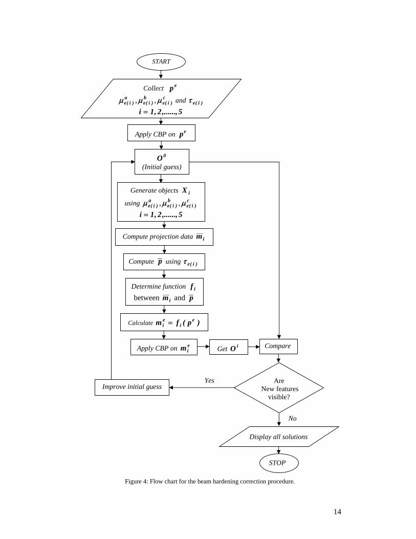
numerical algorithm described here is summarized in the flow chart of Figure 4. 4. RESULTS AND DISCUSSION
The beam hardening correction algorithm has been tested for computer generated
objects and has been found to yield good results. A few of the test cases considered are
presented here. The numerical values of peaks in the X-ray source spectrum used in the
simulation are given in Table 1. Five different energies have been considered; the
reconstruction region is assumed to carry three different types of materials. Symbols
a)j(eμ , b
)j(eμ and c)j(eμ are the coefficients of linear attenuation for the three types
of materials namely ‘a’, ‘b’ and ‘c’ respectively at energy )j(e .
Symbols used in all the reconstructed figures and simulated objects have the
following meaning:
Min: Minimum value of the gray scale for material density
7
Max: Maximum value of the gray scale for material density
LAvg: Average value of the gray levels on the horizontal centerline
AAvg: Cross-sectionally averaged value of the gray level.
Case 1: The object considered is a circle made up of material ‘a’ with three circular
holes, one filled with material ‘b’ and two filled with material ‘c’. The number of rays
and the number of views used in calculating projection data are 128 × 128 respectively.
Figures 4, 5 and 6 shows the images obtained after applying beam hardening correction
to the experimental data of the object, at energies )1.0 ( e )1(e)1( =τ ,
)3.0 ( e )2(e)2( =τ and )2.0 ( e )4(e)4( =τ respectively. These figures can be
compared to understand the effect of change in probability )j(eτ on the
monoenergetic reconstruction of the object after the beam-hardening correction on the
projection data at that energy. All energies with different probabilities have been
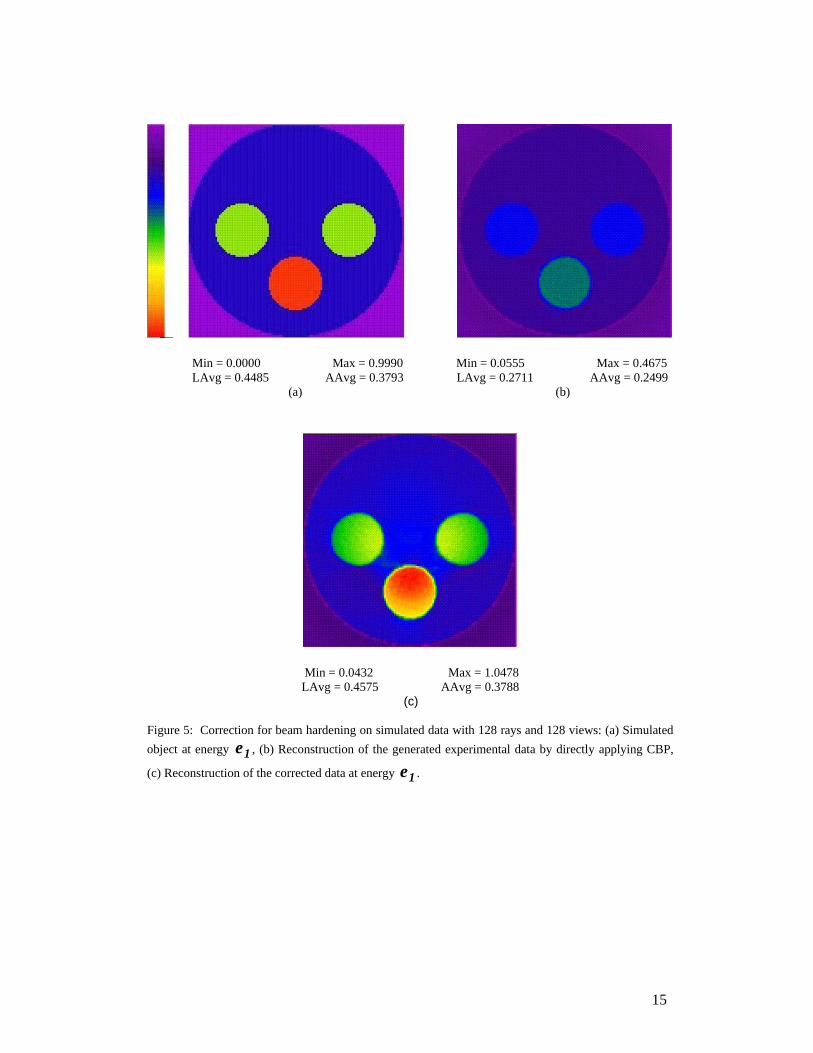
considered. Figure 5(a) is the simulated object at energy )1(e . Figure 5(b) is the
reconstruction of the experimental data by directly applying CBP to it. Figure 5(c) is
the reconstruction of the experimental data after applying beam hardening correction to
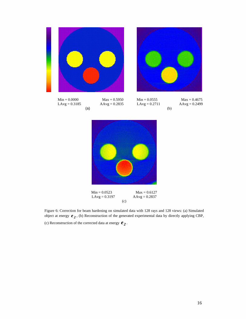
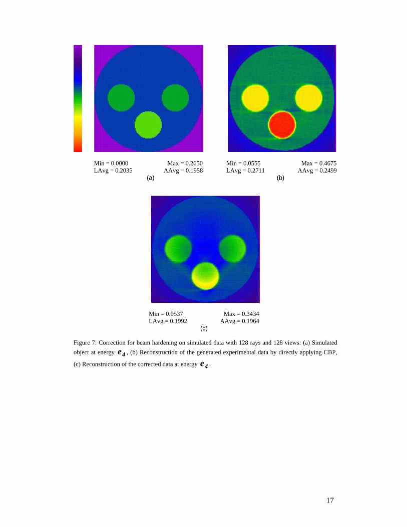
it at energy )1(e . Figure 6, at energy )2(e and Figure 7, at )4(e have the same
reconstruction procedure as given for Figure 5. Here we have considered a defect free
sample and hence we do not get any new features visible after first iteration of the
algorithm. Hence beam-hardening correction is complete after the first iteration, and its
reconstruction has been shown. From these images it is clear that beam hardening
correction will be more effective for those energies which have higher probabilities
)j(eτ . As the probability of detected photon is the least at energy )1(e , the
experimental data has least contribution from the photons of this energy. This can also
be observed from Equation (4). Hence, the experimental data does not contain much
information about the coefficient of linear attenuation of the materials in the object at
energy )1(e . This explains the non-uniform reconstruction at this energy, as shown in
the Figure 5(c). It can be observed from the figure that the reconstruction after
applying beam hardening correction at energy )2(e (which has highest probability) is
more uniform than monoenergetic reconstruction at energy )1(e and )4(e . In
principle the algorithm works for all the energies. It is recommended that beam-
8
hardening correction at the energy with the highest probability )j(eτ be used in
measurements related to NDT. Case 2: The object considered is circular in cross-section made up of material ‘a’ with
a star shaped hole inside, filled with material ‘b’. The material ‘b’ has a crack in it.
The small holes are filled with material ‘c’. Results with beam hardening correction for
this object at all the five energies has been presented in Figures 8-12. As the energy
)3(e has highest probability )j(eτ in the X-ray spectrum, the working of the
algorithm is explained here taking beam-hardening correction at energy )3(e as an
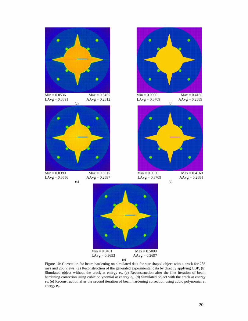
example, Figure 10. The reconstruction of the experimental data ( p ) obtained after the
X-ray tomography of the object is shown in Figure 10(a). From this reconstruction the
object type ( 0O ) can be identified. Crack is not an intrinsic property of the object; it is
present in the particular sample of the object which is defective. The object 0O is
simulated at all five energies called iX . 3X is shown in Figure 10(b). Monoenergetic
( im ) and polychromatic ( p ) projection data is calculated from iX ’s as explained
above using Equations (3) and (4) respectively. In the present discussion, the number
of rays per view are 256 and number of views are 256. Now, the function if , which
correlates p and im can be found out. Here least square curve fitting10 has been used
to get the coefficients of the polynomial function if of degree three. This function is
of the form:
33
22103 p a p a p a a m +++= (7)
The coefficients for curve fitting between p and 3m are given in Table 2. The
coefficients 0a , 1a , 2a and 3a are used to find im ’s, the monoenergetic data set for
each energy. CBP is applied to the data for all the five energies. The first
monoenergetic reconstruction at energy )3(e is shown in Figure 10(c). In the figure a
crack is clearly visible. It is a new feature as it was not present in the initial guess 0O
of the object. It is clear that the beam hardening correction should now be continued. In
the second iteration, the guessed object 1O is the one obtained from the previous
iteration. This is a star-shaped object with a crack at the location where it appeared in
9
previous monoenergetic reconstruction, Figure 10(d). The entire correction process is
repeated with 1O . The monoenergetic reconstruction after the second iteration is
shown in Figure 10(e). The coefficients of curve fitting for second iteration are given
in Table 2. We do not observe any new features in the reconstruction after second
iteration; hence the beam-hardening correction algorithm can be stopped at this stage. Case 3: Here the object is identical to case 2 with equal number of rays and views, but
the degree of polynomial curve fitting is increased to four instead of three. The
correction procedure is identical to that in Case 2. The coefficients of the curve fitting
at energy )3(e are given in Table 3. The results for this geometry are shown in Figures
13-17. Comparing the results of case 2 and case 3, it can be readily inferred that the
beam hardening correction procedure leads to an improvement in the monoenergetic
reconstruction. The improvement in the reconstruction however requires more
computational power and time. In the present discussion, we have taken with 256
views and 256 rays. As this number is increased to 512 and later to 1024, the
computational time rapidly increases. Hence, for general application the third degree
polynomial curve fit is good enough for beam hardening correction. It can be increased
in principle for higher accuracy. 5. CONCLUSIONS
Correction for beam hardening is necessary in computerized tomography when the
radiation source is polyenergetic. An algorithm that can be used for this correction has
been proposed. The test objects considered consisted of three materials but the
algorithm could be used with objects that contain more than three materials as well.
For the correction of beam hardening, the spectrum of the X-ray source and the
coefficients of linear attenuation of the materials in the object at these energies are
required. This makes the computer code for beam hardening correction specific to the
radiation source and the test materials. Beam hardening correction can be done at any of the lines of the X-ray spectrum.
Results obtained in the present work show that the mean energy (which has the highest
probability of detection) is adequate. While any correlation techniques can also be used
in the algorithm, polynomial curve fitting was seen to be the least expensive, and the
results obtained were good enough for general applications. The degree of polynomial
10
need not be more than three for a good monoenergetic reconstruction. Thus the
proposed algorithm was found to be quite robust. ACKNOWLEDGEMENTS
The work reported in this paper was possible due to financial support of DRDL,
Hyderabad. Useful discussions with Dr S. Vathsal, Dr C. Muralidhar, Shri G. V. Siva
Rao and Shri S. Chakraborthy is gratefully acknowledged. REFERENCES
1. Herman G. T. (1980): Image reconstruction from projections: The fundamentals of
computerized tomography, Academic Press, New York.
2. Ramachandran G. N. and Lakshminaryanan A. V. (1970): Three- dimensional reconstruction
from radiographs and electron micrographs: Application of convolution instead of Fourier
transforms. Proc. Natl. Acad., USA, 68: 2236-240.
3. Singh Suneet, Muralidhar K. and Munshi P. (2002): Image reconstruction from incomplete-
projection data using combined ART_CBP algorithm, Defence Science Journal, 52 (3): 303-
316.
4. Natterer F. (1986): The Mathematics of the Computerized Tomography, John Wiley & Sons,
New York.
5. Manzoor M. F., Yadav P., Muralidhar K. and Munshi P. (2001): Image reconstruction of
simulated specimens using convolution back projection, Defence Science Journal, 51(2): 175-
187.
6. Development of software for image reconstruction and error analysis for Computerized
Tomography, DRDL Progress Report (Phase I), December 1999.
7. Herman G.T. (1979): Correction for Beam Hardening in Computed Tomography, Phys. Med.
Boil. 24: 81-106.
8. Herman G. T. (1979): Demonstration of Beam Hardening Correction in Computed
Tomography of the Head, J. Computed Assist. Tomography, 3: 373-378.
9. Rama Krishna K. (2000): Simulation and Correction of the Beam Hardening effect in X-ray
Tomography, M. Tech Thesis, IIT Kanpur.
10. Jain M.K., Jain R.K. and Iyengar S.R.K. (1999): Numerical methods for Scientific and
Engineering Computation, New Age International [P] Ltd., 3rd Edition.
11
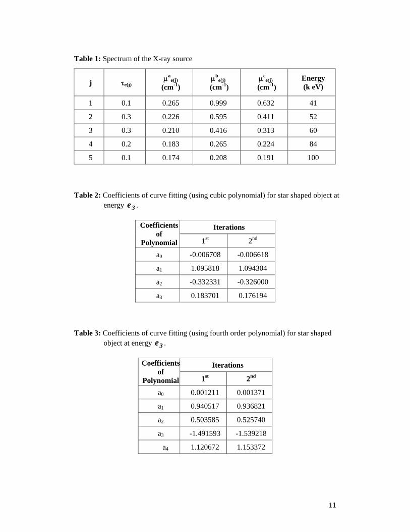
Table 1: Spectrum of the X-ray source
Table 2: Coefficients of curve fitting (using cubic polynomial) for star shaped object at
energy 3e .
Iterations Coefficientsof
Polynomial 1st 2nd
a0 -0.006708 -0.006618
a1 1.095818 1.094304
a2 -0.332331 -0.326000
a3 0.183701 0.176194 Table 3: Coefficients of curve fitting (using fourth order polynomial) for star shaped
object at energy 3e .
Iterations Coefficientsof
Polynomial 1st 2nd
a0 0.001211 0.001371
a1 0.940517 0.936821
a2 0.503585 0.525740
a3 -1.491593 -1.539218
a4 1.120672 1.153372
j τe(j) μa
e(j) (cm-1)
μbe(j)
(cm-1) μc
e(j) (cm-1)
Energy (k eV)
1 0.1 0.265 0.999 0.632 41
2 0.3 0.226 0.595 0.411 52
3 0.3 0.210 0.416 0.313 60
4 0.2 0.183 0.265 0.224 84
5 0.1 0.174 0.208 0.191 100
12
Figure 1: Parallel beam geometry for the collection of projection data
X-Ray Spectrum for Tungsten
0
500
1000
1500
2000
2500
0 15 30 45 60 75
Energy (in Kev)
Phot
on C
ount
s
Figure 2: A typical X-ray energy spectrum for tungsten.
13
Min = 0.0925 Max = 0.6775 LAvg = 0.3397 AAvg = 0.4922
(a)
Min = 0.0000 Max = 0.4160 LAvg = 0.2594 AAvg = 0.3531
(b)
Figure 3: Reconstructed star shaped object of a two-density material: (a) without the application of beam hardening correction (b) after the application of beam hardening corrections. Note that in (b), the small circles are well-resolved.
14
Figure 4: Flow chart for the beam hardening correction procedure.
Collect ep
a)i(eμ , b
)i(eμ , c)i(eμ and )i(eτ
5,......,2 ,1i =
Apply CBP on ep
0O (Initial guess)
START
Get iO
Are New features
visible?Improve initial guess
Yes
No
STOP
Compute projection data im
Compute p using )i(eτ
Generate objects iX
using a)i(eμ , b
)i(eμ , c)i(eμ
5 ,......,2 ,1i =
Determine function if between im and p
Calculate )p(fm ei
ei =
Apply CBP on eim Compare
Display all solutions
15
Min = 0.0000 Max = 0.9990 Min = 0.0555 Max = 0.4675
LAvg = 0.4485 AAvg = 0.3793 LAvg = 0.2711 AAvg = 0.2499 (a) (b)
Min = 0.0432 Max = 1.0478 LAvg = 0.4575 AAvg = 0.3788 (c) Figure 5: Correction for beam hardening on simulated data with 128 rays and 128 views: (a) Simulated object at energy 1e , (b) Reconstruction of the generated experimental data by directly applying CBP,
(c) Reconstruction of the corrected data at energy 1e .
16
Min = 0.0000 Max = 0.5950 Min = 0.0555 Max = 0.4675 LAvg = 0.3185 AAvg = 0.2835 LAvg = 0.2711 AAvg = 0.2499
(a) (b)
Min = 0.0523 Max = 0.6127 LAvg = 0.3197 AAvg = 0.2837
(c) Figure 6: Correction for beam hardening on simulated data with 128 rays and 128 views: (a) Simulated object at energy 2e , (b) Reconstruction of the generated experimental data by directly applying CBP,
(c) Reconstruction of the corrected data at energy 2e .
17
Min = 0.0000 Max = 0.2650 Min = 0.0555 Max = 0.4675 LAvg = 0.2035 AAvg = 0.1958 LAvg = 0.2711 AAvg = 0.2499 (a) (b)
Min = 0.0537 Max = 0.3434 LAvg = 0.1992 AAvg = 0.1964
(c) Figure 7: Correction for beam hardening on simulated data with 128 rays and 128 views: (a) Simulated object at energy 4e , (b) Reconstruction of the generated experimental data by directly applying CBP,
(c) Reconstruction of the corrected data at energy 4e .
18
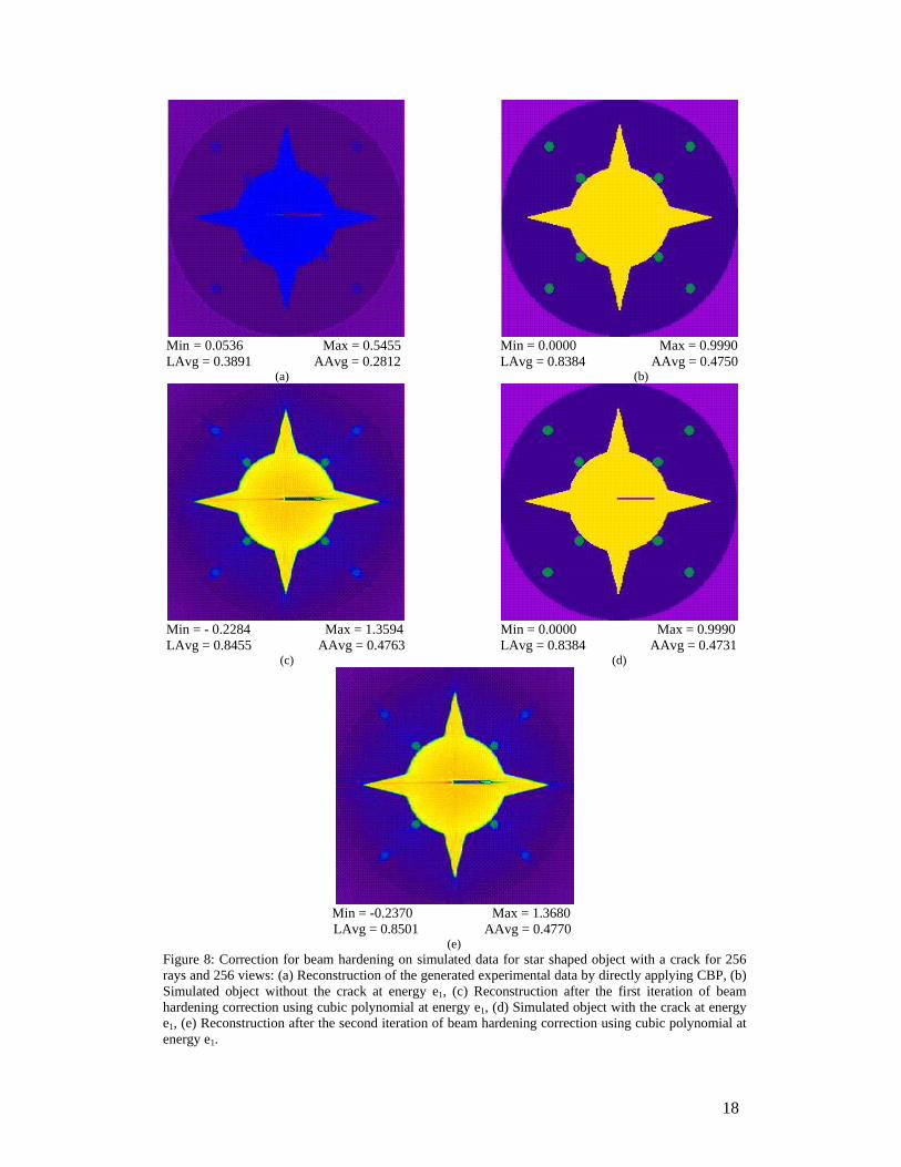
Min = 0.0536 Max = 0.5455 Min = 0.0000 Max = 0.9990 LAvg = 0.3891 AAvg = 0.2812 LAvg = 0.8384 AAvg = 0.4750 (a) (b)
Min = - 0.2284 Max = 1.3594 Min = 0.0000 Max = 0.9990 LAvg = 0.8455 AAvg = 0.4763 LAvg = 0.8384 AAvg = 0.4731 (c) (d)
Min = -0.2370 Max = 1.3680 LAvg = 0.8501 AAvg = 0.4770 (e) Figure 8: Correction for beam hardening on simulated data for star shaped object with a crack for 256 rays and 256 views: (a) Reconstruction of the generated experimental data by directly applying CBP, (b) Simulated object without the crack at energy e1, (c) Reconstruction after the first iteration of beam hardening correction using cubic polynomial at energy e1, (d) Simulated object with the crack at energy e1, (e) Reconstruction after the second iteration of beam hardening correction using cubic polynomial at energy e1.
19
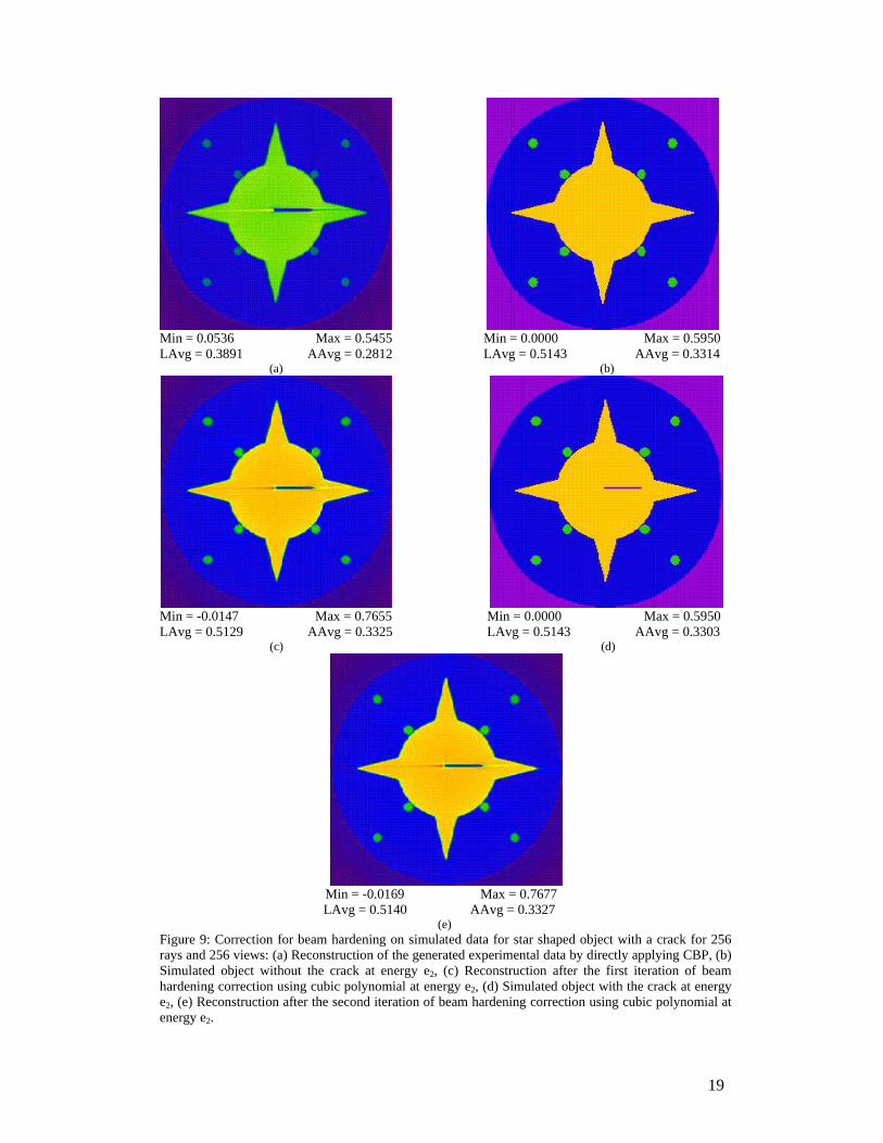
Min = 0.0536 Max = 0.5455 Min = 0.0000 Max = 0.5950 LAvg = 0.3891 AAvg = 0.2812 LAvg = 0.5143 AAvg = 0.3314 (a) (b)
Min = -0.0147 Max = 0.7655 Min = 0.0000 Max = 0.5950 LAvg = 0.5129 AAvg = 0.3325 LAvg = 0.5143 AAvg = 0.3303 (c) (d)
Min = -0.0169 Max = 0.7677 LAvg = 0.5140 AAvg = 0.3327 (e) Figure 9: Correction for beam hardening on simulated data for star shaped object with a crack for 256 rays and 256 views: (a) Reconstruction of the generated experimental data by directly applying CBP, (b) Simulated object without the crack at energy e2, (c) Reconstruction after the first iteration of beam hardening correction using cubic polynomial at energy e2, (d) Simulated object with the crack at energy e2, (e) Reconstruction after the second iteration of beam hardening correction using cubic polynomial at energy e2.
20
Min = 0.0536 Max = 0.5455 Min = 0.0000 Max = 0.4160 LAvg = 0.3891 AAvg = 0.2812 LAvg = 0.3709 AAvg = 0.2689 (a) (b)
Min = 0.0399 Max = 0.5015 Min = 0.0000 Max = 0.4160 LAvg = 0.3656 AAvg = 0.2697 LAvg = 0.3709 AAvg = 0.2681 (c) (d)
Min = 0.0401 Max = 0.5009 LAvg = 0.3653 AAvg = 0.2697 (e) Figure 10: Correction for beam hardening on simulated data for star shaped object with a crack for 256 rays and 256 views: (a) Reconstruction of the generated experimental data by directly applying CBP, (b) Simulated object without the crack at energy e3, (c) Reconstruction after the first iteration of beam hardening correction using cubic polynomial at energy e3, (d) Simulated object with the crack at energy e3, (e) Reconstruction after the second iteration of beam hardening correction using cubic polynomial at energy e3.
21
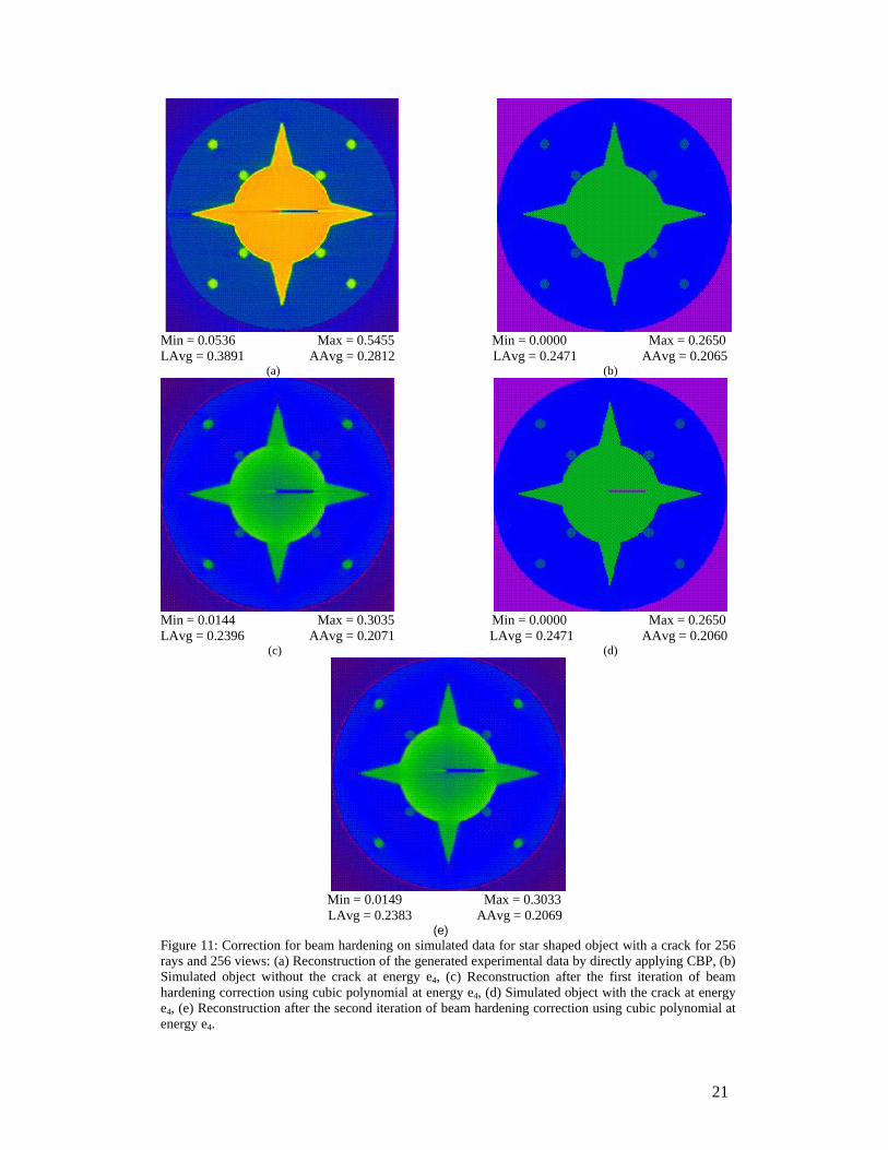
Min = 0.0536 Max = 0.5455 Min = 0.0000 Max = 0.2650 LAvg = 0.3891 AAvg = 0.2812 LAvg = 0.2471 AAvg = 0.2065 (a) (b)
Min = 0.0144 Max = 0.3035 Min = 0.0000 Max = 0.2650 LAvg = 0.2396 AAvg = 0.2071 LAvg = 0.2471 AAvg = 0.2060
(c) (d)
Min = 0.0149 Max = 0.3033 LAvg = 0.2383 AAvg = 0.2069 (e) Figure 11: Correction for beam hardening on simulated data for star shaped object with a crack for 256 rays and 256 views: (a) Reconstruction of the generated experimental data by directly applying CBP, (b) Simulated object without the crack at energy e4, (c) Reconstruction after the first iteration of beam hardening correction using cubic polynomial at energy e4, (d) Simulated object with the crack at energy e4, (e) Reconstruction after the second iteration of beam hardening correction using cubic polynomial at energy e4.
22
Min = 0.0536 Max = 0.5455 Min = 0.0000 Max = 0.2080 LAvg = 0.3891 AAvg = 0.2812 LAvg = 0.2006 AAvg = 0.1837 (a) (b)
Min = 0.0045 Max = 0.2564 Min = 0.0000 Max = 0.2080 LAvg = 0.1922 AAvg = 0.1843 LAvg = 0.2006 AAvg = 0.1833
(c) (d)
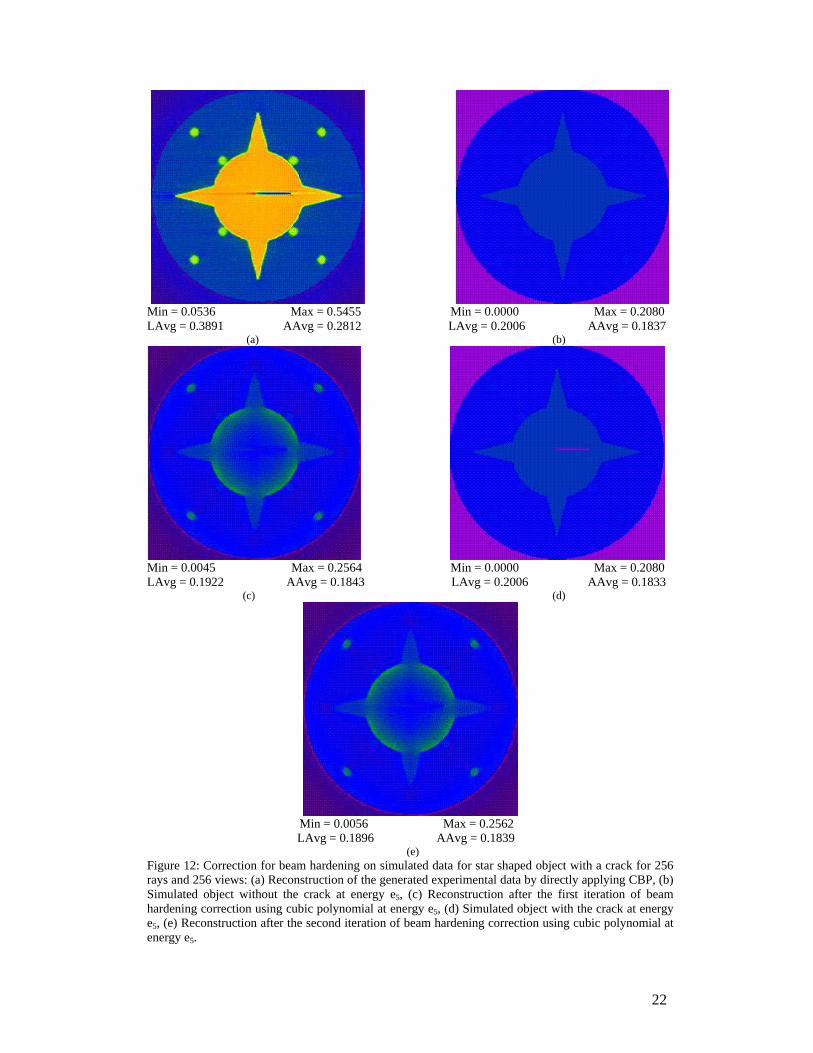
Min = 0.0056 Max = 0.2562 LAvg = 0.1896 AAvg = 0.1839 (e) Figure 12: Correction for beam hardening on simulated data for star shaped object with a crack for 256 rays and 256 views: (a) Reconstruction of the generated experimental data by directly applying CBP, (b) Simulated object without the crack at energy e5, (c) Reconstruction after the first iteration of beam hardening correction using cubic polynomial at energy e5, (d) Simulated object with the crack at energy e5, (e) Reconstruction after the second iteration of beam hardening correction using cubic polynomial at energy e5.
23
Min = 0.0536 Max = 0.5455 Min = 0.0000 Max = 0.9990 LAvg = 0.3891 AAvg = 0.2812 LAvg = 0.8384 AAvg = 0.4750 (a) (b)
Min = -0.1191 Max = 1.3355 Min = 0.0000 Max = 0.9990 LAvg = 0.8079 AAvg = 0.4742 LAvg = 0.8384 AAvg = 0.4731 (c) (d)
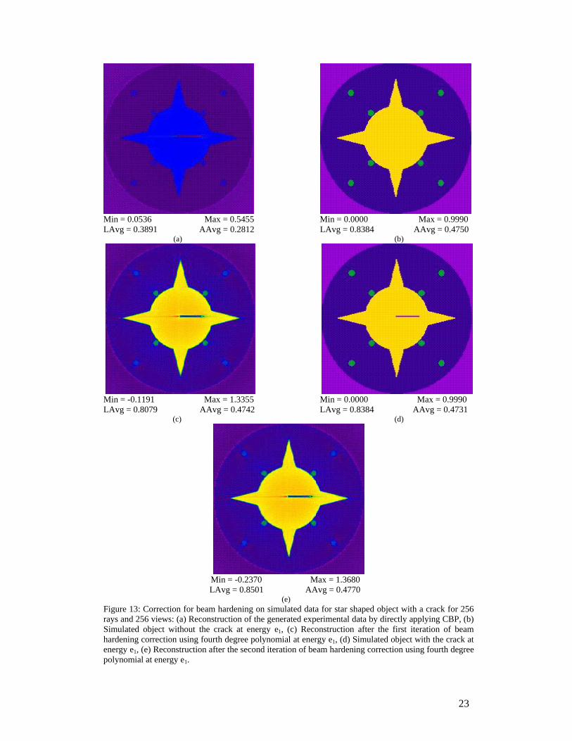
Min = -0.2370 Max = 1.3680 LAvg = 0.8501 AAvg = 0.4770 (e) Figure 13: Correction for beam hardening on simulated data for star shaped object with a crack for 256 rays and 256 views: (a) Reconstruction of the generated experimental data by directly applying CBP, (b) Simulated object without the crack at energy e1, (c) Reconstruction after the first iteration of beam hardening correction using fourth degree polynomial at energy e1, (d) Simulated object with the crack at energy e1, (e) Reconstruction after the second iteration of beam hardening correction using fourth degree polynomial at energy e1.
24
Min = 0.0536 Max = 0.5455 Min = 0.0000 Max = 0.5950 LAvg = 0.3891 AAvg = 0.2812 LAvg = 0.5143 AAvg = 0.3314 (a) (b)
Min = 0.0084 Max = 0.7604 Min = 0.0000 Max = 0.5950 LAvg = 0.5049 AAvg = 0.3321 LAvg = 0.5143 AAvg = 0.3303 (c) (d)
Min = -0.0169 Max = 0.7677
LAvg = 0.5140 AAvg = 0.3327 (e)
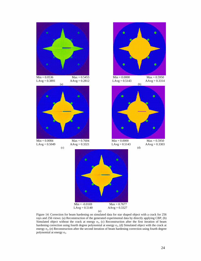
Figure 14: Correction for beam hardening on simulated data for star shaped object with a crack for 256 rays and 256 views: (a) Reconstruction of the generated experimental data by directly applying CBP, (b) Simulated object without the crack at energy e2, (c) Reconstruction after the first iteration of beam hardening correction using fourth degree polynomial at energy e2, (d) Simulated object with the crack at energy e2, (e) Reconstruction after the second iteration of beam hardening correction using fourth degree polynomial at energy e2.
25
Min = 0.0536 Max = 0.5455 Min = 0.0000 Max = 0.4160 LAvg = 0.3891 AAvg = 0.2812 LAvg = 0.3709 AAvg = 0.2689 (a) (b)
Min = 0.0553 Max = 0.5051 Min = 0.0000 Max = 0.4160 LAvg = 0.3711 AAvg = 0.2700 LAvg = 0.3709 AAvg = 0.2681 (c) (d)
Min = 0.0556 Max = 0.5049 LAvg = 0.3712 AAvg = 0.2700
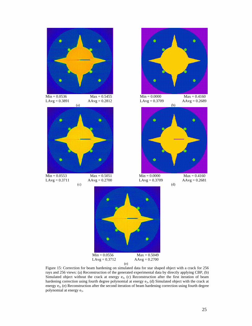
(e) Figure 15: Correction for beam hardening on simulated data for star shaped object with a crack for 256 rays and 256 views: (a) Reconstruction of the generated experimental data by directly applying CBP, (b) Simulated object without the crack at energy e3, (c) Reconstruction after the first iteration of beam hardening correction using fourth degree polynomial at energy e3, (d) Simulated object with the crack at energy e3, (e) Reconstruction after the second iteration of beam hardening correction using fourth degree polynomial at energy e3.
26
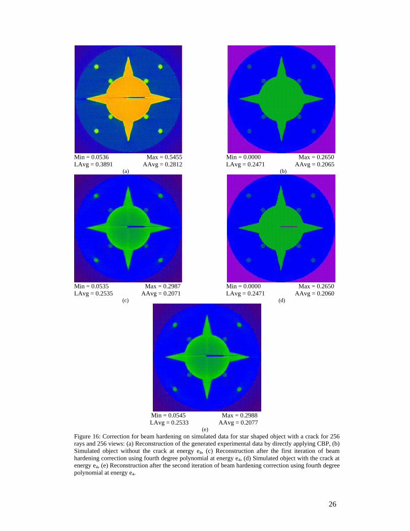
Min = 0.0536 Max = 0.5455 Min = 0.0000 Max = 0.2650 LAvg = 0.3891 AAvg = 0.2812 LAvg = 0.2471 AAvg = 0.2065
(a) (b)
Min = 0.0535 Max = 0.2987 Min = 0.0000 Max = 0.2650 LAvg = 0.2535 AAvg = 0.2071 LAvg = 0.2471 AAvg = 0.2060 (c) (d)
Min = 0.0545 Max = 0.2988 LAvg = 0.2533 AAvg = 0.2077 (e) Figure 16: Correction for beam hardening on simulated data for star shaped object with a crack for 256 rays and 256 views: (a) Reconstruction of the generated experimental data by directly applying CBP, (b) Simulated object without the crack at energy e4, (c) Reconstruction after the first iteration of beam hardening correction using fourth degree polynomial at energy e4, (d) Simulated object with the crack at energy e4, (e) Reconstruction after the second iteration of beam hardening correction using fourth degree polynomial at energy e4.
27
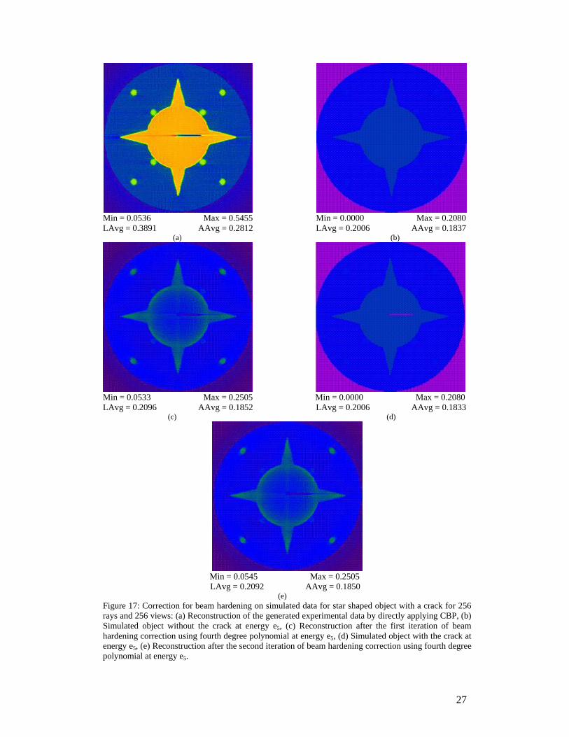
Min = 0.0536 Max = 0.5455 Min = 0.0000 Max = 0.2080 LAvg = 0.3891 AAvg = 0.2812 LAvg = 0.2006 AAvg = 0.1837 (a) (b)
Min = 0.0533 Max = 0.2505 Min = 0.0000 Max = 0.2080 LAvg = 0.2096 AAvg = 0.1852 LAvg = 0.2006 AAvg = 0.1833 (c) (d)
Min = 0.0545 Max = 0.2505 LAvg = 0.2092 AAvg = 0.1850 (e) Figure 17: Correction for beam hardening on simulated data for star shaped object with a crack for 256 rays and 256 views: (a) Reconstruction of the generated experimental data by directly applying CBP, (b) Simulated object without the crack at energy e5, (c) Reconstruction after the first iteration of beam hardening correction using fourth degree polynomial at energy e5, (d) Simulated object with the crack at energy e5, (e) Reconstruction after the second iteration of beam hardening correction using fourth degree polynomial at energy e5.