Embed Size (px)
Citation preview
www.elsevier.com/locate/atmos
Atmospheric Research 72 (2004) 263–289
An algorithm for generating stochastic cloud fields
from radar profile statistics$
K. Franklin Evansa,*, Warren J. Wiscombeb
aProgram in Atmospheric and Oceanic Sciences, University of Colorado, Boulder, CO 80309-0311, USAbLaboratory for Atmospheres, Climate and Radiation Branch, NASA Goddard Space Flight Center,
Greenbelt, MD 20771, USA
Received 31 July 2003; received in revised form 22 December 2003; accepted 31 March 2004
Abstract
An algorithm is described for generating stochastic three-dimensional (3D) cloud fields from
time–height fields derived from vertically pointing radar. This model is designed to generate cloud
fields that match the statistics of the input fields as closely as possible. The major assumptions of the
algorithm are that the statistics of the fields are translationally invariant in the horizontal and
independent of horizontal direction; however, the statistics do depend on height. The algorithm
outputs 2D or 3D stochastic fields of liquid water content (LWC) and (optionally) effective radius.
The algorithm is a generalization of the Fourier filtering methods often used for stochastic cloud
models. The Fourier filtering procedure generates Gaussian stochastic fields from a ‘‘Gaussian’’
cross-correlation matrix, which is a function of a pair of heights and the horizontal distance (or
‘‘lag’’). The Gaussian fields are nonlinearly transformed to give the correct LWC histogram for each
height. The ‘‘Gaussian’’ cross-correlation matrix is specially chosen so that, after the nonlinear
transformation, the cross-correlation matrix of the cloud mask fields approximately matches that
derived from the input LWC fields. The cloud mask correlation function is chosen because the clear/
cloud boundaries are thought to be important for 3D radiative transfer effects in cumulus.
The stochastic cloud generation algorithm is tested with 3 months of boundary layer cumulus
cloud data from an 8.6-mm wavelength radar on the island of Nauru. Winds from a 915-MHz wind
profiler are used to convert the radar fields from time to horizontal distance. Tests are performed
comparing the statistics of 744 radar-derived input fields to the statistics of 100 2D and 3D stochastic
output fields. The single-point statistics as a function of height agree nearly perfectly. The input and
stochastic cloud mask cross-correlation matrices agree fairly well. The cloud fractions agree to
within 0.005 (the total cloud fraction is 18%). The cumulative distributions of optical depth, cloud
thickness, cloud width, and intercloud gap length agree reasonably well. In the future, this stochastic
0169-8095/$ - see front matter D 2004 Elsevier B.V. All rights reserved.
doi:10.1016/j.atmosres.2004.03.016
$ Accepted to the Atmospheric Research special issue on Clouds and Radiation.
* Corresponding author. Fax: +1-303-492-3524.
E-mail address: [email protected] (K. Franklin Evans).
K. Franklin Evans, W.J. Wiscombe / Atmospheric Research 72 (2004) 263–289264
cloud field generation algorithm will be used to study domain-averaged 3D radiative transfer effects
in cumulus clouds.
D 2004 Elsevier B.V. All rights reserved.
Keywords: Stochastic cloud models; Tropical west Pacific; Cumulus clouds; Millimeter-wave radar
1. Introduction
The radiative effects of cloud horizontal inhomogeneity may be divided into two parts
(e.g. Cahalan et al., 1994; Varnai and Davies, 1999): (1) the one-dimensional heterogeneity
effect due to optical depth variability, and (2) the horizontal transport effect of light moving
between columns (Cahalan et al., 1994). For climate applications in which domain-
averaged fluxes are important, the first effect can be addressed adequately by the
independent column approximation, in which one-dimensional radiative transfer results
are integrated over the distribution of optical depths. There appears to be a consensus that
for overcast clouds (e.g. stratocumulus with 100% cloud fraction) the horizontal transport
effect is insignificant for domain average solar fluxes (Cahalan et al., 1994; Chambers et
al., 1997; Zuidema and Evans, 1998; Di Giuseppe and Tompkins, 2003). For broken cloud
scenes, the effect of horizontal transport on domain average solar fluxes is much more
uncertain. Studies with arrays of idealized cloud shapes (e.g. Aida, 1977; Welch and
Wielicki, 1984) indicate that there is a potential for large (more than 20%) biases from
neglecting horizontal transport. Significant horizontal transport effects have been noted in
more realistic but still idealized fields of broken clouds (Barker and Davies, 1992; Di
Giuseppe and Tompkins, 2003). Some studies of broken clouds reconstructed from remote
sensing reflectances have shown moderate but significant horizontal transport effects
(Chambers et al., 1997; O’Hirok and Gautier, 1998) while others have not, in absolute
terms (Benner and Evans, 2001). Studies with fields simulated by dynamical cloud models
have shown the horizontal transport effect to be small in the domain average even for
convective clouds (Barker et al., 1998, 1999; Fu et al., 2000; Scheirer and Macke, 2001).
Determining the significance of horizontal radiative transport in broken clouds for
climate applications requires the ability to measure and simulate the full range of actual
cloud structure. The three-dimensional (3D) cloudy radiative transfer problem is not a
radiative transfer issue, per se. Monte Carlo radiative transfer models can accurately and
efficiently model the domain average solar fluxes for arbitrary cloud fields. The difficult
issue is generating cloud property fields that are statistically representative of the cloud
fields in nature. Fields produced by dynamical cloud models are attractive because they
contain everything that is needed for radiative transfer models. However, dynamical cloud
models have not been able to simulate the realistic cloud structure needed because (1)
they are models with an unknown correspondence to reality, (2) too few cloud simulations
are used in radiative transfer studies to provide statistically meaningful results for
quantifying the significance of 3D effects in natural clouds, and (3) they have an
inadequate range of spatial scales (a 3D cloud model simulation over a GCM grid box
domain typically has 2-km grid cells, which does not resolve the radiatively relevant
cloud structure down to about 10 m).
K. Franklin Evans, W.J. Wiscombe / Atmospheric Research 72 (2004) 263–289 265
Currently, there are no techniques to measure 3D fields of cloud properties. Passive
solar and infrared remote sensing can measure the cloud top temperature and estimate the
optical depth (though with large uncertainties from 3D radiative transfer effects), but
cannot provide the complete cloud structure needed. Perhaps the most promising method
for measuring cloud structure in optically thicker clouds is millimeter-wavelength radar.
One major difficulty in using radars for retrieving cloud properties is that they measure the
sixth moment of the droplet distribution and hence are very sensitive to contamination by
precipitation. While this a serious problem, we believe that radars can provide useful cloud
structure even though microphysical retrievals are uncertain. However, cloud radars lack
the sensitivity to measure very weak cloud echos (down to � 50 dBZ or less) while
scanning rapidly enough to build up 3D structure before the cloud field changes. Two-
dimensional scanning may be feasible, but with lower sensitivity. Most cloud radars are
operated in a vertically pointing mode which allows longer time integrations for improved
sensitivity. There are several long-term monitoring projects with vertically pointing radars
including (1) the Atmospheric Radiation Measurement (ARM) program with radars in
Oklahoma, on Nauru and Manus islands in the tropical west Pacific, at Darwin in
Australia, and at Barrow in Alaska (Clothiaux et al., 1999), (2) the Chilbolton site in
England (Kilburn et al., 2000), and (3) the Cabauw Experimental Site for Atmospheric
Research (CESAR). Cloud radars have also been deployed in numerous field campaigns
(e.g. Frisch et al., 1995; Miller and Albrecht, 1995). These radars have adequate
sensitivity, vertical resolution, and time sampling to measure cloud structure. The
horizontal cloud structure information from a vertically pointing radar is somewhat
indirect, of course, since it relies on the wind advecting the clouds by the radar. It is
straightforward to convert the time dimension to distance with an advection speed to
obtain 2D (X–Z) cloud structure for radiative transfer experiments (Zuidema and Evans,
1998). However, it is likely that the horizontal transport effects of broken clouds are not
well approximated by 2D cloud structure, since 2D clouds have less side area for photon
leakage than 3D clouds. Therefore, there is a need for a numerical technique to derive
realistic 3D cloud structure from vertically pointing radar data.
The horizontal structural information from a vertically pointing radar is only statisti-
cally related to 3D cloud structure. Therefore, a method is needed to generate stochastic
cloud fields with statistics derived from radar. Since the horizontal radiative transport
effect depends on the cloud aspect ratio (e.g. Welch and Wielicki, 1984), it is important to
include vertical and horizontal structure, and their relationship, in the statistics. All
previous stochastic cloud models have attempted to generate the key aspects of realistic
cloud fields with just a few parameters. This approach is appropriate for learning how the
cloud parameters affect 3D radiative transfer, but cannot closely fit detailed measurements
of cloud structure. These simple stochastic cloud models include bounded cascade models
with internal variability (Cahalan et al., 1994; Marshak et al., 1998) and Poisson
distributions of homogeneous cloud elements (Zuev and Titov, 1995). The algorithm
developed here comes from the Fourier filtering family of stochastic cloud models (Voss,
1985, Schertzer and Lovejoy, 1988; Barker and Davies, 1992; Evans, 1993; Varnai, 2000;
Di Giuseppe and Tompkins, 2003). Usually, these models filter noise in the Fourier
domain with a power law (f k� b) to make scaling or ‘‘fractal’’ fields. The filtered
stochastic Fourier field is transformed to ‘‘real space’’, and a nonlinear function is applied
K. Franklin Evans, W.J. Wiscombe / Atmospheric Research 72 (2004) 263–289266
to each pixel to produce the cloud field (often optical depth or extinction). The attenuation
of higher Fourier frequencies by the power law introduces spatial correlations to produce
realistic looking cloud fields.
Most of the previous stochastic cloud models had no vertical variability and fixed cloud
thickness. Those with cloud top height variability tended to have uniform extinction (e.g.
Marshak et al., 1998; Varnai, 2000). Those with true 3D variability tended to have the
same statistics vertically and horizontally (e.g. Evans, 1993), though this shortcoming is
theoretically overcome in Schertzer and Lovejoy (1988). The model of Di Giuseppe and
Tompkins (2003) is different from other stochastic models in that it is based on
thermodynamical principles, but while it has a realistic vertical profile for stratocumulus,
that profile is fixed.
In contrast to previous stochastic cloud models, the approach taken here is to match the
statistics of detailed cloud structure measurements as closely as possible. This type of a
stochastic cloud algorithm could be called a data generalization model because it allows
the radar data to be generalized to three dimensions and to many realizations. The
stochastic field generation algorithm assumes that the cloud field is statistically homoge-
neous and isotropic in the horizontal (i.e. the statistics are independent of horizontal
position and the two horizontal directions are equivalent). The algorithm generates an
ensemble of liquid water content (LWC) and effective radius (re) fields (either 2D or 3D)
from input time–height images of LWC and re. The single-point probability distribution
(e.g. histogram of LWC) for each height in the output fields matches that of the radar-
derived input fields. The output fields approximately match the binary cloud mask
correlation function, B(z1, z2, x1� x2), which depends on the levels z1 and z2 and
horizontal separation x1� x2. We choose to match the two-point probability density
function of the cloud mask field because we believe that cloud boundaries are the most
relevant aspect of the field for 3D radiative transfer in broken clouds.
The next section provides an overview of the stochastic cloud field algorithm, while the
details are described in the appendix. The third section gives examples of stochastic cloud
fields generated from the ARM radar on Nauru and shows the results of tests of the
faithfulness of the stochastic cloud algorithm. The final section summarizes the paper,
discusses possible extensions to the stochastic algorithm, and its future application.
2. Stochastic cloud field generation algorithm
This section gives an overview of the stochastic field generation method and describes
the reasoning behind the choices made in developing the algorithm. The appendix gives
the full details of the algorithm. There are two fundamental assumptions that underlie the
technique: (1) the two horizontal directions are equivalent (horizontal isotropy), so that 3D
fields may be generated from statistics obtained from 2D radar-derived fields, and (2) the
statistics do not depend on horizontal location (translational invariance), but do depend on
height. It is straightforward to produce fields having the correct single-point statistics
(probability density function or pdf) for each vertical level. It is much more difficult to
generate fields having the desired two-point and higher-order statistics, which determine
the spatial structure. The general two-point probability density function assuming

K. Franklin Evans, W.J. Wiscombe / Atmospheric Research 72 (2004) 263–289 267
horizontal homogeneity and isotropy is p( q1, q2; z1, z2, x1� x2), where q1 and q2 are the
values at the points (x1, z1) and(x2, z2). Not only does this five-dimensional two-point pdf
require a huge amount of data to define it, but there do not appear to be any existing
algorithms for producing stochastic fields with that degree of generality. There are
methods, however, for generating fields with Gaussian statistics having a specified
correlation function, R(z1, z2, x1� x2). For Gaussian fields, the two-point pdf is completely
specified by the correlation function. Another reason for focussing on Gaussian fields is
that linear combinations (e.g. via Fourier transforms) of finite variance random deviates
will tend to produce Gaussian fields due to the central limit theorem.
One efficient method for generating Gaussian fields with a specified correlation function
is described here. This is a generalization of the Fourier filtering method used in previous
stochastic cloud studies. Let the cross-correlation matrix R(iz1, iz2, l) be the discrete version
of the correlation function with vertical level indices iz1 and iz2 (1V iz1, iz2VNz) and
l = ix1� ix2 the difference between horizontal indices. The first step is to Fourier transform
each iz1,iz2 element of the cross-correlation matrix from lag l to Fourier wave number k to
obtain the cross-spectral density matrix, S(iz1, iz2, k). The cross-correlation matrix must be
symmetric in l because of the horizontal isotropy assumption, so S(iz1, iz2, k) is real and
symmetric in k, and is obtained from R using a fast cosine transform. Both R and S are
symmetric in iz1, iz2. For each Fourier component k, the Nz eigenvalues, knk, and
eigenvectors, E(iz, n, k), of the cross-spectral density matrix are computed. It is in this
eigenvector/Fourier space that independent Gaussian noise is ‘‘filtered’’. In the filtering
process, zero mean, unit variance, complex Gaussian random deviates Z(n, k) are multiplied
by ‘‘filtering amplitudes’’, A(n, k). These amplitudes are the square root of the eigenvalues,
Aðn; kÞ ¼ffiffiffiffiffiffiffiffiffiffikn; k
p. The independent random components are then transformed back to ‘‘real
space’’, which produces the desired spatial correlations. The vertical transform is performed
for each k by multiplying the stochastic component vector by the eigenvector matrix,
Y ðk; izÞ ¼XNz
n¼1
Eðiz; n; kÞAðn; kÞZðn; kÞ: ð1Þ
Then Y(k, iz) is fast Fourier transformed in k to obtain there al space 2D Gaussian field,
G(ix, iz). A large ensemble of Gaussian fields generated in this manner will have the
desired cross-correlation matrix, R(iz1, iz2, l). Fig. 1 illustrates the procedure for
generating a stochastic 2D Gaussian field (and the final nonlinear transformation to a
LWC field). The appendix describes how to obtain the filtering amplitudes A(n, k) for
generating horizontally isotropic 3D Gaussian fields from the cross-correlation matrix
for 2D (X–Z) fields. This is not trivial because the azimuthally symmetric power
spectrum of planar fields ( f(x, y)) is not the same as the power spectra of lines sampled
from the planes (e.g. f(x, 0)).
The procedure described above for generating correlated stochastic Gaussian fields is
mathematically equivalent to using principal component analysis or empirical orthogonal
functions (EOFs) with random Gaussian amplitudes. Principal components are the
eigenvectors of the correlation matrix, while the eigenvalues of the correlation matrix
are the variances of each component. By construction, the principal components are
uncorrelated or orthogonal to each other. Thus stochastic principal component amplitudes
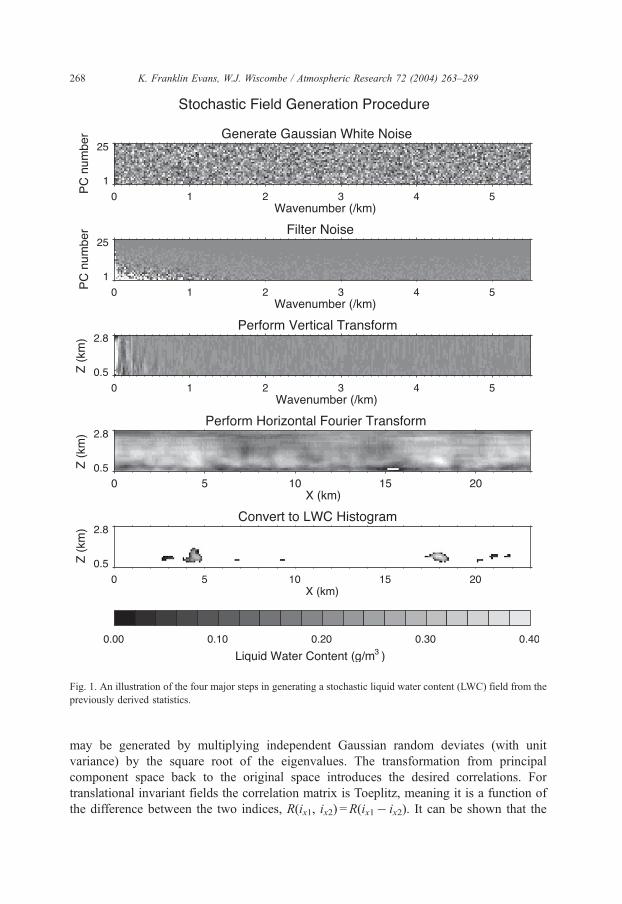
Fig. 1. An illustration of the four major steps in generating a stochastic liquid water content (LWC) field from the
previously derived statistics.
K. Franklin Evans, W.J. Wiscombe / Atmospheric Research 72 (2004) 263–289268
may be generated by multiplying independent Gaussian random deviates (with unit
variance) by the square root of the eigenvalues. The transformation from principal
component space back to the original space introduces the desired correlations. For
translational invariant fields the correlation matrix is Toeplitz, meaning it is a function of
the difference between the two indices, R(ix1, ix2) =R(ix1� ix2). It can be shown that the
K. Franklin Evans, W.J. Wiscombe / Atmospheric Research 72 (2004) 263–289 269
eigenvectors of such a correlation matrix are sines and cosines, and thus the principle
component transform is a Fourier transform. Therefore, the eigenvector/Fourier transform
procedure described above is simply a fast way to perform a principle component
transform when the statistics are translationally invariant in the horizontal.
The method described so far can generate Gaussian fields with a chosen correlation
function, but the liquid water content field of clouds is highly non-Gaussian. Not only is
the LWC distribution often similar to log-normal, but over 90% of a cumulus field has a
LWC of zero (clear sky). It is not difficult, however, to transform a Gaussian field to one
having the observed LWC pdf using a lookup table. The problem is that doing this
nonlinear transformation changes the correlation function so it no longer matches the
observed one. Therefore, we need to find the cross-correlation matrix of the Gaussian
field (‘‘Gaussian correlations’’) such that when the Gaussian field is nonlinearly
transformed, the resulting cross-correlation matrix matches the observed correlations.
The simplest method to do this would be to transform the input fields to have a
Gaussian distribution and then compute the correlation matrix. This is impossible,
however, because the huge lump of probability at zero prevents the LWC distribution
from being transformed to a smooth Gaussian distribution. Using the total water (vapor
plus cloud) content instead of LWC is a conceptually appealing way to avoid the zero
LWC problem (Di Giuseppe and Tompkins, 2003), but is not practical when deriving the
cloud statistics from measurements because the total water field is not currently
observable.
There are iterative methods that adjust the Gaussian cross-correlation matrix so that the
correct correlation function is obtained after the nonlinear transformation (e.g. Popescu et
al., 1997), but convergence is not guaranteed. Another approach is to transform the cross-
correlation matrix in LWC space to the equivalent Gaussian cross-correlation matrix. For a
given pair of levels (iz1, iz2) and horizontal distance (l), the cross-correlation matrix has
only one number to describe the two-point statistics. Thus, we have to decide what single
aspect of the full two-point pdf, p( q1, q2), is most relevant to capture. One could match the
LWC correlation, though that might be dominated by the highest LWC values. Another
choice is to match the correlation of the log of non-zero LWC values. Our interest here is
in the 3D radiative effects of cumulus fields, so we choose instead to match the cross-
correlation matrix of the binary cloud mask field, since the location of the cloud
boundaries appears to be important for finite cloud 3D radiative transfer effects. We also
note that the two-point statistics of a binary field are completely described by its
correlation function. This can be shown by considering that the two-point pdf for a binary
field reduces to four probabilities: p( q1 = 1, q2 = 1) = p12 is the probability that both points
are cloudy, p( q1 = 0, q2 = 0) is the probability that both points are clear, and p( q1 = 1,
q2 = 0) and p( q1 = 0, q2 = 1) are the probabilities one point is clear and the other is cloudy.
The four probabilities must sum to unity, and the single-point statistics provide two more
equations (related to the cloud fractions, p1 and p2, at the two points), thus there is only
one available degree of freedom in the two-point pdf. The relationship between the
correlation of the binary field (the ‘‘binary correlation’’) and the two-point probabilities
( p12, p1, p2) is given in the appendix.
The binary cross-correlation matrix is computed from the many input images. Each
input time–height LWC field is first linearly interpolated to a horizontal grid with the
K. Franklin Evans, W.J. Wiscombe / Atmospheric Research 72 (2004) 263–289270
same spacing as the vertical grid using an input aspect ratio derived from the advection
speed for that image. A user-defined threshold is then used to make the cloud mask from
the X-ZLWC field, and the cross-covariance matrix is calculated using fast Fourier
transforms. The cross-covariance matrices are accumulated and then normalized to
produce the binary field cross-correlation matrix, B(iz1, iz2, l).
The binary cross-correlation matrix is converted to the Gaussian cross-correlation
matrix element-by-element using a lookup table. The lookup table is made by numerically
integrating bivariate Gaussian distributions to relate the Gaussian space correlation to the
binary mask correlation, which also depends on the cloud fractions and hence pair of
levels, iz1, iz2. Unfortunately, the Gaussian correlation matrix produced by element-by-
element transformation is usually not positive definite, and hence some eigenvalues are
negative (i.e. negative variance). Fundamentally, this is because the elements of a
correlation matrix are not independent: if A is highly correlated with B, and B with C,
then A and C must be correlated. An optimization procedure is used to find a positive
definite correlation matrix that is close to the desired Gaussian correlation matrix. The
elements of the Cholesky decomposition of the cross-spectral density matrix S(iz1, iz2, k)
are adjusted to minimize the weighted squared error in the Gaussian correlations (with
correlations near 1 having more weight). The Cholesky decomposition H is the ‘‘square
root’’ of S (S=HHT), thus the cross-spectral density matrix is guaranteed to be positive
definite and so is the Gaussian cross-correlation matrix R(iz1, iz2, l).
The single-point statistics and the Gaussian cross-correlation matrix may be stored for
later use in generating any number of stochastic fields. The stochastic Gaussian fields
are computed as described above and then transformed to have the correct LWC
distribution with a lookup table for each vertical level. The fields in a whole ensemble,
not each output field, are forced to have the observed single-point statistics. Since the
correlation statistics used in the cloud generation algorithm are based on the cloud
boundaries, the same Gaussian correlation matrix is used to generate the effective radius
(re) fields. The Gaussian noise used to generate the re fields is correlated with the LWC
Gaussian noise so that the resulting LWC and re fields have the observed correlation.
The lookup table that converts the second set of Gaussian fields to the re fields is
derived from the input fields and depends on the LWC value. This assures that
appropriate values of re are produced for each LWC value, so that, for example,
re = 0 does not occur inside of clouds. The resulting stochastic fields should have the
correct pdf of LWC and re for each vertical level and have the observed cross-correlation
function for the binary cloud mask field. The major elements of the algorithm are
summarized in a flowchart (Fig. 2).
3. Examples and tests for cumulus fields from Nauru
The stochastic cloud field generation algorithm is tested with three months of boundary
layer cumulus cloud radar data from the ARM Millimeter-Wavelength Cloud Radar
(MMCR) on the island of Nauru (latitude 0.521jS, longitude 166.916jE). The MMCR is a
vertically pointing Doppler radar that operates at 34.86 GHz (8.6 mm) (Moran et al.,
1998). About every 40 s the MMCR cycles through four different operational modes, each
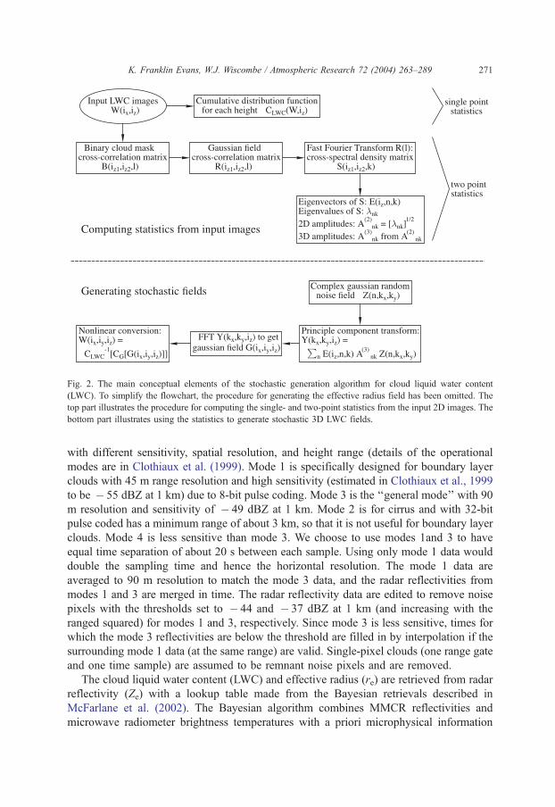
Fig. 2. The main conceptual elements of the stochastic generation algorithm for cloud liquid water content
(LWC). To simplify the flowchart, the procedure for generating the effective radius field has been omitted. The
top part illustrates the procedure for computing the single- and two-point statistics from the input 2D images. The
bottom part illustrates using the statistics to generate stochastic 3D LWC fields.
K. Franklin Evans, W.J. Wiscombe / Atmospheric Research 72 (2004) 263–289 271
with different sensitivity, spatial resolution, and height range (details of the operational
modes are in Clothiaux et al. (1999). Mode 1 is specifically designed for boundary layer
clouds with 45 m range resolution and high sensitivity (estimated in Clothiaux et al., 1999
to be � 55 dBZ at 1 km) due to 8-bit pulse coding. Mode 3 is the ‘‘general mode’’ with 90
m resolution and sensitivity of � 49 dBZ at 1 km. Mode 2 is for cirrus and with 32-bit
pulse coded has a minimum range of about 3 km, so that it is not useful for boundary layer
clouds. Mode 4 is less sensitive than mode 3. We choose to use modes 1and 3 to have
equal time separation of about 20 s between each sample. Using only mode 1 data would
double the sampling time and hence the horizontal resolution. The mode 1 data are
averaged to 90 m resolution to match the mode 3 data, and the radar reflectivities from
modes 1 and 3 are merged in time. The radar reflectivity data are edited to remove noise
pixels with the thresholds set to � 44 and � 37 dBZ at 1 km (and increasing with the
ranged squared) for modes 1 and 3, respectively. Since mode 3 is less sensitive, times for
which the mode 3 reflectivities are below the threshold are filled in by interpolation if the
surrounding mode 1 data (at the same range) are valid. Single-pixel clouds (one range gate
and one time sample) are assumed to be remnant noise pixels and are removed.
The cloud liquid water content (LWC) and effective radius (re) are retrieved from radar
reflectivity (Ze) with a lookup table made from the Bayesian retrievals described in
McFarlane et al. (2002). The Bayesian algorithm combines MMCR reflectivities and
microwave radiometer brightness temperatures with a priori microphysical information
K. Franklin Evans, W.J. Wiscombe / Atmospheric Research 72 (2004) 263–289272
from in situ cloud probes operated during shallow cumulus experiments in Hawaii and
Florida. The prior pdf of the second, third, and sixth moments of the droplet size distribution
is fitted to data from two cloud probes that measured size distributions of cloud droplets and
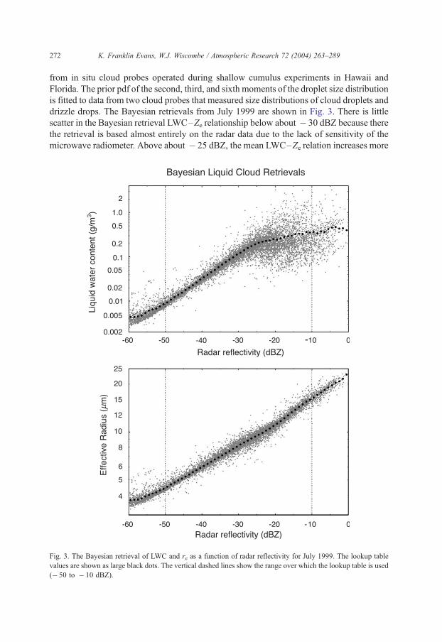
drizzle drops. The Bayesian retrievals from July 1999 are shown in Fig. 3. There is little
scatter in the Bayesian retrieval LWC–Ze relationship below about � 30 dBZ because there
the retrieval is based almost entirely on the radar data due to the lack of sensitivity of the
microwave radiometer. Above about � 25 dBZ, the mean LWC–Ze relation increases more
Fig. 3. The Bayesian retrieval of LWC and re as a function of radar reflectivity for July 1999. The lookup table
values are shown as large black dots. The vertical dashed lines show the range over which the lookup table is used
(� 50 to � 10 dBZ).
K. Franklin Evans, W.J. Wiscombe / Atmospheric Research 72 (2004) 263–289 273
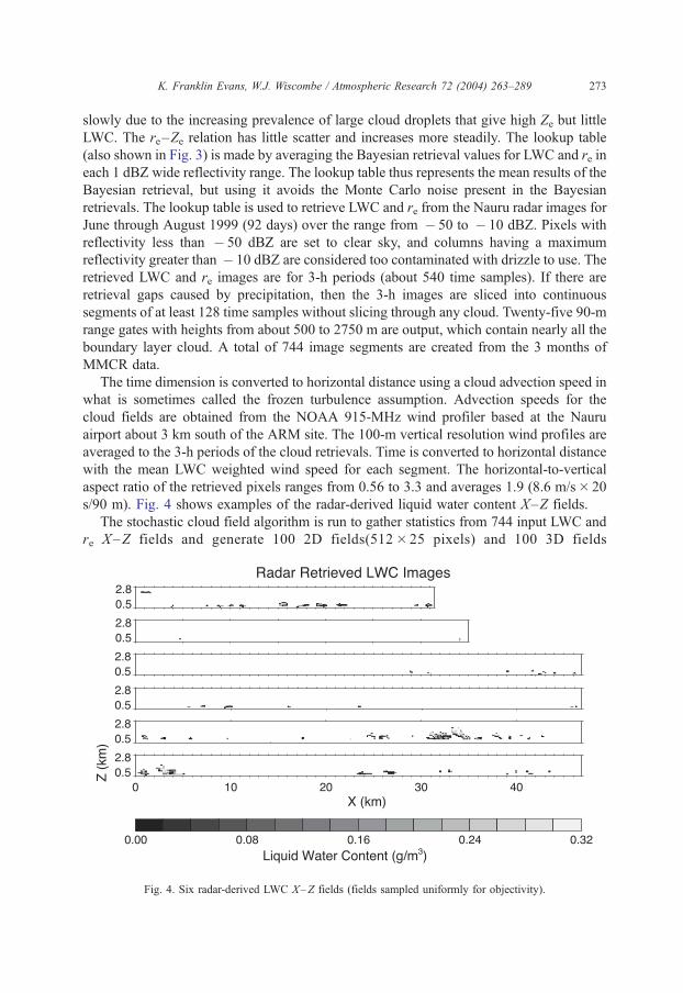
slowly due to the increasing prevalence of large cloud droplets that give high Ze but little
LWC. The re–Ze relation has little scatter and increases more steadily. The lookup table
(also shown in Fig. 3) is made by averaging the Bayesian retrieval values for LWC and re in
each 1 dBZ wide reflectivity range. The lookup table thus represents the mean results of the
Bayesian retrieval, but using it avoids the Monte Carlo noise present in the Bayesian
retrievals. The lookup table is used to retrieve LWC and re from the Nauru radar images for
June through August 1999 (92 days) over the range from � 50 to � 10 dBZ. Pixels with
reflectivity less than � 50 dBZ are set to clear sky, and columns having a maximum
reflectivity greater than � 10 dBZ are considered too contaminated with drizzle to use. The
retrieved LWC and re images are for 3-h periods (about 540 time samples). If there are
retrieval gaps caused by precipitation, then the 3-h images are sliced into continuous
segments of at least 128 time samples without slicing through any cloud. Twenty-five 90-m
range gates with heights from about 500 to 2750 m are output, which contain nearly all the
boundary layer cloud. A total of 744 image segments are created from the 3 months of
MMCR data.
The time dimension is converted to horizontal distance using a cloud advection speed in
what is sometimes called the frozen turbulence assumption. Advection speeds for the
cloud fields are obtained from the NOAA 915-MHz wind profiler based at the Nauru
airport about 3 km south of the ARM site. The 100-m vertical resolution wind profiles are
averaged to the 3-h periods of the cloud retrievals. Time is converted to horizontal distance
with the mean LWC weighted wind speed for each segment. The horizontal-to-vertical
aspect ratio of the retrieved pixels ranges from 0.56 to 3.3 and averages 1.9 (8.6 m/s� 20
s/90 m). Fig. 4 shows examples of the radar-derived liquid water content X–Z fields.
The stochastic cloud field algorithm is run to gather statistics from 744 input LWC and
re X–Z fields and generate 100 2D fields(512� 25 pixels) and 100 3D fields
Fig. 4. Six radar-derived LWC X–Z fields (fields sampled uniformly for objectivity).
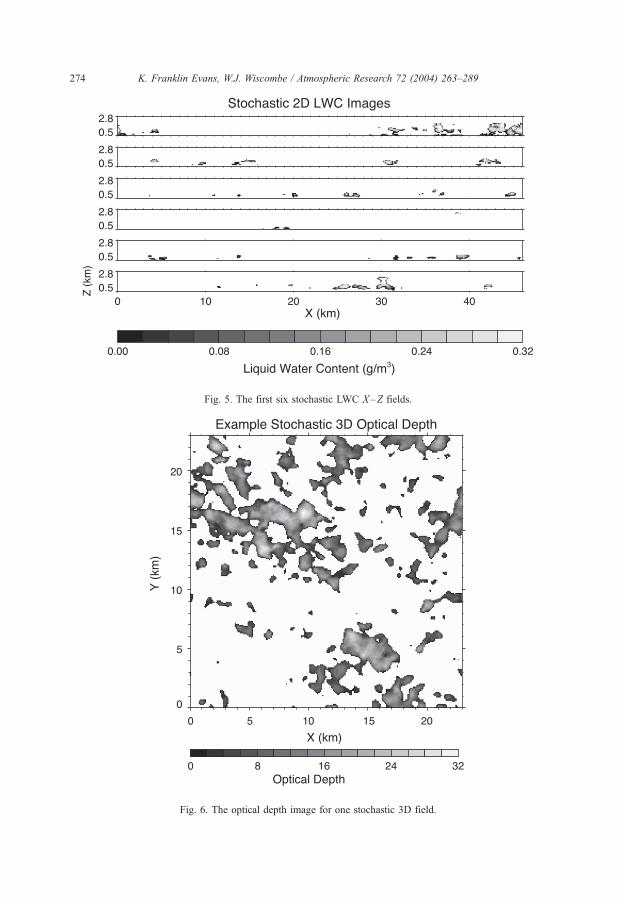
Fig. 6. The optical depth image for one stochastic 3D field.
Fig. 5. The first six stochastic LWC X–Z fields.
K. Franklin Evans, W.J. Wiscombe / Atmospheric Research 72 (2004) 263–289274
K. Franklin Evans, W.J. Wiscombe / Atmospheric Research 72 (2004) 263–289 275
(256� 256� 25pixels). The LWC threshold for making the binary cloud mask field for
the correlation matrix is 0.01 g/m3. The eigenvalue threshold kmin (see Appendix A) is
set to 10� 6 so that the eigenvalues are essentially used as is. Fig. 5 shows the first six
stochastic 2D LWC fields. The cloud fraction and peak LWC varies markedly from field
to field. The stochastic LWC fields visually show a good correspondence with the radar-
derived fields. One systematic difference that can be seen is the lack of wind sheared
clouds in the stochastic fields, since shear is an asymmetry that violates the strict
isotropy assumption made (but see Section 4 for how this problem could be remedied).
Fig. 6 shows the optical depth derived from the LWC and re of one of the 3D stochastic
fields.
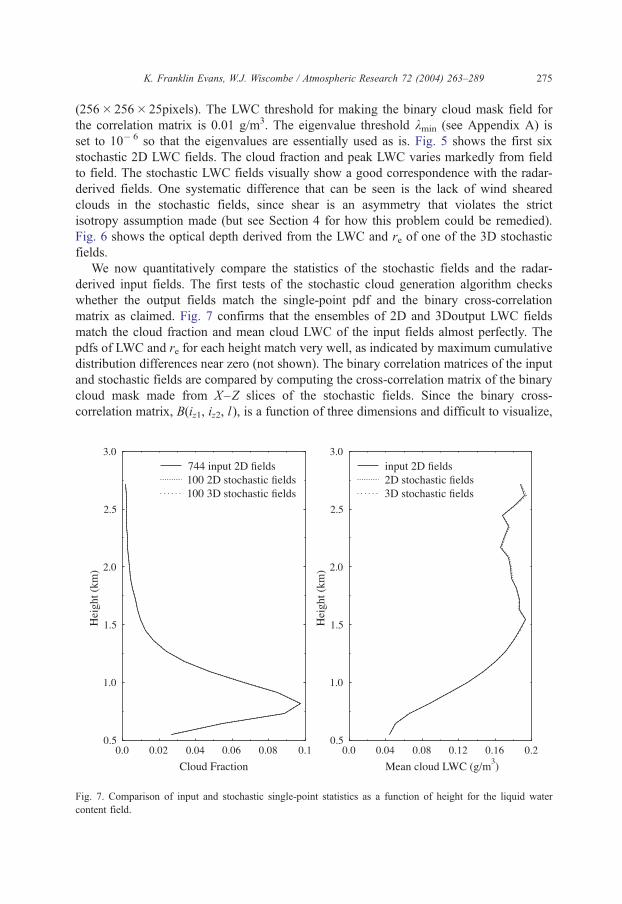
We now quantitatively compare the statistics of the stochastic fields and the radar-
derived input fields. The first tests of the stochastic cloud generation algorithm checks
whether the output fields match the single-point pdf and the binary cross-correlation
matrix as claimed. Fig. 7 confirms that the ensembles of 2D and 3Doutput LWC fields
match the cloud fraction and mean cloud LWC of the input fields almost perfectly. The
pdfs of LWC and re for each height match very well, as indicated by maximum cumulative
distribution differences near zero (not shown). The binary correlation matrices of the input
and stochastic fields are compared by computing the cross-correlation matrix of the binary
cloud mask made from X–Z slices of the stochastic fields. Since the binary cross-
correlation matrix, B(iz1, iz2, l ), is a function of three dimensions and difficult to visualize,
Fig. 7. Comparison of input and stochastic single-point statistics as a function of height for the liquid water
content field.
K. Franklin Evans, W.J. Wiscombe / Atmospheric Research 72 (2004) 263–289276
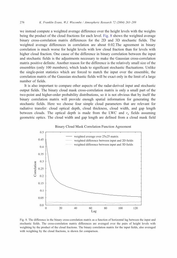
we instead compute a weighted average difference over the height levels with the weights
being the product of the cloud fractions for each level. Fig. 8 shows the weighted average
binary cross-correlation matrix differences for the 2D and 3D stochastic fields. The
weighted average differences in correlation are about 0.02.The agreement in binary
correlation is much worse for height levels with low cloud fraction than for levels with
higher cloud fraction. One cause of the difference in binary correlation between the input
and stochastic fields is the adjustments necessary to make the Gaussian cross-correlation
matrix positive definite. Another reason for the difference is the relatively small size of the
ensembles (only 100 members), which leads to significant stochastic fluctuations. Unlike
the single-point statistics which are forced to match the input over the ensemble, the
correlation matrix of the Gaussian stochastic fields will be exact only in the limit of a large
number of fields.
It is also important to compare other aspects of the radar-derived input and stochastic
output fields. The binary cloud mask cross-correlation matrix is only a small part of the
two-point and higher-order probability distributions, so it is not obvious that by itself the
binary correlation matrix will provide enough spatial information for generating the
stochastic fields. Here we choose four simple cloud parameters that are relevant for
radiative transfer: cloud optical depth, cloud thickness, cloud width, and gap length
between clouds. The optical depth is made from the LWC and re fields assuming
geometric optics. The cloud width and gap length are defined from a cloud mask field
Fig. 8. The difference in the binary cross-correlation matrix as a function of horizontal lag between the input and
stochastic fields. The cross-correlation matrix differences are averaged over the pairs of height levels with
weighting by the product of the cloud fractions. The binary correlation matrix for the input fields, also averaged
with weighting by the cloud fractions, is shown for comparison.
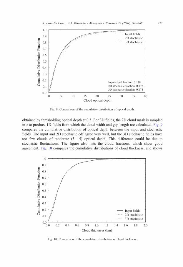
Fig. 9. Comparison of the cumulative distribution of optical depth.
K. Franklin Evans, W.J. Wiscombe / Atmospheric Research 72 (2004) 263–289 277
obtained by thresholding optical depth at 0.5. For 3D fields, the 2D cloud mask is sampled
in x to produce 1D fields from which the cloud width and gap length are calculated. Fig. 9
compares the cumulative distribution of optical depth between the input and stochastic
fields. The input and 2D stochastic cdf agree very well, but the 3D stochastic fields have
too few clouds of moderate (5–15) optical depth. This difference could be due to
stochastic fluctuations. The figure also lists the cloud fractions, which show good
agreement. Fig. 10 compares the cumulative distributions of cloud thickness, and shows
Fig. 10. Comparison of the cumulative distribution of cloud thickness.
K. Franklin Evans, W.J. Wiscombe / Atmospheric Research 72 (2004) 263–289278
the agreement to be excellent. This is not particularly surprising, since the binary cross-
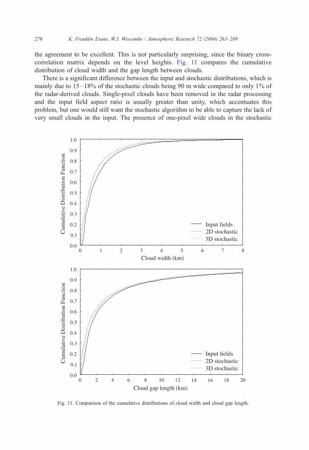
correlation matrix depends on the level heights. Fig. 11 compares the cumulative
distribution of cloud width and the gap length between clouds.
There is a significant difference between the input and stochastic distributions, which is
mainly due to 15–18% of the stochastic clouds being 90 m wide compared to only 1% of
the radar-derived clouds. Single-pixel clouds have been removed in the radar processing
and the input field aspect ratio is usually greater than unity, which accentuates this
problem, but one would still want the stochastic algorithm to be able to capture the lack of
very small clouds in the input. The presence of one-pixel wide clouds in the stochastic
Fig. 11. Comparison of the cumulative distributions of cloud width and cloud gap length.
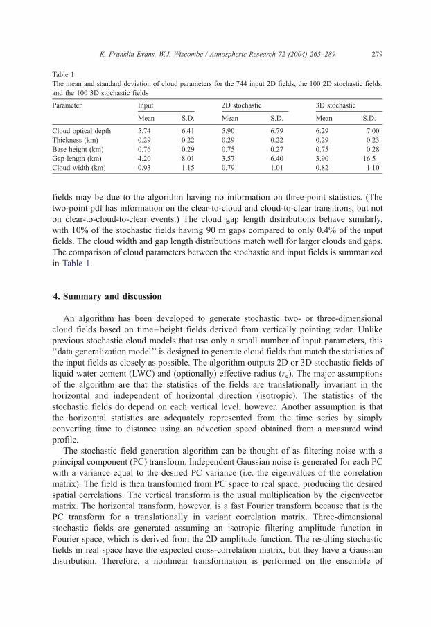
Table 1
The mean and standard deviation of cloud parameters for the 744 input 2D fields, the 100 2D stochastic fields,
and the 100 3D stochastic fields
Parameter Input 2D stochastic 3D stochastic
Mean S.D. Mean S.D. Mean S.D.
Cloud optical depth 5.74 6.41 5.90 6.79 6.29 7.00
Thickness (km) 0.29 0.22 0.29 0.22 0.29 0.23
Base height (km) 0.76 0.29 0.75 0.27 0.75 0.28
Gap length (km) 4.20 8.01 3.57 6.40 3.90 16.5
Cloud width (km) 0.93 1.15 0.79 1.01 0.82 1.10
K. Franklin Evans, W.J. Wiscombe / Atmospheric Research 72 (2004) 263–289 279
fields may be due to the algorithm having no information on three-point statistics. (The
two-point pdf has information on the clear-to-cloud and cloud-to-clear transitions, but not
on clear-to-cloud-to-clear events.) The cloud gap length distributions behave similarly,
with 10% of the stochastic fields having 90 m gaps compared to only 0.4% of the input
fields. The cloud width and gap length distributions match well for larger clouds and gaps.
The comparison of cloud parameters between the stochastic and input fields is summarized
in Table 1.
4. Summary and discussion
An algorithm has been developed to generate stochastic two- or three-dimensional
cloud fields based on time–height fields derived from vertically pointing radar. Unlike
previous stochastic cloud models that use only a small number of input parameters, this
‘‘data generalization model’’ is designed to generate cloud fields that match the statistics of
the input fields as closely as possible. The algorithm outputs 2D or 3D stochastic fields of
liquid water content (LWC) and (optionally) effective radius (re). The major assumptions
of the algorithm are that the statistics of the fields are translationally invariant in the
horizontal and independent of horizontal direction (isotropic). The statistics of the
stochastic fields do depend on each vertical level, however. Another assumption is that
the horizontal statistics are adequately represented from the time series by simply
converting time to distance using an advection speed obtained from a measured wind
profile.
The stochastic field generation algorithm can be thought of as filtering noise with a
principal component (PC) transform. Independent Gaussian noise is generated for each PC
with a variance equal to the desired PC variance (i.e. the eigenvalues of the correlation
matrix). The field is then transformed from PC space to real space, producing the desired
spatial correlations. The vertical transform is the usual multiplication by the eigenvector
matrix. The horizontal transform, however, is a fast Fourier transform because that is the
PC transform for a translationally in variant correlation matrix. Three-dimensional
stochastic fields are generated assuming an isotropic filtering amplitude function in
Fourier space, which is derived from the 2D amplitude function. The resulting stochastic
fields in real space have the expected cross-correlation matrix, but they have a Gaussian
distribution. Therefore, a nonlinear transformation is performed on the ensemble of
K. Franklin Evans, W.J. Wiscombe / Atmospheric Research 72 (2004) 263–289280
Gaussian fields so that the LWC and re single-point probability distributions match those
of the input fields at each height.
The difficult aspect of the stochastic algorithm is that the nonlinear transformation from
a Gaussian field to the LWC field changes the cross-correlation matrix. The cross-
correlation matrix is a complete description of the two-point statistics of a Gaussian field,
but not of a general field. Therefore, due to our interest in 3D radiative effects of cumulus
clouds, we choose to attempt to match the cross-correlation matrix of the cloud mask field
(as a function of two height levels and horizontal distance). With much effort, the binary
field cross-correlation matrix is translated approximately to the equivalent Gaussian field
cross-correlation matrix, so that the principal component transform method can be applied.
The algorithm is summarized in Figs. 1 and 2.
The stochastic cloud generation algorithm was tested with three months of boundary
layer cloud data (mainly trade cumulus) from the ARM radar on Nauru. A simple lookup
table is made of LWC and re from radar reflectivity using the Bayesian retrievals in
McFarlane et al. (2002). Three-hour averaged winds from the NOAA 915-MHz wind
profiler on Nauru are used to convert the radar fields from time to horizontal distance.
Tests are performed comparing the statistics of 744 radar-derived input fields to the
statistics of 100 2D and 3D stochastic output fields. The single-point statistics (e.g. cloud
fraction and mean cloud LWC) as a function of height agree nearly perfectly. The average
difference between the input and stochastic binary cloud mask cross-correlation matrices,
weighted by the product of cloud fractions, is about 0.02. The cloud fractions agree to
within 0.005 (total cloud fraction is 18%). The cumulative distribution of optical depth
agrees fairly well, while the distribution of cloud thickness agrees very well. The
stochastic algorithm produces single-pixel wide clouds even though they do not occur
in the input fields, but otherwise the distribution of cloud width and intercloud gap length
agree fairly well.
The assumptions behind the stochastic field generation algorithm could be relaxed. For
overcast clouds, it is probably not appropriate to match the cloud mask correlation
function. Instead, the algorithm could be modified to match the correlation of the log of
nonzero LWC. This can be accomplished using a lookup table made by Monte Carlo
sampling of bivariate Gaussian distributions to relate the Gaussian and log(LWC)
correlations. If one were very ambitious, the general two-point pdf might be approximated
more closely by generating a sequence of Gaussian fields with different correlation
matrices. The sequence of Gaussian fields, Gi(x, y, z), would then be combined non-
linearly, e.g. W= g(G1 + a2G22 + a3G3
3 + . . .). The difficult part, of course, is to figure out
what cross-correlation matrices to use to generate the Gaussian fields.
Even though vertically pointing radar data are the input to the algorithm, the isotropy
assumption could be relaxed. First, the anisotropic information the radar does provide, that
of upwind versus downwind, could be accommodated. This would make the correlation
function no longer symmetric in the horizontal lag. For making 3Dstochastic fields, the
correlation function could be divided into symmetric and antisymmetric parts, and the
antisymmetric part of the stochastic field could be applied with the cosine of the azimuth
angle. Second, it is possible to introduce artificial (and adjustable) anisotropy (Hinkelman,
2003). Instead of an isotropic Fourier space amplitude function, A[k], the function can be
‘‘stretched’’ in one direction (and narrowed in the other) with parameter a by substituting
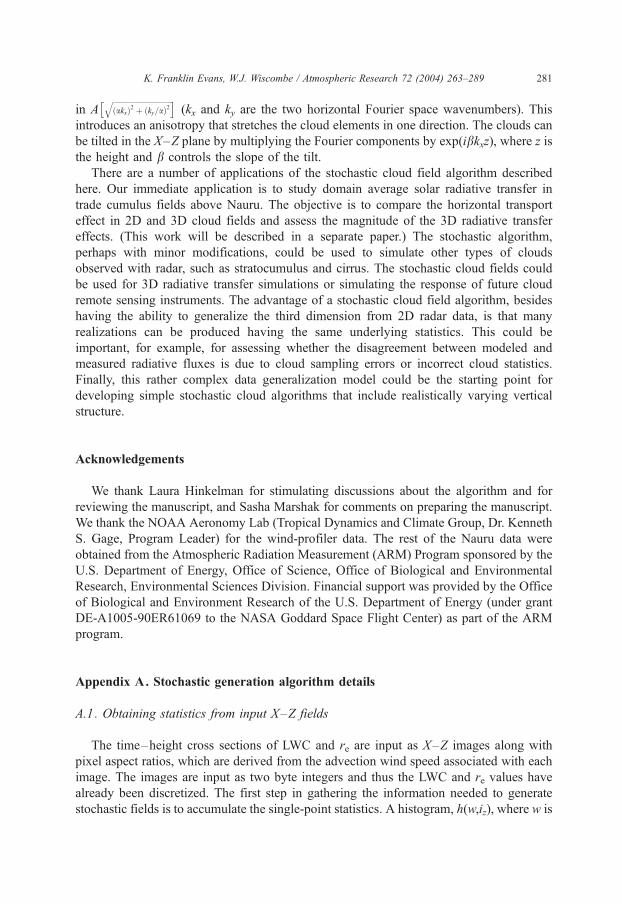
K. Franklin Evans, W.J. Wiscombe / Atmospheric Research 72 (2004) 263–289 281
in A� ffiffiffiffiffiffiffiffiffiffiffiffiffiffiffiffiffiffiffiffiffiffiffiffiffiffiffiffiffiffiffiffi
ðakxÞ2 þ ðky=aÞ2q �
(kx and ky are the two horizontal Fourier space wavenumbers). This
introduces an anisotropy that stretches the cloud elements in one direction. The clouds can
be tilted in the X–Z plane by multiplying the Fourier components by exp(ibkxz), where z isthe height and b controls the slope of the tilt.
There are a number of applications of the stochastic cloud field algorithm described
here. Our immediate application is to study domain average solar radiative transfer in
trade cumulus fields above Nauru. The objective is to compare the horizontal transport
effect in 2D and 3D cloud fields and assess the magnitude of the 3D radiative transfer
effects. (This work will be described in a separate paper.) The stochastic algorithm,
perhaps with minor modifications, could be used to simulate other types of clouds
observed with radar, such as stratocumulus and cirrus. The stochastic cloud fields could
be used for 3D radiative transfer simulations or simulating the response of future cloud
remote sensing instruments. The advantage of a stochastic cloud field algorithm, besides
having the ability to generalize the third dimension from 2D radar data, is that many
realizations can be produced having the same underlying statistics. This could be
important, for example, for assessing whether the disagreement between modeled and
measured radiative fluxes is due to cloud sampling errors or incorrect cloud statistics.
Finally, this rather complex data generalization model could be the starting point for
developing simple stochastic cloud algorithms that include realistically varying vertical
structure.
Acknowledgements
We thank Laura Hinkelman for stimulating discussions about the algorithm and for
reviewing the manuscript, and Sasha Marshak for comments on preparing the manuscript.
We thank the NOAA Aeronomy Lab (Tropical Dynamics and Climate Group, Dr. Kenneth
S. Gage, Program Leader) for the wind-profiler data. The rest of the Nauru data were
obtained from the Atmospheric Radiation Measurement (ARM) Program sponsored by the
U.S. Department of Energy, Office of Science, Office of Biological and Environmental
Research, Environmental Sciences Division. Financial support was provided by the Office
of Biological and Environment Research of the U.S. Department of Energy (under grant
DE-A1005-90ER61069 to the NASA Goddard Space Flight Center) as part of the ARM
program.
Appendix A. Stochastic generation algorithm details
A.1. Obtaining statistics from input X–Z fields
The time–height cross sections of LWC and re are input as X–Z images along with
pixel aspect ratios, which are derived from the advection wind speed associated with each
image. The images are input as two byte integers and thus the LWC and re values have
already been discretized. The first step in gathering the information needed to generate
stochastic fields is to accumulate the single-point statistics. A histogram, h(w,iz), where w is
K. Franklin Evans, W.J. Wiscombe / Atmospheric Research 72 (2004) 263–289282
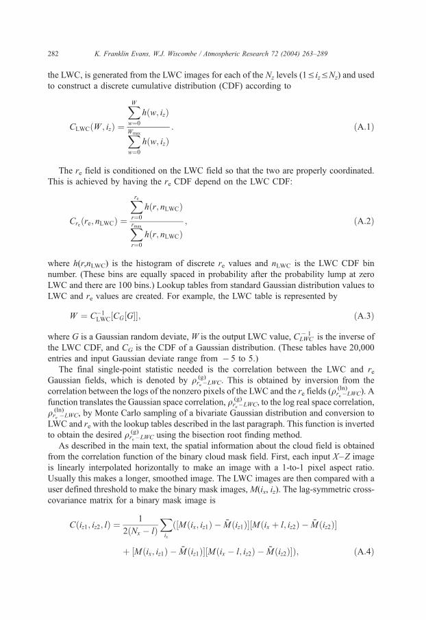
the LWC, is generated from the LWC images for each of the Nz levels (1V izVNz) and used
to construct a discrete cumulative distribution (CDF) according to
CLWCðW ; izÞ ¼
XWw¼0
hðw; izÞ
XWmax
w¼0
hðw; izÞ: ðA:1Þ
The re field is conditioned on the LWC field so that the two are properly coordinated.
This is achieved by having the re CDF depend on the LWC CDF:
Creðre; nLWCÞ ¼
Xrer¼0
hðr; nLWCÞ
Xrmax
r¼0
hðr; nLWCÞ; ðA:2Þ
where h(r,nLWC) is the histogram of discrete re values and nLWC is the LWC CDF bin
number. (These bins are equally spaced in probability after the probability lump at zero
LWC and there are 100 bins.) Lookup tables from standard Gaussian distribution values to
LWC and re values are created. For example, the LWC table is represented by
W ¼ C�1LWC½CG½G; ðA:3Þ
where G is a Gaussian random deviate, W is the output LWC value, CLWC� 1 is the inverse of
the LWC CDF, and CG is the CDF of a Gaussian distribution. (These tables have 20,000
entries and input Gaussian deviate range from � 5 to 5.)
The final single-point statistic needed is the correlation between the LWC and reGaussian fields, which is denoted by qre
(g)–LWC. This is obtained by inversion from the
correlation between the logs of the nonzero pixels of the LWC and the re fields (qre(ln)–LWC). A
function translates the Gaussian space correlation, qre(g)–LWC, to the log real space correlation,
qre(ln)–LWC, by Monte Carlo sampling of a bivariate Gaussian distribution and conversion to
LWC and re with the lookup tables described in the last paragraph. This function is inverted
to obtain the desired qre
(g)–LWC using the bisection root finding method.
As described in the main text, the spatial information about the cloud field is obtained
from the correlation function of the binary cloud mask field. First, each input X–Z image
is linearly interpolated horizontally to make an image with a 1-to-1 pixel aspect ratio.
Usually this makes a longer, smoothed image. The LWC images are then compared with a
user defined threshold to make the binary mask images,M(ix, iz). The lag-symmetric cross-
covariance matrix for a binary mask image is
Cðiz1; iz2; lÞ ¼1
2ðNx � lÞXix
ð½Mðix; iz1Þ � M̄ðiz1Þ½Mðix þ l; iz2Þ � M̄ðiz2Þ
þ ½Mðix; iz1Þ � M̄ðiz1Þ½Mðix � l; iz2Þ � M̄ðiz2ÞÞ; ðA:4Þ
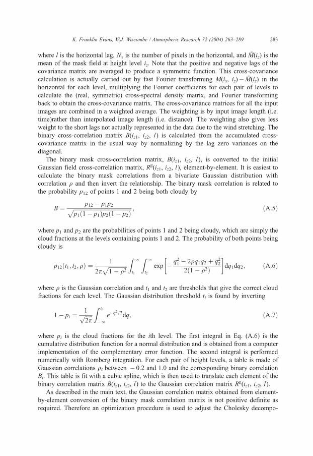
K. Franklin Evans, W.J. Wiscombe / Atmospheric Research 72 (2004) 263–289 283
where l is the horizontal lag, Nx is the number of pixels in the horizontal, and M̄(iz) is the
mean of the mask field at height level iz. Note that the positive and negative lags of the
covariance matrix are averaged to produce a symmetric function. This cross-covariance
calculation is actually carried out by fast Fourier transforming M(ix, iz)� M̄(iz) in the
horizontal for each level, multiplying the Fourier coefficients for each pair of levels to
calculate the (real, symmetric) cross-spectral density matrix, and Fourier transforming
back to obtain the cross-covariance matrix. The cross-covariance matrices for all the input
images are combined in a weighted average. The weighting is by input image length (i.e.
time)rather than interpolated image length (i.e. distance). The weighting also gives less
weight to the short lags not actually represented in the data due to the wind stretching. The
binary cross-correlation matrix B(iz1, iz2, l ) is calculated from the accumulated cross-
covariance matrix in the usual way by normalizing by the lag zero variances on the
diagonal.
The binary mask cross-correlation matrix, B(iz1, iz2, l ), is converted to the initial
Gaussian field cross-correlation matrix, Rg(iz1, iz2, l ), element-by-element. It is easiest to
calculate the binary mask correlations from a bivariate Gaussian distribution with
correlation q and then invert the relationship. The binary mask correlation is related to
the probability p12 of points 1 and 2 being both cloudy by
B ¼ p12 � p1p2ffiffiffiffiffiffiffiffiffiffiffiffiffiffiffiffiffiffiffiffiffiffiffiffiffiffiffiffiffiffiffiffiffiffiffiffiffiffiffiffiffiffip1ð1� p1Þp2ð1� p2Þ
p ; ðA:5Þ
where p1 and p2 are the probabilities of points 1 and 2 being cloudy, which are simply the
cloud fractions at the levels containing points 1 and 2. The probability of both points being
cloudy is
p12ðt1; t2; qÞ ¼1
2pffiffiffiffiffiffiffiffiffiffiffiffiffi1� q2
p Z l
t1
Z l
t2
exp � q21 � 2qq1q2 þ q222ð1� q2Þ
� dq1dq2; ðA:6Þ
where q is the Gaussian correlation and t1 and t2 are thresholds that give the correct cloud
fractions for each level. The Gaussian distribution threshold ti is found by inverting
1� pi ¼1ffiffiffiffiffiffi2p
pZ ti
�le�q2=2dq; ðA:7Þ
where pi is the cloud fractions for the ith level. The first integral in Eq. (A.6) is the
cumulative distribution function for a normal distribution and is obtained from a computer
implementation of the complementary error function. The second integral is performed
numerically with Romberg integration. For each pair of height levels, a table is made of
Gaussian correlations qi between � 0.2 and 1.0 and the corresponding binary correlation
Bi. This table is fit with a cubic spline, which is then used to translate each element of the
binary correlation matrix B(iz1, iz2, l ) to the Gaussian correlation matrix Rg(iz1, iz2, l ).
As described in the main text, the Gaussian correlation matrix obtained from element-
by-element conversion of the binary mask correlation matrix is not positive definite as
required. Therefore an optimization procedure is used to adjust the Cholesky decompo-
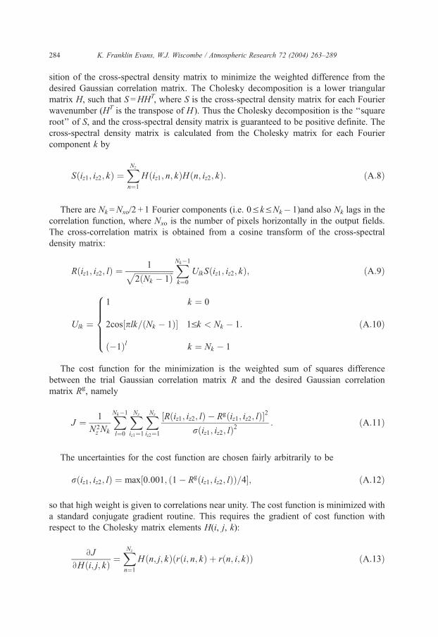
K. Franklin Evans, W.J. Wiscombe / Atmospheric Research 72 (2004) 263–289284
sition of the cross-spectral density matrix to minimize the weighted difference from the
desired Gaussian correlation matrix. The Cholesky decomposition is a lower triangular
matrix H, such that S =HHT, where S is the cross-spectral density matrix for each Fourier
wavenumber (HT is the transpose of H ). Thus the Cholesky decomposition is the ‘‘square
root’’ of S, and the cross-spectral density matrix is guaranteed to be positive definite. The
cross-spectral density matrix is calculated from the Cholesky matrix for each Fourier
component k by
Sðiz1; iz2; kÞ ¼XNz
n¼1
Hðiz1; n; kÞHðn; iz2; kÞ: ðA:8Þ
There are Nk =Nxo/2 + 1 Fourier components (i.e. 0V kVNk� 1)and also Nk lags in the
correlation function, where Nxo is the number of pixels horizontally in the output fields.
The cross-correlation matrix is obtained from a cosine transform of the cross-spectral
density matrix:
Rðiz1; iz2; lÞ ¼1ffiffiffiffiffiffiffiffiffiffiffiffiffiffiffiffiffiffiffiffi
2ðNk � 1Þp XNk�1
k¼0
UlkSðiz1; iz2; kÞ; ðA:9Þ
Ulk ¼
1 k ¼ 0
2cos½plk=ðNk � 1Þ 1Vk < Nk � 1:
ð�1Þl k ¼ Nk � 1
8>>>><>>>>:
ðA:10Þ
The cost function for the minimization is the weighted sum of squares difference
between the trial Gaussian correlation matrix R and the desired Gaussian correlation
matrix Rg, namely
J ¼ 1
N2z Nk
XNk�1
l¼0
XNz
iz1¼1
XNz
iz2¼1
½Rðiz1; iz2; lÞ � Rgðiz1; iz2; lÞ2
rðiz1; iz2; lÞ2: ðA:11Þ
The uncertainties for the cost function are chosen fairly arbitrarily to be
rðiz1; iz2; lÞ ¼ max½0:001; ð1� Rgðiz1; iz2; lÞÞ=4; ðA:12Þ
so that high weight is given to correlations near unity. The cost function is minimized with
a standard conjugate gradient routine. This requires the gradient of cost function with
respect to the Cholesky matrix elements H(i, j, k):
BJ
BHði; j; kÞ ¼XNz
n¼1
Hðn; j; kÞðrði; n; kÞ þ rðn; i; kÞÞ ðA:13Þ
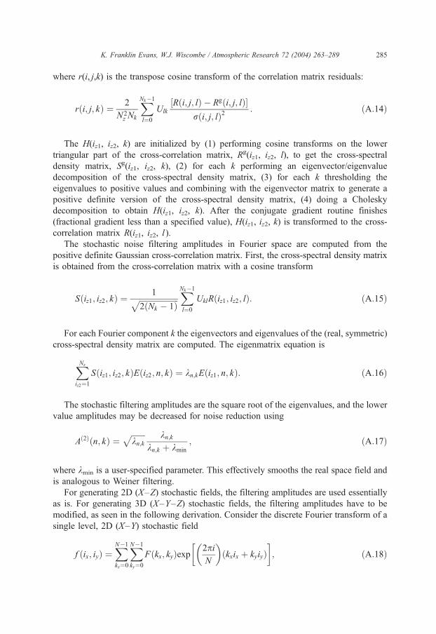
K. Franklin Evans, W.J. Wiscombe / Atmospheric Research 72 (2004) 263–289 285
where r(i, j,k) is the transpose cosine transform of the correlation matrix residuals:
rði; j; kÞ ¼ 2
N 2z Nk
XNk�1
l¼0
Ulk
½Rði; j; lÞ � Rgði; j; lÞrði; j; lÞ2
: ðA:14Þ
The H(iz1, iz2, k) are initialized by (1) performing cosine transforms on the lower
triangular part of the cross-correlation matrix, Rg(iz1, iz2, l), to get the cross-spectral
density matrix, Sg(iz1, iz2, k), (2) for each k performing an eigenvector/eigenvalue
decomposition of the cross-spectral density matrix, (3) for each k thresholding the
eigenvalues to positive values and combining with the eigenvector matrix to generate a
positive definite version of the cross-spectral density matrix, (4) doing a Cholesky
decomposition to obtain H(iz1, iz2, k). After the conjugate gradient routine finishes
(fractional gradient less than a specified value), H(iz1, iz2, k) is transformed to the cross-
correlation matrix R(iz1, iz2, l ).
The stochastic noise filtering amplitudes in Fourier space are computed from the
positive definite Gaussian cross-correlation matrix. First, the cross-spectral density matrix
is obtained from the cross-correlation matrix with a cosine transform
Sðiz1; iz2; kÞ ¼1ffiffiffiffiffiffiffiffiffiffiffiffiffiffiffiffiffiffiffiffi
2ðNk � 1Þp XNk�1
l¼0
UklRðiz1; iz2; lÞ: ðA:15Þ
For each Fourier component k the eigenvectors and eigenvalues of the (real, symmetric)
cross-spectral density matrix are computed. The eigenmatrix equation is
XNz
iz2¼1
Sðiz1; iz2; kÞEðiz2; n; kÞ ¼ kn;kEðiz1; n; kÞ: ðA:16Þ
The stochastic filtering amplitudes are the square root of the eigenvalues, and the lower
value amplitudes may be decreased for noise reduction using
Að2Þðn; kÞ ¼ffiffiffiffiffiffiffikn;k
p kn;kkn;k þ kmin
; ðA:17Þ
where kmin is a user-specified parameter. This effectively smooths the real space field and
is analogous to Weiner filtering.
For generating 2D (X–Z) stochastic fields, the filtering amplitudes are used essentially
as is. For generating 3D (X–Y–Z) stochastic fields, the filtering amplitudes have to be
modified, as seen in the following derivation. Consider the discrete Fourier transform of a
single level, 2D (X–Y) stochastic field
f ðix; iyÞ ¼XN�1
kx¼0
XN�1
ky¼0
Fðkx; kyÞexp2piN
� �ðkxix þ kyiyÞ
� ; ðA:18Þ

K. Franklin Evans, W.J. Wiscombe / Atmospheric Research 72 (2004) 263–289286
whereF(kx, ky) is the Fourier space field, f(ix, iy) is the real space field, and the fields areN�N
N�N complex numbers. The Fourier transform of a line in the X direction, f(ix, 0) (at iy= 0
for convenience), is related to the Fourier space field by
1
N
XN�1
ix¼0
f ðix; 0Þexp � 2piN
kxix
� ¼
XN�1
ky¼0
Fðkx; kyÞ: ðA:19Þ
The power spectrum for an ensemble of stochastic lines is thus
SðkxÞ ¼�����XN�1
ky¼0
Fðkx; kyÞ�����2* +
: ðA:20Þ
For isotropic stochastic fields the Fourier field is
Fðkx; kyÞ ¼ AðkÞfðkx; kyÞ; ðA:21Þ
where A(k) is the amplitude function, k ¼ffiffiffiffiffiffiffiffiffiffiffiffiffiffiffik2x þ k2y
q, and f is a field of independent
standard Gaussian random variables. Substituting in the isotropic stochastic fields gives
SðkxÞ ¼�����XN�1
ky¼0
Affiffiffiffiffiffiffiffiffiffiffiffiffiffiffik2x þ k2y
q� �fðkx; kyÞ
�����2* +
; ðA:22Þ
and, since the random variables are independent with unit variance, the power spectrum is
SðkxÞ ¼XN�1
ky¼0
Affiffiffiffiffiffiffiffiffiffiffiffiffiffiffik2x þ k2y
q� �h i2: ðA:23Þ
In this case, the power spectrum S(kx) is known from the input image statistics, but the
amplitude function A(k) is needed for the 3D stochastic field generation, and thus this
equation must be inverted. The inversion problem is turned into an optimization problem
by minimizing a cost function using a conjugate gradient routine. The cost function is
J ¼XNz
n¼1
XNk�1
kx¼0
½Sðn; kxÞ � S0ðn; kxÞ2; ðA:24Þ
where S 0(n,kx)=[A(2)(n, k)]2 is the desired power spectrum,
Sn;kx ¼XNk�1
ky¼0
cðkx; kyÞ½Að3Þðn; kÞ2; ðA:25Þ
k ¼ffiffiffiffiffiffiffiffiffiffiffiffiffiffiffik2x þ k2y
q, and c(kx,ky) = 4/[(1 + dkx,0)(1 + dky,0)]. The amplitudes for the 3D stochastic
fields, A(3)(n,k), are then found by minimizing the cost function.
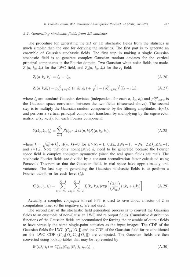
A.2. Generating stochastic fields from 2D statistics
The procedure for generating the 2D or 3D stochastic fields from the statistics is
much simpler than the one for deriving the statistics. The first part is to generate an
ensemble of Gaussian stochastic fields. The first step in making a single Gaussian
stochastic field is to generate complex Gaussian random deviates for the vertical
principal components in the Fourier domain. Two Gaussian white noise fields are made,
Z1(n, kx, ky) for the LWC field, and Z2(n, kx, ky) for the re field:
Z1ðn; kx; kyÞ ¼ f1 þ if2; ðA:26Þ
Z2ðn; kxkyÞ ¼ qðgÞre�LWCZ1ðn; kx; kyÞ þ
ffiffiffiffiffiffiffiffiffiffiffiffiffiffiffiffiffiffiffiffiffiffiffiffiffiffiffiffiffi1� ðqðgÞ
re�LWCÞ2
qðf3 þ if4Þ; ðA:27Þ
where fi are standard Gaussian deviates (independent for each n, kx, ky) and qre(g)–LWC is
the Gaussian space correlation between the two fields (discussed above). The second
step is to multiply the Gaussian random components by the filtering amplitudes, A(n,k),
and perform a vertical principal component transform by multiplying by the eigenvector
matrix, E(iz, n, k), for each Fourier component:
Yjðkx; ky; izÞ ¼XNz
n¼1
Eðiz; n; kÞAðn; kÞZjðn; kx; kyÞ; ðA:28Þ
where k ¼ffiffiffiffiffiffiffiffiffiffiffiffiffiffiffik2x þ k2y
q, A(n, k) = 0 for k >Nk� 1, 0V kxVNk� 1, �Nk+ 2V kyVNk�1,
and j = 1,2. Note that only nonnegative kx need to be generated because the Fourier
space field is complex conjugate symmetric (since the real space fields are real). The
stochastic Fourier fields are divided by a constant normalization factor calculated using
Parsevals Theorem so that the Gaussian fields in real space have approximately unit
variance. The last step in generating the Gaussian stochastic fields is to perform a
Fourier transform for each level (iz):
Gjðix; iy; izÞ ¼XNk�1
kx¼�Nkþ2
XNk�1
ky¼�Nkþ2
Yjðkx; kyizÞexp2piNxo
� �ðixkx þ iykyÞ
� : ðA:29Þ
Actually, a complex conjugate to real FFT is used to save about a factor of 2 in
computation time, so the negative kx are not used.
The second part of the stochastic field generation process is to convert the Gaussian
fields to an ensemble of non-Gaussian LWC and re output fields. Cumulative distribution
functions of the Gaussian fields are accumulated for forcing the ensemble of output fields
to have virtually the same single-point statistics as the input images. The CDF of the
Gaussian fields for LWC (CG1[G1]) and the CDF of the Gaussian field for re conditioned
on the LWC CDF (CG2[G2,CG1[G1]]) are computed. The Gaussian fields are then
converted using lookup tables that may be represented by
W ðixiy; izÞ ¼ C�1LWC ½CG1½G1ðix; iy; izÞ; ðA:30Þ
K. Franklin Evans, W.J. Wiscombe / Atmospheric Research 72 (2004) 263–289 287
K. Franklin Evans, W.J. Wiscombe / Atmospheric Research 72 (2004) 263–289288
and
rðix; iy; izÞ ¼ C�1re½CG2½G2ðix; iy; izÞ;CG1½G1ðix; iy; izÞ; ðA:31Þ
where W(ix, iy, iz) is one LWC field and r(ix, iy, iz) is one re field.
References
Aida, M.A., 1977. Scattering of solar radiation as a function of cloud dimension and orientation. J. Quant.
Spectrosc. Radiat. Transfer 17, 303–310.
Barker, H., Davies, J.A., 1992. Solar radiative fluxes for stochastic, scale-invariant broken cloud fields. J. Atmos.
Sci. 49, 1115–1126.
Barker, H.W., Morcrette, J.-J., Alexander, G.D., 1998. Broadband solar fluxes and heating rates for atmospheres
with 3D broken clouds. Quart. J. Roy. Meteor. Soc. 124, 1245–1271.
Barker, H.W., Stephens, G.L., Fu, Q., 1999. The sensitivity of domain-averaged solar fluxes to assumptions about
cloud geometry. Quart. J. Roy. Meteor. Soc. 125, 2127–2152.
Benner, T.C., Evans, K.F., 2001. Three-dimensional solar radiative transfer in small tropical cumulus fields
derived from high-resolution imagery. J. Geophys. Res. 106 (D14), 14975–14984.
Cahalan, R.F., Ridgway, W., Wiscombe, W.J., Gollmer, S., Harshvardhan, 1994. Independent pixel and Monte
Carlo estimate of stratocumulus albedo. J. Atmos. Sci. 51, 3776–3790.
Chambers, L.H., Wielicki, B.A., Evans, K.F., 1997. Independent pixel and two-dimensional estimates of Landsat-
derived cloud field albedo. J. Atmos. Sci. 54, 1525–1532.
Clothiaux, E.E., Moran, K.P., Martner, B.E., Ackerman, T.P., Mace, G.G., Uttal, T., Mather, J.H., Widener, K.B.,
Miller, M.A., Rodriguez, D.J., 1999. The atmospheric radiation measurement program cloud radars: opera-
tional modes. J. Atmos. Ocean. Technol. 16, 819–827.
Di Giuseppe, F., Tompkins, A.M., 2003. Effect of spatial organization on solar radiative transfer in three-
dimensional idealized stratocumulus cloud fields. J. Atmos. Sci. 60, 1774–1794.
Evans, K.F., 1993. A general solution for stochastic radiative transfer. Geophys. Res. Lett. 20, 2075–2078.
Frisch, A.S., Fairall, C.W., Snider, J.B., 1995. Measurement of stratus cloud and drizzle parameters in ASTEX
with a Ka-band Doppler radar and a microwave radiometer. J. Atmos. Sci. 52, 2788–2799.
Fu, Q., Cribb, M.C., Barker, H.W., Krueger, S.K., Grossman, A., 2000. Cloud geometry effects on atmospheric
solar absorption. J. Atmos. Sci. 57, 1156–1168.
Hinkelman, L.M., 2003. The effect of cumulus cloud field anisotropy on solar surface radiative fluxes and
atmospheric heating rates. PhD thesis, Pennsylvania State University, State College. 89 pp.
Kilburn, C.A.D., Chapman, D., Illingworth, A.J., Hogan, R.J., 2000. Weather observations from the Chilbolton
Advanced Meteorological Radar. Weather 55, 352–356 (Bracknell, England).
Marshak, A., Davis, A., Wiscombe, W., Ridgway, W., Cahalan, R., 1998. Biases in shortwave column absorption
in the presence of fractal clouds. J. Climate 11, 431–446.
McFarlane, S.A., Evans, K.F., Ackerman, A.S., 2002. A Bayesian algorithm for the retrieval of liquid water cloud
properties from microwave radiometer and millimeter radar data. J. Geophys. Res. 107 (D16), 4317 (DOI:
10.1029/2001JD001011).
Miller, M.A, Albrecht, B.A., 1995. Surface-based observations of mesoscale cumulus–stratocumulus interaction
during ASTEX. J. Atmos. Sci. 52, 2809–2826.
Moran, K.P., Martner, B.E., Post, M.J., Kropfli, R.A., Welsh, D.C., Widener, K.B., 1998. An unattended cloud-
profiling radar for use in climate research. Bull. Am. Meteorol. Soc. 79, 443–455.
O’Hirok, W., Gautier, C., 1998. A three-dimensional radiative transfer model to investigate the solar radiation
within a cloudy atmosphere. Part I: spatial effects. J. Atmos. Sci. 55, 2162–2179.
Popescu, R., Deodatis, G., Prevost, J.H., 1997. Simulation of homogeneous non-Gaussian stochastic vector
fields. Probab. Eng. Mech. 13, 1–13.
Schertzer, D., Lovejoy, S., 1988. Multifractal simulations and analysis of clouds by multiplicative processes.
Atmos. Res. 21, 337–361.

K. Franklin Evans, W.J. Wiscombe / Atmospheric Research 72 (2004) 263–289 289
Scheirer, R., Macke, A., 2001. On the accuracy of the independent column approximation in calculating the
downward fluxes in the UVA, UVB, and PAR spectral ranges. J. Geophys. Res. 106 (D13), 14301–14312.
Varnai, T., 2000. Influence of three-dimensional radiative effects on the spatial distribution of shortwave cloud
reflection. J. Atmos. Sci. 57, 216–229.
Varnai, T., Davies, R., 1999. Effects of cloud heterogeneities on shortwave radiation: comparison of cloud-top
variability and internal heterogeneity. J. Atmos. Sci. 56, 4206–4224.
Voss, R., 1985. Random fractal forgeries. In: Earnshaw, R.A. (Ed.), Fundamental Algorithms in Computer
Graphics. Springer-Verlag, Berlin, pp. 805–835.
Welch, R.M., Wielicki, B.A., 1984. Stratocumulus cloud field reflected fluxes: the effect of cloud shape. J. Atmos.
Sci. 41, 3085–3103.
Zuev, V.E., Titov, G.A., 1995. Radiative transfer in cloud fields with random geometry. J. Atmos. Sci. 52, 176–190.
Zuidema, P., Evans, K.F., 1998. On the validity of the independent pixel approximation for boundary layer clouds
observed during ASTEX. J. Geophys. Res. 103, 6059–6074.


![Stochastic Extended Simulation (EXSIM) of Mw 7.0 ...raiith.iith.ac.in/4119/1/Geosciences.pdfdevelopment [44] which the user can select for generating the synthetics. Comparisons with](https://img.pdfslide.net/doc/110x75/5fb30688106a31606144dbf5/stochastic-extended-simulation-exsim-of-mw-70-development-44-which-the.jpg)