AN ALGORITHM FOR THREE-DIMENSIONAL, SIMULTANEOUS MODELING OF ROOT GROWTH, TRANSIENT SOIL WATER

FLOW, AND SOLUTE TRANSPORT AND UPTAKE

Version 2.1 1997

F. Somma, V. Clausnitzer and J. W. Hopmans

ABSTRACT Somma, F., V. Clausnitzer and J. W. Hopmans, An algorithm for three-dimensional,

simultaneous modeling of root growth, transient soil water flow, and solute transport and uptake, V. 2.1, Paper no. 100034, Dept. of Land, Air, and Water Resources, U. of Calif., Davis, 1997.

A model is presented for simultaneous, dynamic simulation of soil water movement, solute transport and plant root growth. Root apices are translocated in individual growth events as a function of current local soil conditions. A three-dimensional finite-element grid over the considered soil domain serves to define the spatial distribution of soil physical properties and as framework for modeling of transient water flow and solute transport, the latter including passive and active root solute uptake, as well as zero and first-order source/sink terms. Mass balance calculations have been included for both water flow and solute transport to evaluate the performance of the numerical solution scheme. Two water extraction functions have been embodied in the model, with the possibility of taking into account osmotic potential effects on water and passive solute uptake rate. Root age effects on root water and solute uptake activity have been included, as well as the influence of nutrient deficient or eccessive concentration on root growth. Intended as a tool for testing of hypotheses on soil-plant interaction, simulations can be performed using six different levels of model complexity, depending on how much information is available. At the simplest level, root growth is simulated as a function of mechanical soil strength only. The most comprehensive level includes simulation of root and shoot growth as influenced by soil water and nutrient availability, temperature, and dynamic assimilate allocation to root and shoot.

Both the program code and this manual have been carefully inspected before printing. However, we cannot guarantee that all errors have been eliminated and would be grateful for any suggested amendments for future versions of software and manual.

The Authors.

TABLE OF CONTENTS I. INTRODUCTION ........................................................................................................................ 1 II. THEORY ..................................................................................................................................... 1 Basic Concept . . . . . . . . . . . . . . . . . . . . . . . . . . . . . . . . . . . . . . . . . . . . . . . . . . . . . . . . . . . . . 1 Soil Water Flow . . . . . . . . . . . . . . . . . . . . . . . . . . . . . . . . . . . . . . . . . . . . . . . . . . . . . . . . . . . . 3 Solute Transport . . . . . . . . . . . . . . . . . . . . . . . . . . . . . . . . . . . . . . . . . . . . . . . . . . . . . . . . . . . 4 Water and Solute Mass Balance . . . . . . . . . . . . . . . . . . . . . . . . . . . . . . . . . . . . . . . . . . . . . . . . 4 Soil Temperature . . . . . . . . . . . . . . . . . . . . . . . . . . . . . . . . . . . . . . . . . . . . . . . . . . . . . . . . . . . 5 Root Growth without Solute Transport: Level '1a' Procedure . . . . . . . . . . . . . . . . . . . . . . . . . 5 Root Growth with Solute Transport: Level '1b' Procedure . . . . . . . . . . . . . . . . . . . . . . . . . . . 7 Water Uptake: Level '2a' Procedure . . . . . . . . . . . . . . . . . . . . . . . . . . . . . . . . . . . . . . . . . . . . . 8 Solute Uptake: Level '2b' Procedure . . . . . . . . . . . . . . . . . . . . . . . . . . . . . . . . . . . . . . . . . . . . . 10 Shoot and Root Growth without Solute Transport: Level '3a' Procedure . . . . . . . . . . . . . . . . 10 Shoot and Root Growth with Solute Transport: Level '3b' Procedure . . . . . . . . . . . . . . . . . . 12 III. PREPROCESSING AND MODEL INPUT ................................................................................. 13 Creating the FEM Grid . . . . . . . . . . . . . . . . . . . . . . . . . . . . . . . . . . . . . . . . . . . . . . . . . . . . . . 13 Boundary Conditions . . . . . . . . . . . . . . . . . . . . . . . . . . . . . . . . . . . . . . . . . . . . . . . . . . . . . . . . 15 Soil Parameters . . . . . . . . . . . . . . . . . . . . . . . . . . . . . . . . . . . . . . . . . . . . . . . . . . . . . . . . . . . . 17 Solute Transport Parameters . . . . . . . . . . . . . . . . . . . . . . . . . . . . . . . . . . . . . . . . . . . . . . . . . . 17 Execution Control . . . . . . . . . . . . . . . . . . . . . . . . . . . . . . . . . . . . . . . . . . . . . . . . . . . . . . . . . . 18 Plant Growth Parameters . . . . . . . . . . . . . . . . . . . . . . . . . . . . . . . . . . . . . . . . . . . . . . . . . . . . . 19 Soil Temperature . . . . . . . . . . . . . . . . . . . . . . . . . . . . . . . . . . . . . . . . . . . . . . . . . . . . . . . . . . . 21 Root System . . . . . . . . . . . . . . . . . . . . . . . . . . . . . . . . . . . . . . . . . . . . . . . . . . . . . . . . . . . . . . . 22 IV. MODEL OUTPUT AND POSTPROCESSING .......................................................................... 27 Simulation Record . . . . . . . . . . . . . . . . . . . . . . . . . . . . . . . . . . . . . . . . . . . . . . . . . . . . . . . . . . 27 Soil Water and Solute Status . . . . . . . . . . . . . . . . . . . . . . . . . . . . . . . . . . . . . . . . . . . . . . . . . . 27 Mass Balance . . . . . . . . . . . . . . . . . . . . . . . . . . . . . . . . . . . . . . . . . . . . . . . . . . . . . . . . . . . . . 28 Root System . . . . . . . . . . . . . . . . . . . . . . . . . . . . . . . . . . . . . . . . . . . . . . . . . . . . . . . . . . . . . . . 29 V. HARDWARE AND SOFTWARE REQUIREMENTS ................................................................. 32 Using a PC . . . . . . . . . . . . . . . . . . . . . . . . . . . . . . . . . . . . . . . . . . . . . . . . . . . . . . . . . . . . . . . . 32 Portability . . . . . . . . . . . . . . . . . . . . . . . . . . . . . . . . . . . . . . . . . . . . . . . . . . . . . . . . . . . . . . . . 32 Graphics . . . . . . . . . . . . . . . . . . . . . . . . . . . . . . . . . . . . . . . . . . . . . . . . . . . . . . . . . . . . . . . . . 32 VI. PROGRAM STRUCTURE AND VARIABLES USED ............................................................... 34 Principal Design . . . . . . . . . . . . . . . . . . . . . . . . . . . . . . . . . . . . . . . . . . . . . . . . . . . . . . . . . . . 34 Program Sub-Units . . . . . . . . . . . . . . . . . . . . . . . . . . . . . . . . . . . . . . . . . . . . . . . . . . . . . . . . . . 38 Input . . . . . . . . . . . . . . . . . . . . . . . . . . . . . . . . . . . . . . . . . . . . . . . . . . . . . . . . . . . . . . . . 38 Environmental Functions . . . . . . . . . . . . . . . . . . . . . . . . . . . . . . . . . . . . . . . . . . . . . . . . . 40 Water Flow . . . . . . . . . . . . . . . . . . . . . . . . . . . . . . . . . . . . . . . . . . . . . . . . . . . . . . . . . . . 41 Sink . . . . . . . . . . . . . . . . . . . . . . . . . . . . . . . . . . . . . . . . . . . . . . . . . . . . . . . . . . . . . . . . . 44 Solute Transport . . . . . . . . . . . .. . . . . . . . . . . . . . . . . . . . . . . . . . . . . . . . . . . . . . . . . . . . 45 Plant Growth . . . . . . . . . . . . . . . . . . . . . . . . . . . . . . . . . . . . . . . . . . . . . . . . . . . . . . . . . . 47 Root Growth . . . . . . . . . . . . . . . . . . . . . . . . . . . . . . . . . . . . . . . . . . . . . . . . . . . . . . . . . . 49 Output . . . . . . . . . . . . . . . . . . . . . . . . . . . . . . . . . . . . . . . . . . . . . . . . . . . . . . . . . . . . . . . 57

REFERENCES ................................................................................................................................ 59 APPENDIX A: Numerical solution of water flow and solute transport equations ............................. 65 APPENDIX B: Variables in COMMON blocks ............................................................................... 64 APPENDIX C: Source Code Listing ................................................................................................ 77 APPENDIX D: Preprocessor Code Listing (grid.for) ....................................................................... 133 APPENDIX E: Postprocessor Code Listings (trans.for, v.for, and profile.for) ................................. 135

1

I. INTRODUCTION Previous efforts in root growth modeling have enhanced the spatial resolution of the simulated root systems to the scale of single root segments in three dimensions (Diggle, 1988; Pages et al., 1989) and considered the influence of a variety of soil environmental factors (e.g., Jones et al., 1991). The model described herein differs from previous work in that it simulates the growth of a plant root as a process controlled by the physical conditions in the soil environment while also affecting them. Individual growth and influence functions can be flexibly defined to permit the testing of hypothetical relationships. At the present stage, the objective of this study was to simulate the interactive relationships between soil water flow, solute transport, root growth and water and solute uptake processes. Given the complexity and limited current understanding of the considered processes, the model is intended as a basis for continued extension and improvement rather than for black-box-type applications. To facilitate easy access to the design of the existing code, this manual includes a section covering every subroutine and function of the current version of the program. The first version of this model simulated water flow, root growth and root water uptake (Clausnitzer and Hopmans, 1993). The present model is an extension and includes three-dimensional simulation of solute transport, including diffusion, dispersion and convection, and zero and first-order sink/source terms, with passive and active root solute uptake. The main reference for solute transport is S

vimu°nek et al. (1992).

Additional features in the present version of the model include calculation of mass balance for soil water flow and solute transport and a choice of options for calculation of the root water extraction function, with the possibility of including osmotic potential effects on water uptake rates. The root distribution function, necessary for computation of nodal water and solute sink term values, is now calculated taking into account all root segments rather than root tips only, as was done in the earlier version. Effects of root age on water and solute extraction rates, and of nutrient deficiency and toxicity on root growth have also been considered. A more thorough review and examples showing the effects of soil environmental characteristics on root growth are presented in Clausnitzer and Hopmans (1994). II. THEORY Basic Concept To make possible the simulation of dynamic interactions, a three-dimensional root growth model has been combined with a three-dimensional, transient soil water flow and solute transport model based on the finite-element method (FEM). In a preprocessing phase, the considered soil domain is discretized into a rectangular grid of finite elements with the

2

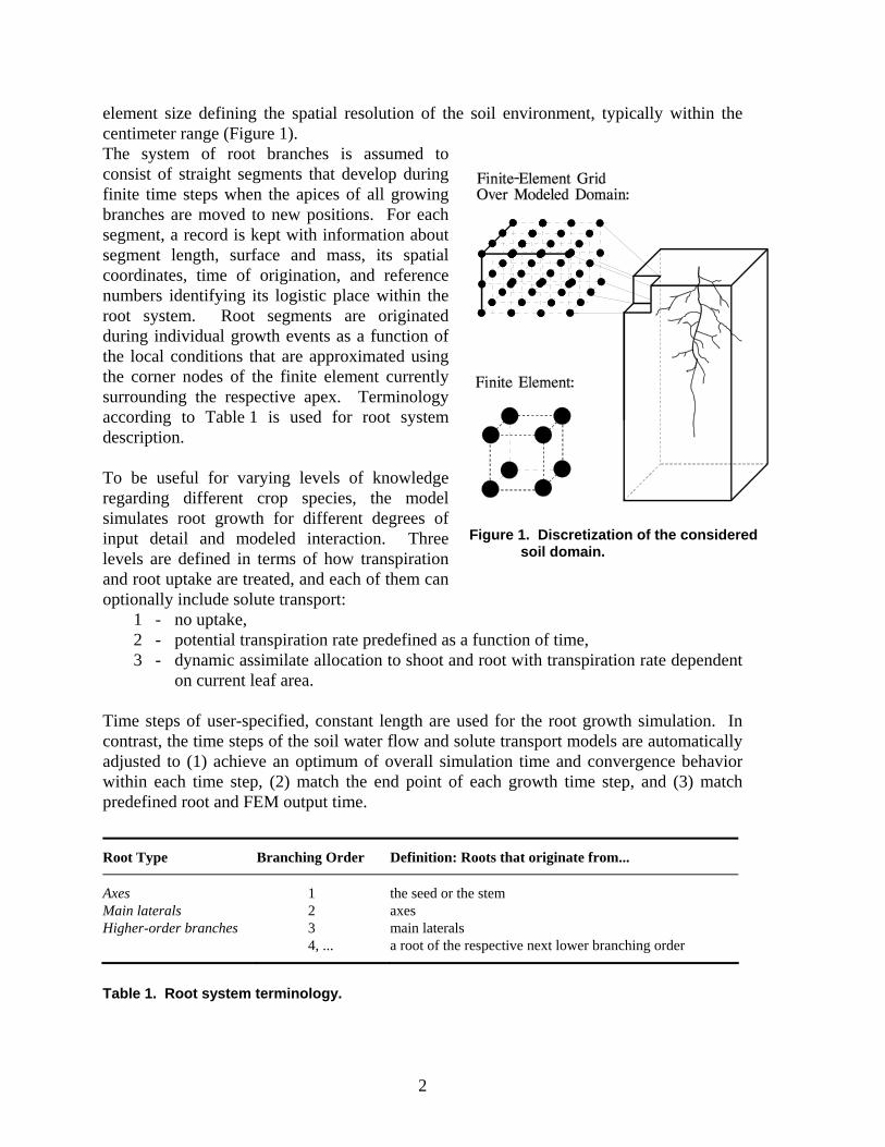
element size defining the spatial resolution of the soil environment, typically within the centimeter range (Figure 1). The system of root branches is assumed to consist of straight segments that develop during finite time steps when the apices of all growing branches are moved to new positions. For each segment, a record is kept with information about segment length, surface and mass, its spatial coordinates, time of origination, and reference numbers identifying its logistic place within the root system. Root segments are originated during individual growth events as a function of the local conditions that are approximated using the corner nodes of the finite element currently surrounding the respective apex. Terminology according to Table 1 is used for root system description. To be useful for varying levels of knowledge regarding different crop species, the model simulates root growth for different degrees of input detail and modeled interaction. Three levels are defined in terms of how transpiration and root uptake are treated, and each of them can optionally include solute transport:

1 - no uptake, 2 - potential transpiration rate predefined as a function of time, 3 - dynamic assimilate allocation to shoot and root with transpiration rate dependent

on current leaf area. Time steps of user-specified, constant length are used for the root growth simulation. In contrast, the time steps of the soil water flow and solute transport models are automatically adjusted to (1) achieve an optimum of overall simulation time and convergence behavior within each time step, (2) match the end point of each growth time step, and (3) match predefined root and FEM output time. Root Type Branching Order Definition: Roots that originate from... Axes Main laterals Higher-order branches

1 2 3 4, ...

the seed or the stem axes main laterals a root of the respective next lower branching order

Table 1. Root system terminology.

Figure 1. Discretization of the considered

soil domain.

3

Plant-defining input includes both single-valued parameters and genotype-specific functions. For maximum flexibility, plant input functions are specified as a series of data points; function values between specified points are obtained from linear interpolation. The number of specified points is arbitrary; well-known relationships can thus be described more closely by simply providing more data points. Output can be obtained at any time during the simulation and includes files describing the root system at that particular point in time, as well as a list of the nodal soil water content, pressure head and water uptake rate values from the FEM flow model and nodal concentrations and solute uptake rate values from the FEM solute transport model and absolute and relative errors in water and solute mass balances. Both root system and FEM output files can later be directly used as input files, permitting easy continuation of any previously terminated simulation. For example, a root system obtained from one simulation can serve as input for subsequent simulations when it is desirable to study the effects of different environmental scenarios with an initial root system that is already developed. Soil Water Flow The flow model solves the three-dimensional form of the Richards' equation for soil water pressure head h [L] (negative in unsaturated porous media):

∂θ∂t =

∂∂xi

⎣⎢⎡

⎦⎥⎤K

⎝⎜⎛

⎠⎟⎞K

Aij

∂h∂xj

+ K Aiz – S ; (1)

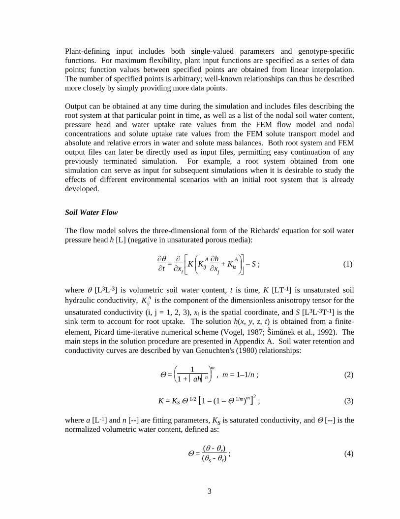
where θ [L3L-3] is volumetric soil water content, t is time, K [LT-1] is unsaturated soil hydraulic conductivity, Kij

A is the component of the dimensionless anisotropy tensor for the unsaturated conductivity (i, j = 1, 2, 3), xi is the spatial coordinate, and S [L3L-3T-1] is the sink term to account for root uptake. The solution h(x, y, z, t) is obtained from a finite-element, Picard time-iterative numerical scheme (Vogel, 1987; S

vimu°nek et al., 1992). The

main steps in the solution procedure are presented in Appendix A. Soil water retention and conductivity curves are described by van Genuchten's (1980) relationships:

Θ = ⎝⎜⎛

⎠⎟⎞1

1 + ⎪ah⎪n

m , m = 1–1/n ; (2)

K = KS Θ 1/2 [ ]1 – (1 – Θ 1/m)m 2

; (3) where a [L-1] and n [--] are fitting parameters, Ks is saturated conductivity, and Θ [--] is the normalized volumetric water content, defined as:

Θ = (θ - θr)(θs - θr)

; (4)

4

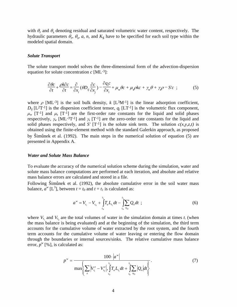
with θr and θs denoting residual and saturated volumetric water content, respectively. The hydraulic parameters θr, θs, a, n, and Ks have to be specified for each soil type within the modeled spatial domain. Solute Transport The solute transport model solves the three-dimensional form of the advection-dispersion equation for solute concentration c [ML-3]:

∂θc∂t +

ρk∂c∂t =

∂∂xi

(θDij ∂c∂xj

) – ∂qic∂xi

+ µwθc + µsρkc + γwθ + γsρ – S'c ; (5)

where ρ [ML-3] is the soil bulk density, k [L3M-1] is the linear adsorption coefficient, Dij [L2T-1] is the dispersion coefficient tensor, qj [LT-1] is the volumetric flux component, µw [T-1] and µs [T-1] are the first-order rate constants for the liquid and solid phases respectively, γw [ML-3T-1] and γs [T-1] are the zero-order rate constants for the liquid and solid phases respectively, and S' [T-1] is the solute sink term. The solution c(x,y,z,t) is obtained using the finite-element method with the standard Galerkin approach, as proposed by S

vimu°nek et al. (1992). The main steps in the numerical solution of equation (5) are

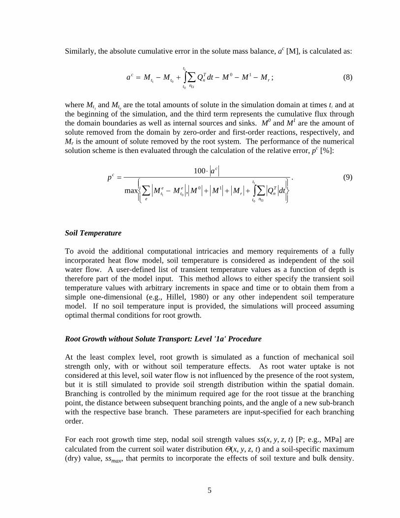
presented in Appendix A. Water and Solute Mass Balance To evaluate the accuracy of the numerical solution scheme during the simulation, water and solute mass balance computations are performed at each iteration, and absolute and relative mass balance errors are calculated and stored in a file. Following S

vimu°nek et al. (1992), the absolute cumulative error in the soil water mass

balance, aw [L3], between t = t0 and t = t1 is calculated as:

a V V T L dt Q dtwt t a t n

nt

t

t

t

= − + − ∑∫∫1 0 1

0

1

0

1

Ω

; (6)

where Vt1

and Vt0 are the total volumes of water in the simulation domain at times t1 (when

the mass balance is being evaluated) and at the beginning of the simulation, the third term accounts for the cumulative volume of water extracted by the root system, and the fourth term accounts for the cumulative volume of water leaving or entering the flow domain through the boundaries or internal sources/sinks. The relative cumulative mass balance error, pw [%], is calculated as:

pa

V V T L dt Q dt

ww

te

te

ea t

t

t

nnt

t=

⋅

− +⎧⎨⎪

⎩⎪

⎫⎬⎪

⎭⎪∑ ∫ ∑∫

100

1 0 1

0

1

0

1

max ,Ω

. (7)

5

Similarly, the absolute cumulative error in the solute mass balance, ac [M], is calculated as:

a M M Q dt M M Mct t n

T

nt

t

r= − + − − −∑∫1 0

0

10 1

Ω

; (8)

where Mt1

and Mt0 are the total amounts of solute in the simulation domain at times t1 and at

the beginning of the simulation, and the third term represents the cumulative flux through the domain boundaries as well as internal sources and sinks. M0 and M1 are the amount of solute removed from the domain by zero-order and first-order reactions, respectively, and Mr is the amount of solute removed by the root system. The performance of the numerical solution scheme is then evaluated through the calculation of the relative error, pc [%]:

pa

M M M M M Q dt

cc

te

te

er n

T

nt

t=

⋅

− + + +⎧⎨⎪

⎩⎪

⎫⎬⎪

⎭⎪∑ ∑∫

100

1 0

0

10 1max ,

Ω

. (9)

Soil Temperature To avoid the additional computational intricacies and memory requirements of a fully incorporated heat flow model, soil temperature is considered as independent of the soil water flow. A user-defined list of transient temperature values as a function of depth is therefore part of the model input. This method allows to either specify the transient soil temperature values with arbitrary increments in space and time or to obtain them from a simple one-dimensional (e.g., Hillel, 1980) or any other independent soil temperature model. If no soil temperature input is provided, the simulations will proceed assuming optimal thermal conditions for root growth. Root Growth without Solute Transport: Level '1a' Procedure At the least complex level, root growth is simulated as a function of mechanical soil strength only, with or without soil temperature effects. As root water uptake is not considered at this level, soil water flow is not influenced by the presence of the root system, but it is still simulated to provide soil strength distribution within the spatial domain. Branching is controlled by the minimum required age for the root tissue at the branching point, the distance between subsequent branching points, and the angle of a new sub-branch with the respective base branch. These parameters are input-specified for each branching order. For each root growth time step, nodal soil strength values ss(x, y, z, t) [P; e.g., MPa] are calculated from the current soil water distribution Θ(x, y, z, t) and a soil-specific maximum (dry) value, ssmax, that permits to incorporate the effects of soil texture and bulk density.

6

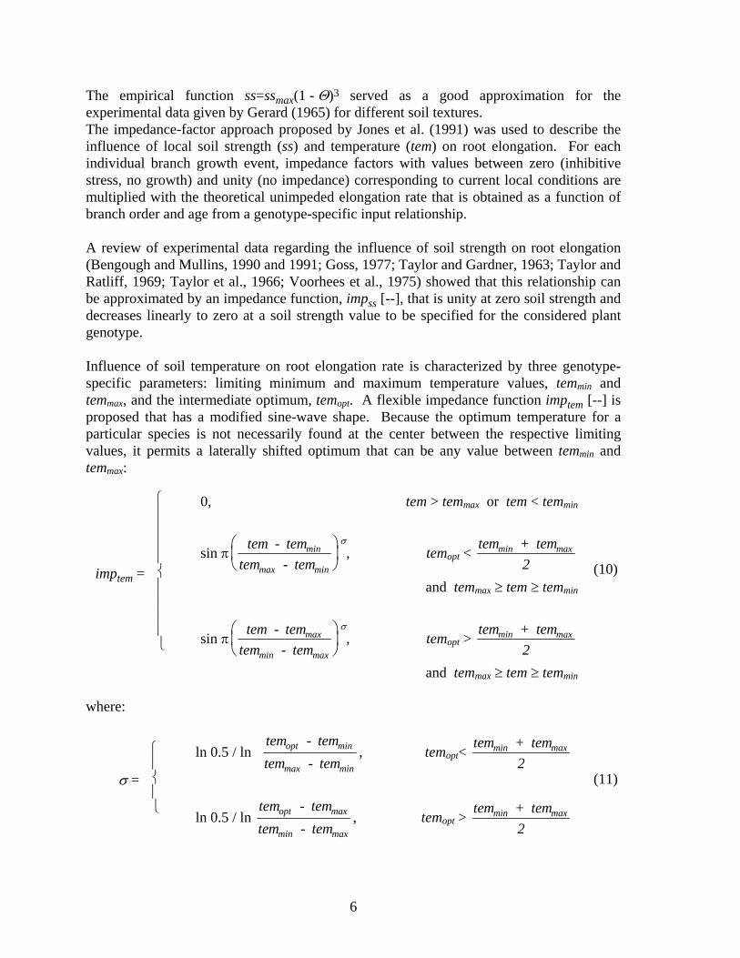
The empirical function ss=ssmax(1 - Θ)3 served as a good approximation for the experimental data given by Gerard (1965) for different soil textures. The impedance-factor approach proposed by Jones et al. (1991) was used to describe the influence of local soil strength (ss) and temperature (tem) on root elongation. For each individual branch growth event, impedance factors with values between zero (inhibitive stress, no growth) and unity (no impedance) corresponding to current local conditions are multiplied with the theoretical unimpeded elongation rate that is obtained as a function of branch order and age from a genotype-specific input relationship. A review of experimental data regarding the influence of soil strength on root elongation (Bengough and Mullins, 1990 and 1991; Goss, 1977; Taylor and Gardner, 1963; Taylor and Ratliff, 1969; Taylor et al., 1966; Voorhees et al., 1975) showed that this relationship can be approximated by an impedance function, impss [--], that is unity at zero soil strength and decreases linearly to zero at a soil strength value to be specified for the considered plant genotype. Influence of soil temperature on root elongation rate is characterized by three genotype-specific parameters: limiting minimum and maximum temperature values, temmin and temmax, and the intermediate optimum, temopt. A flexible impedance function imptem [--] is proposed that has a modified sine-wave shape. Because the optimum temperature for a particular species is not necessarily found at the center between the respective limiting values, it permits a laterally shifted optimum that can be any value between temmin and temmax:

imptem =

⎧ ⎪ ⎪ ⎪ ⎪ ⎨ ⎪ ⎪ ⎪ ⎪ ⎩

0, tem > temmax or tem < temmin

sin π tem - temtem - tem

min

max min

⎛

⎝⎜

⎞

⎠⎟

σ, temopt < tem + tem

2min max

and temmax ≥ tem ≥ temmin

sin π tem - temtem - tem

max

min max

⎛

⎝⎜

⎞

⎠⎟

σ, temopt > tem + tem

2min max

and temmax ≥ tem ≥ temmin

(10)

where:

σ =

⎧ ⎪ ⎨ ⎪ ⎩

ln 0.5 / ln tem - temtem - tem

opt min

max min, temopt< tem + tem

2min max

ln 0.5 / ln tem - temtem - tem

opt max

min max, temopt > tem + tem

2min max

(11)

7

Thus, imptem is zero at the limits, and unity at temopt. Elongation rate and length of the growth time step define the length of each new segment. Root mass per unit length is taken as a user-defined function of the current local soil strength for each branching order; this permits to account for root thickening at high soil strength. Following Pages et al. (1989), the vector defining the growth direction of a particular apex is obtained by adding individual direction-affecting components. For the present model, these include: − the direction of the preceding root segment, changed by a limited random deviation as

an computationally effective means for approximating the space-exploring nature of root system growth,

− geotropism along an angle with the horizontal plane that is user-specified for each axis group and the main laterals,

− the (negative) current local soil strength gradient. The magnitudes of the second and third components relative to the first component are defined by weighting factors for each branching order. Setting the respective weighting factor to zero permits the elimination of either of the latter components for selected branching orders. Experimental evidence (Mosher and Miller, 1972; Horwitz and Zur, 1991; Fortin and Poff, 1990; Kaspar and Bland, 1992; Kutschera-Mitter, 1971, 1972, 1973, and 1976) suggests that soil temperature has an important effect on plant root geotropism. The model therefore permits to define a vertical geotropic growth angle as a function of soil temperature for axes and second-order branches. For efficiency, axes can be assigned to groups of similar geotropic response. Root Growth with Solute Transport: Level '1b' Procedure Excessive or deficient nutrient concentration effects on root growth rate are considered at this level. Root growth rates are unaffected by nutrient availability as long as the latter is maintained within an optimal range (i.e. concentration values c are maintained between optimal minimum and maximum values coptmin and coptmax). Growth rate rapidly decreases outside the optimal range and completely ceases if concentration values are above or below the maximum and the minimum values tolerated, cmax and cmin, respectively (Bloom et al., 1993). As optimal range and minimum and maximum concentration are both genotype and nutrient specific, the effects of nutrient concentration are simulated using a piecewise linear impedance function, impc [--]. The function varies linearly between zero (c ≤ cmin or cmax ≤ c, no growth) and unity (optimal concentration range, no impedance). Thus, at each growth event, the actual root elongation rate is obtained by multiplying the theoretical unimpeded elongation rate with the three current values of the impedance factors impc, imps, and impt, the latter two described in the previous paragraph. As root solute uptake is not considered at this level, solute transport is not influenced by the presence of the root system, but it is simulated to determine concentration distribution

8

within the spatial domain for the computation of nodal values of the impedance function impc. Alternatively, the option is offered to consider nutrient concentration effects without simulating solute transport by specifying in the FEM input file an initial concentration distribution, which is kept constant throughout the simulation: effects of excessive or deficient nutrient concentration on root growth rate can thus be accounted for at any of the six simulation levels. Water Uptake: Level '2a' Procedure Level '2a' simulates root growth similar to level '1a', but also includes root water uptake and water loss to the atmosphere. To eliminate evaporation as a variable, all model simulations are performed for a plastic-covered soil surface. The single-plant scale of the model and the conceptual insulation of the modeled soil domain (except for optional irrigation) make it useful to express Tpot as a volumetric flow rate [L3T-1] rather than depth per unit of time typical for field-scale considerations. By assuming a growth chamber environment with a controlled regime of temperature, wind, humidity, radiation, and atmospheric carbon dioxide concentration, a potential transpiration rate Tpot can be defined as a function of time (i.e., age) for the considered plant and determined experimentally for nonlimiting soil water conditions. It should be recognized that a Tpot time-function defined in this manner will already include all stomata closure effects other than those due to low soil water potential. Thus Tpot effectively becomes a prespecified time-varying boundary condition for level '2' simulations. The spatial resolution of the soil domain given by the finite-element grid, root water uptake in the vicinity of each node are lumped into the sink terms S(x, y, z, t) of the respective node. The set of nodal S-values is updated at each time step during the simulation using the procedure explained hereafter. A localized form of the extraction function is used to account for the local influence of soil water potential on the root water uptake rate. A value α (x, y, z, t) [--] representing this function is calculated at each node using the expression proposed by van Genuchten (1987), which considers the effects of water and osmotic potential on the uptake rate to be multiplicative:

( )[ ] ( )[ ]α

π π(x, y, z, t)

1

1 h / h * 1 /50p1

50p2=

+ +; (12)

where h50 and π50 are, respectively, the pressure head and the osmotic head at which the uptake rate is reduced by 50% and p1 and p2 are two fitting parameters, usually found to be approximately 3 (van Genuchten and Gupta, 1993). The option is provided to account for pressure head effects only, using the expression proposed by van Genuchten:

9

( )[ ]α(x,y,z, t)

1

1 h / h50p1=

+; (13)

or the expression by Feddes et al. (1978), shown in Figure 2. For various alternative extraction functions, see the review by Molz (1981).

0.0

0.2

0.4

0.6

0.8

1.0

1.2

Pressure head h

α(h)

h4 h3 h2 h1

Figure 2. Water stress response function (Feddes et al., 1978)

Current distribution of potential root water uptake sites within the soil domain is lumped into nodal values of a function β(x, y, z, t) [--]. Uptake site spatial distribution may be a function of plant and soil conditions. As the model explicitly records length, age and position of each root segment, it is well-suited for implementation and testing of different methods to calculate β(x, y, z, t). This function is constructed by identifying the finite element that surrounds the root segment and subsequently contributing to each of its eight corner nodes a value that is equal to the inverse distance between the center of the segment and the respective corner and proportional to the segment length. Root uptake patterns may vary along the root axis, mainly as a function of age (Henriksen et al., 1992; Lazof et al., 1992). Thus, a set of piecewise linear weighting functions allows to account for each branch segment according to its age and branching order. Each segment in the root system can be therefore fully accounted for, or be partially or totally excluded from uptake by setting its weight to any value between unity and zero. If a segment does not entirely lie within the finite element in which it originates, all the finite elements containing a portion of the segment are identified, and the procedure outlined above is applied to each of the sub-segments. When completed, the β-value of a particular node will increase as the number of active root segments and their respective lengths within its neighboring elements increase; the β-value of the node also increases as its respective distances to the centerpoints of those segments decrease. Regardless of how the β(x, y, z, t) function is calculated, it needs to be normalized so that its integral over the spatial domain D becomes equal to unity. Thus, a function β '(x, y, z, t) [L-3] is obtained from:

β' = β(x,y,z)

⌡⌠D

β(x,y,z)dD ; (14)

10

which permits to take α(x, y, z, t)β '(x, y, z, t) as a representation of the current uptake intensity distribution. The sink term S(x, y, z, t) to be used in (1) is obtained from: S(x, y, z, t) = α(x, y, z, t)β '(x, y, z, t)Tpot . (15) The actual transpiration rate, defined as Tact =⌡⌠

D

S(x, y, z, t)dD , will equal Tpot if α(x, y, z, t)

is equal to unity throughout D. Solute Uptake: Level '2b' Procedure At this level solute transport is being included in the simulation. Root solute uptake throughout the domain is lumped into nodal values of the sink term S'(x,y,z,t) (see equation 5), expressed as: S' S A= + −δ δ(1 ) ; (16) where δ [--] is a partition coefficient. The first term of the right-hand side refers to passive uptake (S is calculated according to eq. (15)), while the second one refers to active uptake. Experimental results (Kochian and Lucas, 1982; Siddiqi et al., 1990) have shown that the kinetics of active uptake is best described by the sum of a Michaelis-Menten component (Barber, 1984) and a linear component (Kochian and Lucas, 1982):

AV

K cf R

md=

++( )max ; (17)

where Vmax [ML-2T-1] is the maximum uptake rate, Km [ML-3] the Michaelis-Menten constant, Rd [L2L-3] the rooting density, and f is the first-order rate coefficient [LT-1]. The rooting density function Rd is computed at each time step as: Rd (x,y,z) = Ts σ'( x,y,z) ; (18) where Ts [L2] is the total root surface at the current time and σ' [L-3] is a function describing the current distribution of potential solute uptake sites within the domain. The function σ' is similar to the β ' function in the previous paragraph, except that nodal values are now proportional to the segments' surface area rather than their length. Shoot and Root Growth without Solute Transport: Level '3a' Procedure Provided sufficient information is available for a particular plant species, a level '3' simulation can be attempted that is more comprehensive and also includes growth of the shoot. In contrast to levels '1' and '2', root growth will be limited by the amount of assimilate allocated to the root at each growth time step. At a given growth time step, first the root growth procedure as described for level '1' is followed to calculate the potential

11

need for new root assimilates according to the current soil strength and soil temperature conditions. If the amount of assimilate allocated to the root is smaller than the potential need, all new segments will be scaled back accordingly. In case of surplus allocation, the extra assimilate is assumed to be exuded by the root. Smucker (1984) lists reported root exudation data approximately ranging from 20% to 50% of total root-allocated assimilate. The model software continually logs the allocation/need ratio to an output file because it provides a check on the consistency of the input parameters for a level '3a' simulation. For consistent input, the relative surplus should not substantially exceed the quoted range.

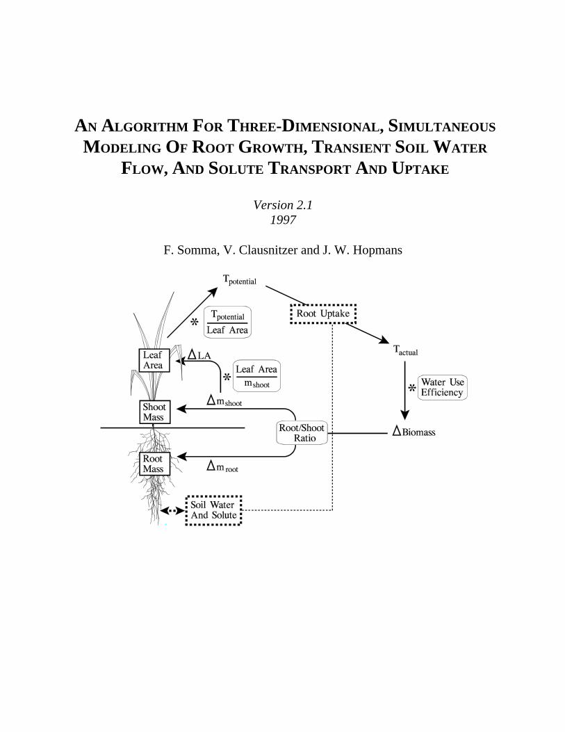
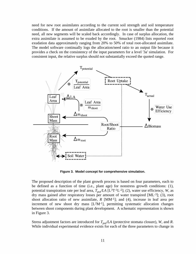
Figure 3. Model concept for comprehensive simulation. The proposed description of the plant growth process is based on four parameters, each to be defined as a function of time (i.e., plant age) for nonstress growth conditions: (1), potential transpiration rate per leaf area, Tpot/LA [L3T-1L-2]; (2), water use efficiency, W, as dry mass gained after respiratory losses per amount of water transpired [ML-3]; (3), root shoot allocation ratio of new assimilate, R [MM-1]; and (4), increase in leaf area per increment of new shoot dry mass [L2M-1], permitting systematic allocation changes between shoot components during plant development. A schematic representation is shown in Figure 3. Stress adjustment factors are introduced for Tpot/LA (protective stomata closure), W, and R. While individual experimental evidence exists for each of the three parameters to change in

12

response to external stresses (Lafolie et al., 1991, and references given therein; Masle, 1992; Masle and Passioura, 1987; Masle et al., 1990; Tucker and von Seelhorst, 1898), the mechanisms and message pathways are not yet well understood. To permit flexible testing of the interplay of theoretical response patterns, the stress adjustment factors can be arbitrarily defined as a piecewise-linear function of relative plant stress. At the current simulation level the relative stress is computed solely as a function of the average soil strength experienced by the root system and thus accounts for stress effects due to soil water potential and mechanical root growth resistance. This function is also of user-specified, piecewise-linear shape. During the simulation, the current value of each stress-influenced parameter is obtained by multiplying the nonstress parameter value at the current time with the respective adjustment factor representative of the current stress conditions. Root water uptake is modeled similar to level '2' except for Tpot, which will depend on the current leaf area rather than being a predescribed time-function. Under the level '3a' concept, the potential for new growth increases as the existing leaf area increases. Thus simulated growth curves will approximately follow the exponential shape that is typical for natural growth processes. Shoot and Root Growth with Solute Transport: Level '3b' Procedure At the most complex level, solute transport is included in the simulation. Root and shoot growth are simulated as described in the previous paragraph, but a new set of stress factors is introduced to simulate the effects of deficient or excessive solute concentration on plant growth. Specifically, stress adjustment factors have been added for Tpot/LA, W and R. While the effect of solute concentration on each of these parameters has been described (Schmidhalter and Oertli, 1991; Stark, 1992; Ericsson, 1995), the combined effects and, moreover, the interaction with other stress causes (i.e. soil strength, water deficiency, temperature, etc.) is still subject of intense studies. At this stage the stress factors are described by piecewise-linear functions of relative stress due to solute concentration. The function describing relative stress due to solute concentration is, in turn, also described by a piecewise-linear function. When both soil strength and solute concentration stress affect one of the three growth parameters, only the most limiting between the two stress adjustment factors is taken into account (Jones et al., 1991). As in the previous level, during the simulation, the current value of each stress-influenced parameter is obtained by multiplying the nonstress parameter value at the current time with the respective adjustments factors (one function of soil strength an another function of solute concentration) representative of the current stress conditions. Thus, the effects of soil strength and solute concentration stress on each of the three parameters have been considered at this stage as multiplicative. Passive root solute uptake is modeled similar to level '2' except for Tpot, which will depend on the current leaf area rather than being a predescribed time-function.

13

III. PREPROCESSING AND MODEL INPUT The following input files are required to run the simulation program:

− grid.in − file containing a list of all nodal coordinates, soil type and initial soil water

pressure head values (name specified by user) − bc.in − soil.in − chem.in (optional) − control.in − plant.in (optional) − tpot.in (optional) − root.in − temp.in (optional) − file defining the initial root system (name specified by user)

This section explains the purpose and contents of each of these files. Commenting lines are provided in all input files to enhance readability and to support editing by the user. Creating the FEM Grid The preprocessor grid.for (Appendix D) discretizes the considered soil domain into a rectangular grid with user-defined node spacing. In addition to its spatial coordinates (x, y, z), each node is assigned an initial soil water pressure head and concentration value (initial condition, I.C.) and a reference number for the soil type assumed at this point in space. In that the nodal I.C. and soil type values are application-specific, grid.for will usually have to be edited to make the necessary changes in the lines indicated by the comment line in the source code. The application-specific statements are located within the loop that calculates the nodal coordinates, immediately before the WRITE statement is executed that adds the values for the current node as a new line to the input file. At this point, soil type and I.C. values can easily be assigned to the current node using IF statements conditioned by the nodal (x, y, z) coordinates. Once the appropriate changes have been made, grid.for can be compiled, linked and executed. It will first prompt the user to specify names for the two files it will create. The first file contains the global grid parameters and a list of all finite elements and their respective corner nodes. The main program expects this file to be present as 'grid.in'. The second file, consisting of a list of all nodal coordinates, soil type and I.C. values, can be named arbitrarily because the main program will prompt for its name. The preprocessor will then require user input for the (constant) node spacing for each spatial direction (dx, dy, dz) within the rectangular grid and the number of nodes in each direction. The last user input specifies the (x, y, z) coordinates of the first node which is defined to be the node at the upper-left corner of the domain (minimum x and y, maximum z, with z defined positive upward).

14

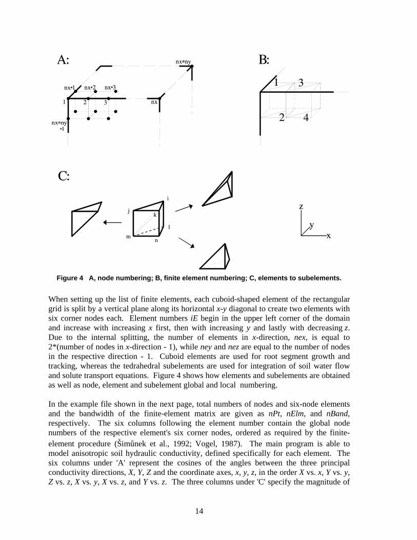
Figure 4 A, node numbering; B, finite element numbering; C, elements to subelements.

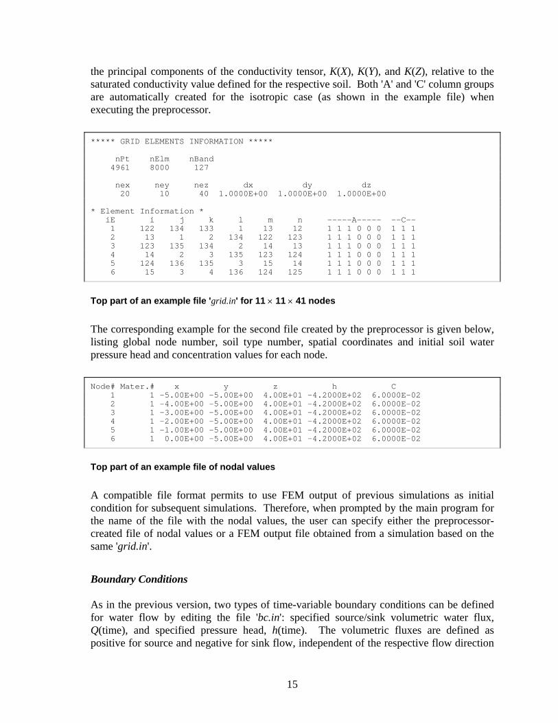
When setting up the list of finite elements, each cuboid-shaped element of the rectangular grid is split by a vertical plane along its horizontal x-y diagonal to create two elements with six corner nodes each. Element numbers iE begin in the upper left corner of the domain and increase with increasing x first, then with increasing y and lastly with decreasing z. Due to the internal splitting, the number of elements in x-direction, nex, is equal to 2*(number of nodes in x-direction - 1), while ney and nez are equal to the number of nodes in the respective direction - 1. Cuboid elements are used for root segment growth and tracking, whereas the tedrahedral subelements are used for integration of soil water flow and solute transport equations. Figure 4 shows how elements and subelements are obtained as well as node, element and subelement global and local numbering. In the example file shown in the next page, total numbers of nodes and six-node elements and the bandwidth of the finite-element matrix are given as nPt, nElm, and nBand, respectively. The six columns following the element number contain the global node numbers of the respective element's six corner nodes, ordered as required by the finite-element procedure (S

vimu°nek et al., 1992; Vogel, 1987). The main program is able to

model anisotropic soil hydraulic conductivity, defined specifically for each element. The six columns under 'A' represent the cosines of the angles between the three principal conductivity directions, X, Y, Z and the coordinate axes, x, y, z, in the order X vs. x, Y vs. y, Z vs. z, X vs. y, X vs. z, and Y vs. z. The three columns under 'C' specify the magnitude of

15

the principal components of the conductivity tensor, K(X), K(Y), and K(Z), relative to the saturated conductivity value defined for the respective soil. Both 'A' and 'C' column groups are automatically created for the isotropic case (as shown in the example file) when executing the preprocessor. ***** GRID ELEMENTS INFORMATION ***** nPt nElm nBand 4961 8000 127 nex ney nez dx dy dz 20 10 40 1.0000E+00 1.0000E+00 1.0000E+00 * Element Information * iE i j k l m n -----A----- --C-- 1 122 134 133 1 13 12 1 1 1 0 0 0 1 1 1 2 13 1 2 134 122 123 1 1 1 0 0 0 1 1 1 3 123 135 134 2 14 13 1 1 1 0 0 0 1 1 1 4 14 2 3 135 123 124 1 1 1 0 0 0 1 1 1 5 124 136 135 3 15 14 1 1 1 0 0 0 1 1 1 6 15 3 4 136 124 125 1 1 1 0 0 0 1 1 1

Top part of an example file 'grid.in' for 11 × 11 × 41 nodes The corresponding example for the second file created by the preprocessor is given below, listing global node number, soil type number, spatial coordinates and initial soil water pressure head and concentration values for each node. Node# Mater.# x y z h C 1 1 -5.00E+00 -5.00E+00 4.00E+01 -4.2000E+02 6.0000E-02 2 1 -4.00E+00 -5.00E+00 4.00E+01 -4.2000E+02 6.0000E-02 3 1 -3.00E+00 -5.00E+00 4.00E+01 -4.2000E+02 6.0000E-02 4 1 -2.00E+00 -5.00E+00 4.00E+01 -4.2000E+02 6.0000E-02 5 1 -1.00E+00 -5.00E+00 4.00E+01 -4.2000E+02 6.0000E-02 6 1 0.00E+00 -5.00E+00 4.00E+01 -4.2000E+02 6.0000E-02

Top part of an example file of nodal values A compatible file format permits to use FEM output of previous simulations as initial condition for subsequent simulations. Therefore, when prompted by the main program for the name of the file with the nodal values, the user can specify either the preprocessor-created file of nodal values or a FEM output file obtained from a simulation based on the same 'grid.in'. Boundary Conditions As in the previous version, two types of time-variable boundary conditions can be defined for water flow by editing the file 'bc.in': specified source/sink volumetric water flux, Q(time), and specified pressure head, h(time). The volumetric fluxes are defined as positive for source and negative for sink flow, independent of the respective flow direction

16

(i.e., a source flow rate will always be positive, whether applied at the surface or at the bottom of the soil domain). Both types of boundary conditions are described by a list of paired values defining a piecewise linear function. During program execution, the then-current simulation time is used to interpolate the given values. When the simulation time exceeds the time value of the last (time, B.C.) value pair, the B.C. value of the last pair is applied. In addition, the current version of the program allows to specify a unit vertical gradient B.C. to simulate free drainage at the bottom of the domain or at a portion of it. ***** BC INFORMATION ***** * Water flux B.C.'s * Number of Q-Boundary Nodes: 5 List of Q-Boundary Nodes: 50 60 61 62 72 Number of (Time;Q)-points (prescribed water flux): 2 List of (Time;Q)-points [T]; [L3/T]: .0 .0 50. .30 * Head B.C.'s * Number of h-Boundary Nodes: 0 List of h-Boundary Nodes: --- Number of (Time;h)-points (prescribed pressure head): 0 List of (Time;h)-points [T]; [L]: --- * Free drainage nodes: Number of free drainage nodes: 0 List of free drainage nodes: --- * Nodal solute transport B.C.'s assignment code: -1 -1 -1 -1 -1 Number of (Time;c)-points (first time dependent B.C.): 1 List of (Time;c)-points [T]; [microMole/L3]: 0.0 1. Number of (Time;c)-points (second time dependent B.C.): 0 List of (Time;c)-points [T]; [microMole/L3]: --- * Pulse duration [T] 600.

Example file 'bc.in' For each water flow B.C.(time) function, a list of global node numbers defines the nodes at which the respective boundary condition applies. A "zero external source/sink" condition applies at all nodes not specified in 'bc.in'.

17

Two types of time-variable boundary conditions can be specified for solute transport at each of the nodes for which a water flow B.C. (pressure head or flux) has been assigned. The B.C. type depends on the sign given to B.C. code: a positive sign refers to a concentration B. C., c(time) (Dirichlet type), whereas a negative sign implies a solute flux B.C., Qc(time) (Neumann type if the water flux at that node is zero or directed out of the region, Cauchy type if the water flux is directed into the region). The value of the assignment code refers to which of the two piecewise linear B.C. is being assigned to each node. Each of the two B.C. is always expressed in units of concentration; if used to express a solute flux B.C., it is later multiplied with the then-current water flux during the execution of the subroutine c_bound, which incorporates the B.C.s into the FEM system of equations. The number of piecewise linear B.C. functions can be increased to more than two, provided that the corresponding arrays are expanded in the source code. In the last line of the file the time duration of the concentration pulse is specified. Soil Parameters The parameters defining van Genuchten's (1980) soil hydraulic functions, θr, θs, a, n, and Ks, as well as the maximum soil strength are listed in file 'soil.in'. If more than one soil type is present within the modeled soil domain, the parameter values for soil type number two are listed as the second line of parameters, those for number three as the third line, etc. For faster program execution, an internal interpolation table for each soil-type's soil hydraulic conductivity and soil water capacity functions is created. The values hTab1 and hTab2 denote the two limiting soil water pressure head values for this interpolation table. Independent of how they are specified in 'soil.in', they are always converted to negative values. During the FEM iterations, only for pressure head values outside the tabulated range will the hydraulic functions be evaluated directly. ***** SOIL PARAMETERS ***** hTab1[L] hTab2[L] .01 1000. thr[L3/L3] ths[L3/L3] a[1/L] n Ks[L/T] ssMax[P] .0 .55 .003 3.0 .75 12.0

Example file 'soil.in' with parameters for one soil type Solute Transport Parameters The file 'chem.in' lists the parameters necessary for solving the transport equation. In the first line, the value of the temporal weighting coefficient to be used for approximation of the time derivatives in the equation is specified. The second line contains the parameter PeCr, used as stability criterion for the solute transport scheme. The third line contains the bulk density of the soil ρ, the molecular diffusion coefficient Dd, the transversal and

18

longitudinal dispersivities DL and DT, the linear adsorption coefficient k and the first and zero-order rate constants µw, µs, γw, γ (see Eq. (5)). Similar to 'soil.in', as many sets of parameters will be specified in the file as many soil types are considered in the simulation domain. If 'chem.in' is not provided a message is sent to the console informing the user that solute transport is not considered. ******** Solute transport parameters ******** Temporal weighing coefficient (1.=implicit, 0.=explicit, .5=Crank-Nicholson) 0.5 PeCr 1.5 Bulk d. Diff. Disper. Adsorp. SinkL1 SinkS1 SinkL0 SinkS0 [M/L3] [L2/T] [L] [L3/M] [1/T] [1/T] [M/L3T] [1/T] 1.53 0.0684 .5 .1 .0 .0 .0 .0 .0

Example file 'chem.in'

Execution Control The input file 'control.in' comprises application-specific user information and parameters controlling both the FEM iteration process and the program output events. The third line of the file may contain up to eighty characters between the single quotation marks. This text string will become the headline for each FEM output file. The length, time, mass and concentration units used in the simulation can be specified in line six by up to five characters each. For additional information, they are also embedded in the top part of each FEM output file. The parameters itMax and epslon denote the maximum permitted number of iterations per FEM time step and the convergence criterion for FEM time step iterations (maximum permitted change in nodal pressure head). The initial time step length for the FEM procedures of the soil water flow model is defined as dt. During the simulation, this time step length is constantly adjusted to optimize the convergence of the FEM iterations. Time step length is increased by the factor FacInc if convergence was obtained quickly during the previous time step (i.e., less than four iterations) and decreased by FacDec if convergence was slow (i.e., more than six iterations). The smallest and greatest permitted time step lengths are given as dtMin and dtMax, respectively. The constant time interval between subsequent root growth events is defined as dtRoot. The last part of 'control.in' contains the lists of times at which FEM and/or root system output files are to be created.

19

***** APPLICATION CONTROL PARAMETERS ***** '10 x 10 x 40 Column' Units [L] [T] [M] Concentration: 'cm' 'hours' 'g' 'microMole/cm3' itMax epslon 20 .01 dt dtMin dtMax FacInc FacDec dtRoot 4. .0001 10. 1.1 0.9 12. Number of FEM-Outputs: 7 FEM-Output at time: 50. 100. 200. 300. 400. 500. 600. Number of Root-Outputs: 7 Root-Output at time: 50. 100. 200. 300. 400. 500. 600.

Example file 'control.in' Plant Growth Parameters The program automatically runs a level '3' simulation if it finds the file 'plant.in' to be present. This input file contains time and stress functions that may be specific for each particular plant species. For maximum flexibility, these functions are specified as a series of data points; during the simulation, function values between specified points are obtained from linear interpolation. The number of specified points is arbitrary; well-known relationships can thus be described more closely by simply providing more function points. The first three blocks of 'plant.in' cover three time-depending basic nonstress growth parameters, each described by a list of paired values defining a piecewise linear function of time. During program execution, the then-current simulation time is used to interpolate the given parameter values. When the simulation time exceeds the time value of the last value pair for one of the three functions, the functional value of the respective last pair is applied. The next four blocks contain the stress influence factors due to soil strength stress for each of these three basic growth parameters and the respective relative-stress function. Each of the three factors is described by a list of paired values defining a piecewise linear function of relative stress. Four additional blocks describe the stress influence factors due to solute concentration for each of these three basic growth parameters and the respective relative-stress function. Again, each of the three factors is described by a list of paired values defining a piecewise linear function of relative stress. The last block contains the list of paired values defining the increase in leaf area per increment of new shoot mass as a piecewise linear function of time.

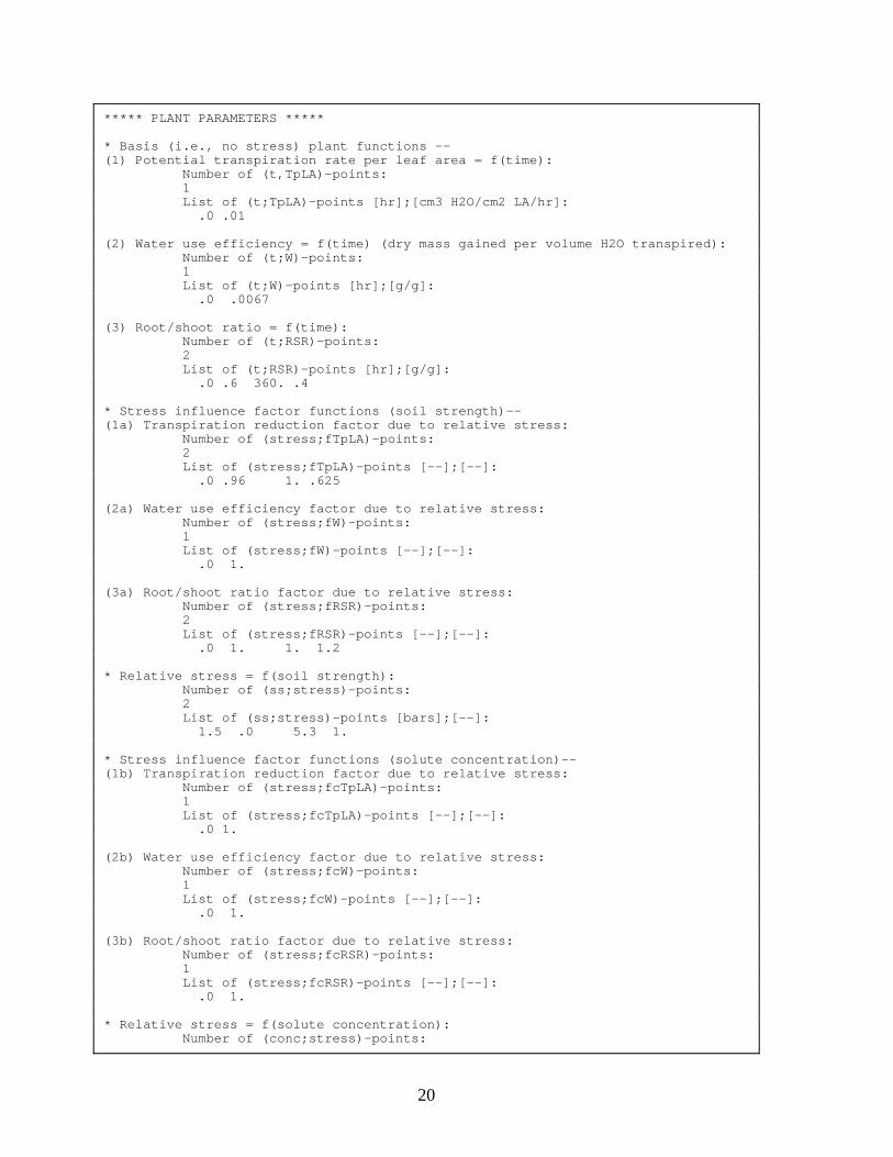
20

***** PLANT PARAMETERS ***** * Basis (i.e., no stress) plant functions -- (1) Potential transpiration rate per leaf area = f(time): Number of (t,TpLA)-points: 1 List of (t;TpLA)-points [hr];[cm3 H2O/cm2 LA/hr]: .0 .01 (2) Water use efficiency = f(time) (dry mass gained per volume H2O transpired): Number of (t;W)-points: 1 List of (t;W)-points [hr];[g/g]: .0 .0067 (3) Root/shoot ratio = f(time): Number of (t;RSR)-points: 2 List of (t;RSR)-points [hr];[g/g]: .0 .6 360. .4 * Stress influence factor functions (soil strength)-- (1a) Transpiration reduction factor due to relative stress: Number of (stress;fTpLA)-points: 2 List of (stress;fTpLA)-points [--];[--]: .0 .96 1. .625 (2a) Water use efficiency factor due to relative stress: Number of (stress;fW)-points: 1 List of (stress;fW)-points [--];[--]: .0 1. (3a) Root/shoot ratio factor due to relative stress: Number of (stress;fRSR)-points: 2 List of (stress;fRSR)-points [--];[--]: .0 1. 1. 1.2 * Relative stress = f(soil strength): Number of (ss;stress)-points: 2 List of (ss;stress)-points [bars];[--]: 1.5 .0 5.3 1. * Stress influence factor functions (solute concentration)-- (1b) Transpiration reduction factor due to relative stress: Number of (stress;fcTpLA)-points: 1 List of (stress;fcTpLA)-points [--];[--]: .0 1. (2b) Water use efficiency factor due to relative stress: Number of (stress;fcW)-points: 1 List of (stress;fcW)-points [--];[--]: .0 1. (3b) Root/shoot ratio factor due to relative stress: Number of (stress;fcRSR)-points: 1 List of (stress;fcRSR)-points [--];[--]: .0 1. * Relative stress = f(solute concentration): Number of (conc;stress)-points:

21

1 List of (conc;stress)-points [microMole/cm3];[--]: 0. 0. * Leaf area increase per increase in dry shoot mass: Number of (t;LA/mshoot)-points: 1 List of (t;LA/mshoot)-points [hr];[cm2/g]: .0 200.

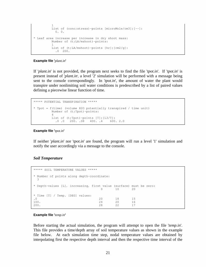
Example file 'plant.in' If 'plant.in' is not provided, the program next seeks to find the file 'tpot.in'. If 'tpot.in' is present instead of 'plant.in', a level '2' simulation will be performed with a message being sent to the console correspondingly. In 'tpot.in', the amount of water the plant would transpire under nonlimiting soil water conditions is predescribed by a list of paired values defining a piecewise linear function of time. ***** POTENTIAL TRANSPIRATION ***** * Tpot = f(time) (volume H2O potentially transpired / time unit) Number of (t;Tpot)-points: 4 List of (t;Tpot)-points [T];[L3/T]: .0 .0 200. .08 400. .4 600. 2.0

Example file 'tpot.in' If neither 'plant.in' nor 'tpot.in' are found, the program will run a level '1' simulation and notify the user accordingly via a message to the console. Soil Temperature ***** SOIL TEMPERATURE VALUES ***** * Number of points along depth-coordinate: 3 * Depth-values [L], increasing, first value (surface) must be zero: 0 10 20 * Time [T] / Temp. [DEG] values: .0 20 18 15 100. 24 20 16 200. 28 22 17

Example file 'temp.in' Before starting the actual simulation, the program will attempt to open the file 'temp.in'. This file provides a time/depth array of soil temperature values as shown in the example file below. At each simulation time step, nodal temperature values are obtained by interpolating first the respective depth interval and then the respective time interval of the

22

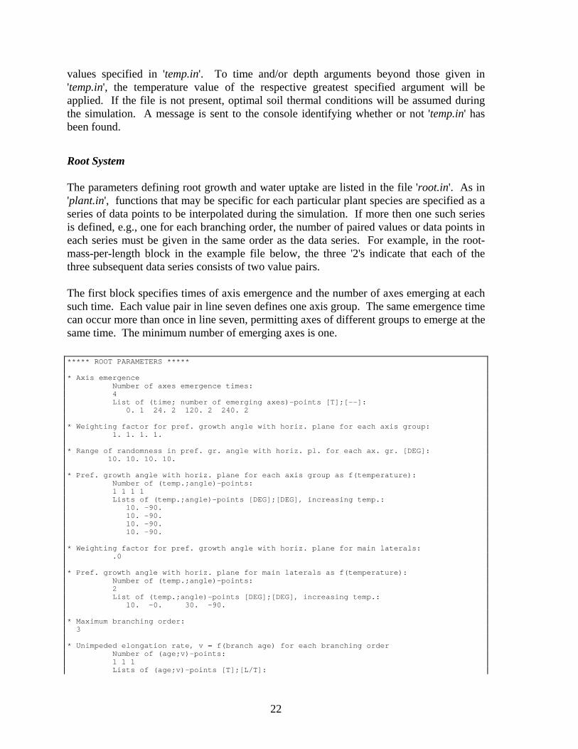
values specified in 'temp.in'. To time and/or depth arguments beyond those given in 'temp.in', the temperature value of the respective greatest specified argument will be applied. If the file is not present, optimal soil thermal conditions will be assumed during the simulation. A message is sent to the console identifying whether or not 'temp.in' has been found. Root System The parameters defining root growth and water uptake are listed in the file 'root.in'. As in 'plant.in', functions that may be specific for each particular plant species are specified as a series of data points to be interpolated during the simulation. If more then one such series is defined, e.g., one for each branching order, the number of paired values or data points in each series must be given in the same order as the data series. For example, in the root-mass-per-length block in the example file below, the three '2's indicate that each of the three subsequent data series consists of two value pairs. The first block specifies times of axis emergence and the number of axes emerging at each such time. Each value pair in line seven defines one axis group. The same emergence time can occur more than once in line seven, permitting axes of different groups to emerge at the same time. The minimum number of emerging axes is one. ***** ROOT PARAMETERS ***** * Axis emergence Number of axes emergence times: 4 List of (time; number of emerging axes)-points [T];[--]: 0. 1 24. 2 120. 2 240. 2 * Weighting factor for pref. growth angle with horiz. plane for each axis group: 1. 1. 1. 1. * Range of randomness in pref. gr. angle with horiz. pl. for each ax. gr. [DEG]: 10. 10. 10. 10. * Pref. growth angle with horiz. plane for each axis group as f(temperature): Number of (temp.;angle)-points: 1 1 1 1 Lists of (temp.;angle)-points [DEG];[DEG], increasing temp.: 10. -90. 10. -90. 10. -90. 10. -90. * Weighting factor for pref. growth angle with horiz. plane for main laterals: .0 * Pref. growth angle with horiz. plane for main laterals as f(temperature): Number of (temp.;angle)-points: 2 List of (temp.;angle)-points [DEG];[DEG], increasing temp.: 10. -0. 30. -90. * Maximum branching order: 3 * Unimpeded elongation rate, v = f(branch age) for each branching order Number of (age;v)-points: 1 1 1 Lists of (age;v)-points [T];[L/T]:

23

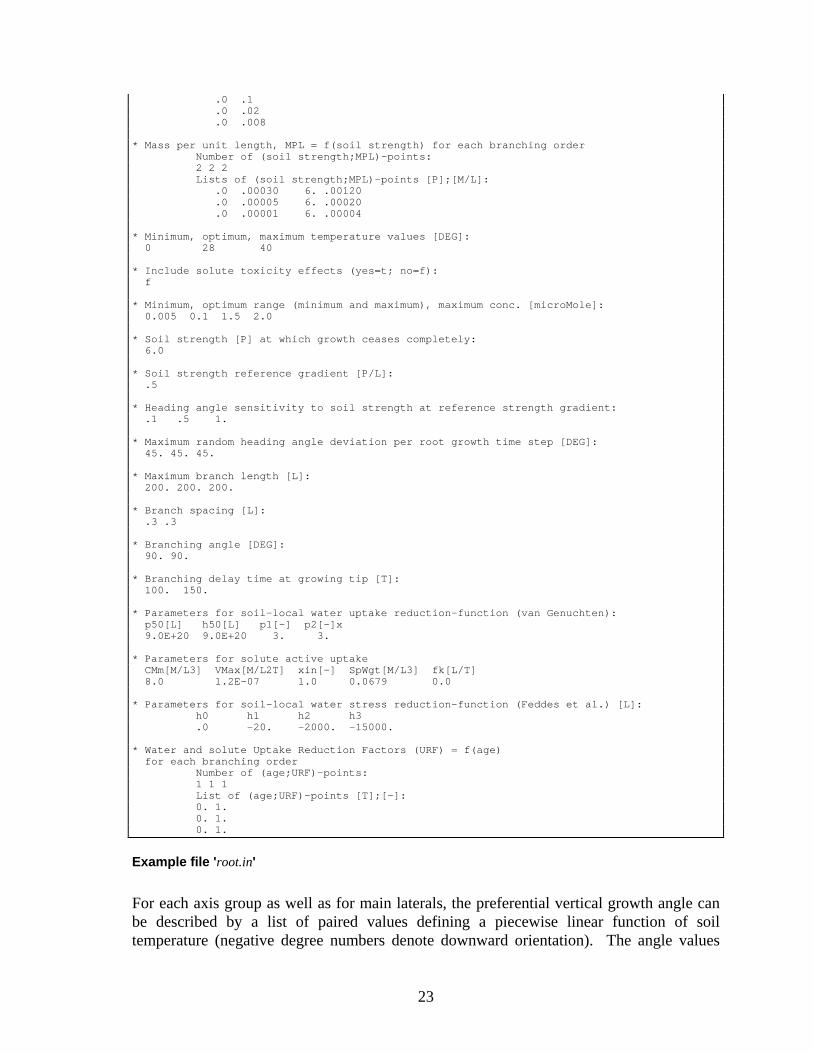
.0 .1 .0 .02 .0 .008 * Mass per unit length, MPL = f(soil strength) for each branching order Number of (soil strength;MPL)-points: 2 2 2 Lists of (soil strength;MPL)-points [P];[M/L]: .0 .00030 6. .00120 .0 .00005 6. .00020 .0 .00001 6. .00004 * Minimum, optimum, maximum temperature values [DEG]: 0 28 40 * Include solute toxicity effects (yes=t; no=f): f * Minimum, optimum range (minimum and maximum), maximum conc. [microMole]: 0.005 0.1 1.5 2.0 * Soil strength [P] at which growth ceases completely: 6.0 * Soil strength reference gradient [P/L]: .5 * Heading angle sensitivity to soil strength at reference strength gradient: .1 .5 1. * Maximum random heading angle deviation per root growth time step [DEG]: 45. 45. 45. * Maximum branch length [L]: 200. 200. 200. * Branch spacing [L]: .3 .3 * Branching angle [DEG]: 90. 90. * Branching delay time at growing tip [T]: 100. 150. * Parameters for soil-local water uptake reduction-function (van Genuchten): p50[L] h50[L] p1[-] p2[-]x 9.0E+20 9.0E+20 3. 3. * Parameters for solute active uptake CMm[M/L3] VMax[M/L2T] xin[-] SpWgt[M/L3] fk[L/T] 8.0 1.2E-07 1.0 0.0679 0.0 * Parameters for soil-local water stress reduction-function (Feddes et al.) [L]: h0 h1 h2 h3 .0 -20. -2000. -15000. * Water and solute Uptake Reduction Factors (URF) = f(age) for each branching order Number of (age;URF)-points: 1 1 1 List of (age;URF)-points [T];[-]: 0. 1. 0. 1. 0. 1.

Example file 'root.in'

For each axis group as well as for main laterals, the preferential vertical growth angle can be described by a list of paired values defining a piecewise linear function of soil temperature (negative degree numbers denote downward orientation). The angle values

24

assigned to the individual axes within each axis group will be equal to a random value deviating from the value specified for the group by up to ± ½ the group's range value in line 13. Whenever the new growth direction vector for the respective axis or main lateral is assembled, the weighting factor value will determine the relative importance of the preferential vertical growth angle component. A weighting factor of zero eliminates this component completely. The growth direction vector is explained in more detail in section VI. under subroutines nwcomp and geocom. The maximum branching order is set, and unimpeded elongation rate as a function of branch age and root mass per length as a function of soil strength are specified for each branching order by a list of paired values defining a piecewise linear function. In the following line, the minimum, optimum, maximum temperature values, necessary for the definition of the temperature impedance function are specified. If solution concentration effects on growth rate are taken into account at any of the six simulation levels, the user must indicate so in this section of the file. The four parameters needed for construction of the impedance function impc must be then specified, namely cmin, coptmin, coptmax, and cmax, with the second and third parameter defining the optimal concentration range. If this option is being considered but solute transport is not included at the designed simulation level, an initial solute concentration must be specified in the FEM input file. The heading angle sensitivity value is used as weighting factor together with the soil strength reference gradient in subroutine ssgcom to calculate the soil strength gradient component of the growth direction vector. This procedure is explained in section VI. Heading angle sensitivity, maximum random deviation, and maximum branch length are to be specified for each branching order. Branch spacing is defined as the distance between two subsequent subbranch origination points. The branching angle is the angle between branch and subbranch at the point where the subbranch originates; branching delay time is the minimum age for subbranch origination points. All three parameters are defined for the base branch's branching order, i.e., the parameters specified for branching order '1' will be used to determine initial time, position and angle for branches of order '2' originating from order '1'. The following three blocks contain the parameters defining the water and solute uptake functions: the parameters defining the water uptake reduction function α are specified in the first line (see eq. (12)); the second line lists the parameters needed for calculation of active solute uptake, namely: the Michaelis-Menten constant; the maximum uptake rate; the partition coefficient between passive and active uptake; the root specific dry weight (dry weight over bulk volume, from Silk et al., 1986), this last parameter being needed for computation of root surface area using segment mass and length; and last the first-order rate coefficient (see eq. (17)). If the parameter π50 is set equal to the dummy value '9.0E+20', then the function α is calculated according to eq. (13). If the parameter h50 is also set equal to the same dummy value, then the Feddes function is used (see Figure 2), using the parameters listed in the third line of the block.

25

In the last section of the file a set of weighting factors is listed as a function of age, in a sequence of paired values defining a piecewise linear function for each branching order. These factors are used in calculation of the root density functions β' and σ' needed for computation of the water and solute sink terms, to partially or totally exclude selected portions of root system from playing an active role in the uptake process. Time: 0.00000 Root DM, shoot DM, leaf area: 1.0E-05 1.0E-02 2. Average soil strength and solute concentration experienced by root system: 1.6 1.0 Total # of axes: 1 Total # of branches, including axis(es): 1 Total # of segment records: 1 segID# x y z prev or br# length surface mass origination time 1 0.000E+00 0.000E+00 4.000E+01 0 1 1 1.00E-04 0.0 0.0 0.0000E+00 total # of growing branch tips: 1 tipID# xg yg zg sg.bhd.tp. ord br# tot.br.lgth. axs# overlength # of estbl.d pts. time of establishing (-->) 1 0.0000E+00 0.0000E+00 3.9999E+01 1 1 1 1.0000E-04 1 -1. 0

Example file defining the initial root system The program will prompt the user for the name of the file describing the initial root system. Similar to the files containing the list of nodal values, root system output files of previous simulations can be used as input files for subsequent simulations. The top part of the file includes values applying to the whole system at the given time. It is followed by the list of individual segment records, each consisting of one line of parameter values, and the list of growing apices, each described by two lines of parameter values. The example in the following page is for a root consisting of only one segment with the respective apex, the smallest root "system" from which a growth simulation can be started. The values for shoot dry mass and leaf area will only be meaningful for level '3' simulations. They are stored with the root system information to avoid dealing with a specific file for these two values only. If a level '3' simulation is to be performed that begins immediately after germination, an initial leaf area greater than zero needs to be

26

specified so that the resulting photosynthate can serve as equivalent for the nutrition stored in the seed which is not considered by the model. The individual segment records consist of a global segment identification number, the spatial coordinates of the origination point of the segment (i.e., its "rear" end), the record number of the preceding segment, the branching order of the branch to which the segment belongs, segment length, surface and mass values, and the time at which the segment was originated. The information stored for each growing apex includes its identification number within the list of all growing apices, its position in space, the record number of the segment immediately behind the apex, the branching order of the branch to which the apex belongs, the total current length of that branch (i.e., the combined length of all segments between the apex and the branch origination point), the number of the axis to whose system the branch belongs, and, in subsequent lines, current values for the establishing of potential subbranch origination points behind the apex. The second line of numerical information for each apex includes the remainder of the last-applied branching distance and the total number of currently established potential subbranch origination points. Any times at which points have been established would be stored beginning in a third line. If the branch is only one segment long, the remainder value will show a negative number, indicating no "leftover" branching distance because there is no preceding segment within the same branch.

27

IV. MODEL OUTPUT AND POSTPROCESSING Simulation Record During each simulation, the program creates a file 'log'. The important time-varying parameters are recorded in this file by adding a new line with current values at each time step. Values for Tpot and Tact represent volumetric flow rates as defined in section II. The parameters grwfac and sAvg denote the assimilate allocation factor for root growth (explained under subroutine adjust in section VI.) and the average soil strength experienced by the root system, respectively. The last two columns show the development of shoot and root dry mass with simulation time. The example files demonstrate which parameters are recorded for each simulation level. Usually, the root dry mass value will not change with each new line because the FEM iterations can be expected to proceeded at time increments smaller than the user-specified root growth time steps. Time Tpot Tact grwfac sAvg cAvg mShoot mRoot 4.000E+00 n/a n/a n/a 1.600E+00 1.000E+00 n/a 1.000E-05 8.000E+00 n/a n/a n/a 1.600E+00 1.000E+00 n/a 1.000E-05 1.200E+01 n/a n/a n/a 1.631E+00 3.280E-02 n/a 1.493E-04 1.800E+01 n/a n/a n/a 1.631E+00 3.280E-02 n/a 1.493E-04 2.100E+01 n/a n/a n/a 1.631E+00 3.280E-02 n/a 1.493E-04

Time Tpot Tact grwfac sAvg cAvg mShoot mRoot 4.000E+00 1.600E-03 1.600E-03 n/a 1.600E+00 1.000E+00 n/a 1.000E-05 8.000E+00 3.200E-03 3.200E-03 n/a 1.600E+00 1.000E+00 n/a 1.000E-05 1.200E+01 4.800E-03 4.800E-03 n/a 1.631E+00 3.280E-02 n/a 1.493E-04 1.800E+01 7.200E-03 7.200E-03 n/a 1.631E+00 3.280E-02 n/a 1.493E-04 2.100E+01 8.400E-03 8.400E-03 n/a 1.631E+00 3.280E-02 n/a 1.493E-04

Time Tpot Tact grwfac sAvg cAvg mShoot mRoot 4.000E+00 1.902E-02 1.902E-02 0.000E+00 1.600E+00 1.000E+00 1.032E-02 1.000E-05 8.000E+00 1.963E-02 1.963E-02 0.000E+00 1.600E+00 1.000E+00 1.065E-02 1.000E-05 1.200E+01 2.026E-02 2.026E-02 1.427E+00 1.633E+00 6.092E-01 1.099E-02 4.243E-04 1.800E+01 2.084E-02 2.084E-02 1.427E+00 1.633E+00 6.092E-01 1.151E-02 4.243E-04 2.100E+01 2.184E-02 2.184E-02 1.427E+00 1.633E+00 6.092E-01 1.179E-02 4.243E-04

Top parts of example log files for level '1', '2', and '3' simulation, respectively Soil Water and Solute Status All FEM output files are named 'outfem.ext', where the extension (ext) takes on the current count number for the FEM outputs, e.g., the third FEM output file would be created as 'outfem.3'. The top part of each FEM output includes the user information from 'control.in' and the current total volume of soil water and solute within the considered domain, obtained from numerically integrating the volumetric soil water content and the concentration over the

28

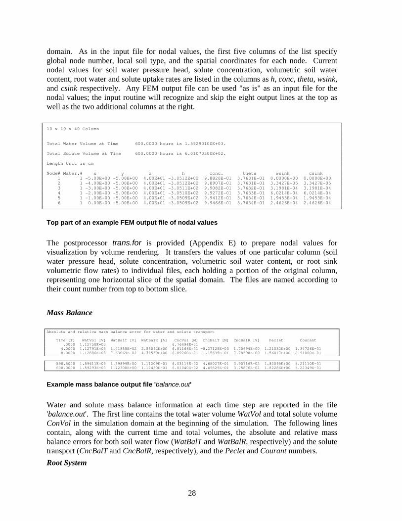
domain. As in the input file for nodal values, the first five columns of the list specify global node number, local soil type, and the spatial coordinates for each node. Current nodal values for soil water pressure head, solute concentration, volumetric soil water content, root water and solute uptake rates are listed in the columns as h, conc, theta, wsink, and csink respectively. Any FEM output file can be used "as is" as an input file for the nodal values; the input routine will recognize and skip the eight output lines at the top as well as the two additional columns at the right. 10 x 10 x 40 Column Total Water Volume at Time 600.0000 hours is 1.59290100E+03. Total Solute Volume at Time 600.0000 hours is 6.01070300E+02. Length Unit is cm Node# Mater.# x y z h conc. theta wsink csink 1 1 -5.00E+00 -5.00E+00 4.00E+01 -3.0512E+02 9.8820E-01 3.7631E-01 0.0000E+00 0.0000E+00 2 1 -4.00E+00 -5.00E+00 4.00E+01 -3.0512E+02 9.8907E-01 3.7631E-01 3.3427E-05 3.3427E-05 3 1 -3.00E+00 -5.00E+00 4.00E+01 -3.0511E+02 9.9082E-01 3.7632E-01 3.1981E-04 3.1981E-04 4 1 -2.00E+00 -5.00E+00 4.00E+01 -3.0510E+02 9.9272E-01 3.7633E-01 6.0214E-04 6.0214E-04 5 1 -1.00E+00 -5.00E+00 4.00E+01 -3.0509E+02 9.9412E-01 3.7634E-01 1.9453E-04 1.9453E-04 6 1 0.00E+00 -5.00E+00 4.00E+01 -3.0509E+02 9.9466E-01 3.7634E-01 2.4626E-04 2.4626E-04

Top part of an example FEM output file of nodal values The postprocessor trans.for is provided (Appendix E) to prepare nodal values for visualization by volume rendering. It transfers the values of one particular column (soil water pressure head, solute concentration, volumetric soil water content, or root sink volumetric flow rates) to individual files, each holding a portion of the original column, representing one horizontal slice of the spatial domain. The files are named according to their count number from top to bottom slice. Mass Balance Absolute and relative mass balance error for water and solute transport Time [T] WatVol [V] WatBalT [V] WatBalR [%] CncVol [M] CncBalT [M] CncBalR [%] Peclet Courant .0000 1.12750E+03 6.76494E+01 4.0000 1.12791E+03 1.41855E-02 2.55092E+00 6.81166E+01 -8.27125E-03 1.70694E+00 1.21032E+00 1.34726E-01 8.0000 1.12886E+03 7.63069E-02 4.78530E+00 6.89260E+01 -1.15835E-01 7.78698E+00 1.56017E+00 2.91000E-01 598.5000 1.59611E+03 1.39899E+00 1.11209E-01 6.03114E+02 4.65027E-01 3.90716E-02 1.82095E+00 5.21110E-01 600.0000 1.59293E+03 1.42300E+00 1.12430E-01 6.01040E+02 4.49829E-01 3.75876E-02 1.82286E+00 5.22349E-01

Example mass balance output file 'balance.out' Water and solute mass balance information at each time step are reported in the file 'balance.out'. The first line contains the total water volume WatVol and total solute volume ConVol in the simulation domain at the beginning of the simulation. The following lines contain, along with the current time and total volumes, the absolute and relative mass balance errors for both soil water flow (WatBalT and WatBalR, respectively) and the solute transport (CncBalT and CncBalR, respectively), and the Peclet and Courant numbers. Root System

29

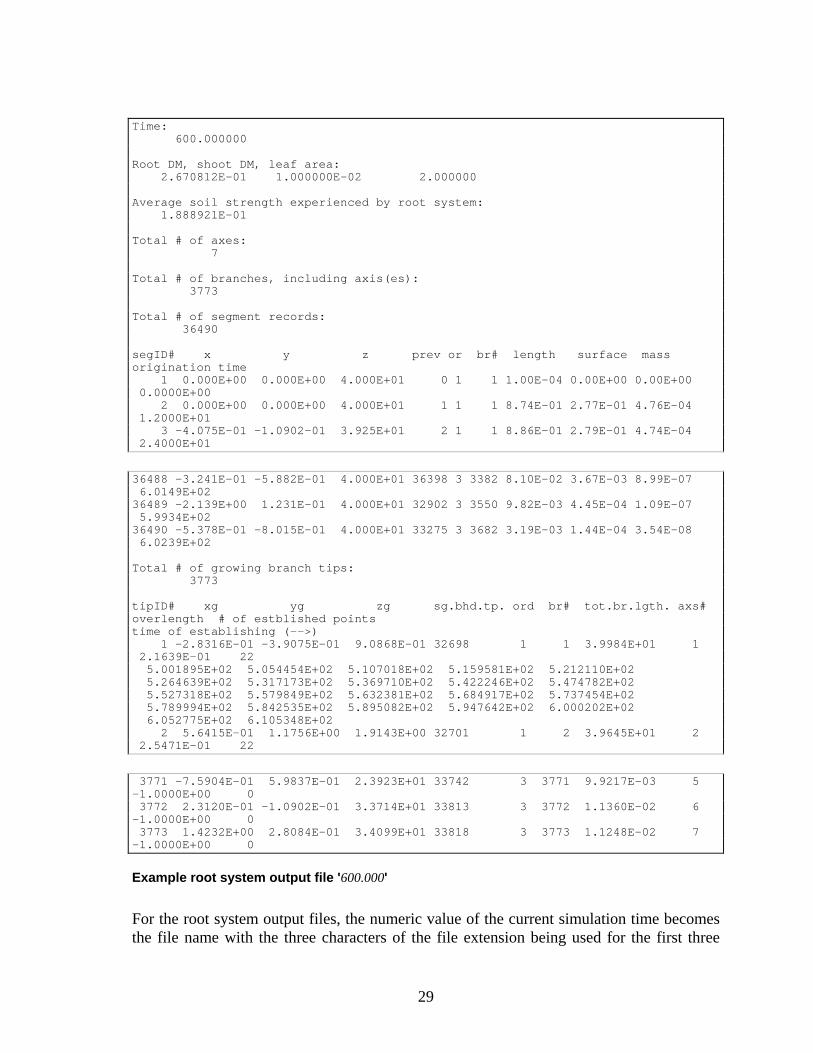
Time: 600.000000 Root DM, shoot DM, leaf area: 2.670812E-01 1.000000E-02 2.000000 Average soil strength experienced by root system: 1.888921E-01 Total # of axes: 7 Total # of branches, including axis(es): 3773 Total # of segment records: 36490 segID# x y z prev or br# length surface mass origination time 1 0.000E+00 0.000E+00 4.000E+01 0 1 1 1.00E-04 0.00E+00 0.00E+00 0.0000E+00 2 0.000E+00 0.000E+00 4.000E+01 1 1 1 8.74E-01 2.77E-01 4.76E-04 1.2000E+01 3 -4.075E-01 -1.0902-01 3.925E+01 2 1 1 8.86E-01 2.79E-01 4.74E-04 2.4000E+01

36488 -3.241E-01 -5.882E-01 4.000E+01 36398 3 3382 8.10E-02 3.67E-03 8.99E-07 6.0149E+02 36489 -2.139E+00 1.231E-01 4.000E+01 32902 3 3550 9.82E-03 4.45E-04 1.09E-07 5.9934E+02 36490 -5.378E-01 -8.015E-01 4.000E+01 33275 3 3682 3.19E-03 1.44E-04 3.54E-08 6.0239E+02 Total # of growing branch tips: 3773 tipID# xg yg zg sg.bhd.tp. ord br# tot.br.lgth. axs# overlength # of estblished points time of establishing (-->) 1 -2.8316E-01 -3.9075E-01 9.0868E-01 32698 1 1 3.9984E+01 1 2.1639E-01 22 5.001895E+02 5.054454E+02 5.107018E+02 5.159581E+02 5.212110E+02 5.264639E+02 5.317173E+02 5.369710E+02 5.422246E+02 5.474782E+02 5.527318E+02 5.579849E+02 5.632381E+02 5.684917E+02 5.737454E+02 5.789994E+02 5.842535E+02 5.895082E+02 5.947642E+02 6.000202E+02 6.052775E+02 6.105348E+02 2 5.6415E-01 1.1756E+00 1.9143E+00 32701 1 2 3.9645E+01 2 2.5471E-01 22

3771 -7.5904E-01 5.9837E-01 2.3923E+01 33742 3 3771 9.9217E-03 5 -1.0000E+00 0 3772 2.3120E-01 -1.0902E-01 3.3714E+01 33813 3 3772 1.1360E-02 6 -1.0000E+00 0 3773 1.4232E+00 2.8084E-01 3.4099E+01 33818 3 3773 1.1248E-02 7 -1.0000E+00 0

Example root system output file '600.000' For the root system output files, the numeric value of the current simulation time becomes the file name with the three characters of the file extension being used for the first three

30

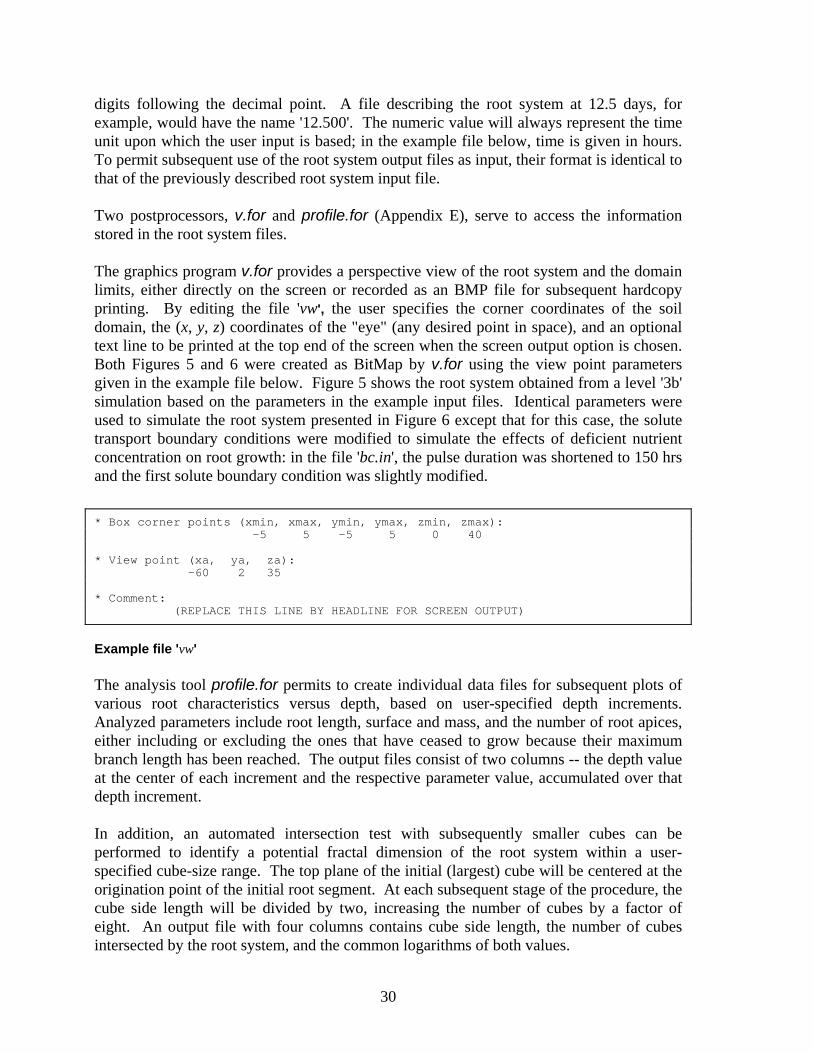
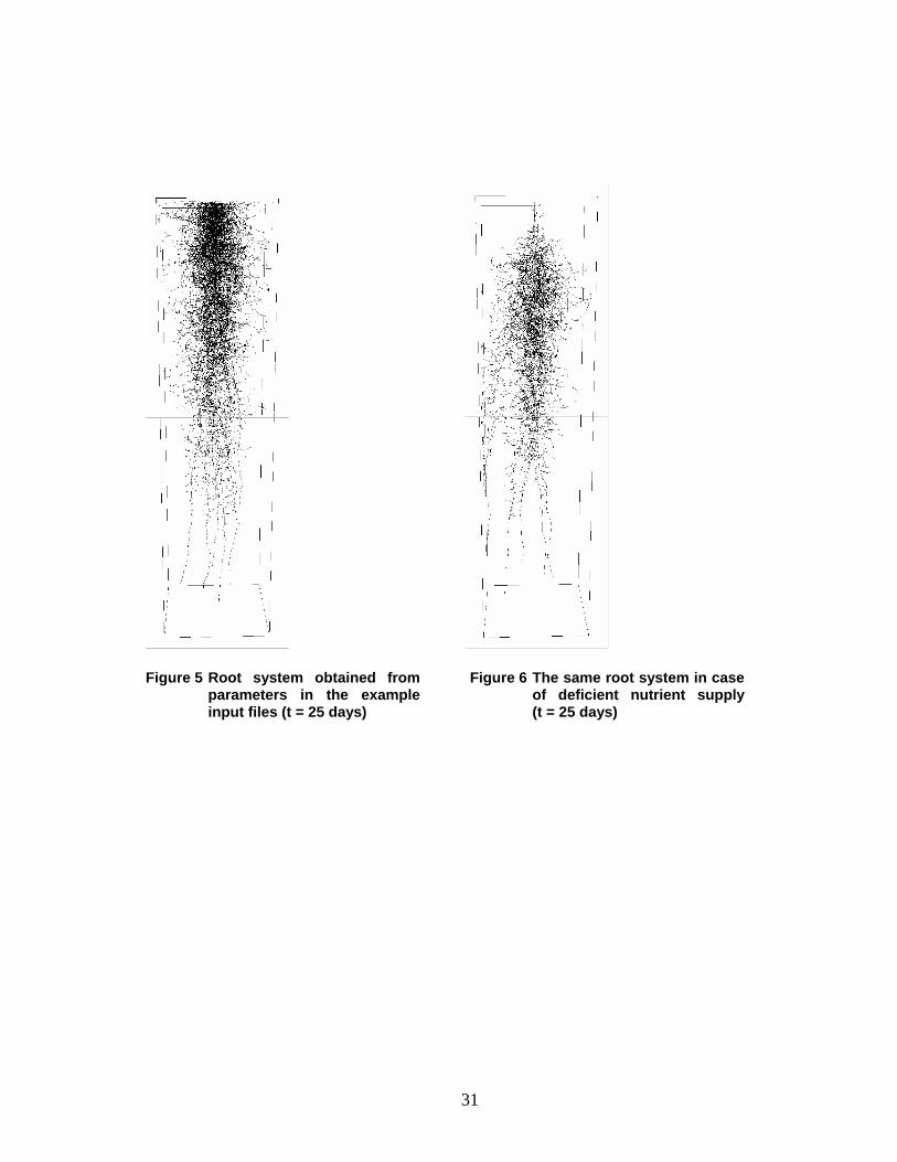
digits following the decimal point. A file describing the root system at 12.5 days, for example, would have the name '12.500'. The numeric value will always represent the time unit upon which the user input is based; in the example file below, time is given in hours. To permit subsequent use of the root system output files as input, their format is identical to that of the previously described root system input file. Two postprocessors, v.for and profile.for (Appendix E), serve to access the information stored in the root system files. The graphics program v.for provides a perspective view of the root system and the domain limits, either directly on the screen or recorded as an BMP file for subsequent hardcopy printing. By editing the file 'vw', the user specifies the corner coordinates of the soil domain, the (x, y, z) coordinates of the "eye" (any desired point in space), and an optional text line to be printed at the top end of the screen when the screen output option is chosen. Both Figures 5 and 6 were created as BitMap by v.for using the view point parameters given in the example file below. Figure 5 shows the root system obtained from a level '3b' simulation based on the parameters in the example input files. Identical parameters were used to simulate the root system presented in Figure 6 except that for this case, the solute transport boundary conditions were modified to simulate the effects of deficient nutrient concentration on root growth: in the file 'bc.in', the pulse duration was shortened to 150 hrs and the first solute boundary condition was slightly modified. * Box corner points (xmin, xmax, ymin, ymax, zmin, zmax): -5 5 -5 5 0 40 * View point (xa, ya, za): -60 2 35 * Comment: (REPLACE THIS LINE BY HEADLINE FOR SCREEN OUTPUT)

Example file 'vw' The analysis tool profile.for permits to create individual data files for subsequent plots of various root characteristics versus depth, based on user-specified depth increments. Analyzed parameters include root length, surface and mass, and the number of root apices, either including or excluding the ones that have ceased to grow because their maximum branch length has been reached. The output files consist of two columns -- the depth value at the center of each increment and the respective parameter value, accumulated over that depth increment. In addition, an automated intersection test with subsequently smaller cubes can be performed to identify a potential fractal dimension of the root system within a user-specified cube-size range. The top plane of the initial (largest) cube will be centered at the origination point of the initial root segment. At each subsequent stage of the procedure, the cube side length will be divided by two, increasing the number of cubes by a factor of eight. An output file with four columns contains cube side length, the number of cubes intersected by the root system, and the common logarithms of both values.

31

Figure 5 Root system obtained from

parameters in the example input files (t = 25 days)

Figure 6 The same root system in case of deficient nutrient supply (t = 25 days)

32

V. HARDWARE AND SOFTWARE REQUIREMENTS The size of the problem to be modeled is limited by the available random-access memory (RAM). Memory size and computing speed make workstations the preferred hardware choice. However, personal computers as the less expensive alternative are, of course, still much more widely distributed. Using a PC - Both the root system and the finite element grid being memory-intense structures, it can be expected that virtually every application of the model will require more than the 640 Kbytes commonly available under DOS. It is recommended that the program be executed with at least 8 Mbyte RAM installed. The FORTRAN system used must give access to all of the installed RAM. Possible choices include the FTN77/386 or FTN77/486 by the University of Salford1 and the Microsoft FORTRAN Powerstation. Any DOS-only FORTRAN, in contrast, is limited to 640 Kbyte. Portability - Being based almost exclusively on the FORTRAN77 standard, easy portability of the model source code is ensured. The source code as provided is written for Microsoft FORTRAN Powerstation. The presumably only exceptions to complete portability are (1), the random number generator for which no standard exists and (2), the POSITION='APPEND' option under which the log file is opened in log and the mass balance file is opened in subreg. When porting to a different FORTRAN system, the statements for initializing and executing the random number generator as well as for specifying the 'APPEND' mode may have to be replaced. In Microsoft FORTRAN Powerstation, the sequence of random numbers is initialized by a keyboard input of the random number generator seed and then CALL srand; subsequent members of the sequence are obtained using the rand(0)-function. Unlike the previous version of the program, therefore, it is possible to test the effects of different inputs on the very same root system by specifying the same random number generator seed at the beginning of the simulation. The program has been successfully tested for both Microsoft FORTRAN Powerstation on a PC and VAX FORTRAN on DEC workstations (DEC 3100 and DEC 5000). Graphics - Visualizing either part of or the complete set of nodal pressure head, solute concentrations, water content, or water and solute uptake rate values in the FEM output file requires a software capable of rendering volume data. For example, SLICER for Windows2 software offers both grey shading and color tables for 3D data. The program trans.for or the appropriate NCSA-HDF3 subroutines (NCSA-HDF, University of Illinois at Urbana-Champaign, public domain) can be used to extract the desired data from a FEM output file, creating SLICER input files. Three dimensional data sets can be extracted from a FEM output file simply using Microsoft EXCEL. HDF files can also be used as input to the 4d2

1Salford Software Marketing Ltd, Bridgewater Buliding, Univ. of Salford, Salford M5 4WT, U.K. 2Fortner Research LLC, 100 Carpenter Dr, Sterling, VA 20164; (703) 689-9593

33

software package3 (NCSA, University of Illinois at Urbana-Champaign, public domain) for three-dimensional time animation on UNIX systems. The graphics postprocessor for the root system, v.for, has been specifically written for Microsoft FORTRAN Powerstation. Screen graphics is created for High-Resolution VGA. The bitmap graphics files for hardcopies will match a 300 DPI resolution on laser printers. Any software that is compatible with the bitmap format (for example, Microsoft Paint or CorelPHOTO-PAINT4) can be used to print the hardcopies. If a different FORTRAN package is to be used, some of the graphics subroutines in v.for will have to be replaced by their respective counterparts from that package. The comment lines in the graphics postprocessor source code should provide ample guidance for necessary module replacements. The ASCII data files created by profile.for can be plotted using any suitable spreadsheet software.

3 NCSA Software Development-HDF, 152 Computing Application Building, 605 Springfield Avenue, Champaign, IL 61820 4 Corel Corporation, P.O. Box 3595, Salinas, CA 93912-3595; (613) 728-8200

34

VI. PROGRAM STRUCTURE AND VARIABLES USED Principal Design The principal designs of the main program and its three main subroutines, WATER, SOLUTE and ROOT, are depicted by the charts 1, 2, 3 and 4, respectively, in the following three pages. The subsequent main part of this section covers the subroutines and functions of the current version of the program. For enhanced readability, most variables have been organized in COMMON blocks. A reference list including the names, types, and meanings of the variables assigned to each block is provided as Appendix B. Array size is assigned by PARAMETER-statements and can thus be quickly changed in the source code using the replace-command which any text editor should provide. PARAMETER Definition: maximum permitted number of... maxaxs maxbdr maxbnd maxelm maxemg maxest maxgrw maxmat maxnod maxord maxrec mxofem mxoroo mxpnts mxbcch mxdpth mxtime ntab

root axes nodes for which boundary conditions have been specified bandwidth size elements making up the FEM grid axis group emergence events potential branching points behind a growing apex simultaneously growing apices different soil types within domain nodes making up the FEM grid branching orders root segment records FEM output events root system output events points making up a stepwise-linear input function points making up a stepwise-linear input or B.C. function depth values for which stepwise-linear soil temperature = f(time) is specified time values for which soil temperature values are specified tabulated (soil water pressure head, conductivity, capacity)-triplets for each soil type

Table 2. Names and definitions of the PARAMETER variables.

35

MAIN PROGRAM call to subroutine

input applic chemin soilin rootin plntin tempin

initial root and root surface distribution functions betdis normalize root distribution functions betnrm obtain current soil hydraulic properties setmat initialize transport parameters chinit initialize water and solute mass balance variables subreg

begin time loop

adjust time step length tmcont current relative stress stress ⇓_ bypass for level '1' or

'2' simulations current potential transpiration rate settp current B.C.'s setbc set up FEM sink term array setsnk

obtain new pressure head profile WATER

if solute transport considered, obtain new concentration profile SOLUTE calculate water and solute mass balance subreg

actual transpiration rate acttrs ⇓_ bypass for level '1'

new biomass effncy ⇓ bypass for level '1' partition between root and shoot ratio ⇓ or '2' simulations root assimilate is accumulated until next root growth step ⇓ increase leaf area leaves ⇓_

if time matches "next root growth" time

current soil strength distribution solstr if temperature input is provided, update soil temp. profile temper if included, calculate inpedance-due-to-concentration factor contox let root system grow ROOT update "next root growth" time update root and root surface distribution functions betdis normalize root distribution functions betnrm

endif

write current plant parameters to log file log

if time matches "next FEM output" time, write FEM output file and update "next FEM output" time

outfem

if time matches "next root output" time, write root output file and update "next root output" time

outroo

end of simulation? getout

end time loop

Chart 1. Principal sequence of program modules.

36

SUBROUTINE WATER call to subroutine

begin FEM iteration loop for water flow

obtain current soil hydraulic properties setmat set up FEM matrix for water flow reset apply constant-head B.C.'s dirich solve FEM matrix solve test for convergence test for convergence

end FEM iteration loop

set up water mass balance watinf

return to MAIN

Chart 2. Sequence of modules for water flow.

SUBROUTINE SOLUTE call to subroutine

calculate nodal velocities veloc calculate nodal components of dispersivity tensor disper set up FEM matrix for solute transport apply constant concentration B.C.'s cbound solve FEM matrix solvet set up solute mass balance solinf

return to MAIN

Chart 3. Sequence of modules for solute transport.

37

SUBROUTINE ROOT call to subroutine

if time matches "next axes emergence" time, originate new axes and update "next axes emergence" time

newaxs

begin first apex loop

originate new subbranches at all branching points that have minimum age

brdevl

identify grid points surrounding apex neighb local soil strength at apex strloc branch age brnage new growth direction and tentative segment length

('tentative' because at this stage, only the local soil strength is controlling root elongation)

nwcomp

tentative segment mass maslen create new segment record mkrecd grow to new apex position grow

end first apex loop

update total mass of root system

calculate root allocation factor from accumulated root assimilate and tentative total new root mass

⇓ bypass for level '1' ⇓ or '2' simulations

reset accumulated root assimilate to zero ⇓_

begin second apex loop

adjust new growth using the allocation factor adjust ⇓ bypass for level '1' ⇓_ or '2' simulations

calculate subbranch distance spacng establish future subbranch origination points establ

end second apex loop

to prevent numerical problems, remove all new segments that are insignificantly small (e.g., smaller than ε = 1.E-6)

remove

begin third apex loop

enforce physical domain limits boxlim make a final record showing zero segment length for

branches that have reached maximum length mkrecd

end third apex loop

remove branches that have reached maximum length from list of growing branches

update

return to MAIN Chart 4. Principal sequence of modules for root growth simulation.

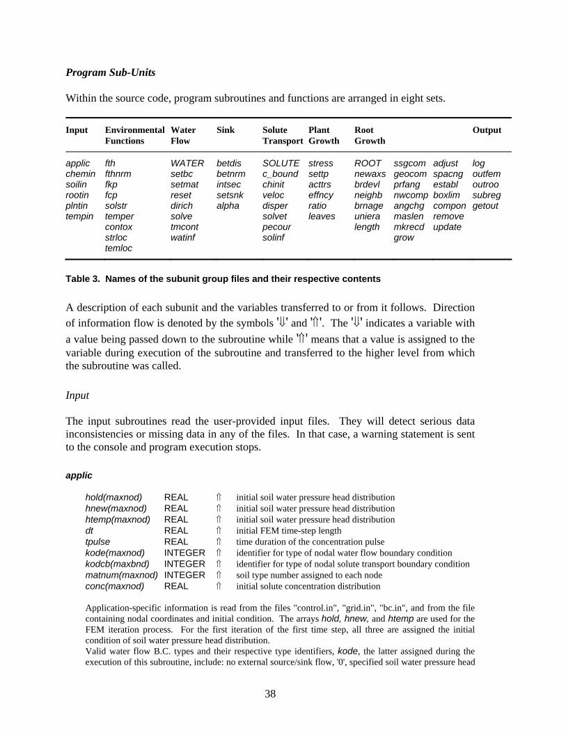
38

Program Sub-Units Within the source code, program subroutines and functions are arranged in eight sets. Input Environmental

Functions Water Flow

Sink Solute Transport

Plant Growth

Root Growth

Output

applic chemin soilin rootin plntin tempin

fth fthnrm fkp fcp solstr temper contox strloc temloc

WATER setbc setmat reset dirich solve tmcont watinf

betdis betnrm intsec setsnk alpha

SOLUTE c_bound chinit veloc disper solvet pecour solinf

stress settp acttrs effncy ratio leaves

ROOT newaxs brdevl neighb brnage uniera length

ssgcom geocom prfang nwcomp angchg maslen mkrecd grow

adjust spacng establ boxlim compon remove update

log outfem outroo subreg getout

Table 3. Names of the subunit group files and their respective contents

A description of each subunit and the variables transferred to or from it follows. Direction of information flow is denoted by the symbols '⇓' and '⇑'. The '⇓' indicates a variable with a value being passed down to the subroutine while '⇑' means that a value is assigned to the variable during execution of the subroutine and transferred to the higher level from which the subroutine was called. Input The input subroutines read the user-provided input files. They will detect serious data inconsistencies or missing data in any of the files. In that case, a warning statement is sent to the console and program execution stops. applic

hold(maxnod) hnew(maxnod) htemp(maxnod) dt tpulse kode(maxnod) kodcb(maxbnd) matnum(maxnod) conc(maxnod)

REAL REAL REAL REAL REAL INTEGER INTEGER INTEGER REAL

⇑ ⇑ ⇑ ⇑ ⇑ ⇑ ⇑ ⇑ ⇑

initial soil water pressure head distribution initial soil water pressure head distribution initial soil water pressure head distribution initial FEM time-step length time duration of the concentration pulse identifier for type of nodal water flow boundary condition identifier for type of nodal solute transport boundary condition soil type number assigned to each node initial solute concentration distribution

Application-specific information is read from the files "control.in", "grid.in", "bc.in", and from the file containing nodal coordinates and initial condition. The arrays hold, hnew, and htemp are used for the FEM iteration process. For the first iteration of the first time step, all three are assigned the initial condition of soil water pressure head distribution. Valid water flow B.C. types and their respective type identifiers, kode, the latter assigned during the execution of this subroutine, include: no external source/sink flow, '0', specified soil water pressure head

39

as a function of time, '+1', specified flux as a function of time, '-1', and free drainage, '-2'. For solute transport, the identifier kodcb is read from the file "bc.in". Valid B.C. types include: no external source/sink flow (no identifier assigned to those nodes), specified solute concentration as a function of time (first-type B.C., identifier has a positive sign), and specified flux as a function of time (second- and third-type B.C., identifier has a negative sign).

chemin

lchem LOGICAL ⇑ flag indicating whether or not solute transport is being considered

A set of transport parameters is read from the file "chem.in" for each of the soil types present in the domain, as well as the time weighing factor to use for approximation of the time derivatives in the solute transport equation and the parameter used as stability criterion for the solute transport scheme. If the file is not present in the current directory, lchem is set to FALSE and solute transport is not considered.

soilin

Parameters describing each soil type within the modeled domain are read and an interpolation table for each soil type's soil hydraulic conductivity and soil water capacity functions is created (COMMON /table/). Due to the involved floating-point operations in fkp and fcp, using the interpolation table during the FEM iterations results in faster program execution than direct evaluation of the hydraulic functions (Vogel, 1987).

rootin

naxes norder t mroot mshoot LA savg cavg toxi

INTEGER INTEGER REAL REAL REAL REAL REAL REAL LOGICAL

⇑ ⇑ ⇑ ⇑ ⇑ ⇑ ⇑ ⇑ ⇑

number of root axes present at time t maximum branching order for this species time associated with root system mass of root system at time t mass of shoot at time t leaf area at time t average soil strength felt by root apices at time t average solute concentration felt by root system at time t flag indicating whether or not concentration effects on growth are being considered

The files specifying the initial root system and the root growth and uptake parameters are read. The time associated with the initial root system will be the starting time for the simulation.

plntin

level lchem toxi

INTEGER LOGICAL LOGICAL

⇑ ⇓ ⇓

simulation level set to .TRUE. if solute transport is being considered set to .TRUE. if solute concentration effects on growth are included

This module first attempts to open file "plant.in", describing shoot function response to stress. If this information is provided, level is set equal to '3'. If "plant.in" is not present in the directory from which the program was started, plntin next looks for "tpot.in", containing a predefined function of potential transpiration over time. With "tpot.in" present instead of "plant.in", shoot growth and assimilate distribution will not be simulated, and level is set equal to '2'. If neither of the two files is provided, the

40

simulation will proceed ignoring both shoot function and root water and solute uptake and level is set equal to '1'.

tempin

temp LOGICAL ⇑ flag indicating whether soil temperature values are provided or not

The subroutine attempts to read soil temperature data from the file "temp.in". If this file is not present in the current directory, temp is set to FALSE and optimum temperature conditions are assumed during the simulation.

Environmental Functions This group contains functions for direct evaluation of soil hydraulic properties and subroutines to calculate both the current overall spatial distributions and local (i.e., in the vicinity of a particular root segment or apex) values of soil strength and soil temperature. The nodal values of impedance due to soil strength, soil temperature and nutrient concentration are calculated as well. fth

h par(15) fth

REAL REAL REAL

⇓ ⇓ ⇑

argument: soil water pressure head value soil type parameters volumetric soil water content, θ

fthnrm

h par(15) fthnrm

REAL REAL REAL

⇓ ⇓ ⇑

argument: soil water pressure head value soil type parameters normalized volumetric soil water content, Θ

fkp

h par(15) fkp

REAL REAL REAL

⇓ ⇓ ⇑

argument: soil water pressure head value soil type parameters hydraulic conductivity

fcp

h par(15) fcp

REAL REAL REAL

⇓ ⇓ ⇑

argument: soil water pressure head value soil type parameters soil water capacity

solstr

h(maxnod) matnum(maxnod)

REAL INTEGER

⇓ ⇓

current soil water pressure head distribution nodal soil type numbers

The current nodal soil strength and root-impedance-due-to-soil-strength values are calculated and stored as s(maxnod) and imps(maxnod), respectively, in the COMMON block /strgth/.

41

temper

t REAL ⇓ current simulation time

The current nodal soil temperature and root-impedance-due-to-soil-temperature values are calculated and stored as tem(maxnod) and impt(maxnod), respectively, in the COMMON block /tmptre/.

contox

conc(maxnod) REAL ⇓ current nodal concentration values as obtained from solving the FEM system of equations

This subroutine calculates the nodal values of the solute concentration impedance factor and stores them as impc(maxnod) in the COMMON block /conimp/.

strloc

corner(8) sloc

INTEGER REAL

⇓ ⇑

global node numbers of the 8 corner nodes of tip-containing cuboid average of the current soil strength values of the 8 corner nodes

Calculates the average soil strength value of each cuboid element.

temloc

temp corner(8) tloc

LOGICAL INTEGER REAL

⇓ ⇓ ⇑

set to .TRUE. if temperature data are provided global node numbers of the 8 corner nodes of tip-containing cuboid average of the current soil temperature values of the 8 corner nodes

Calculates the average temperature value of each cuboid element.

Water Flow The subroutines of this group set up and iteratively solve the system of equations for water flow at each FEM time step. They are partially modified units from Version 0.1 of SWM_3D by T. Vogel, 1990/91 (unpublished), an extension of the SWM II code (Vogel, 1987). All subroutines in this group other than WATER are being called during the execution of subroutine WATER.

42

WATER

hnew(maxnod) hold(maxnod) htemp(maxnod) t dt dtopt told matnum(maxnod) kode(maxnod) iter redo

REAL REAL REAL REAL REAL REAL REAL INTEGER INTEGER INTEGER LOGICAL

⇓ ⇑ ⇓ ⇓ ⇑ ⇓ ⇑ ⇓ ⇑ ⇓ ⇑ ⇓ ⇓ ⇓ ⇓ ⇑ ⇑

nodal soil water pressure head values as obtained from solving the FEM system of equations nodal soil water pressure head values at previous time step auxiliary array for nodal soil water pressure head values during the iteration process current simulation time time step length time step length, adjusted for convergence behavior current time at the last FEM iteration nodal soil type numbers identifier for type of nodal water flow boundary condition total number of iteration during the current time step set to .TRUE. if convergence has not been reached within the maximum permitted number of time steps

This is one of the three master subroutines, called from the main program at each time step. From here calls are made iteratively to each of the subroutines setting up the FEM matrix, imposing boundary conditions and solving the system of equations until the change in pressure head at the current and previous iteration satisfy the convergence criterion epslon set at the input. If convergence is not reached within the maximum number of iterations permitted, the time step is decreased at the main program and this module is called up again until convergence is reached or until the time step becomes smaller than the minimum time step allowed. In that case, a message is sent to the console warning the user, and the program stops. The sequence of subroutines in the WATER module is presented in chart 2, at the beginning of this section.

setbc

t h(maxnod) kode(maxnod)

REAL REAL INTEGER

⇓ ⇓ ⇑ ⇓

current simulation time nodal soil water pressure head values identifier for type of nodal water flow boundary condition

If defined, current head, concentration, and/or water and solute flow rate B.C. values are obtained from interpolating their respective input time-functions. Water flow B.C. are assigned to the boundary nodes during the execution of this subroutine: nodes with kode = +1 are subject to the head B.C., those with kode = -1 to the water flow rate B.C. Solute transport B.C. values are assigned to boundary nodes in the subroutine c_bound.

setmat

hold(maxnod) htemp(maxnod) hnew(maxnod) matnum(maxnod)

REAL REAL REAL INTEGER

⇓ ⇓ ⇓ ⇓

nodal soil water pressure head values at beginning of time step auxiliary array for nodal soil water pressure head values during the iteration process nodal soil water pressure head values as obtained from solving the FEM system of equations nodal soil type numbers

For each FEM iteration, nodal soil hydraulic conductivity and soil water capacity values are obtained according to nodal soil water pressure head values by interpolating the table of head, conductivity, and capacity values that was created in soilin as COMMON /table/. For head values outside the tabulated range, the hydraulic functions are evaluated directly by calling fkp and fcp. The old and current nodal

43

conductivity and capacity values are stored as cono(maxnod), con(maxnod) and cap(maxnod), respectively, in the COMMON block /concap/.

reset

kode(maxnod) hnew(maxnod) hold(maxnod) dt

INTEGER REAL REAL REAL

⇓ ⇓ ⇓ ⇓

identifier for type of nodal water flow boundary condition nodal soil water pressure head values as obtained from solving the FEM system of equations nodal soil water pressure head values at beginning of time step current time step length

This module performs the three-dimensional FEM integration of the water flow equation for each element and assembles the resulting system of linear equations which is stored as a(maxbnd, maxnod) and b(maxnod), respectively, in the COMMON block /matrix/.

dirich

kode(maxnod) hnew(maxnod)

INTEGER REAL

⇓ ⇓

identifier for type of nodal water flow boundary condition nodal soil water pressure head values as obtained from solving the FEM system of equations

If any, nodal constant-head B.C.'s are applied to the system of nonlinear equations in the COMMON block /matrix/.

solve

The system of linear equations in the COMMON block /matrix/ is solved with the solution being stored in b(maxnod).

tmcont

iter t dt dtopt tcallr tfem troo dtmaxc

INTEGER REAL REAL REAL REAL REAL REAL REAL

⇓ ⇓ ⇓ ⇑ ⇓ ⇑ ⇓ ⇓ ⇓ ⇓

total number of iterations during last time step current simulation time time step length time step length, adjusted for convergence behavior next time at which ROOT will be called next FEM output time next root-system output time maximum permitted time increment for solute transport

Time step length for the FEM procedures is increased by the factor facinc if iter ≤ 3 and decreased by facdec if iter ≥ 7. The adjustment factors are part of the COMMON block /tmctrl/. Before dt is returned to the main program, it is adjusted so that the maximum permitted time increment for solute transport is not exceeded (dt ≤ dtmaxc) and the prespecified times of upcoming output events or calls to ROOT will be matched. A further adjustment is also made so that dtmin<dt<dtmax .

watinf

kode(maxnod) dt

INTEGER REAL

⇓ ⇓

identifier for type of nodal water flow boundary condition time step length

44

Computes the sum of all cumulative water fluxes across the boundary surface, including internal sources or sinks, as well as the sum of their absolute values. These values will be used to set up the water mass balance and compute the absolute and relative mass balance errors.

Sink Current soil water pressure head, osmotic potential and root distributions as well as potential transpiration are translated into nodal sink values for the soil water flow FEM scheme. Active and passive uptake, the former being calculated using the Michaelis-Menten expression and the latter being obtained from the root water uptake, are summed up into nodal sink values for the solute transport FEM scheme. betdis

t REAL ⇓ current simulation time

This module assembles the current root distribution function betaw(maxnod) and rooting density function betac(maxnod) in COMMON block /uptake/. For each root segment, the eight nodes of the cuboid-element surrounding the segment originating point are identified via a call to neighb. A call to the logical function intersec determines whether or not the segment lies entirely within the cuboid-element. If it does, the eight nodal values of the betaw and betac functions are increased according to the reciprocal squared distance between the segment central point and the node, the segment age and: 1) the segment length for the betaw function or: 2) the segment surface for the betac function. If the segment spans several cuboid-elements, they are all identified and the betaw and betac functions of their respective nodes increased according to the position, age, and length or surface of the pertaining segment portion.

betnrm

After completed assembly, the current root distribution functions betaw(maxnod) and betac(maxnod) in COMMON block /uptake/ are normalized so that their volumetric integral over the soil domain is equal to unity.

intersec

xa,ya,za xb,yb,zb x1,y1,z1 x2,y2,z2 xint,yint,zint iface intersec

REAL REAL REAL INTEGER LOGICAL

⇓ ⇓ ⇑ ⇑ ⇑

x-, y- and z-coordinate of each segment origination and end point respectively maximum and minimum x-, y- and z-coordinate of the cuboid containing the segment origination point x-, y- and z-coordinate of the segment intersection point identifier for the cuboid-element's face to which the intersection point belongs flag indicating whether the segment intersects any of the cuboid-element's faces

This function checks for intersections between the root segment and the cuboid containing its origination point. If the test for intersection is positive, the coordinates of the intersection point are calculated.

45

setsnk

hnew(maxnod) conc(maxnod) tpot

REAL REAL REAL

⇓ ⇓ ⇓

nodal soil water pressure head values at the current time step nodal solute concentration values at the current time step current potential transpiration

For each node, a water uptake-reduction value alpha is obtained by calling the alpha-function with the current nodal values of soil water pressure head, solute concentration and temperature as argument. The nodal sink term for the water flow FEM scheme is calculated by multiplying the plant potential transpiration with the nodal alpha and betaw(maxnod) values. If active solute uptake is being considered, nodal values of the Michaelis-Menten expression are evaluated, multiplying the betac function with the total root surface to obtain the nodal root surface density. The nodal sink term for the solute transport FEM scheme is thus calculated adding the active and passive portion of uptake (the latter derived from the water uptake term) through the partition coefficient xin. The sink term arrays for water flow and solute transport FEM schemes are stored as sink(maxnod) and csink(maxnod) respectively, in COMMON block /uptake/.

alpha

h conc tem alpha

REAL REAL REAL REAL

⇓ ⇓ ⇓ ⇑

argument: soil water pressure head value argument: concentration value argument: temperature value uptake-reduction value

This function determines the nodal uptake-reduction value alpha using the parameters in COMMON block /extrct/. The option is provided to account for the combined effects of pressure and osmotic potential (van Genuchten and Gupta, 1993) or to consider the pressure effects only. In the latter case the van Genuchten's expression can be used, or the one by Feddes (1978). The user must verify the consistency of units between the variables provided as input and the conversion factors used in this module for calculation of the osmotic pressure prior to running the program.

Solute Transport The subroutines in this group set up and solve the system of equations for solute transport at each time step. Each of the units is a 3-D expansion of Version 1.1 of the SWMS_2D code (S

vimu°nek et al., 1992). All subroutines in this group other than SOLUTE and chinit

are being called during the execution of the subroutine SOLUTE. SOLUTE

dt t conc(maxnod) tpulse hold(maxnod) hnew(maxnod) dtmaxc matnum(maxnod) kode(maxnod) kodcb(maxbnd)

REAL REAL REAL REAL REAL REAL REAL INTEGER INTEGER INTEGER

⇓ ⇓ ⇓ ⇑ ⇓ ⇓ ⇓ ⇓ ⇓ ⇓ ⇓

current time step length current simulation time nodal concentration values as obtained from solving the FEM system of equations time duration of concentration pulse nodal soil water pressure head values at the previous time step nodal soil water pressure head values at the current time step maximum permitted time increment for solute transport nodal soil type number identifier for type of nodal water flow boundary condition identifier for type of nodal solute transport boundary condition

46

This is the second of the three master subroutines, called from the main program at each time step if solute transport is being considered. From this module, the nodal components of the Darcian velocity vector are obtained via a call to veloc and stored in the COMMON block /veloct/. These values will be used for calculation of the nodal components of the dispersivity tensor (stored in the COMMON block /disten/) via a call to disper. Three-dimensional FEM integration is performed over each element and the resulting system of linear equations is assembled and stored as the coefficient matrix a(maxbnd, maxnod) and the right-hand side vector b(maxnod) in the COMMON block /matrix/. Nodal boundary conditions are imposed by calling c_bound and the system of linear equations solved via a call to solvet. For the sequence of subroutine calls making up the SOLUTE module, refer to chart 3 at the beginning of this section.

c_bound

kode(maxnod) kodcb(maxbnd) conc(maxnod) dt ds(maxnod)

INTEGER INTEGER REAL REAL REAL

⇓ ⇓ ⇓ ⇑ ⇓ ⇓

identifier for type of nodal water flow boundary condition identifier for type of nodal solute transport boundary condition nodal concentration values as obtained from solving the FEM system of equations current time step length array used in the assembly of the global matrix for solute transport

In this subroutine the prescribed boundary conditions are incorporated in the FEM system of equations. Nodes with a positive sign identifier are assigned a concentration B.C. (first-type). Nodes with a negative sign identifier are assigned a flux B.C. (second-type if the boundary node is impermeable or the water flow is directed out of the region, third-type otherwise).

chinit

matnum(maxnod) hnew(maxnod) dtmaxc dt

INTEGER REAL REAL REAL

⇓ ⇓ ⇓ ⇑ ⇓

nodal soil type number nodal soil water pressure head values at the current time step maximum permitted time step length for solute transport current time step length

Through calls to veloc, disper and pecour, the initial values of the nodal components of dispersivity tensor and the Peclet and Courant numbers, as well as the maximum permitted time step length for solute transport dtmaxc, are calculated at the beginning of the simulation.

veloc

hnew(maxnod) REAL ⇓ nodal soil water pressure head values at the current time step

This module calculates the nodal components of the Darcian velocity vector, stored in the COMMON block /veloct/.

disper

matnum(maxnod) hnew(maxnod)

INTEGER REAL

⇓ ⇓

nodal soil type number nodal soil water pressure head values at the current time step

The nodal components of the dispersivity tensor are calculated and stored in the COMMON block /disten/.

47

solvet

The system of equation for solute transport stored in the COMMON block /matrix/ is solved using Gaussian elimination.

pecour

matnum(maxnod) dtmaxc dt hnew(maxnod)

INTEGER REAL REAL REAL

⇓ ⇑ ⇓ ⇓

nodal soil type number maximum permitted time step length for solute transport current time step length nodal soil water pressure head values at the current time step

The nodal values of the Peclet and Courant numbers are computed and their maximum local values in the domain stored in the COMMON block /peco/. The maximum permitted time step length for solute transport is also calculated, and used as one of the time discretization criteria in subroutine tmcont.

solinf

dt kode(maxnod)

REAL INTEGER

⇓ ⇓

current time step length identifier for type of nodal water flow boundary condition

This subroutine computes the sum of all cumulative solute fluxes across the boundary surface, including internal sources or sinks, as well as the sum of their absolute values. These values will be used to set up the solute mass balance and compute the absolute and relative mass balance errors.

Plant Growth Current potential and actual transpiration values are determined. For level '3' simulations, actual transpiration is translated into new shoot and root biomass taking current stress conditions into account. stress

savg cavg rs concrs lchem

REAL REAL REAL REAL LOGICAL

⇓ ⇓ ⇑ ⇑ ⇓

current average soil strength felt by root apices current solute concentration felt by the root system relative stress value due to soil strength relative stress value due to solute concentration set to .TRUE. if solute transport is being considered

From the current soil strength and solute concentration, two relative stress values are obtained by interpolating the user-specified input functions stored in COMMON blocks /strfcn/ and /crnfcn/, respectively. This module was created to permit easy implementation of future extensions accounting for additional environmental stress factors. This module is being called only during level '3' simulations.

48

settp

t rs concrs LA tpot level lchem

REAL REAL REAL REAL REAL INTEGER LOGICAL

⇓ ⇓ ⇓ ⇓ ⇑ ⇓

current simulation time relative stress value due to soil strength at time t relative stress value due to solute concentration at time t leaf area at time t potential transpiration at time t simulation level set to .TRUE. if solute transport is being considered

For level '1' simulations, potential transpiration is set to zero. For level '2', the current potential transpiration is obtained by interpolating the user-specified input function stored in COMMON block /tptime/. For level '3', first a nonstress potential-transpiration-per-leaf-area value is obtained by interpolating the user-specified input function stored as [ttpla(mxbcch), tplac(mxbcch)] in COMMON block /tplat/. Two factors to account for current soil strength and solute concentration stress conditions are obtained by interpolating the user-specified input functions stored as [sftpla(mxbcch), ftplac(mxbcch)] and [sctpla(mxbcch), ctplac(mxbcch)], respectively, also in COMMON block /tplat/. Current potential transpiration is then calculated by multiplying the nonstress relative value with the current leaf area and the two stress factors.

acttrs

tact REAL ⇑ actual transpiration as determined from sink term distribution

An integration of the current spatial sink term distribution (stored as sink(maxnod) in COMMON block /uptake/) over the modeled soil domain is performed to arrive at the overall volumetric rate at which water is extracted from the soil and passing through the plant. This module is being called only during level '2' or '3' simulations.

effncy

t rs concrs w lchem

REAL REAL REAL REAL LOGICAL

⇓ ⇓ ⇓ ⇑ ⇓

current simulation time relative stress value due to soil strength at time t relative stress value due to solute concentration at time t water use efficiency at time t set to .TRUE. if solute transport is being considered

First a nonstress water use efficiency value is obtained by interpolating the user-specified input function stored as [tw(mxbcch), wc(mxbcch)] in COMMON block /wt/. Two factors to account for current soil strength and solute concentration stress conditions are obtained by interpolating the user-specified input functions stored as [sfw(mxbcch), fwc(mxbcch)] and [scw(mxbcch), cwc(mxbcch)], respectively, also in COMMON block /wt/. Current water use efficiency is then calculated by multiplying the nonstress value with the two stress factors. This module is being called only during level '3' simulations.

ratio

t rs concrs rsr lchem

REAL REAL REAL REAL LOGICAL

⇓ ⇓ ⇓ ⇑ ⇓

current simulation time relative stress value due to soil strength at time t relative stress value due to solute concentration at time t root/shoot allocation ratio at time t set to .TRUE. if solute transport is being considered

First a nonstress root/shoot allocation ratio is obtained by interpolating the user-specified input function stored as [trsr(mxbcch), rsrc(mxbcch)] in COMMON block /rsrt/. Two factors to account for current

49

soil strength and solute concentration stress conditions are obtained by interpolating the user-specified input functions stored as [sfrsr(mxbcch), frsrc(mxbcch)] and [sfrsr(mxbcch), frsrc(mxbcch)], respectively, also in COMMON block /rsrt/. The root/shoot allocation ratio is then calculated by multiplying the nonstress value with the two stress factors. This module is being called only during level '3' simulations.

leaves

t lamshv

REAL REAL

⇓ ⇑

current simulation time leaf area increase per dry mass increase at time t

Since leaf area increase per dry mass increase will change with plant age (i.e., simulation time), this parameter is determined by interpolating the user-specified input function stored as [tla(mxbcch), lac(mxbcch)] in COMMON block /lamsh/. This module is being called only during level '3' simulations.

Root Growth All subroutines in this group other than ROOT are being called during execution of subroutine ROOT. ROOT

conc(maxnod) t dmroot mroot savg cavg grwfac naxes norder kaxemg level temp toxi

REAL REAL REAL REAL REAL REAL REAL INTEGER INTEGER INTEGER INTEGER LOGICAL LOGICAL

⇓ ⇓ ⇓ ⇑ ⇓ ⇑ ⇑ ⇑ ⇑ ⇓ ⇑ ⇓ ⇓ ⇑ ⇓ ⇓ ⇓

nodal solute concentration values at the current time step current simulation time assimilate for root growth accumulated since last root growth event (i.e., since the last call to subroutine ROOT) root mass before and after the current execution of ROOT current average soil strength felt by root apices current average solute concentration felt by the root system assimilate allocation factor for root growth number of root axes before and after the current execution of ROOT maximum branching order for this species counting variable for axis group emergence events simulation level set to .TRUE. if temperature data are provided set to .TRUE. if solute concentration effects on growth are included

This is the third master subroutine, called from the main program for each root system growth event. Each such growth event encompasses conditional growth at all active apices, depending on the local soil environmental conditions. For the sequence of subroutine calls making up the ROOT module, refer to chart 4 at the beginning of this section.

50

newaxs

t sumgrw savg kaxemg naxes ngrwnw temp toxi

REAL REAL REAL INTEGER INTEGER INTEGER LOGICAL LOGICAL

⇓ ⇓ ⇑ ⇓ ⇓ ⇓ ⇑ ⇓ ⇑ ⇓ ⇓

current simulation time cumulative need for root assimilate during each root system growth event current average soil strength felt by root apices counting variable for axis group emergence events number of root axes before and after the current execution of newaxs updated number of currently growing apexes set to .TRUE. if temperature data are provided set to .TRUE. if solute concentration effects on growth are included

At the prespecified time tnewax(kaxemg), this module initiates the first segment record for each of nnewax(kaxemg) new axes (both arrays stored in COMMON block /axes/). After identifying the corner nodes of the local cuboid-element via a call to neighb, local soil strength and temperature values are obtained by calling strloc and temloc, respectively. Calls to ssgcom and geocom provide the soil strength gradient and geotropism components of the new segment's heading vector. The unimpeded elongation rate obtained from calling uniera together with current local soil strength and temperature impedance conditions is used in length to determine the new segment's length. The new segment's mass is calculated in maslen. The new segment record is created in mkrecd; grow moves the respective axis apex to its new position. For level '3' simulations, segment length, mass and tip position are tentative, pending root assimilate allocation during the second apex loop in ROOT.

brdevl

t sumgrw savg temp toxi igrow ngrwnw

REAL REAL REAL LOGICAL LOGICAL INTEGER INTEGER

⇓ ⇓ ⇑ ⇓ ⇑⇓ ⇓ ⇓ ⇓ ⇑

current simulation time cumulative need for root assimilate during each root system growth event current average soil strength felt by root apices set to .TRUE. if temperature data are provided set to .TRUE. if solute concentration effects on growth are included number of growing apex for which brdevl is executed updated number of currently growing apexes

The list of potential subbranch origination points (stored as array timest(maxgrw, maxest) in COMMON block /estbsh/) is checked for points along branch igrow that have attained the minimum age to develop into a subbranch. For each such point, the new subbranch is originated by creating a first segment record.

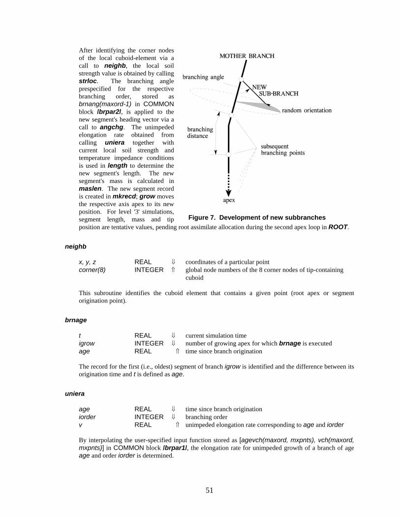
51

After identifying the corner nodes of the local cuboid-element via a call to neighb, the local soil strength value is obtained by calling strloc. The branching angle prespecified for the respective branching order, stored as brnang(maxord-1) in COMMON block /brpar2/, is applied to the new segment's heading vector via a call to angchg. The unimpeded elongation rate obtained from calling uniera together with current local soil strength and temperature impedance conditions is used in length to determine the new segment's length. The new segment's mass is calculated in maslen. The new segment record is created in mkrecd; grow moves the respective axis apex to its new position. For level '3' simulations, segment length, mass and tip position are tentative values, pending root assimilate allocation during the second apex loop in ROOT.

neighb

x, y, z corner(8)

REAL INTEGER

⇓ ⇑

coordinates of a particular point global node numbers of the 8 corner nodes of tip-containing cuboid

This subroutine identifies the cuboid element that contains a given point (root apex or segment origination point).

brnage

t igrow age

REAL INTEGER REAL

⇓ ⇓ ⇑

current simulation time number of growing apex for which brnage is executed time since branch origination

The record for the first (i.e., oldest) segment of branch igrow is identified and the difference between its origination time and t is defined as age.

uniera

age iorder v

REAL INTEGER REAL

⇓ ⇓ ⇑

time since branch origination branching order unimpeded elongation rate corresponding to age and iorder

By interpolating the user-specified input function stored as [agevch(maxord, mxpnts), vch(maxord, mxpnts)] in COMMON block /brpar1/, the elongation rate for unimpeded growth of a branch of age age and order iorder is determined.

Figure 7. Development of new subbranches

52

length

v dtroot newlen corner(8) temp toxi

REAL REAL REAL INTEGER LOGICAL LOGICAL

⇓ ⇓ ⇑ ⇓ ⇓ ⇓

unimpeded elongation rate corresponding to age and iorder finite growth time interval over which new segment developed length of new segment global node numbers of the 8 corner nodes of tip-containing cuboid set to .TRUE. if temperature data are provided set to .TRUE. if solute concentration effects on growth are included

A local impedance factor is calculated by taking the average of the impedance-due-to-soil-strength values, stored as imps(maxnod) in COMMON block /strgth/, at the eight corner nodes of the local cuboid-element. A similar average is obtained for the temperature impedance values that are stored as impt(maxnod) in COMMON block /tmptre/, if soil temperature values are provided, and for the solute concentration impedance values that are stored as impc(maxnod) in COMMON block /conimp/, if the effect of solute deficient or excessive concentration on root growth is being considered. Multiplying v, dtroot, and the three local impedance factor(s) gives the length of the new segment.

ssgcom

corner(8) stndrd strsen dxstr dystr dzstr

INTEGER REAL REAL REAL REAL REAL

⇓ ⇓ ⇓ ⇑ ⇑ ⇑

global node numbers of the 8 corner nodes of tip-containing cuboid common reference length for the different components making up the growth direction vector weighting factor for soil strength component of growth direction vector basic components of soil strength component of growth direction vector

The local soil strength gradient is approximated using the soil strength values, stored as s(maxnod) in COMMON block /strgth/, at the eight corner nodes of the local cuboid-element. The negative gradient is made unitless by dividing by the reference gradient value refgrd (in COMMON block /strpar/) and then multiplied with the reference length and the weighting factor to give dxstr, dystr, and dzstr.

geocom

tloc iord iax stndrd alpha dxgeo dygeo dzgeo

REAL INTEGER INTEGER REAL REAL REAL REAL REAL

⇓ ⇓ ⇓ ⇓ ⇓ ⇑ ⇑ ⇑

current local soil temperature branching order of the considered branch the number of the axis to whose branching system the considered branch belongs common reference length for the different components making up the growth direction vector heading angle azimuth basic components of geotropism component of growth direction vector

First, a preferential vertical growth angle and the weighting factor for the growth direction vector's geotropism angle component are determined via calling prfang. The basic components dxstr, dystr, and dzstr are obtained by multiplying the appropriate sine and cosine expressions of both the

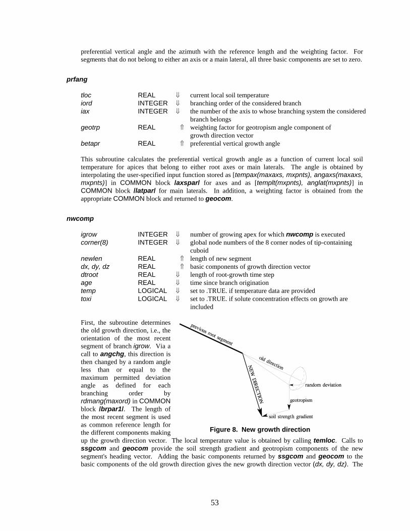
53

preferential vertical angle and the azimuth with the reference length and the weighting factor. For segments that do not belong to either an axis or a main lateral, all three basic components are set to zero.

prfang

tloc iord iax geotrp betapr

REAL INTEGER INTEGER REAL REAL

⇓ ⇓ ⇓ ⇑ ⇑

current local soil temperature branching order of the considered branch the number of the axis to whose branching system the considered branch belongs weighting factor for geotropism angle component of growth direction vector preferential vertical growth angle

This subroutine calculates the preferential vertical growth angle as a function of current local soil temperature for apices that belong to either root axes or main laterals. The angle is obtained by interpolating the user-specified input function stored as [tempax(maxaxs, mxpnts), angaxs(maxaxs, mxpnts)] in COMMON block /axspar/ for axes and as [templt(mxpnts), anglat(mxpnts)] in COMMON block /latpar/ for main laterals. In addition, a weighting factor is obtained from the appropriate COMMON block and returned to geocom.

nwcomp

igrow corner(8) newlen dx, dy, dz dtroot age temp toxi

INTEGER INTEGER REAL REAL REAL REAL LOGICAL LOGICAL

⇓ ⇓ ⇑ ⇑ ⇓ ⇓ ⇓ ⇓

number of growing apex for which nwcomp is executed global node numbers of the 8 corner nodes of tip-containing cuboid length of new segment basic components of growth direction vector length of root-growth time step time since branch origination set to .TRUE. if temperature data are provided set to .TRUE. if solute concentration effects on growth are included

First, the subroutine determines the old growth direction, i.e., the orientation of the most recent segment of branch igrow. Via a call to angchg, this direction is then changed by a random angle less than or equal to the maximum permitted deviation angle as defined for each branching order by rdmang(maxord) in COMMON block /brpar1/. The length of the most recent segment is used as common reference length for the different components making up the growth direction vector. The local temperature value is obtained by calling temloc. Calls to ssgcom and geocom provide the soil strength gradient and geotropism components of the new segment's heading vector. Adding the basic components returned by ssgcom and geocom to the basic components of the old growth direction gives the new growth direction vector (dx, dy, dz). The

Figure 8. New growth direction

54

unimpeded elongation rate obtained from calling uniera together with current local soil strength and temperature impedance conditions is used in length to determine the new segment's length.

angchg

dx, dy, dz alpha beta gamma delta

REAL REAL REAL REAL REAL

⇓ ⇑ ⇑ ⇑ ⇓ ⇓

vector components before and after the change of direction angle between the vector's horizontal projection and the x-axis (azimuth) vertical angle between the vector and its horizontal projection change to be applied to the vector's alpha change to be applied to the vector's beta

The angles defining the horizontal and vertical orientation of vector (dx, dy, dz), alpha and beta, are changed by angles gamma and delta, respectively. The length of the vector before and after the reorientation is identical.

maslen

sloc iorder mpl

REAL INTEGER REAL

⇓ ⇓ ⇑

current local soil strength branching order root-mass-per-length value corresponding to sloc and iorder

By interpolating the user-specified input function stored as [smplch(maxord, mxpnts), mplch(maxord, mxpnts)] in COMMON block /brpar3/, the mass-per-length value for a root segment in a soil neighborhood of soil strength sloc is determined.

mkrecd

igrow length mass t

INTEGER REAL REAL REAL

⇓ ⇓ ⇓ ⇓

number of growing apex creating the new segment length of new segment mass of new segment current simulation time

A new segment record is created in COMMON block /record/. First, the total number of segment records, nrec is incremented by one. The position of apex igrow at the beginning of the current root growth time step, [xg(igrow), yg(igrow), zg(igrow)] is then stored together with the current time, t as point and time of segment origination, [x(nrec), y(nrec), z(nrec)] and timorg(nrec), respectively. In addition, the values for branching order, global branching number, segment length and mass as well as the record number of the preceding segment are written into the record.

grow

igrow dx, dy, dz newlen

INTEGER REAL REAL

⇓ ⇓ ⇓

number of growing apex basic components of the growth direction vector growth increment of branch igrow during current time step

The length of the growth direction vector is scaled to match newlen before it is applied to advance the position of the apex igrow. The current position of each growing apex is stored as [xg(maxgrw), yg(maxgrw), zg(maxgrw)] in COMMON block /growth/. The most recently created segment is the segment immediately behind the apex. For later identification, its number (the current nrec) is stored as irecsg(igrow), also in /growth/.

55

adjust

igrow grwfac newlen

INTEGER REAL REAL

⇓ ⇓ ⇑

number of growing apex for which adjust is executed assimilate allocation factor for root growth growth increment of branch igrow during current time step

For level '3' simulations, the length and mass values of the new root segments created during the first apex loop in ROOT are tentative values in that they only represent the influence of the respective local soil environmental conditions. To have the new root growth match the available assimilates, an allocation factor grwfac is calculated in ROOT as the ratio between available assimilate, dmroot, and sumgrw, the cumulative need for root assimilate as determined during the first apex loop. An allocation factor greater than unity indicates more assimilate being sent to the root than the root can transform into new growth under the current conditions. In that case, the extra assimilate is assumed to be exuded. During the second apex loop in ROOT, adjust scales the length and mass of each new segment created during ROOT's first apex loop by the smaller of grwfac and 1.0. The limit of 1.0 represents the exudation assumption. The apex position [xg(igrow), yg(igrow), zg(igrow)] in COMMON block /growth/ is corrected accordingly. The total branch length, brlgth(igrow), also in /growth/, is updated in adjust for level '3' simulations, and in ROOT for lower-level simulations.

spacng

igrow space

INTEGER REAL

⇓ ⇑

number of growing apex for which spacng is executed distance between subbranches originating from branch igrow

The distance between subsequent subbranches is stored for each branching order as brspac(maxord-1) in COMMON block /brpar2/. The value corresponding to the branching order of branch igrow is returned as space. This module was created to permit easy implementation of future extensions that account for local environmental influences on the branching distance.

establ

igrow newlen space t dtroot

INTEGER REAL REAL REAL REAL

⇓ ⇓ ⇓ ⇓ ⇓

number of growing apex for which establ is executed length of root-growth time step distance between subbranches originating from branch igrow current simulation time length of root-growth time step

As part of ROOT's second apex loop, the list of established potential subbranch origination points for each apex igrow (COMMON block /estbsh/) is extended by the points that will be located on the most recent segment created by that apex during the current time step. To avoid storing of three space-coordinate values for each future branching point, the list contains the time at which each point has been established, assuming constant elongation rate during the root-growth time step. Using the same assumption, brdevl obtains the exact branching position from the stored time values for all subbranch origination points that develop into a new branch.

boxlim

igrow dtroot

INTEGER REAL

⇓ ⇓

number of growing apex length of root-growth time step

This subroutine is executed for each apex during ROOT's third apex loop. At that stage, the new position of each apex igrow is defined as [xg(igrow), yg(igrow), zg(igrow)] in COMMON block /growth/ while its previous position is stored as the segment origination point for the segment with

56

record number irecpr(igrow), the newly created segment immediately behind the apex igrow. Subroutine boxlim determines whether the new apex location is outside the domain limits as defined in COMMON block /domlim/. If that is the case, the side wall that is the first to be intersected by segment irecpr(igrow) is identified and the segment is broken apart at the wall. The part that was outside the domain becomes a new segment with orientation defined via a call to common. The position of apex igrow is corrected accordingly. The process is repeated if the new segment happens to extend across another side wall which is not unlikely if the old apex position was near one the domain's corners.

compon

wall irec dx, dy, dz

CHAR.*1 INTEGER REAL

⇓ ⇓ ⇓ ⇑

identifies either the x, y, or z-axis as being normal to the intersected side wall number of segment being broken apart vector components before and after the change of direction

The part of the segment that was outside the domain is reoriented along the projection of the old orientation onto the intersected side wall. If the intersection occurs within the immediate vicinity of a domain corner, the segment is orientated back into the domain.

remove

nrecol INTEGER ⇓ total number of segment records at the beginning of this execution of ROOT

Some of the root segments creating during this execution of ROOT may be insignificantly small, i.e., those in regions of very high soil strength. For memory efficiency and to prevent numerical problems, they are removed from the list of segment records in COMMON block /record/. The total number of segment records, nrec, is corrected accordingly.

update

ngrwnw INTEGER ⇓ total number of growing branches at the beginning of this execution of ROOT

This subroutine removes all branches that have reached their maximum length during this execution of ROOT from the list of growing branches in COMMON block /growth/ and updates the total number of growing branches, ngrow.

Output In addition to FEMs and root system output files, a log and a mass balance file are created during each simulation showing how important parameters change at each time step.

57

log

t tpot tact grwfac savg cavg mshoot mroot level

REAL REAL REAL REAL REAL REAL REAL REAL INTEGER

⇓ ⇓ ⇓ ⇓ ⇓ ⇓ ⇓ ⇓ ⇓

current simulation time potential transpiration at time t actual transpiration at time t assimilate allocation factor for root growth at time t average soil strength felt by root apices at time t average solute concentration felt by the root system at time t shoot mass at time t root mass at time t simulation level

At each FEM time step, one line is added to the log file. For each simulation level, the following parameters are written to the log file: level '1', t, savg, cavg, mroot; level '2', t, tpot, tact, savg, cavg, mroot; level '3', t, tpot, tact, grwfac, savg, cavg, mshoot, mroot.

outfem

t hnew(maxnod) conc(maxnod) matnum(maxnod) koufem

REAL REAL REAL INTEGER INTEGER

⇓ ⇓ ⇓ ⇓ ⇓

current simulation time nodal soil water pressure head values at the current time step nodal solute concentration values at the current time step nodal soil type numbers number of this FEM output file (counting variable)

For easy file identification, koufem is used as extension of the output file name. Each FEM output file contains in its first lines the user information stored in COMMON block /info/. In addition, an integration of the current volumetric water and solute content over the modeled soil domain is performed so that the total volume of water and solute present in the domain at time t can be written to the output file. The main part of the file consists of the list of current nodal.

outroo

t naxes mroot mshoot LA savg

REAL INTEGER REAL REAL REAL REAL

⇓ ⇓ ⇓ ⇓ ⇓ ⇓

current simulation time number of root axes present at time t root mass at time t shoot mass at time t leaf area at time t average soil strength felt by root apices at time t

A new output file is created with the current simulation time t being used as the file name. All available information describing the root system at time t is then written to this output file.

subreg

matnum(maxnod) conc(maxnod) t hnew(maxnod) lchem

INTEGER REAL REAL REAL LOGICAL

⇓ ⇓ ⇓ ⇓ ⇓

nodal soil type number nodal solute concentration values at the current time step current simulation time nodal water content values at the current time step set to .TRUE. if solute transport is being considered

This subroutine creates the file "balance.out" at the beginning of the simulation, recording the total initial volumetric water and solute content in the domain. A new line is then added to the file at each

58

time step, recording the current simulation time, the new water and solute contents, the absolute and relative errors in the water and solute mass balance and the Peclet and Courant numbers.

getout

Upon completing the last user-requested output file, a message is sent to the console and the simulation ends.

59

REFERENCES Barber, S. A., Soil Nutrient Bioavailability. A Mechanistic Approach, John Wiley &Sons,

New York, 1984. Bengough, A. G., and C. E. Mullins, Mechanical impedance to root growth, a review of

experimental techniques and root growth responses, J. Soil Sci., 41:341-358, 1990. Bengough, A. G., and C. E. Mullins, Penetrometer resistance, root penetration resistance

and root elongation rate in two sandy loam soils, Plant and Soil, 131:59-66, 1991. Bloom, A. J., L. E. Jackson, and D. R. Smart, Root growth as a function of ammonium and

nitrate in the root, Plant, Cell and Env., 16:199-206, 1993. Clausnitzer, V., and J. W. Hopmans, An algorithm for three-dimensional, simultaneous

modeling of root growth and transient soil water flow, V. 1.0, LAWR Paper no. 100022, Department of Land, Air and Water Resources, University of California, Davis, Ca., 1993.

Clausnitzer, V., and J. W. Hopmans, Simultaneous modeling of transient three-dimensional root growth and soil water flow, Plant and Soil, 164:299-314, 1994.

Diggle, A. J., ROOTMAP - a model in three-dimensional coordinates of the growth and structure of fibrous root systems, Plant and Soil, 105:169-178, 1988.

Ericsson, T., Growth and shoot: root ration of seedlings in relation to nutrient availability, Plant and Soil, 168-169:205-214, 1995.

Feddes, R. A., P. J. Kowalik, and H. Zaradny, Simulation of field water use and crop yield, Simulation Monographs, Pudoc, Wageningen, The Netherlands, 1978.

Fortin, M. A. and K. L. Poff, Temperature sensing by primary roots of maize, Plant Physiol., 94:367-369, 1990.

Gerard, C. J., The influence of soil moisture, soil texture, drying conditions, and exchangeable cations on soil strength, Soil Sci. Soc. Am. Proc., 29:641-645, 1965.

Goss, M. J., Effects of mechanical impedance on root growth in barley, J. Exp. Bot., 28:96-111, 1977.

Henriksen, G. H., D. R. Raman, L. P. Walker, and R. M. Spanswick, Measurement of net fluxes of ammonium and nitrate at the surface of barley roots using ion-selective microelectrodes: II. Patterns of uptake along the root axis and evaluation of the microelectrode flux estimation technique, Plant Physiol., 99:734-747, 1992.

Hillel, D., Introduction to Soil Physics, Academic Press, San Diego, Ca., 1980. Horwitz, B. A. and B. Zur, Gravitropic response of primary maize rootlets as influenced by

light and temperature, Plant, Cell and Env., 14:619-623, 1991. Jones, C. A., W. L. Bland, J. T. Ritchie, and J. R. Williams, Simulation of root growth, in:

Modeling Plant and Soil Systems, Agronomy Monograph no. 31, 1991. Kaspar, T. C. and W. L. Bland, Soil temperature and root growth, Soil Sci., 154:290-299,

1992. Kochian, L. V. and W. J. Lucas, Potassium transport in corn roots, Plant Physiol.,

70:1723-1731, 1982. Kutschera-Mitter, L., Über das geotrope Wachstum der Wurzel, Beitr. Biol. Pflanzen,

47:371-436, 1971. Kutschera-Mitter, L., Erklärung des geotropen Wachstums aus Standort und Bau der

Pflanzen, in: Land- und forstwirtschaftliche Forschung in Österreich, Österr. Agrarverlag Wien, 1972.

60

Kutschera-Mitter, L., Morphologie der Wurzeln von Arten des Acker- und Grünlandes und ihre Veränderung durch die Umwelt unter besonderer Berücksichtigung des geotropen Wachstums, in: R. Schubert, W. Hilbig, and E. Mahn (eds.), Probleme der Agrogeobotanik, Wiss. Beitr. der Martin-Luther-Univ. Halle, 1973.

Kutschera-Mitter, L., Positiver Geotropismus der Wurzel durch Asymmetrie der Haube, Beitr. Biol. Pflanzen, 52:57-81, 1976.

Lazof, D. B., T. W. Rufty, and M. G. Redinbaugh, Localization of nitrate absorption and translocation within morphological regions of the corn root, Plant Physiol., 100:1251-1258, 1992.

Lafolie, F., L. Bruckler, and F. Tardieu, Modeling root water potential and soil-root water transport: I. Model presentation, Soil Sci. Soc. Am. J., 55:1203-1212, 1991.

Masle, J., Genetic variation in the effects of root impedance on growth and transpiration rates of wheat and barley, Aust. J. Plant Physiol., 19:109-125, 1992.

Masle, J., G. D. Farquhar and R. M. Gifford, Growth and carbon economy of wheat seedlings as affected by soil resistance to penetration and ambient partial pressure of CO2, Aust. J. Plant Physiol., 17:465-487, 1990.

Masle, J., and J. B. Passioura, The effect of soil strength on the growth of young wheat plants, Aust. J. Plant Physiol., 14:643-656, 1987.

Molz, F. J., Models of water transport in the soil-plant system: a review, Water Resour. Res., 17:1245-1260, 1981.

Mosher, P. N. and M. H. Miller, Influence of soil temperature on the geotropic response of corn roots, Agron. J., 64:459-462, 1972.

Pages, L., M. O. Jordan, and D. Picard, A simulation model of the three-dimensional architecture of the maize root system, Plant and Soil, 119:147-154, 1989.

Schmidhalter, U., and J. J. Oertli, Transpiration/biomass ratio for carrots as affected by salinity, nutrient supply and soil aeration, Plant and Soil, 135:125-132, 1991.

Siddiqi, M. Y., A. D. M. Class, T. J. Ruth, T. W. Rufty, Studies of the uptake of nitrate in barley: 1. Kinetics of 13NO3

- influx, Plant Physiol., 93:1426-1432, 1990.

Silk, W. K., T. C. Hsiao, U. Diedenhofen, and C. Matson, Spatial distribution of potassium, solutes and their deposition rates in the growth zone of the primary corn root, Plant Physiol., 82:853-858, 1986.

Svimu°nek, J., T. Vogel, and M. Th. van Genuchten, The SWMS_2D code for simulating

water flow and solute transport in two-dimensional variably saturated media, V. 1.1, Research Report No. 126, U.S. Salinity Lab, ARS USDA, Riverside, Ca., 1992.

Smucker, A. J. M., Carbon utilization and losses by plant root systems, in: Roots, nutrient and water influx, and plant growth, ASA Special Publication no. 49, 1984.

Stark, N., The effects of water and multi-nutrient stress on xylem sap chemistry, photosynthesis and transpiration of seedlings of two Eucalypts, Trees, 6:7-12, 1992.

Taylor, H. M. and H. R. Gardner, Penetration of cotton seedling taproots as influenced by bulk density, moisture content, and strength of soil, Soil Sc., 96:153-156, 1963.

Taylor, H. M., G. M. Roberson, and J. J. Parker, Soil strength-root penetration relations for medium- to coarse-textured soil materials, Soil Sc., 102:18-22, 1966.

Taylor, H. M. and L. F. Ratliff, Root elongation rates of cotton and peanuts as a function of soil strength and soil water content, Soil Sc., 108:113-119, 1969.

61

Tucker, M. and C. von Seelhorst, Der Einfluß welchen der Wassergehalt und der Reichtum des Bodens auf die Ausbildung der Wurzeln und der oberirdischen Organe der Haferpflanze ausüben, J. Landwirtschaft, 46:52-63, 1898.

van Genuchten, M. Th., A closed-form equation for predicting the hydraulic conductivity of unsaturated soils, Soil Sci. Soc. Am. J., 44:892-898, 1980.

van Genuchten, M. Th., A numerical model for water and solute movement in and below the root zone, Research Report No. 121, U.S. Salinity Lab, ARS USDA, Riverside, Ca., 1987.

van Genuchten, M. Th. and S. K. Gupta, A reassessment of the crop tolerance response function, J. Indian Soc. Soil Sci., 4:730-737, 1993.

Vogel, T., SWM II - numerical model of two-dimensional flow in a variably saturated porous medium, Research Report No. 87, Wageningen Agricultural Univ., The Netherlands, 1987.

Voorhees, W. B., D. A. Farrell and W. E. Larson, Soil strength and aeration effects on root elongation, Soil Sci. Soc. Am. Proc., 39:948-953, 1975.

62

APPENDIX A: Numerical solution of water flow and solute transport equations In the next pages the main steps will be presented, involved in the numerical solution of the three-dimensional versions of equations (1) and (2). The main outline follows the two-dimensional development of the equations by S

vimu°nek et al., (1992), to which the reader is referred for further

details, underlying assumptions and additional references.

Water flow equation - The governing equation (1) is reported here:

∂θ∂

∂∂

∂∂t x

Khx

Si

ijA

jizA= + −[ (K K )] . (A.1)

The simulation domain has been discretized in a grid of tetrahedral elements. The standard Galerkin's finite element method has been used, requiring that the differential operator associated with (A.1) be orthogonal to each of the N basis function, N being the total number of nodes in the discretized domain W:

[ (K K )] d 0∂θ∂

∂∂

∂∂

ϕt x

Khx

S Wi

ijA

jizA

Wn− + + =∫ . (A.2)

Substituting h(x,y,z,t) with h':

h x y z t x y z h tnn

N

n' , , , , ,( ) ( ) ( )==

∑ϕ1

; (A.3)

where ϕn are the linear basis functions and hn are the weighting coefficients representing the solution of (A.1), and applying Green's theorem to the resulting expression we obtain:

( K )d

(K K ) d ( K )d

∂θ∂

ϕ∂∂

∂ϕ∂

∂∂

ϕ∂ϕ∂

ϕ

tK

hx x

W

Khx

n Kx

S W

n ijA

jWe

n

i

ijA

jeizA

i n izA

We

n

in

e

e e

+ =

+ + − −

∫∑

∫∑ ∫∑

'

';

Ω

Ω (A.4)

where We is the volume of element e and Ωe its the boundary area.

The system of equations can be rearranged in the following matrix form:

[ ]d d

[ ] Ft

A h Q B Dθ

+ = − − ; (A.5)

where:

A Kx x

W

KV

b b c c d d b c c b

b d d b c d d c

mn l ijA

el

m

i

n

jW

eem n xx

Am n yy

An zz

Am n m n xy

A

m n m n xzA

m n m n yzA

e

= =

= + + + + +

+ + + +

∑ ∫

∑

K d

[ K K K ( )K

( )K ( )K

m

ϕ ∂ϕ∂

∂ϕ∂

36

;

(A.6)

63

( )B Kx

WK

b c dn l izA

el

n

iW exzA

n yzA

n zzA

ne

= = + +∑ ∫ ∑K d K K Kϕ∂ϕ∂ 6

; (A.7)

F WV

mn mn nWe

mne

ee

= =∫∑ ∑δ ϕ δd4

; (A.8)

( )QA

n le

l nn

nee

= − = − +∑ ∫ ∑σ ϕ ϕ σ σdΩΩ 12

4 ; (A.9)

( )D S WV

S Sn le

l nW

en

ee

= = +∑ ∫ ∑ϕ ϕ d20

4 ; (A.10)

where V and A are the volume and the boundary area of element e. The overlined variables represent the average values over element; subscripts i and j refer to the spatial coordinates (i,j = 1,2,3) and l, m, n vary between 1 and N.

Equation (A.5) is integrated in time using a backward finite difference scheme, resulting in the following system of equations:

[ ]

[ ] Ft

A h Q B Dj j

jj j j j j

θ θ++ + + + +

−+ = − −1

1 1 1 1 1∆; (A.11)

with j+1 and j being the current and previous time levels, respectively, and ∆tj = tj+1 – tj.

Solute transport equation - Equation (2) is reported here in the following form:

− − + + + =θ∂∂

∂∂

∂∂

θ∂∂

Rct

qcx x

cx

Fc Gii i

ijj

( D ) 0 ; (A.12)

where:

F k S SG

w s

w s

= + + −= +

µ θ µ ργ θ γ ρ

' ;;

(A.13)

and:

Rk

= +1ρθ

. (A.14)

Following the same reasoning presented above we obtain:

[ ( D ) ] d− − + + + =∫ θ∂∂

∂∂

∂∂

θ∂∂

ϕRct

qcx x

cx

Fc G WW

ii i

ijj

n 0 . (A.15)

Substituting c(x,y,z,t) with c':

c x y z t x y z c tn

N

n' , , , , ,( ) ( ) ( )= ∑ϕ1

; (A.16)

where, again, ϕn are the linear basis functions and cn are the weighting coefficient representing the solution of (A.12), and applying Green's theorem to the resulting expression we obtain:

64

[( ) D ]d

D d

− − + + − +

+ =

∫∑

∫∑

θ∂∂

∂∂

ϕ θ∂∂

∂ϕ∂

θ∂∂

ϕ

Rct

qcx

Fc Gcx x

W

cx

n

ii

n ijj

n

iWe

ijj

i ne

e

Ne

' ''

'

';

Ω

Ω 0 (A.17)

where We is the volume of element e and Ωe the boundary area of the e.

The system of equations is then rearranged in the following matrix form:

[ ]d d

[ ] Qct

S c f QD+ + = − ; (A.18)

where:

S qx

Wx x

W

F W

bq q

cq q

dq q

VF F F

Vb b c c d d

nm i l l nm

iij l

Wl

n

i

m

jWe

l l n mW

mx xn

my yn

mz zn

e

en m nm

en m xx n m yy n

e e

e

= − − +

+ =

= − + − + − + +

+ + + + +

− + +

∫ ∫∑

∫

∑

[( ) d ( D ) d

d

( ) ( ) ( )

( )( )

[ D D

ϕ ϕ∂ϕ∂

θ ϕ∂ϕ∂

∂ϕ∂

ϕ ϕ ϕ

δ

θ θ

]

1204

1204

1204

1204 1

136 m zz n m n m xy

n m n m xz n m n m yz

b c c b

b d d b c d d c

θ θ

θ θ

D ( ) D

( ) D ( ) D ]

+ + +

+ + + + ;

(A.19)

and:

Q R WV

R Rnm l l n mWe

en nm

ee

= − = − +∫∑ ∑( ) d ( )θ ϕ ϕ ϕ θ θ δ20

4 ; (A.20)

f G WV

G Gn l l nWe

en

ee

= = +∫∑ ∑ϕ ϕ d ( )20

4 ; (A.21)

Equation (A.18) is integrated in time using a finite difference scheme, resulting in the following system of equations:

[ ]

[ ] ( )[ ]

( )

Qc c

tS c S c

f f

jj j

jj j j j

j j

++

+ + +

+

−+ − +

+ + − =

ε ε ε

ε ε

11 1

1

1

1 0∆

; (A.22)

with j+1 and j being the current and previous time levels, respectively, and ε the time weighing coefficient.

65

APPENDIX B: Variables in COMMON blocks COMMON /approx/

shared by: chemin, SOLUTE, c_bound, chinit

epsi nlevel

REAL INTEGER

temporal weighing coefficient for the solute transport FEM scheme number of steps required in assembling the matrix A and the vector B for the solute FEM scheme

COMMON /axes/

shared by: MAIN, rootin, ROOT, newaxs

naxemg tnewax(maxemg) nnewax(maxemg)

INTEGER REAL INTEGER

number of axis group emergence events time of each emergence event number of emerging axes for each emergence event

COMMON /axspar/

shared by: rootin, prfang

nangax(maxaxs) tempax(maxaxs, mxpnts) angaxs(maxaxs, mxpnts) geoaxs(maxaxs)

INTEGER REAL REAL REAL

number of (temperature, angle)-points making up stepwise linear input function for geotropism angle of each axis temperature values of stepwise linear input function for each axispreferred-angle values of stepwise linear input function for each axis weighting factor for geotropism angle component of growth direction vector for each axis

COMMON /bndary/

shared by: applic, setbc, c_bound

ibcpt(maxbdr) nqbcch tqbcch(mxbcch) qbc(mxbcch) nhbcch thbcch(mxbcch) hbc(mxbcch) ncbnd1 tcbnd1(mxbcch) cbnd1(mxbcch) ncbnd2 tcbnd2(mxbcch) cbnd2(mxbcch)

INTEGER INTEGER REAL REAL INTEGER REAL REAL INTEGER REAL REAL INTEGER REAL REAL

global node numbers of nodes for which boundary conditions have been specified number of (time, water flux)-points making up stepwise linear flux-B.C. function time values of stepwise linear flux-B.C. function water flux values of stepwise linear flux-B.C. function number of (time, head)-points making up stepwise linear head-B.C. function time-values of stepwise linear head-B.C. function head-values of stepwise linear head-B.C. function number of (time, B.C. value)-points making up stepwise linear B.C. function time values of stepwise linear B.C. function B.C. values of stepwise linear B.C. function number of (time, B.C. value)-points making up stepwise linear B.C. function time values of stepwise linear B.C. function B.C. values of stepwise linear B.C. function

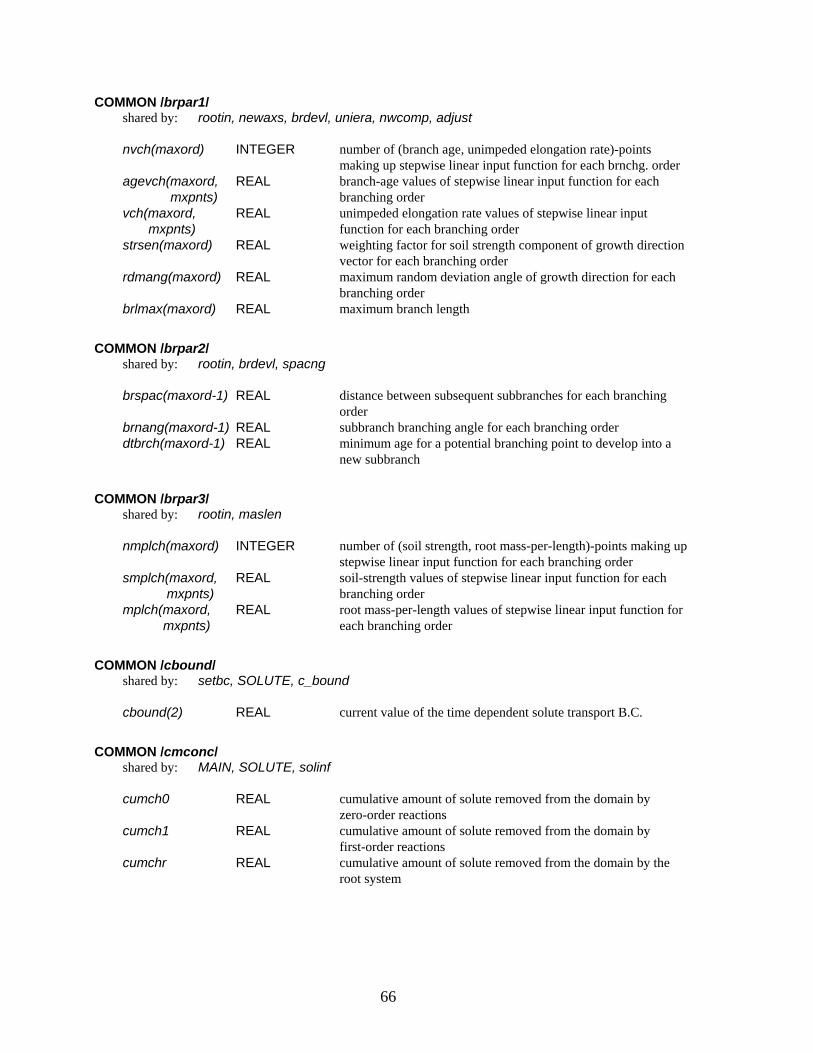
66

COMMON /brpar1/ shared by: rootin, newaxs, brdevl, uniera, nwcomp, adjust

nvch(maxord) agevch(maxord, mxpnts) vch(maxord, mxpnts) strsen(maxord) rdmang(maxord) brlmax(maxord)

INTEGER REAL REAL REAL REAL REAL

number of (branch age, unimpeded elongation rate)-points making up stepwise linear input function for each brnchg. order branch-age values of stepwise linear input function for each branching order unimpeded elongation rate values of stepwise linear input function for each branching order weighting factor for soil strength component of growth direction vector for each branching order maximum random deviation angle of growth direction for each branching order maximum branch length

COMMON /brpar2/

shared by: rootin, brdevl, spacng

brspac(maxord-1) brnang(maxord-1) dtbrch(maxord-1)

REAL REAL REAL

distance between subsequent subbranches for each branching order subbranch branching angle for each branching order minimum age for a potential branching point to develop into a new subbranch

COMMON /brpar3/

shared by: rootin, maslen

nmplch(maxord) smplch(maxord, mxpnts) mplch(maxord, mxpnts)

INTEGER REAL REAL

number of (soil strength, root mass-per-length)-points making up stepwise linear input function for each branching order soil-strength values of stepwise linear input function for each branching order root mass-per-length values of stepwise linear input function for each branching order

COMMON /cbound/

shared by: setbc, SOLUTE, c_bound

cbound(2) REAL current value of the time dependent solute transport B.C.

COMMON /cmconc/

shared by: MAIN, SOLUTE, solinf

cumch0 cumch1 cumchr

REAL REAL REAL

cumulative amount of solute removed from the domain by zero-order reactions cumulative amount of solute removed from the domain by first-order reactions cumulative amount of solute removed from the domain by the root system

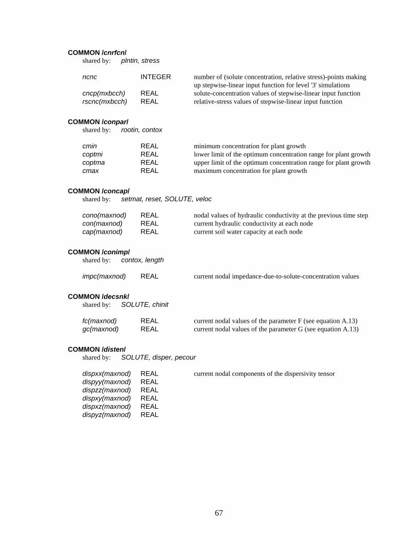
67

COMMON /cnrfcn/ shared by: plntin, stress

ncnc cncp(mxbcch) rscnc(mxbcch)

INTEGER REAL REAL

number of (solute concentration, relative stress)-points making up stepwise-linear input function for level '3' simulations solute-concentration values of stepwise-linear input function relative-stress values of stepwise-linear input function

COMMON /conpar/

shared by: rootin, contox

cmin coptmi coptma cmax

REAL REAL REAL REAL

minimum concentration for plant growth lower limit of the optimum concentration range for plant growthupper limit of the optimum concentration range for plant growthmaximum concentration for plant growth

COMMON /concap/

shared by: setmat, reset, SOLUTE, veloc

cono(maxnod) con(maxnod) cap(maxnod)

REAL REAL REAL

nodal values of hydraulic conductivity at the previous time step current hydraulic conductivity at each node current soil water capacity at each node

COMMON /conimp/

shared by: contox, length

impc(maxnod) REAL current nodal impedance-due-to-solute-concentration values

COMMON /decsnk/

shared by: SOLUTE, chinit

fc(maxnod) gc(maxnod)

REAL REAL

current nodal values of the parameter F (see equation A.13) current nodal values of the parameter G (see equation A.13)

COMMON /disten/

shared by: SOLUTE, disper, pecour

dispxx(maxnod) dispyy(maxnod) dispzz(maxnod) dispxy(maxnod) dispxz(maxnod) dispyz(maxnod)

REAL REAL REAL REAL REAL REAL

current nodal components of the dispersivity tensor

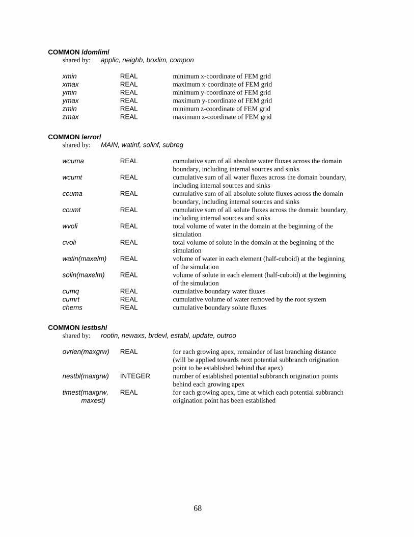
68

COMMON /domlim/ shared by: applic, neighb, boxlim, compon

xmin xmax ymin ymax zmin zmax

REAL REAL REAL REAL REAL REAL

minimum x-coordinate of FEM grid maximum x-coordinate of FEM grid minimum y-coordinate of FEM grid maximum y-coordinate of FEM grid minimum z-coordinate of FEM grid maximum z-coordinate of FEM grid

COMMON /error/

shared by: MAIN, watinf, solinf, subreg

wcuma wcumt ccuma ccumt wvoli cvoli watin(maxelm) solin(maxelm) cumq cumrt chems

REAL REAL REAL REAL REAL REAL REAL REAL REAL REAL REAL

cumulative sum of all absolute water fluxes across the domain boundary, including internal sources and sinks cumulative sum of all water fluxes across the domain boundary, including internal sources and sinks cumulative sum of all absolute solute fluxes across the domain boundary, including internal sources and sinks cumulative sum of all solute fluxes across the domain boundary, including internal sources and sinks total volume of water in the domain at the beginning of the simulation total volume of solute in the domain at the beginning of the simulation volume of water in each element (half-cuboid) at the beginning of the simulation volume of solute in each element (half-cuboid) at the beginning of the simulation cumulative boundary water fluxes cumulative volume of water removed by the root system cumulative boundary solute fluxes

COMMON /estbsh/

shared by: rootin, newaxs, brdevl, establ, update, outroo

ovrlen(maxgrw) nestbl(maxgrw) timest(maxgrw, maxest)

REAL INTEGER REAL

for each growing apex, remainder of last branching distance (will be applied towards next potential subbranch origination point to be established behind that apex) number of established potential subbranch origination points behind each growing apex for each growing apex, time at which each potential subbranch origination point has been established

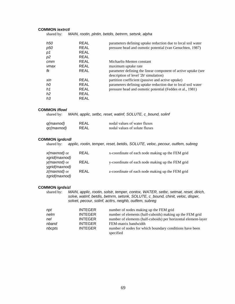
69

COMMON /extrct/ shared by: MAIN, rootin, plntin, betdis, betnrm, setsnk, alpha

h50 p50 p1 p2 cmm vmax fk xin h0 h1 h2 h3

REAL REAL REAL REAL REAL REAL REAL REAL REAL REAL REAL REAL

parameters defining uptake reduction due to local soil water pressure head and osmotic potential (van Genuchten, 1987) Michaelis-Menten constant maximum uptake rate parameter defining the linear component of active uptake (see description of level '2b' simulation) partition coefficient (passive and active uptake) parameters defining uptake reduction due to local soil water pressure head and osmotic potential (Feddes et al., 1981)

COMMON /flow/

shared by: MAIN, applic, setbc, reset, watinf, SOLUTE, c_bound, solinf

q(maxnod) qc(maxnod)

REAL REAL

nodal values of water fluxes nodal values of solute fluxes

COMMON /grdcrd/

shared by: applic, rootin, temper, reset, betdis, SOLUTE, veloc, pecour, outfem, subreg

x(maxnod) or xgrid(maxnod)

REAL x-coordinate of each node making up the FEM grid

y(maxnod) or ygrid(maxnod)

REAL y-coordinate of each node making up the FEM grid

z(maxnod) or zgrid(maxnod)

REAL z-coordinate of each node making up the FEM grid

COMMON /grdsiz/

shared by: MAIN, applic, rootin, solstr, temper, contox, WATER, setbc, setmat, reset, dirich, solve, watinf, betdis, betnrm, setsnk, SOLUTE, c_bound, chinit, veloc, disper, solvet, pecour, solinf, acttrs, neighb, outfem, subreg

npt nelm nel nband nbcpts

INTEGER INTEGER INTEGER INTEGER INTEGER

number of nodes making up the FEM grid number of elements (half-cuboids) making up the FEM grid number of elements (half-cuboids) per horizontal element-layer FEM-matrix bandwidth number of nodes for which boundary conditions have been specified

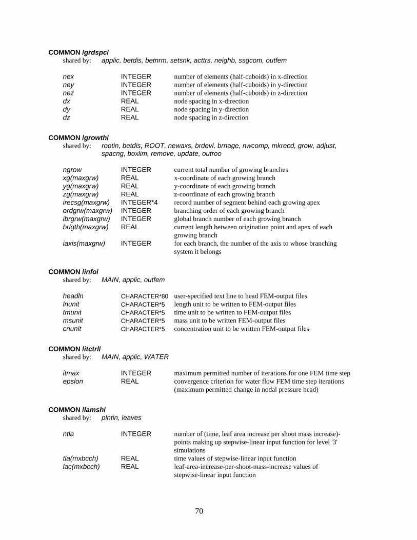
70

COMMON /grdspc/ shared by: applic, betdis, betnrm, setsnk, acttrs, neighb, ssgcom, outfem

nex ney nez dx dy dz

INTEGER INTEGER INTEGER REAL REAL REAL

number of elements (half-cuboids) in x-direction number of elements (half-cuboids) in y-direction number of elements (half-cuboids) in z-direction node spacing in x-direction node spacing in y-direction node spacing in z-direction

COMMON /growth/

shared by: rootin, betdis, ROOT, newaxs, brdevl, brnage, nwcomp, mkrecd, grow, adjust, spacng, boxlim, remove, update, outroo

ngrow xg(maxgrw) yg(maxgrw) zg(maxgrw) irecsg(maxgrw) ordgrw(maxgrw) ibrgrw(maxgrw) brlgth(maxgrw) iaxis(maxgrw)

INTEGER REAL REAL REAL INTEGER*4 INTEGER INTEGER REAL INTEGER

current total number of growing branches x-coordinate of each growing branch y-coordinate of each growing branch z-coordinate of each growing branch record number of segment behind each growing apex branching order of each growing branch global branch number of each growing branch current length between origination point and apex of each growing branch for each branch, the number of the axis to whose branching system it belongs

COMMON /info/

shared by: MAIN, applic, outfem

headln lnunit tmunit msunit cnunit

CHARACTER*80 CHARACTER*5 CHARACTER*5 CHARACTER*5 CHARACTER*5

user-specified text line to head FEM-output files length unit to be written to FEM-output files time unit to be written to FEM-output files mass unit to be written FEM-output files concentration unit to be written FEM-output files

COMMON /itctrl/

shared by: MAIN, applic, WATER

itmax epslon

INTEGER REAL

maximum permitted number of iterations for one FEM time stepconvergence criterion for water flow FEM time step iterations (maximum permitted change in nodal pressure head)

COMMON /lamsh/

shared by: plntin, leaves

ntla tla(mxbcch) lac(mxbcch)

INTEGER REAL REAL

number of (time, leaf area increase per shoot mass increase)-points making up stepwise-linear input function for level '3' simulations time values of stepwise-linear input function leaf-area-increase-per-shoot-mass-increase values of stepwise-linear input function

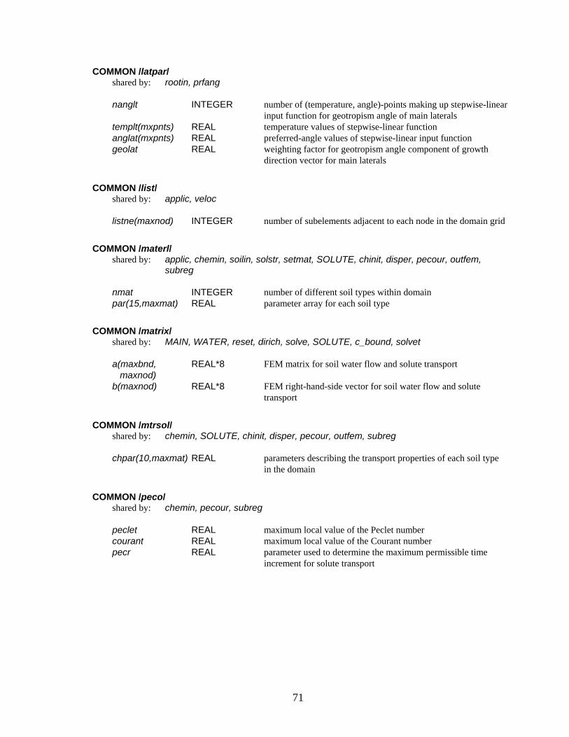
71

COMMON /latpar/ shared by: rootin, prfang

nanglt templt(mxpnts) anglat(mxpnts) geolat

INTEGER REAL REAL REAL

number of (temperature, angle)-points making up stepwise-linear input function for geotropism angle of main laterals temperature values of stepwise-linear function preferred-angle values of stepwise-linear input function weighting factor for geotropism angle component of growth direction vector for main laterals

COMMON /list/

shared by: applic, veloc

listne(maxnod) INTEGER number of subelements adjacent to each node in the domain grid

COMMON /materl/

shared by: applic, chemin, soilin, solstr, setmat, SOLUTE, chinit, disper, pecour, outfem, subreg

nmat par(15,maxmat)

INTEGER REAL

number of different soil types within domain parameter array for each soil type

COMMON /matrix/

shared by: MAIN, WATER, reset, dirich, solve, SOLUTE, c_bound, solvet

a(maxbnd, maxnod) b(maxnod)

REAL*8 REAL*8

FEM matrix for soil water flow and solute transport FEM right-hand-side vector for soil water flow and solute transport

COMMON /mtrsol/

shared by: chemin, SOLUTE, chinit, disper, pecour, outfem, subreg

chpar(10,maxmat) REAL parameters describing the transport properties of each soil type in the domain

COMMON /peco/

shared by: chemin, pecour, subreg

peclet courant pecr

REAL REAL REAL

maximum local value of the Peclet number maximum local value of the Courant number parameter used to determine the maximum permissible time increment for solute transport

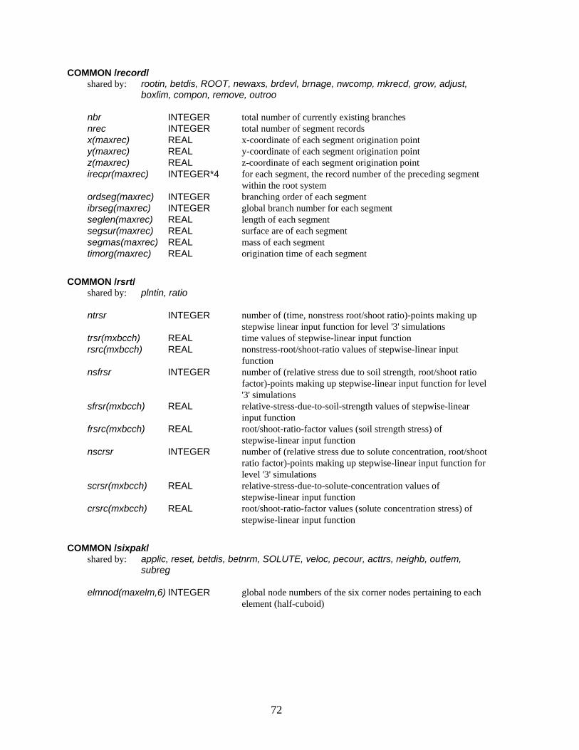
72

COMMON /record/ shared by: rootin, betdis, ROOT, newaxs, brdevl, brnage, nwcomp, mkrecd, grow, adjust,

boxlim, compon, remove, outroo

nbr nrec x(maxrec) y(maxrec) z(maxrec) irecpr(maxrec) ordseg(maxrec) ibrseg(maxrec) seglen(maxrec) segsur(maxrec) segmas(maxrec) timorg(maxrec)

INTEGER INTEGER REAL REAL REAL INTEGER*4 INTEGER INTEGER REAL REAL REAL REAL

total number of currently existing branches total number of segment records x-coordinate of each segment origination point y-coordinate of each segment origination point z-coordinate of each segment origination point for each segment, the record number of the preceding segment within the root system branching order of each segment global branch number for each segment length of each segment surface are of each segment mass of each segment origination time of each segment

COMMON /rsrt/

shared by: plntin, ratio

ntrsr trsr(mxbcch) rsrc(mxbcch) nsfrsr sfrsr(mxbcch) frsrc(mxbcch) nscrsr scrsr(mxbcch) crsrc(mxbcch)

INTEGER REAL REAL INTEGER REAL REAL INTEGER REAL REAL

number of (time, nonstress root/shoot ratio)-points making up stepwise linear input function for level '3' simulations time values of stepwise-linear input function nonstress-root/shoot-ratio values of stepwise-linear input function number of (relative stress due to soil strength, root/shoot ratio factor)-points making up stepwise-linear input function for level '3' simulations relative-stress-due-to-soil-strength values of stepwise-linear input function root/shoot-ratio-factor values (soil strength stress) of stepwise-linear input function number of (relative stress due to solute concentration, root/shoot ratio factor)-points making up stepwise-linear input function for level '3' simulations relative-stress-due-to-solute-concentration values of stepwise-linear input function root/shoot-ratio-factor values (solute concentration stress) of stepwise-linear input function

COMMON /sixpak/

shared by: applic, reset, betdis, betnrm, SOLUTE, veloc, pecour, acttrs, neighb, outfem, subreg

elmnod(maxelm,6) INTEGER global node numbers of the six corner nodes pertaining to each

element (half-cuboid)

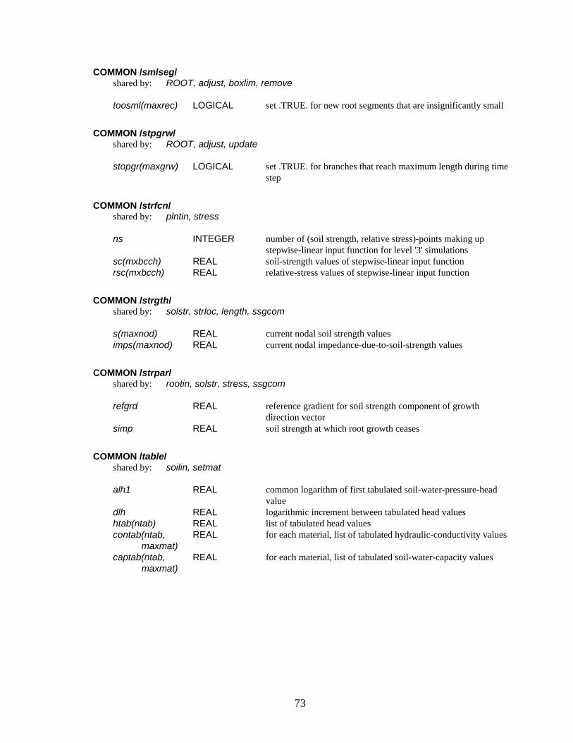
73

COMMON /smlseg/ shared by: ROOT, adjust, boxlim, remove

toosml(maxrec) LOGICAL set .TRUE. for new root segments that are insignificantly small

COMMON /stpgrw/

shared by: ROOT, adjust, update

stopgr(maxgrw) LOGICAL set .TRUE. for branches that reach maximum length during time step

COMMON /strfcn/

shared by: plntin, stress

ns sc(mxbcch) rsc(mxbcch)

INTEGER REAL REAL

number of (soil strength, relative stress)-points making up stepwise-linear input function for level '3' simulations soil-strength values of stepwise-linear input function relative-stress values of stepwise-linear input function

COMMON /strgth/

shared by: solstr, strloc, length, ssgcom

s(maxnod) imps(maxnod)

REAL REAL

current nodal soil strength values current nodal impedance-due-to-soil-strength values

COMMON /strpar/

shared by: rootin, solstr, stress, ssgcom

refgrd simp

REAL REAL

reference gradient for soil strength component of growth direction vector soil strength at which root growth ceases

COMMON /table/

shared by: soilin, setmat

alh1 dlh htab(ntab) contab(ntab, maxmat) captab(ntab, maxmat)

REAL REAL REAL REAL REAL

common logarithm of first tabulated soil-water-pressure-head value logarithmic increment between tabulated head values list of tabulated head values for each material, list of tabulated hydraulic-conductivity values for each material, list of tabulated soil-water-capacity values

74

COMMON /tempar/ shared by: rootin, temper, temloc

tmin topt tmax trange tmid expo

REAL REAL REAL REAL REAL REAL

minimum temperature for plant growth optimum temperature for plant growth maximum temperature for plant growth tmax - tmin (tmin + tmax)/2 exponent for root elongation rate vs. local temperature function

COMMON /temptm/

shared by: tempin, temper

nt nz time(mxtime) depth(mxdpth) temtim(mxtime, mxdpth)

INTEGER INTEGER REAL REAL REAL

Parameters describing stepwise-linear soil temperature = f(time,depth) input function: number of time values number of depth values time values depth values temperature values for each depth/time

COMMON /tensor/

shared by: applic, reset, SOLUTE, veloc

conaxx(maxelm) conayy(maxelm) conazz(maxelm) conaxy(maxelm) conaxz(maxelm) conayz(maxelm)

REAL REAL REAL REAL REAL REAL

unitless components of the conductivity tensor for each element (half-cuboid)

COMMON /tmctrl/

shared by: MAIN, applic, WATER, tmcon, ROOT

tmax dtmin dtmax facinc facdec dtroot noufem toufem(mxofem) nouroo touroo(mxoroo)

REAL REAL REAL REAL REAL REAL INTEGER REAL INTEGER REAL

time at which simulation ends (i.e., the latest user-specified output time) smallest permitted time step length greatest permitted time step length factor for time step length increase if convergence quick factor for time step length decrease if convergence slow time between subsequent root growth events number of desired FEM output files during simulation times at which FEM output is desired number of desired root output files during simulation times at which root output is desired

COMMON /tmptre/

shared by: temper, temloc, setsnk, length

tem(maxnod) impt(maxnod)

REAL REAL

current nodal soil-temperature values current nodal impedance-due-to-soil-temperature values

75

COMMON /tplat/ shared by: plntin, settp

nttpla ttpla(mxbcch) tplac(mxbcch) nftpla sftpla(mxbcch) ftplac(mxbcch) nctpla sctpla(mxbcch) ctplac(mxbcch)

INTEGER REAL REAL INTEGER REAL REAL INTEGER REAL REAL

number of (time, nonstress potential transpiration per leaf area)-points making up stepwise-linear input function for level '3' simulations time values of stepwise-linear input function nonstress-potential-transpiration-per-leaf-area values of stepwise-linear input function number of (relative stress due to soil strength, transpiration factor)-points making up stepwise-linear input function for level '3' simulations relative-stress-due-to-soil-strength values of stepwise-linear input function transpiration-factor values (soil strength stress) of stepwise-linear input function number of (relative stress due to solute concentration, transpiration factor)-points making up stepwise-linear input function for level '3' simulations relative-stress-due-to-solute-concentration values of stepwise-linear input function transpiration-factor values (solute concentration stress) of stepwise-linear input function

COMMON /tptime/

shared by: plntin, settp

ntpot ttpot(mxbcch) tpotc(mxbcch)

INTEGER REAL REAL

number of (time, potential transpiration)-points making up stepwise-linear Tpot-B.C. function for level '2' simulations time values of stepwise-linear Tpot-B.C. function potential-transpiration values of stepwise-linear Tpot-B.C. function

COMMON /upredf/

shared by: rootin, betdis

nurf age urf

INTEGER REAL REAL

number of (segment age, reduction factor)-points making up the stepwise-linear input function for level '2' and '3' simulations segment-age values of the stepwise-linear input function reduction factor values of the stepwise-linear input function

COMMON /uptake/

shared by: reset, watinf, betdis, betnrm, setsnk, SOLUTE, chinit, acttrs, outfem

betaw(maxnod) betac(macnod) sink(maxnod) csink(maxnod) rootsk(maxnod)

REAL REAL REAL REAL REAL

current nodal values of root distribution function (water uptake) current nodal values of root surface distribution function (solute uptake) current nodal values of the water flow sink term current nodal values of solute transport sink term current volume of water removed by the root system per unit time

76

COMMON /veloct/ shared by: SOLUTE, veloc, disper, pecour

vx(maxnod) vy(maxnod) vz(maxnod)

REAL REAL REAL

nodal values of volumetric flux components

COMMON /wt/

shared by: plntin, effncy

ntw tw(mxbcch) wc(mxbcch) nsfw sfw(mxbcch) fwc(mxbcch) nscw scw(mxbcch) cwc(mxbcch)

INTEGER REAL REAL INTEGER REAL REAL INTEGER REAL REAL

number of (time, nonstress water use efficiency)-points making up stepwise-linear input function for level '3' simulations time values of stepwise-linear input function nonstress-water-use-efficiency values of stepwise-linear input function number of (relative stress due to soil strength, water use efficiency factor)-points making up stepwise-linear input function for level '3' simulations relative-stress-due-to-soil-strength values of stepwise-linear input function water-use-efficiency-factor values (soil strength stress) of stepwise-linear input function number of (relative stress due to solute concentration, water use efficiency factor)-points making up stepwise-linear input function for level '3' simulations relative-stress-due-to-solute-concentration values of stepwise-linear input function water-use-efficiency-factor values (solute concentration stress) of stepwise-linear input function