AC 2009-575: AN ALTERNATIVE APPROACH FOR TEACHING MULTIBODYDYNAMICS

George Sutherland, Rochester Institute of TechnologyDR. GEORGE H. SUTHERLAND is a professor in the Manufacturing & MechanicalEngineering Technology and Packaging Science Department at the Rochester Institute ofTechnology in New York State. Dr. Sutherland’s technical interests include the dynamics of highspeed machinery and vehicle dynamics. He was previously an associate professor in ME at OhioState University, a manager at General Electric, a VP at CAMP Inc and President of WashingtonManufacturing Services.

© American Society for Engineering Education, 2009

Page 14.174.1

Page 14.174.2

Implicit Constraint Approach

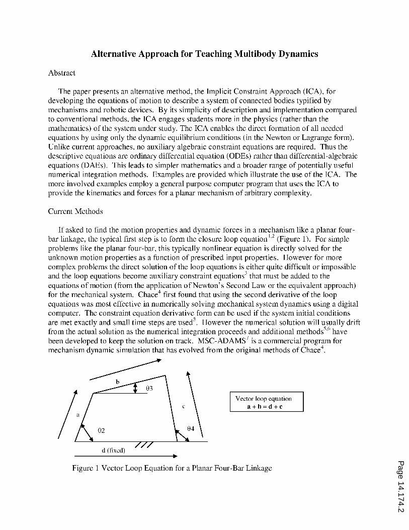
The underlying assumption in current mechanism analysis approaches is that the joints, which

connect the moving rigid bodies, are ideal in their behavior. The concept of forming a

mechanism model using a standard set of idealized joints dates back to Reuleaux8, and is still the

underlying assumption in modern dynamic analysis computer programs like MSC-Adams,

MathWorks SimMechanics9, and Working Model

10. When joints, like roller bearings, are rigidly

mounted and preloaded, radial stiffnesses of 108 N/m and higher

11 are typical and the ideal joint

assumption is reasonable. However when joints are designed with clearances and flexible

mounts, the ideal joint assumption might not be acceptable (depending on the analyst’s need).

The Implicit Constraint Approach (ICA)12

offers an alternative approach to mechanism

analysis where joint flexibility is an inherent characteristic utilized in the method. The relative

kinematic characteristics of standard joints are not used as basic assumptions. Instead each joint

type is characterized by the forces that are generated when the two components of the joint are

displaced relative to each other. A revolute joint (in three dimensions) is characterized by three

orthogonal reaction force components and two orthogonal reaction moment components. There

is no reaction moment about the axis that corresponds to the direction of joint relative rotation.

(In a two dimensional analysis this simplifies to just two orthogonal reaction forces acting in the

plane through the revolute joint center, while the moment reaction about the axis perpendicular

to the plane of motion is zero.) Using the ICA, these unknown reaction forces are assumed to be

proportional to the joint component relative displacements. Although there is a more rigorous

axiomatic underpinning to the ICA12

, it can be visualized by considering the joint components to

be connected to each other by specially-defined zero free length springs as shown for a planar

four-bar linkage in Figure 2.

Figure 2 Revolute Joints Represented by Zero Free Length Springs

Each joint type has a uniquely defined characteristic point12

in each connected body that

provides a reference point for calculating the joint reaction forces in terms of the joint

component relative displacements. Thus each joint is represented by two characteristic points

(one in each connected body) and the manner in which these two points are separated for a

specific joint type determines the joint reaction forces. For revolute (turning) joints the

characteristic points are the joint centers in each connected body. For prismatic (sliding) joints

k1

k2

k3

k4

Page 14.174.3

the characteristic point in each body is the point on the sliding axis where an orthogonal line

from the body’s mass center intersects the axis. For a planar prismatic joint there is a reaction

moment proportional to the relative rotation of the two joint component sliding axes and a

normal force proportional to the separation of the two axes as measured at one of the

characteristic points.

Once the characteristic points have been identified in each body, the reaction forces and

moments at each joint can be written in terms of the displacements (and velocities when joint

internal damping is considered) of the characteristic points. The motion of a characteristic point

is purely a function of the motion of the body within which the characteristic point is fixed.

Each free body in space can be described by six parameters and is generally subject to six

dynamic equilibrium equations (derived from Newton’s Second Law or an equivalent approach).

The constraints that joints apply to the mechanical system are embodied in the reaction forces

which are in turn expressed (using the ICA principles) in terms of each body’s six motion

parameters. Basically, as each body is added to the system to be analyzed, six unknowns and six

dynamic equilibrium equations are added to the system description. No additional constraint

equations are required – the ICA formulation implicitly satisfying the kinematic closure

constraint relationships. (For planar problems three equations and unknowns are added by each

additional body in the system to be analyzed.)

The ICA converges to a solution even when an inaccurate or unrealistic set of initial

conditions are applied. Thus it can facilitate mechanism design when the designer is trying

different combinations of links and joints for a particular application where only a few design

characteristics are known. Thus the designer does not need to figure out consistent and accurate

initial displacements and velocities for all the system parameters. Where joint stiffness values

are known they can be employed. Otherwise the joints can be considered as effectively rigid by

using a high stiffness value like 1e9 N/m. When high stiffness values are used, the ICA provides

solutions that are similar to those using ideal joints and kinematic closure equations12

.

Once the basic principles of the ICA are understood, the dynamic analysis of mechanisms is

quite straightforward. In a manner similar to the approach in undergraduate statics courses, a

free body diagram is formed for each moving body. The joint reaction forces (which are

functions of the body motion variables) are applied along with any external applied forces,

gravity forces and d’Alembert1 (inertia) forces. The equations of equilibrium are then formed

based on each free body diagram. The number of equations and unknowns will equal each other

without further manipulation, so these equations can be directly numerically integrated using

standard methods. The equations also have a convenient matrix form since the mass matrix is

diagonal.

Planar Four-bar Example

Consider the planar four-bar shown in Figure 3. The location, with respect to a body’s mass center, of each joint characteristic point located in that body is given by the polar coordinates

(ri,つi) measured with respect to a coordinate system centered at the body’s mass center and fixed

in the body. The body-fixed coordinate system can be oriented in any way that facilitates the

Page 14.174.4

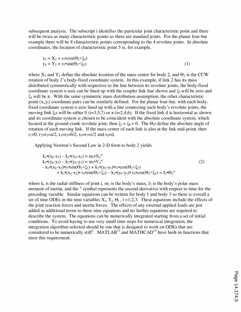
subsequent analysis. The subscript i identifies the particular joint characteristic point and there

will be twice as many characteristic points as there are standard joints. For the planar four-bar

example there will be 8 characteristic points corresponding to the 4 revolute joints. In absolute

coordinates, the location of characteristic point 5 is, for example,

x5 = X2 + r5•cos(e2+つ5)

y5 = Y2 + r5•sin(e2+つ5) (1)

where X2 and Y2 define the absolute location of the mass center for body 2, and e2 is the CCW

rotation of body 2’s body-fixed coordinate system. In this example, if link 2 has its mass

distributed symmetrically with respective to the line between its revolute joints, the body-fixed

coordinate system x-axis can be lined up with the coupler link line shown and つ5 will be zero and

つ4 will be ヾ. With the same symmetric mass distribution assumption, the other characteristic

point (xi,yi) coordinate pairs can be similarly defined. For the planar four-bar, with each body-

fixed coordinate system x-axis lined up with a line connecting each body’s revolute joints, the

moving link つis will be either 0 (i=3,5,7) or ヾ (i=2,4,6). If the fixed link d is horizontal as shown

and its coordinate system is chosen to be coincident with the absolute coordinate system, which

located at the ground-crank revolute joint, then つ1 = つ8 = 0. The eis define the absolute angle of

rotation of each moving link. If the mass center of each link is also at the link mid-point, then

r1=0, r2=r3=a/2, r4=r5=b/2, r6=r7=c/2 and r8=d.

Applying Newton’s Second Law in 2-D form to body 2 yields

k3•(x6-x5) – k2•(x4-x3) = m2•X2ギ

k3•(y6-y5) – k2•(y4-y3) = m2•Y2ギ (2)

- k3•(x6-x5)•r5•sin(e2+つ5) + k3•(y6-y5)•r5•cos(e2+つ5)

+ k2•(x4-x3)• r4•sin(e2+つ4) – k2•(y4-y3)• r4•cos(e2+つ4) = J2•e2ギ

where ki is the radial stiffness of joint i, m2 is the body’s mass, J2 is the body’s polar mass

moment of inertia, and the ギ symbol represents the second derivative with respect to time for the preceding variable. Similar equations can be written for body 1 and body 3 so there is overall a

set of nine ODEs in the nine variables Xi, Yi, ei , i =1,2,3. These equations include the effects of

the joint reaction forces and inertia forces. The effects of any external applied loads are just

added as additional terms to these nine equations and no further equations are required to

describe the system. The equations can be numerically integrated starting from a set of initial

conditions. To avoid having to use very small time steps for numerical integration, the

integration algorithm selected should be one that is designed to work on ODEs that are

considered to be numerically stiff3. MATLAB

13 and MATHCAD

14 have built-in functions that

meet this requirement.

Page 14.174.5

Figure 3 Planar Four-bar ICA Variables

As a sample numerical case, consider a planar four bar with a viscous rotational load of 10 N-

m/s acting on body 3 and a 2 KW nominal 1800 rpm induction motor (reduced by a 10:1 ratio

gear train) acting on body 1. The four-bar has a crank length of 0.1 meter, a coupler and

follower of lengths 0.4 meters each and a base length of 0.6 meters. The crank has a mass of 1

kg and J of 100 kg-m2. (The high crank J is because a flywheel has been included with the

combined crank, motor and gear train mass moments of inertia.) The coupler and follower each

have a mass of 4 kg and a J of 0.12 kg-m2. The bearings have a nominal commercial bearing

radial stiffness of 5e8 N/m. except for the coupler link bearings, which are rubber mounted so

their effective stiffness is 5e6 N/m.

For this example the nine equations of motion for the planar four-bar were numerically

integrated using MATLAB [13] ODE solver ode15s for 1 second of motion. The results are the

moving link mass center displacements and velocities and the link angular displacements and

velocities as a function of time. The joint reaction forces can be directly calculated from the

motion parameters. For example the horizontal joint reaction force at characteristic point 5

(Figure 3) is given by F65x = k3(x6-x5) where x5 is computed from the numerical integration

results using Eqn. (1) and x6 is similarly calculated.

Figure 4 shows that the variable inertia of the system causes the crank and input induction

motor velocity to slightly fluctuate. The constant voltage torque speed characteristics of the

drive motor are included in the model with the assumption that the torque-speed relationship is

linear in the range 1700-1900 rpm, the applied torque is a maximum at 1700 rpm, the applied

torque is zero at 1800 rpm, and the motor acts as a brake/generator at speeds greater than 1800

rpm. Figure 5 shows that the motor velocity fluctuations in Figure 4 are in synch with the

follower velocity fluctuations. Also Figure 5 shows that the abrupt startup, the initial conditions

which are only approximately consistent, and the bearing flexibility lead to an initial transient in

the follower angular velocity. Other than the initial transient, the ICA results for this example are

(X1,Y1,e1)

(X2,Y2,e2)

(X3,Y3,e3)

r5

e2+つ5

k3(y6-y5)

k3(x6-x5)

k2(x4-x3)

k2(y4-y3)

k1(y2-y1)

k1(x2-x1)

k4(x8-x7)

k4(y8-y7)

characteristic point 5 characteristic point 4

Crank, body 1

Coupler, body 2

Follower, body 3

Fixed base

Page 14.174.6

similar to the results from a conventional approach using exact initial conditions and ideal joint

behavior.

Figure 4 Planar Four-bar Crank Angular Velocity

Figure 5 Planar Four-bar Follower Angular Velocity

Vehicle Front Suspension Example

Figure 6 is a photograph of the front suspension of a 2008 Toyota Tundra. Figure 7 is a

schematic representation of this suspension. In addition to the fixed ground member, the

suspension has 7 moving bodies including the truck body. An eighth zero mass moving body

with a horizontal prismatic joint connecting it to the ground (and a revolute joint connecting it to

the tire at the contact patch center) needs to be added at the ground contact patch of the right

wheel to allow lateral sliding of that wheel with no resistance. This lateral free motion along the

ground corresponds to the situation where the vehicle is travelling freely down the road. (When

0 0.1 0.2 0.3 0.4 0.5 0.6 0.7 0.8 0.9 1179.701

179.702

179.703

179.704

179.705

179.706

179.707

179.708

179.709

179.71

Time [sec]

Cra

nk

An

g V

el [r

pm

]

0 0.1 0.2 0.3 0.4 0.5 0.6 0.7 0.8 0.9 1-50

-40

-30

-20

-10

0

10

20

30

40

50

Time [sec]

Fo

llo

we

r A

ng

Ve

l [r

pm

]

Page 14.174.7

the vehicle is stationary there is considerable lateral resistance due to friction between the tires

and the ground.) The other wheel is attached to the ground with a revolute joint at the center of

its contact patch. This left-right distinction is arbitrary and the ground contact conditions could

be reversed with no change in the analysis results. The other 8 joints can be considered revolute

joints. The suspension is held in its neutral position by preloaded springs which are located on

the same strut axes with the shock absorbers.

Figure 6 Tundra Front Suspension

Figure 7 Schematic of the Tundra Front Suspension

Figure 8 is a screen shot of the GUI input dialog that describes this suspension using the

author’s program ICAP. ICAP is a program written in MATLAB that uses the ICA to solve

Upper A-arm

Lower A-arm

Spring-shock Strut

Anti-sway bar

Page 14.174.8

planar mechanism problems. ICAP also has an automated GUI to support plotting of the

dynamic simulation results (Figure 9) or the user can further manipulate the resulting data (saved

by ICAP in a .MAT file) using standard MATLAB commands.

Figure 8 ICAP Input GUI for the Tundra Front Suspension

Figure 9 shows the vertical component of the force acting on the left lower arm to body joint

when travelling over a 0.1 m jump in road surface elevation. The solid line shows the response

when all the suspension joints are rigidly mounted with a nominal radial stiffness of 1e8 N/m.

The dotted line shows the response when the A-arm to body joints are all rubber mounted with a

radial stiffness of 5e5 N/m. The use of rubber mounts does not reduce the magnitude of the

bearing force. However the rubber mount response does not have the high frequency oscillations

superposed on its fundamental response as is the case for the stiff mounting. These force Page 14.174.9

Page 14.174.10

being a mechanical oscillator that is the source of a vibration problem. The ICA and ICAP are

thus basic tools that enable students and designers to more simply examine integrated

mechanism design and vibration problems.

Conclusion

The ICA provides a straightforward alternative method to determine the equations that

describe the motion and forces in a mechanical system consisting of rigid bodies connected by

standard joint types. One can visualize the ICA as using springs with certain characteristics

(corresponding to the joint type) to connect the bodies in the system being analyzed. Irrespective

of the initial conditions, these special springs will force the mechanism towards a minimum

potential configuration that corresponds to a completely assembled mechanism. The dynamic

equilibrium conditions can be written for each moving body using Newton’s second law, where

the joint reaction forces are expressed in terms of the six (or three for planar problems) basic

kinematic coordinates for each rigid body. The equations and unknowns for the problem are

simply six times the number of moving bodies (or three times for planar problems). Standard

ODE numerical integration routines can be used to solve the equations. The ICA can be applied

to problems where the joints behave ideally due to their high stiffness or to problems where the

joints are designed to be more flexible. The solution approach is the same in either case and is

generally simpler to implement than the conventional approach that uses kinematic loop

equations to constrain the basic dynamic equilibrium equations.

The ICA lends itself to being computer automated to handle arbitrary mechanism topologies.

The author has written such a program (using MATLAB) that can solve for the kinematic

properties and joint reaction forces for a planar mechanism of arbitrary complexity. The

mechanism can have multiple open and closed loops. GUIs are used to initiate the program,

provide the mechanism description and operating conditions and identify the outputs of interest.

The vehicle front suspension problem illustrates the use of this computer program.

References

1. Norton, R. L., Design of Machinery, McGraw-Hill, 2008.

2. Garcia de Jalon, J. and Bayo, E., Kinematic and Dynamic Simulation of Multibody Systems, Springer-Verlag,

1994.

3. Ascher,U. M. and Petzold, L. R., Computer Methods for Ordinary Differential Equations and Differential-

Algebraic Equations, Society for Industrial and Applied Mathematics, 1998.

4. Chace, M. A., “Analysis of the Time-Dependence of Multi-Freedom Mechanical Systems in Relative

Coordinates”, Transactions of the ASME, Journal of Engineering for Industry, Vol 89, No 1, Feb 1967, pp 119-

125.

5. Baumgarte, J., “Stabilization of Constraints and Integrals of Motion in Dynamical Systems”, Computer

Methods in Applied Mechanics and Engineering, Vol 1, 1972, pp 1-16.

6. Ascher,U., Chin, H., Petzold, L., and Reich, S., ”Stabilization of Constrained Mechanical Systems with DAEs and Invariant Manifolds”, Journal of Mechanics of Structures and Machines, Vol 23, 1995, pp 135-158.

7. MSC Adams, MSC Software Corp., Santa Ana, CA.

8. Reuleaux, F, The Kinematics of Machinery, MacMillan, 1876 (translation by A. Kennedy of 1875 German text);

also Dover, 1964.

Page 14.174.11

9. SimMechanics, MathWorks, Natick, MA.

10. Working Model 2D, Design Simulation Technologies, Canton, MI.

11. Marsh, E.R., and Yantek, D.S., “Experimental Measurement of Precision Bearing Dynamic Stiffness”, Journal

of Sound and Vibration, 201(1), 1997, pp 55-66.

12. Sutherland, G., “Mechanism Analysis Using Implicit Constraints”, Proceedings of the ASME International Design Engineering Technical Conferences, August 2008.

13. MATLAB, MathWorks, Natick, MA.

14. Mathcad, Parametric Technology Corp., Needham, MA.

Page 14.174.12