Journal of Research of the Na tional Bureau of Standards Vol. 51 , No.6, December 1953 Research Paper 2462

An Analogue Computer for the Solution of the Radio Refractive-Index Equation

Walter E. Johnson

The solution to the radio refractive-index equation provides information n ecessa ry to the research worker studying t ropospheri c radio propagation in t he ver y high and ultrahigh }·egions. Presen t means of computation are either t ime consuming or of low accu racy. An analogue co mputer is developed to solve t his equat ion by utilizing basic computation circuits incorporated in to a null-balance bridge circui t. A unique feat ure of this co mputer is the modification of a linear lO-t urn potentiometer so t hat its output to input voltage rat io versus rot ation closely approximates t he exponen tial-type curve of t he saturated water-vapor term in t he refractive-index equation .

This co mpu ter is now in use a t t he Cen t ral nad.io Propagat'ion Laboratory, of t he National Bmeau of Standards, Boulder , Colo., a nd has superseded Qther met hods of calcu­latin g t he radio refrac tive index.

1. Introductory Concepts

Analogue and digital computation devices are not only lightening the load of mathematicians and design engineers, but also are in many cases enabling the research workcr to explore problems that havc, in the past, been neglected b ecause of the volume of calculations required prior to embarking on th e analysis of the actual problem. Such a case exists in radio-propagation studies in the form of atmos­pheric refractive-index computations.

1.1. Development of the Basic Refractive-Index Equation

The two parts of the equation for the radio r e­fractive index a developed by D ebye [1] 1 arc: (a) a term proportional to density resulting from the

, induced polarization of the gas molecules in an external field ; and (b) a term proportional to th e permanent dipole moment of the molecules.

The latest m icrowave determinations of the con­stants of this eqnation yield the following ex­pression [2] :

N =(n - I )106= 7~6 (p+ 48~Oe} (1)

where N = refracti vity of air, n = refractivc index of air, T= absolute temperature in degrees K elvin, p = total pressure in millibars, e= partial preSS Ul'e of water vapor in millibars.

1.2 . The Refractive Index in Radio-Wove-Propaga­tion Studies

For low angles of elevation, the curvature of a radio ray is, to a high degree of approximation, equal to the gradient or change of refractive index with height. Consequently, the radio horizon fof VHF- UHF communications is determined solely by the refractive-index gradient. With an increase in

I Figures in bracketi indicate the li terature references &t the end of this paper.

335

the refractive-inclex gradient, the dis tance to the radio horizon frequ ently can increase fourfold and under extreme conditions may b ecome theoretically infinite. Therefore, a knowledge of the rcfractive­index profile with height would suffice for refrac­tion tudie:=;. If, however , one i concerned with reflection from elevated layers, then one needs the additional knowledge of the distribution of r efractive index throughout the layer.

In radio surveying and navigation studi e the absolute value of the refractive index is n eeded because of the fact that the velocity of electro­magnetic wave in air is inversely proportional to the refractive index.

For a typical propagation study, at least two Weather Bureau radiosonde 2 tations are selected , one on each ide of th e radio-transmission path. Each radiosonde records data at between 15 and 20 different elevations. For 1 year's radio data, there would be at least 21,600 calculations of N to be made for the two radiosonde station , taking obser­vations twice eaeh day. Therefore, i t can be seen that a great deal of time is consumed in laborious cal­culations prior to making a radio-propagation tudy.

1.3. Present Methods of Calculating the Refractive Index

One of the most common mean of reducing the calculating time is the utilization of nomogram. A recent example of the nomogram approach is that of Swingle [3], which utilizes a separate nomogram for each term in the refractive-index equation and has a maximum possible accuracy of ± 1 N unit. The solu tions that utilize a s ingle nomogram are never more precise than Swingle's method , and it is not uncommon to encounter errors of ± 5 N units.

Another approach to solving the equa tion is to use specially constructed slide rules . W eintrau b [4] utilizes 2 slide rules, 1 for each term in the refractive­index equation, and attains an accuracy of ± Yz N unit.

' The radiosonde is a measurin g system designed to measure the tempera­ture , pressure, and relative humidity of tho atmosphere at olevations from sea level to 100,000 ft above sea level.

A major factor to be considered is that both the nomogram and the slide-rule methods require the s trict attention of the calculator, and, as such, fa­tigue and the human element restrict not only the average accuracy of the results, but also the number of consecutive computations possible at one time. The time necessary to compute the separate terms in the refractive index and the subsequent addition varies from approximately 30 sec, using slide rules, to from 30 to 45 sec, using nomograms.

The material to follow describes a relat ively sim­ple electric analogue computer that has been designed to solve this equation.

2 . Computer Requirements

The general requirements that a computer designed to solve this equation must meet are much the same as those that would be placed on any computer. An ideal approach to the problem would be to make the computer as accurate, as fast, and as convenient as possible. However , i t would be well to take a more realistic approach toward finding practical limits to each of these three requirements.

2 .1. Accura cy

In general, the computer accuracy need be nogreater than is consistent with the accuracy of the available data to be used. Striving for gr eater accuracy would only lead to greater expense and perhaps undue com­plications in the circuits. However , the possibility that the accuracy of the available data may at some future date be increased must be taken into account.

At present, the greater part of the available meteorological data has been obtained from r<l.dio­sonde ascents. The accuracies associated with these data would dictate a computer accuracy of no greater than 1 or 2 N units of refractivity. However, future plans indicate that some of the data will be obtained from relatively accurate recording instruments placed at discrete elevations on specially located steel towers. To accurately solve the refractive-index equation, using data obtained in this manner, it. will be neces­sary to specify an accuracy of ± % N unit .

2 .2 . Speed

A very obvious limitation on the overall time required to complete one computation is that the total time can be no less than the time required to supply information to the computer , which is propor­tional to the variables in the equation. This is commonly referred to as the "setup" time. In operation, the operator will be required to read data sheets, which have temperature, pressure, and rela­tive humidity recorded as numerical values and introduce this information into the computer. Using either of the two more common media of dials or pushbuttons, it would appear well to allow at least 3 sec for each of these operations. Allowing another 3 sec to complete the solution wo.uld indicate a figure

of approximately 12 sec to obtain one solution with the computer. This figure , if met by the computer , would be a considerable improvement over the speed -obtained by either the nomogram or the slide rules.

2.3 . Convenience

In designing a computer of this type, which must perform a large number of similar computations, too much stress canno t be laid on its convenience of operation. A machine that has been designed with this in mind no t only speeds up the operational time for the operator, but also gl"eatly reduces operational errors. Oertain general features emerge from a care­ful consideration of the convenience requirement.

The dials or pushbuttons used to introduce the variables should be arranged in the same relative order as the da ta on the data sheets . Also they should be convenient to read and should be calibrated in the same units as the Ol"iginal data. The method of reading the answer should be such that the opera­tor may r ead and record the result from the same , convenient position as used to set up the computer.

With these general requirements in mind, let us next investigate the basic electric circuits that will be required in an electric analogue computer designed to solve the refractive-index equation.

3. Basic Computation Circuits

If the constants 77 .6 and 4810 in eq. (1) are re­placed by K I and K 2, respectively, and e by its equiva­lent, e,RH, the saturated vapor pressure times the relative humidity, the equation will now appear as

(2)

It is to be noted that fOl' the present e,/T will be co_nsidered as a variable, as are T, p, and RH. The discussion to follow describes the method used to eliminate e,/T as an independent variable and thus reduce to three the number of variables that must be introduced into the computer.

Inspection of the equation reveals that multiplica­tion must be accomplished in obtaining the product K2 (e, IT )RH . Addition is next used to add p to this product , and finally, division is utilized to divide this binomial by TIK I' The circuits to follow indi­cate how each of these three mathematical operations may be duplicated electrically. In each of these circuits et represents a d-c voltage source, with zero internal impedance, and eo is the output voltage, as measl!r ed with an infinite impedance voltmeter. The variable-resistance symbols represent linear potenti­ometers so designed that the voltage as measured at the slider is equal to the percentage rotation times ' the voltage applied to the potentiometer . X is used to represent the percentage of total rotation as measured in the direction of the small arrow asso­ciated with X.

336

FI G URE 1. 111{ ulti plication ci,·cui t.

3 .1. Multiplica tion

The circuit shown in figure 1 is presented as a method of multiplying two variables by a constant. The equation that expresses the ratio of output vol tage to input voltage in this circui t is

If R3»Rz, the equation 3 may be simplified as follows:

eo R2 XX - = R + R 2 3· et 1 2

(3)

This equation shows that when R 2/ (R1+ R2) is made equal to the desired constant and X 2 and Xa equal to the variables, the voltage ratio , eole!, will equal the product of the constant and the two variables.

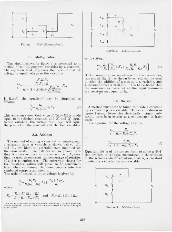
3 .2 . Addition

The method of adding a constant , a variable, and a constant times a variable is shown b elow. R49. and R4b are identical potentiometers mounted on the same shaft . Their sliders are so phased that they both are on zero at the same time. X 4 may then be used to represent the percentage of rotation of either potentiometer. The subscripts chosen for the resistance values will prove to be convenient later when combining th e basic circuits into the combined computation circuit .

I The ratio of output to input voltage is given by

where

3 When R, is 200 times R" the solu tion obtaiued by eq (3) shows a maximum error in eo/e, of 0.07 percent. This maximum error occurs at a value of X , equal to 66.7 percent.

R4b t I

RI Rs ' X4

t ej Rz e

R4a t I

j I Xz

R6a

FIGURE 2. Addition circuit.

or, rewriting,

If the correct values arc chosen for the resistances, this circuit (fig. 2 ), a shown by eq (4), can be used to solve the addition of a constant, a variable, and a con tant times a variable. It is to be noted that the resistance as measured at the input terminals is a constant and equal to R •.

3.3. Division

A method must next be found to divide a constan t by a constant plus a variable. The circuit shown in figure 3 accomplishes this electrically. Again, sub­scripts have been cho en as a convenience to la ter work.

The equation for the voltage ratio is

eo R. ei R.+R7+ X5R5

or eo R.IR5

ei (R.+R7)/R5+,X 5 (5)

Equation (5) is of the proper form to solve a divi­sion problem of the type encountered in the solution of the refractive-index equation, that is, a constan t divided by a constant plus a variable.

1 R5 ~ . t

] X5

ej R7 e

Rs

F IGURE 3. Division circuit.

331

4. A Circuit to Solve the Refractive-Index Equation

4 .1 . Limits on the Va riables

Before proceeding to combine the three basic cir­cuits, it will be well to investigate each variable separately in the equation and discover the limits that may be placed on each of them. In addition, the variables in the equation must be modified so that they may be interpreted as the X variables as used in the basic circuits. This requires that the maximum value of each variable be referred to a value of unity, and as such can be made equal to a percentage of rotation as expressed by the X vari­ables. Consideration will also be given toward estab­ishing limits on the variables such that standard

dials graduated (or marked) with 10 major divisions to the revolution may be used.

The temperature, T , as found in the equation, represents the absolute temperature and may be written as 273 + t, where t is in degrees centigrade. Because the data obtained from the recording instru­ments are in terms of degrees centigrade, it will be more convenient to have the dial marked in these same units. Investigation of the data · eurrently available disclosed that temperatures to be encoun­tered will lie between ± 50° C. This range permits each revolution of a 10-turn potentiometer to rep­resent a change of 10 deg, and the dial can be marked to read zero at its midscale position. With regard to the circuit, the temperature expression may be rewritten T = 100(2.23 + X T ). As a check on the validity of this expression, consider the absolute temperature at 0° C. X T , or the fractional rotation, would equal 0.5, and the expression would give an absolute temperature of 273° K, as was to be expected.

Initial investigation of the pressure variable indi­cated that a range of 0 to 1,000 millibars would be adequate to accommodate all the current and future data. However, closer checks revealed that a range of 100 to 1,100 millibars would be more suitable. This range still permits assigning 100 millibars to each revolution of a 10-turn potentiometer, but re­quires that a constant be added to the circuit to take account of the 100-millibar shift. The expres­sion for p is written p = l ,OOO(O.l + X p ). Here again Xp is the percentage of dial rotation, with the dial calibrated from 100 to 1,100 millibars. As an ex­ample, with the d ial set for 600 millibars , X p would equal 0.5 , and p would equal 600.

The relative-humidity variable lends itself ad­mirably to expression as a percentage rotation. Because it varies from 0 to 100 percent in the same manner as the X variable, the dial may be grad­uated 0 to 100 and used directly . . Investigation of the data disclosed that the complete range 0 to 100 would be required to accommodate all the data.

Although the es/T variable will later be eliminated as an independent variable, its limits will be con­sidered at this time. Using the 1951 Smithsonian

338

Meteorological Tables [5], e,/T was found to vary from 0.0003 at - 50° C to 0.3820 at + 50° C. In order to use all the available rotation of a linear potentiometer, it will be necessary to express the variable as 0.3820 X es/T and use a speciallv marked dial to position the slider of the potentiometer.

4.2 . The Basic Circuits Combined

With the above information in mind, eq (2) may be rewritten

N 100 (2,~ +XT) [1000(0.1 + X p )+ 0.3820X(e,/ T)X RH]

or

N=2.~~!XT [ 0.1 + X p + 0.3820 1~~OX(e8 f T) XRH J The basic circuits will now be combined, and it will be shown that, by properly selecting the resistance values, the combined circuit can be used to solve the refra?tive-index eq~ation in the form of eq (6).

Usmg the equatIOns already established for the basic circuits, the equation for the combined circuit of figure. 4. ~ay ~ow .b~ writt~n. The output voltage of the (hVIs~o.n CU'?UIt .IS apphed as the input voltage to the addItIOn ClrcUIt, and the variable X 3 is in­cluded in the last term of the equation for the addi­tion circuit. Justification for this action is found by comp~ring the multiplication circuit of figure 1 with the nght-hand portion of the addition circuit of figure 2.

The equation for the ratio of voltages in figure 4 is

Rs

Rr

R4b ej eo

Re' R3

X3 R40

Rso

FIGURE 4. Combined computation circuit.

A comparison of eq (6) and (7) will show the sim­ilarity of the two equations. It is now only necessary to equate the resistance combinations in eq (7) to the constants in eq (6). The output to input vol tage ratio is then equal to N.

5. Elimination of es/T as an Independent Variable

Up to this point es/T has been considered as a separate variable in the equation. The curve plotted in figure 5/ shows that es/ T has explicit dependence on the temperature. This fact can be used to eliminate es/T as an independent variable and consequently reduce the setup time for the computer.

As discussed in section 4.1., if a linear potenti­ometer is to be used to introduce the es/T ratio , its dial must have a special marking. The sam e ratio may be established by using a linear dial and a poten tiometer with an output function tha t matches the curve in figure 5. Unfortunately, the curve cannot be duplicated by any convenient mathe­matical expression. However, it is possible to ap­proximate the curve by a series of straigh t lines con­necting the circled points on figure 5. Although this approach does no t yield a perfect solution at all points, th e accuracy can be made as high as required by merely increasing the number of straigh t-line approximations.

A method known as resistance loading, or " pad­ding", was used to alter the normally linear ou tpu t of a 10- turn potentiometer . This linear relationship between resistance and shaft rotation can be altered

POTENTIOMETER ROTATION, DEGREES

o 360 720 1080 1440 1800 2160 2520 2880 3240 3600 0.40 .----.----r---r--y--,--r----.----r---r--,

0.35

0.30

0.25 I-';;;. ., 0 .2 0

0 . 15

0.10

0.05

o L--L __ ~~~~~L-_L __ ~~ __ _L~ -50 -40 - 30 -20 -10 0 10 20 30 40 50

TEMPERATURE, · C

FIGURE 5. e./ T versus temperature. Theoretical cun'e shown by the solid line, actual oUipui funciion shown by the

circles. ell js the saturation vapor pressure in millibars; T is a bsolu te temperature.

• Data for this CUITe were taken from the 1951 Smithso nia n Meteorological Tables [.5].

27D6S3- 54--3 339

by connecting padding re istors between tap points on the poten tiometer coil so that the output will vary in a close approximation to Lhe des ired function. By properly choosing the resistance of the pads, the straight lines generated between the tap points can be made to cross the desired curve at two points. The number of tap points was chosen so that at no point would the series of straight lines deviate from the theoretical enough to contribu te over iN uni t error to the final resul t.

Examination of the curve disclosed that taps located at the following d egree positions would provide for the desired accuracy: 81 0, 1260, 1530, 1800, 2070, 2340, 2610, 2880, 3150, and 3420. A 2,000-ohm potentiometer was selec ted for this modification, as 2,000 ohms was the lowest resistance, commercially available, lO-turn po tentiometer tha t could be obtained for this purpose. Approximate resistance values were calculated to pad the 2,000-ohm potentiometer to the desired points on the curve, and it was found possible to hold the total resistance after padding to 200 ohms. The exact values of the padding r esistances were determined by the voltage-comparison m ethod described below.

A 500-ohm 10-turn potentiometer wa placed in series wiLh the tapped potentiometer R2• A voltage was appli ed to the series combination, and Lhe output voltage at the slider was read, po ten tiom eter type precision voltmeter. The ratio of slider volt­age was calculated for each tap point, and , starting from the lowest tap point, th e values of the padding resistors were adj usted to m ake the voltage ratio check exactly with the desired value of es/T. The 500-01un po ten tiometer was adjusted after every change in padding resistance so as to keep the total series resistance constan t and equal to 523.5 ohms. Because the maximum value of es/ T was to be 0.3820, the 500-ohm po tentiometer was replaced by a fixed resistance (RI ) of 323.5 oluns upon com­pletion of the padding operation.

This m ethod provided much greater accuracy than could have been obtained by calculating the values for the padding resi tors. With the type of precision voltmeter used, it was possible to read the voltages to five-figure accuracy, and consequently the resistors could be changed to permit adjusLing the voltage ratios at the tap points to an accuracy of 0.01 percent. ~Wire-wound resistors of the same temperature coefficient wire as that used in the potentiometer were specially constructed for this purpose.

Using the potentiometer just described, it is now possible to graduate its dial from - 50 0 C to +500 C in exactly the same manner as the temperature dial. In fact, the dial can now be eliminated and the es/ T potentiometer can be connected directly to the shaft of the temperature potenLiometer. This has in effect eliminated the cs/T variable, in that it now depends directly on the temperature dial for its setting.

6 . Final Design Considerations

6 .1. Choice of Solution Presentation

As shown by eq (7), the computation circuit as developed to this point will provide a solution to the refractive-index equation in the form of a voltage ratio. A more convenient and accurate method of presenting the solution is to combine the composite circuit of figure 4 into a bridge circuit and use a sensitive null indicator to detect the bridge balance. Figure 6 shows the complete computer circuit dia­gram. Potentiometer Rg and the fixed resistance RIO constitute one arm of the bridge, and the com­bined computation circuit of figure 4 forms the other arm. Rg is the same type lO-turn linear poten­tiometer as used to introduce the variables. A linearly calibrated dial attached to Rg was used to read N directly. RIo is a wire-wound resistor, as are all the other fixed resistances.

The null indicator used is of a special design having a maximum sensitivi ty of X-in. motion per microampere at about the zero position. Its response falls off logarithmically on either side of zero and thus provides automatic protection against excessive currents caused by large unbalances in the bridge circuit.

6.2. Selection of Resistance Values

R eferring to figure 6, the following expression for the voltage as measured at the slider of Rg may be written:

eo X gRg C; Rg+ RIO' (8)

With the circuit as shown at null balance, this expression may be equated to eq (7).

R4a(Rg + RIO)

X g= R5R9 [R6a+ x 4+ . --.!}pRz - X2X3J . (9) R,,+ R7 + X5 R4a R4.(RI+ Rz)

"" PI to! Lamp

R5

.11 800

.5 500 I

I

(~~;,~F 5~; L---------r:,"

1 ~~:;-----t--,~--, = 90Volt I

~ ~~~ ~:~+---+ _____ l ~_-----.J FIGURE 6. Computer-circuit diagram.

I I I

©

.9 500

Bo th sides of this equation must be multiplied by 1,000 to permit solving for values of N up to 1,000. Investigation of the actual data disclosed that all the values of N will be between 0 and 1,000. The dial attached to Rg must therefore be graduated from ° to 1,000. Comparison of eq (6) and (9) requires that the following identities be satisfied in order to utilize the final circuit to solve the refractive-index equation:

1000 R4a(Rg + RlQ) R5R9

lOk i = 77 6· (10)

(R,+ R7) 2.23· (11) R5

R6a= 0.1. R4a

(12)

RpR2 K2 R4a(RI+ R2) . 10000.3820 = 1,8374. (I 3)

also R = (Rl + R2) (R4a +R~) .

p RI +R2+R4a+R~ (14)

Rs = Rp + R4a + R6a • (15)

There exist several combinations of the above resistances that will satisfy the above identities. The variable resistances or potentiometers must first be chosen on the basis of commercially available values. In general, they were chosen as small as possible in order to keep the over-all internal resist­ance of the circuit low with regard to the internal impedance of the null indicator. Low circuit resist­ance is necessary in this case to maintain sufficient sensitivity of the null indicator.

R4a and R4b were chosen as 100 ohms each. This value, by eq (12), required that R 6a = 10 ohms, which was still of a size tha t could be conveniently wound . R l and R2 have already been determined as 323.5 and 200 ohms, respectively. These values and the value for R4a when substituted in eq (13) give a value for R p of 481.00 ohms. Substituting this value in eq (14), along with the values for E l , R2, and R4a ,

gives a value of 5,825 ohms for R~. Solving eq (15) gives a value for Rs of 591.00 ohms. Equation (11) was next investigated in order to determine a value for R5. As R7 cannot have a negative value, R5 must be at least 278 ohms. The closest commer­cially available value of 500 ohms was chosen for R5 •

Using this value for R5, eq (11 ) was solved, and R7 was found to be 524.0 ohms.

Equation (10) was next used to determine the rela­tive magnitude of Rg and RIO. Solving this equation established the relationship

R9 Rg+ R lO = 0.25773 .

Rg+ RIO was chosen to be approximately 2,000 ohms so that excessive current would not be drawn from

340

the voltacre so urce and yet not be so great as to cause serious lo~s of sensitivity at the null indicator. This value for Rg+ R IO would indicate a value for Rg of about 515 ohms. A resistance of 500 ohms was chosen for R9 because resistors of that value are com­merciallyavailable. This choice for R9 required that R IO equal 1,440 ohms. R3 \~as selected ~s 50,000 ohms in order to satisfy the prevlOusly estabhshed relatlOn-ship that R3 b e at least. 200 times 1jl2'. .

Figure 6 shows a resIstan ce R ll III sen es WIth the battery supply voltage. Th)s resis.tor was used to reduce the bridge voltage to approxlffiately 50 volts. At higher voltages a slight h eating effect, alo~g with corresponding resistance changes, was noted III some of the resistors .

6.3. Wet- and Dry-Term Switches

The refractive-index equation may be considered as beincr composed of two parts, a wet term equal to K lr!(I{2RHes/T) and a dry term equal to (K d T)p. M any of the applications that requiTe the S.olu tlOn of the refractive-index equa tion also reqUIre the values for eitll er the wet or dry con tribution to N. Two swi tches were incorpora ted into the linal circui t, which permit the computer to solve for either con­tribu tion and t hereby grea tly increa e the usefuln ess of the computer . .

In fig LU"e 6, R~ has been divided to form Rs and RM .

R 6b has been m ade equal ~o 10 ohms and Ijls equal to 5,815 ohms, th ereby keeplllg the total reslstance th e same. With t he switch connection between R 6b and Rs closed, the pressure ter",? is efrectiv~ly reduced to zero and the computer, after rebalancmg, r eads the wet 'term. In a similar manner , closing the dry-term swi tch, effectively makes the wet term zero, and th e compu ter solves for the dry term only.

7. Results and Discussion

The computer herein described was built under the author's supervision at the. N ational Bure~u of S~and­ards, Boulder , Colo ., and IS at pre en t belllg actlvely used by their Radio Meteor~logy G:roup. The use of the computer has resulted III consIderable avings in time over previously used methods.

7.1. Accuracy

A complete test was run on the computer, and the results of this test are given in table 1. The table shows that the error is never greater than ± t N uni t. This satisfies t he original requirement. If greater accuracy were to be required,. a greater number <?f tap points on ~he e.s/T po ten tlOD?-eter would permI t a closer approXlmatlOn to the desll'ed curve and con­sequently increase the final accuracy. The need for greater accuracy woul~ also necessitate the usc of dials with finer graduatlOns.

341

T,unE 1. Final test data

N 'rempera- Pressure Relative

ture humidity 'rheorcticai Computer

------° c i\1illibar 8 -50 100 0 34. 80 34. 6 -50 1, 100 0 382.78 383. 1 + 50 100 0 24.02 24. 0 +50 1,100 0 264. 27 264. 6 +50 100 100 465. 51 465. 7 + 50 1, 100 100 705. 75 706. 2

0 600 50 185. 86 185. 8 - 14 600 50 185.53 185.5 -12 600 50 185. II 185. 2 - 10 600 50 184. 77 184.9 + 40 600 50 289. 29 289. 7 + 42 600 50 302.27 302.6 + 44 600 50 315. 96 315.9 + 46 600 50 331. 00 330.7

,

7 .2. Speed

The average operational time of the computer and operator was found to be approximately 10 sec, which is less tha n the original req uil'emen t of 12 sec. This t ime naturally varies wi th the individual operator. The shortest time of 8 sec was re?orded for an experienced operator and the longest tIme of 13 sec was recorded fo r a relatively inexperienced operator. This time co uld be decreased somewhat by using an au tomatic balance sys~em to. rot.ate the N dial and thereby balance the bnclge W'CUIt more rapidly than can be dOl~e manually. This refinement was no t deemed practIcal for the present computer due to the relatively longer time required to set in the variables.

7.3. Convenience

All of the original requirements on convenience have been incorporated in the final design. Figm·.e 7 shows the computer. It is hOLlsed in a small slopmg

FIGUlm 7. Refractive-index computer.

front cabinet that can be placed on a desk or table and used in the same manner as a standard calculat­ing machine. Because of heating effects, it was found desirable not to leave the battery connected to the bridge circuit continuously. Withlthis in mind, a foot switch was incorporated in the final design so that the operator could energize the circuit as needed and still have both hands free to operate the dials and record data.

In figure 7 the various dials are set up to solve for N, with the temperature, 32.0° C; pressure, 620 millibars; and RH, 62 .5 percent. N is read as 277.0.

8. References

[1) P . D ebye, Polar molecules, sec. 3.4 (Chemical Catalog Co., New York, N. Y., 1929).

[2) E. Ie Smith, Jr ., and S. Weintraub, The constants in the equation for atmospheric ]'efractive index at radio fre­quencies, J . R esearch NBS 50, 39 (January 1953) RP2385.

[3) D . M. Swingle, Nomograms for the computation of tropo­spheric refractive index, Proc. IRE [3) 41, 385 (March 1953) .

[4) S. Weintraub, Slide rule for t he computation of the radio refractive index of air, Electronics [1) 26, 182 (January 1953).

[5) Smithsonian meteorological tables, 6th revised ed., p. 351- 352 (Smithsonian Inst., Washington, D. C., 1951).

BOULDER, COLO., July 13, 1953.

342