Embed Size (px)
Citation preview
University of South FloridaScholar Commons
Graduate Theses and Dissertations Graduate School
January 2013
An Analysis of Factor Extraction Strategies: AComparison of the Relative Strengths of PrincipalAxis, Ordinary Least Squares, and MaximumLikelihood in Research Contexts that Include bothCategorical and Continuous VariablesKevin Barry CoughlinUniversity of South Florida, [email protected]
Follow this and additional works at: http://scholarcommons.usf.edu/etd
Part of the Educational Assessment, Evaluation, and Research Commons, and the QuantitativePsychology Commons
This Dissertation is brought to you for free and open access by the Graduate School at Scholar Commons. It has been accepted for inclusion inGraduate Theses and Dissertations by an authorized administrator of Scholar Commons. For more information, please [email protected].
Scholar Commons CitationCoughlin, Kevin Barry, "An Analysis of Factor Extraction Strategies: A Comparison of the Relative Strengths of Principal Axis,Ordinary Least Squares, and Maximum Likelihood in Research Contexts that Include both Categorical and Continuous Variables"(2013). Graduate Theses and Dissertations.http://scholarcommons.usf.edu/etd/4459

An Analysis of Factor Extraction Strategies: A Comparison of the Relative Strengths of
Principal Axis, Ordinary Least Squares, and Maximum Likelihood in Research Contexts
that Include both Categorical and Continuous Variables
by
Kevin B. Coughlin
A dissertation submitted in partial fulfillment of the requirements for the degree of
Doctor of Philosophy Department of Educational Measurement and Research
College of Education University of South Florida
Major Professor: Jeffrey D. Kromrey, Ph.D. Robert F. Dedrick, Ph.D.
John M. Ferron, Ph.D. Constance V. Hines, Ph.D.
Waynne James, Ed.D.
Date of Approval: March 4, 2013
Keywords: Communality, Exploratory Factor Analysis, Factor Loading, Monte Carlo, Matrices of Association, Multivariate Normality, Overdetermination, Repeated Measures,
Sample Size, Scale Coarseness
Copyright © 2013, Kevin B. Coughlin

Dedication
This dissertation is dedicated to my wife, Deanna, and my children: Melia, Imriel,
and Jeremiah. Without their patience, tolerance, and support, I would not have
completed my course of studies or this dissertation. My wife and children have taught
me how strong and resilient a family can be, and, for this, I will always be thankful.

Acknowledgments
As I pursued my course of studies and completed this dissertation, I benefitted
tremendously from the guidance of my major professor, Jeffrey D. Kromrey, Ph.D. I will
always appreciate Dr. Kromrey’s capacity to provide excellent advice in a manner that
enabled me to make progress without making me feel as if I had been given the answer.
Without Dr. Kromrey’s assistance, I am not certain that I would have completed this
study. I would also like to thank Dr. Robert F. Dedrick, Dr. John M. Ferron, Dr.
Constance V. Hines, and Dr. Waynne James for serving on my committee and providing
me with voluminous and excellent feedback on my many dissertation drafts.
In pursuing my degree, I benefitted from the support and flexibility of my
colleagues and supervisors. Specifically, I would like to thank Dr. Frank Hohengarten
who supported my efforts to pursue a full-course load while serving on his staff. I would
also like to thank Dr. Steve Atkins, Dr. Erin Harrel, and Dr. Jeff Stewart for providing me
with encouragement and support as I completed this dissertation.

Table of Contents
i
List of Tables iv List of Figures ix Abstract xiv Chapter One: Introduction 1 Statement of Problem 2 Theoretical Framework 3 Purpose of the Study 9 Objective 9 Rationale 9 Supporting Examples 11 Research Questions 15 Hypotheses 16 First hypothesis 16 Second hypothesis 17 Significance of the Study 17 Definition of Terms 18 Delimitations 21 Organization of Remaining Chapters 22 Chapter Two: Literature Review 23 Exploratory Factor Analysis Design Considerations 23 Model selection 23 Samples of subjects 25 Samples of variables 26 Scale coarseness and dichotomization 27 Non-normal models 29 Matrices of association 31 Number of factors retained 36 Rotation 38 Factor Extraction Methods 40 Principal axis factor analysis 42 Ordinary least squares 44 Maximum likelihood 45
ii
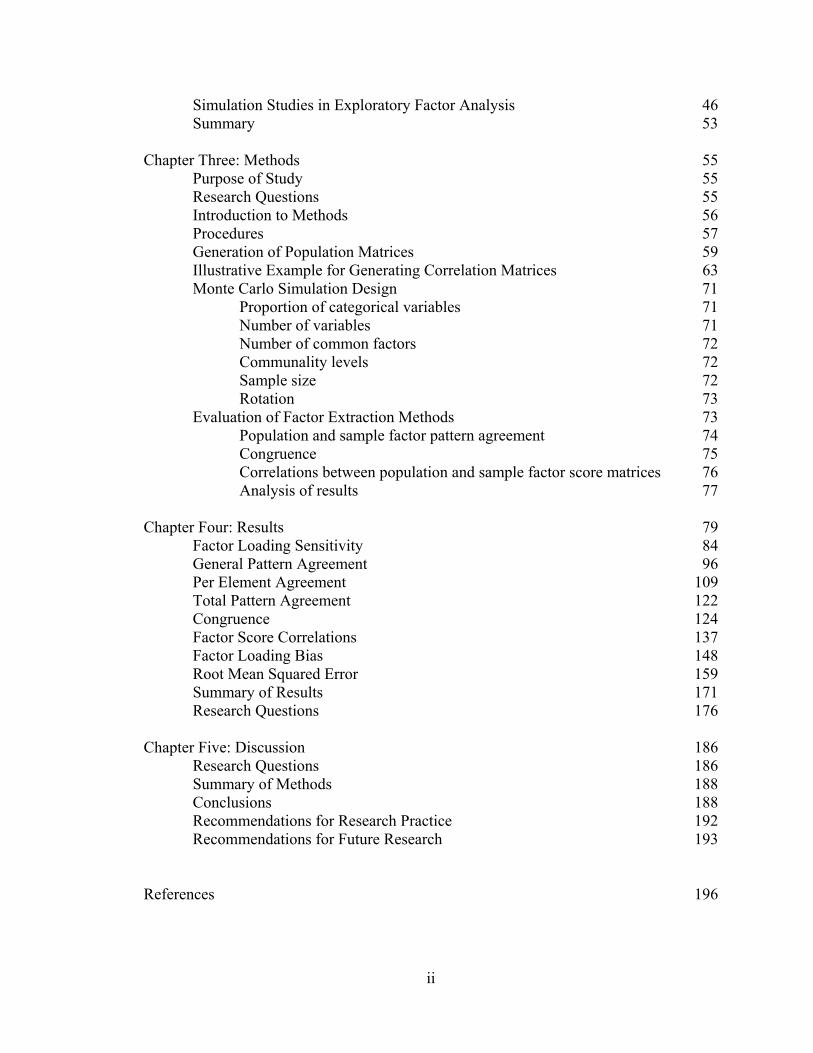
Simulation Studies in Exploratory Factor Analysis 46 Summary 53 Chapter Three: Methods 55 Purpose of Study 55 Research Questions 55 Introduction to Methods 56 Procedures 57 Generation of Population Matrices 59 Illustrative Example for Generating Correlation Matrices 63 Monte Carlo Simulation Design 71 Proportion of categorical variables 71 Number of variables 71 Number of common factors 72 Communality levels 72 Sample size 72 Rotation 73 Evaluation of Factor Extraction Methods 73 Population and sample factor pattern agreement 74 Congruence 75 Correlations between population and sample factor score matrices 76 Analysis of results 77 Chapter Four: Results 79 Factor Loading Sensitivity 84 General Pattern Agreement 96 Per Element Agreement 109 Total Pattern Agreement 122 Congruence 124 Factor Score Correlations 137 Factor Loading Bias 148 Root Mean Squared Error 159 Summary of Results 171 Research Questions 176 Chapter Five: Discussion 186 Research Questions 186 Summary of Methods 188 Conclusions 188 Recommendations for Research Practice 192 Recommendations for Future Research 193 References 196

iii
Appendix A: Technical Descriptions 201 Pearson Product Moment Correlation Coefficient 201 Spearman Rank Correlation Coefficient 201 Phi Coefficient 201 Tetrachoric Correlation Coefficient 202 Point-Biserial Coefficient 202
Partition Maximum Likelihood Model for Estimating Polyserial Correlation Coefficient 203 Two Stage Estimation of Polyserial and Polychoric Correlation 204 Principal Axis Factor Analysis 206 Ordinary Least Squares Factor Analysis 213 Maximum Likelihood Factor Analysis 216
Appendix B: SAS IML Code for Illustrative Examples 221 Appendix C: Multivariate Analyses of Variance Summary Tables 224 Appendix D: Box and Whisker Plots 248 Appendix E: SAS IML Code for Simulation Program 280 Appendix F: SAS IML Code for Data Analysis 298
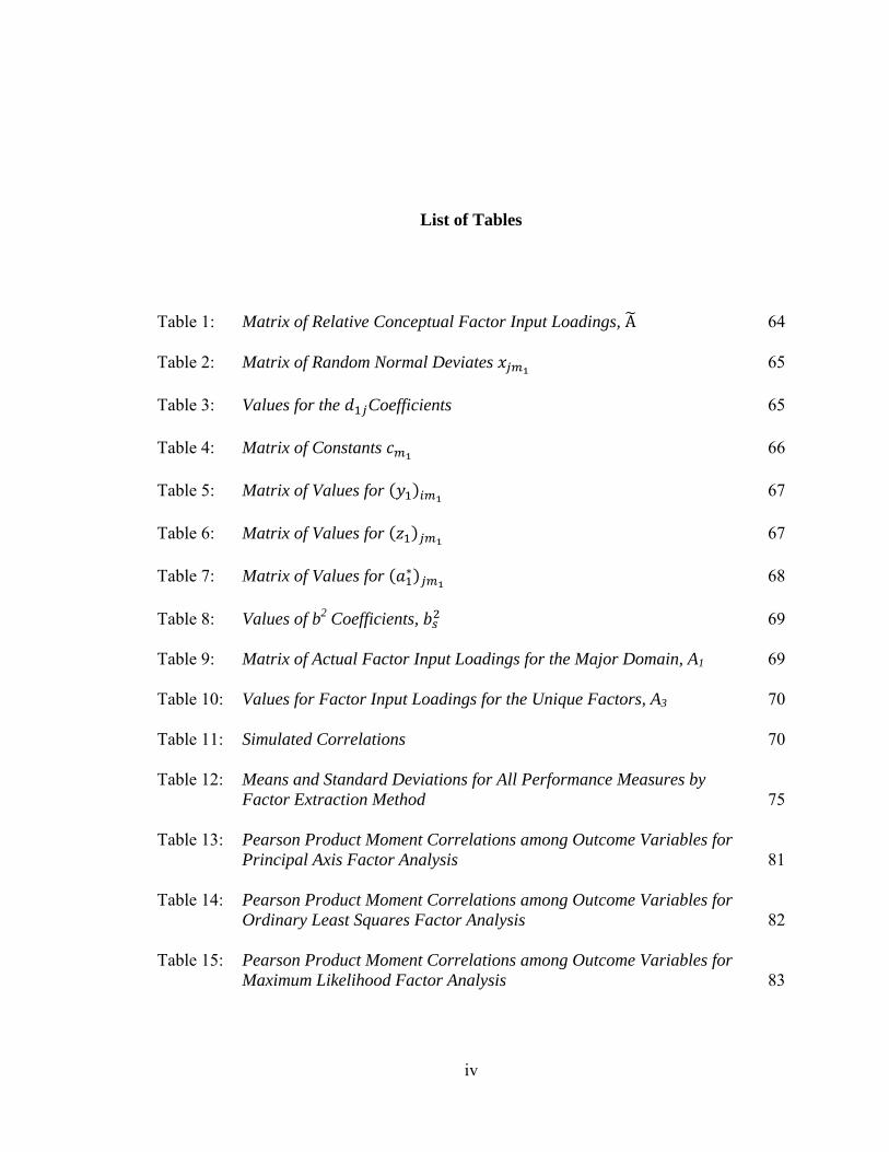
List of Tables
iv
Table 1: Matrix of Relative Conceptual Factor Input Loadings, A 64 Table 2: Matrix of Random Normal Deviates 65 Table 3: Values for the Coefficients 65 Table 4: Matrix of Constants 66 Table 5: Matrix of Values for 67 Table 6: Matrix of Values for 67 Table 7: Matrix of Values for ∗ 68 Table 8: Values of b2 Coefficients, 69 Table 9: Matrix of Actual Factor Input Loadings for the Major Domain, A1 69 Table 10: Values for Factor Input Loadings for the Unique Factors, A3 70 Table 11: Simulated Correlations 70 Table 12: Means and Standard Deviations for All Performance Measures by
Factor Extraction Method 75 Table 13: Pearson Product Moment Correlations among Outcome Variables for
Principal Axis Factor Analysis 81 Table 14: Pearson Product Moment Correlations among Outcome Variables for
Ordinary Least Squares Factor Analysis 82 Table 15: Pearson Product Moment Correlations among Outcome Variables for
Maximum Likelihood Factor Analysis 83

v
Table 16: Descriptive Statistics for Distributions of Factor Loading Sensitivity 84 Table 17: Means and Standard Deviations of Factor Loading Sensitivity by Factor Extraction Method and Number of Factors by Number of Observed Variables Interaction (K x P) 87 Table 18: Means and Standard Deviations of Factor Loading Sensitivity by
Factor Extraction Method and Number of Factors by Communality Range Interaction (K x H) 90 Table 19: Means and Standard Deviations of Factor Loading Sensitivity by
Factor Extraction Method and Number of Factors by Level of Dichotomization Interaction (K x D) 92
Table 20: Means and Standard Deviations of Factor Loading Sensitivity by Factor Extraction Method and Number of Observed Variables by Communality Range Interaction (P x H) 94 Table 21: Descriptive Statistics for Distributions of General Pattern Agreement 97 Table 22: Means and Standard Deviations of General Pattern Agreement by Factor Extraction Method and Number of Factors by Number of Observed Variables Interaction (K x P) 100 Table 23: Means and Standard Deviations of General Pattern Agreement by Factor Extraction Method and Number of Factors by Communality Range Interaction (K x H) 102 Table 24: Means and Standard Deviations of General Pattern Agreement by Factor Extraction Method and Number of Observed Variables by Communality Range Interaction (P x H) 105 Table 25: Means and Standard Deviations of General Pattern Agreement for Factor Extraction Method and Sample Size by Communality Range Interaction (N x H) 107 Table 26: Descriptive Statistics for Distributions of Per Element Agreement 110 Table 27: Means and Standard Deviations of Per Element Agreement for Factor Extraction Methods by the Number of Factors and Number of Observed Variables Interaction (K x P) 112 Table 28: Means and Standard Deviations of Per Element Agreement for
Factor Extraction Method and number of Factors by Sample Size Interaction (K x N) 114

vi
Table 29: Means and Standard Deviations of Per Element Agreement for
Factor Extraction Method and Number of Factors by Communality Range Interaction (K x H) 116
Table 30: Means and Standard Deviations of Per Element Agreement for
Factor Extraction Method and Number of Variables by Communality Range Interaction (P x H) 118 Table 31: Means and Standard Deviations of Per Element Agreement for
Factor Extraction Method and Sample Size by Communality Range Interaction (N x H) 121
Table 32: Descriptive Statistics for Distributions of Total Pattern Agreement 123 Table 33: Descriptive Statistics for Distributions of Congruence 125 Table 34: Means and Standard Deviations of Congruence Values for Factor Extraction Method and Number of Factors by Observed Variables Interaction (K x P) 127 Table 35: Means and Standard Deviations of Congruence Values for Factor Extraction Methods and Number of Factors by Sample Size Interaction (K x N) 129 Table 36: Means and Standard Deviations of Congruence Values for Factor Extraction Methods and Number of Factors by Level of Dichotomization Interaction (K x D) 131 Table 37: Means and Standard Deviations of Congruence Values for Factor Extraction Method and Sample Size by Communality Range Interaction (N x H) 133 Table 38: Means and Standard Deviations of Congruence Values by Factor Extraction Method and Communality Range by Level of Dichotomization Interaction (H x D) 135 Table 39: Descriptive Statistics for Distributions for Distributions of Factor Score Correlations 138 Table 40: Means and Standard Deviations of Factor Score Correlations for Factor Extraction Method by the Number of Factors by Number of Observed Variables Interaction (K x P) 140
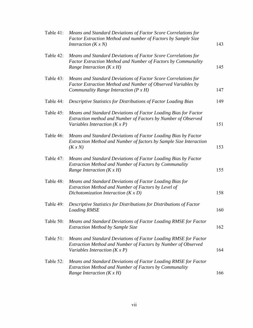
vii
Table 41: Means and Standard Deviations of Factor Score Correlations for Factor Extraction Method and number of Factors by Sample Size Interaction (K x N) 143
Table 42: Means and Standard Deviations of Factor Score Correlations for
Factor Extraction Method and Number of Factors by Communality Range Interaction (K x H) 145
Table 43: Means and Standard Deviations of Factor Score Correlations for Factor Extraction Method and Number of Observed Variables by Communality Range Interaction (P x H) 147 Table 44: Descriptive Statistics for Distributions of Factor Loading Bias 149 Table 45: Means and Standard Deviations of Factor Loading Bias for Factor Extraction method and Number of Factors by Number of Observed Variables Interaction (K x P) 151 Table 46: Means and Standard Deviations of Factor Loading Bias by Factor Extraction Method and Number of factors by Sample Size Interaction (K x N) 153 Table 47: Means and Standard Deviations of Factor Loading Bias by Factor Extraction Method and Number of Factors by Communality Range Interaction (K x H) 155 Table 48: Means and Standard Deviations of Factor Loading Bias for
Extraction Method and Number of Factors by Level of Dichotomization Interaction (K x D) 158
Table 49: Descriptive Statistics for Distributions for Distributions of Factor Loading RMSE 160 Table 50: Means and Standard Deviations of Factor Loading RMSE for Factor Extraction Method by Sample Size 162 Table 51: Means and Standard Deviations of Factor Loading RMSE for Factor Extraction Method and Number of Factors by Number of Observed Variables Interaction (K x P) 164 Table 52: Means and Standard Deviations of Factor Loading RMSE for Factor Extraction Method and Number of Factors by Communality Range Interaction (K x H) 166
viii
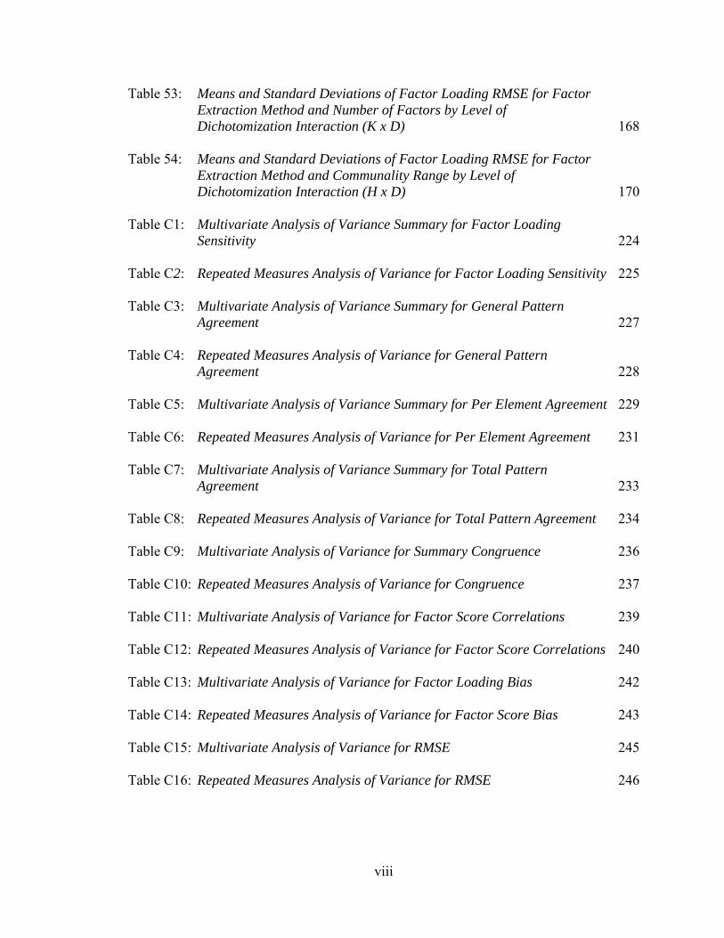
Table 53: Means and Standard Deviations of Factor Loading RMSE for Factor Extraction Method and Number of Factors by Level of Dichotomization Interaction (K x D) 168 Table 54: Means and Standard Deviations of Factor Loading RMSE for Factor Extraction Method and Communality Range by Level of Dichotomization Interaction (H x D) 170 Table C1: Multivariate Analysis of Variance Summary for Factor Loading Sensitivity 224
Table C2: Repeated Measures Analysis of Variance for Factor Loading Sensitivity 225
Table C3: Multivariate Analysis of Variance Summary for General Pattern Agreement 227
Table C4: Repeated Measures Analysis of Variance for General Pattern Agreement 228
Table C5: Multivariate Analysis of Variance Summary for Per Element Agreement 229
Table C6: Repeated Measures Analysis of Variance for Per Element Agreement 231
Table C7: Multivariate Analysis of Variance Summary for Total Pattern Agreement 233
Table C8: Repeated Measures Analysis of Variance for Total Pattern Agreement 234
Table C9: Multivariate Analysis of Variance for Summary Congruence 236
Table C10: Repeated Measures Analysis of Variance for Congruence 237
Table C11: Multivariate Analysis of Variance for Factor Score Correlations 239
Table C12: Repeated Measures Analysis of Variance for Factor Score Correlations 240
Table C13: Multivariate Analysis of Variance for Factor Loading Bias 242
Table C14: Repeated Measures Analysis of Variance for Factor Score Bias 243
Table C15: Multivariate Analysis of Variance for RMSE 245
Table C16: Repeated Measures Analysis of Variance for RMSE 246

List of Figures
ix
Figure 1. Flowchart summarizing the generation of population and sample matrices 58 Figure 2. Mean values of factor loading sensitivity by interactions between number of factors and observed variables 88 Figure 3. Mean values of factor loading sensitivity by interactions between number of factors and communality 91 Figure 4. Mean values of factor loading sensitivity by interactions between number of factors and level of dichotomization 93 Figure 5. Mean values of factor loading sensitivity by interactions between number of observed variables and communality 95 Figure 6. Mean values of general pattern agreement by interactions between number of factors and observed variables 101 Figure 7. Mean values of general pattern agreement by interactions between number of factors and communality 103 Figure 8. Mean values of general pattern agreement by interactions between number of observed variables and communality 106 Figure 9. Mean values of general pattern agreement by interactions between sample size and communality 108 Figure 10. Mean values of per element agreement by interactions between number of factors and number of observed variables 113 Figure 11. Mean values of per element agreement by interactions between number of factors and sample size 115 Figure 12. Mean values of per element agreement by interactions between number of factors and communality 117 Figure 13. Mean values of per element agreement by interactions between number of observed variables and communality 119
x
Figure 14. Mean values of per element agreement by interactions between sample Size and communality 122 Figure 15. Mean values of congruence by interactions between number of factors and number of observed variables 128 Figure 16. Mean values of congruence by interactions between number of
factors and sample size 130 Figure 17. Mean values of congruence by interactions between number of
factors and level of dichotomization 132 Figure 18. Mean values of congruence by interactions between sample size
and communality 134 Figure 19. Mean values of congruence by interactions between communality
and level of dichotomization 136 Figure 20. Mean values of factor score correlations by interactions between number of factors and number of observed variables 141 Figure 21. Mean values of factor score correlations by interactions between number of factors and sample size 144 Figure 22. Mean values of factor score correlations by interactions between number of factors and communality 146 Figure 23. Mean values of factor score correlations by interactions between number of observed and communality 148 Figure 24. Mean values of factor bias by interactions between number of
factors and number of observed variables 152 Figure 25. Mean values of factor bias by interactions between number of
factors and sample size 154 Figure 26. Mean values of factor bias by interactions between number of
factors and communality 156 Figure 27. Mean values of factor bias by interactions between number of
factors and level of dichotomization 159 Figure 28. Mean values factor loading RMSE by sample size main effect 163
xi
Figure 29. Mean values factor loading RMSE by interactions between number of factors and number of observed variables 165 Figure 30. Mean values factor loading RMSE by interactions between number
of factors and communality 167 Figure 31. Mean values factor loading RMSE by interactions between number of factors and level of dichotomization 169 Figure 32. Mean values factor loading RMSE by interactions between communality and level of dichotomization 171 Figure D1. Factor loading sensitivity by interactions between number of factors and observed variables 248 Figure D2. Factor loading sensitivity by interactions between number of factors and communality 249 Figure D3. Factor loading sensitivity by interactions between number of factors and level of dichotomization 250 Figure D4. Factor loading sensitivity by interactions between number of observed variables and communality 251 Figure D5. General pattern agreement by interactions between number of factors and observed variables 252 Figure D6. General pattern agreement by interactions between number of factors and communality 253
Figure D7. General pattern agreement by interactions between number of observed variables and communality 254 Figure D8. General pattern agreement by interactions between sample size and communality 255 Figure D9. Per element agreement by interactions between number of factors and number of observed variables 256 Figure D10. Per element agreement by interactions between number of factors and sample size 257 Figure D11. Per element agreement by interactions between number of factors and communality 258
xii
Figure D12. Per element agreement by interactions between number of observed variables and communality 259 Figure D13. Per element agreement by interactions between sample size and communality 260 Figure D14. Total pattern agreement by interactions between number of factors and observed variables 261 Figure D15. Total pattern agreement by interactions between number of factors and sample size 262 Figure D16. Total pattern agreement by interactions between number of observed variables and sample size 263 Figure D17. Mean values of congruence by interactions between number of factors and number of observed variables 264 Figure D18. Mean values of congruence by interactions between number of factors and sample size 265 Figure D19. Mean values of congruence by interactions between number of factors and level of dichotomization 266 Figure D20. Mean values of congruence by interactions between sample size and communality 267 Figure D21. Mean values of congruence by interactions between communality and level of dichotomization 268 Figure D22. Factor score correlations by interactions between number of factors and number of observed variables 269 Figure D23. Factor score correlations by interactions between number of factors and sample size 270 Figure D24. Factor score correlations by interactions between number of factors and communality 271 Figure D25. Factor bias by interactions between number of factors and number of observed variables 272 Figure D26. Factor bias by interactions between number of factors and sample size 273

xiii
Figure D27. Factor bias by interactions between number of factors and communality 274 Figure D28. Factor bias by interactions between number of factors and level of dichotomization 275 Figure D29. RMSE by interactions between number of factors and number of observed variables 276 Figure D30. RMSE by interactions between number of factors and communality 277 Figure D31. RMSE by interactions between number of factors and level of dichotomization 278 Figure D32. RMSE by interactions between communality and level of dichotomization 279

Abstract
xiv
This study is intended to provide researchers with empirically derived guidelines
for conducting factor analytic studies in research contexts that include dichotomous and
continuous levels of measurement. This study is based on the hypotheses that ordinary
least squares (OLS) factor analysis will yield more accurate parameter estimates than
maximum likelihood (ML) and principal axis factor anlaysis (PAF); the level of
improvement in estimates will be related to the proportion of observed variables that are
dichotomized and the strength of communalities within the data sets.
To achieve this study’s objective, maximum likelihood, ordinary least squares,
and principal axis factor extraction models were subjected to various research contexts.
A Monte Carlo method was used to simulate data under 540 different conditions;
specifically, this study is a four (sample size) by three (number of variables) by three
(initial communality levels) by three (number of common factors) by five (ratios of
categorical to continuous variables) design. Factor loading matrices derived through the
tested factor extraction methods were evaluated through four measures of factor pattern
agreement and three measures of congruence.

xv
To varying degrees, all of the design factors, as main effects, yielded significant
differences in measures of factor loading sensitivity, agreement between sample and
population, and congruence. However, in all cases, the main effects were components of
interactions that yielded differences in values of these measures that were at least
medium in effect size. The number of factors imbedded in the population was a
component in six interactions that resulted in medium effect size differences in measures
of agreement between population and sample factor loading matrices. of factor loading
sensitivity, general pattern agreement, per element agreement, congruence, factor score
correlations, and factor loading bias; in terms of the number of interactions that yielded at
least medium effect size differences in measures of sensitivity, agreement, and
congruence. The number of factors design factor exerted a larger influence than any of
the other design factors. The level of communality interacted with the number of factors,
number of observed variables, and sample size main effects to yield at least medium
effect size differences in factor loading sensitivity, general pattern agreement, per
element agreement, congruence, factor score correlations, factor loading bias, and RMSE;
in terms of the number of factors that included communality as a component, this design
factor exerted the second largest amount of influence on the measures of sensitivity,
agreement, and congruence. The level of dichotomization, sample size, and number of
observed variables were included in smaller numbers of interactions; however, these
interactions yielded differences in all of the outcome variables that were at least medium
in effect size.

xvi
Across the majority of interactions among the manipulated research contexts, the
ordinary least squares factor extraction method yielded factor loading matrices that were
in better agreement with the population than either the maximum likelihood or the
principal axis methods. In three of the four measures of congruence, the ordinary least
squares method yielded factor loading matrices that exhibited less bias and error than the
other two tested factor extraction methods. In general, the ordinary least squares method
yielded factor loading matrices that correlated more strongly with the population than
either of the other two tested methods.
The suggested use of ordinary least squares factor analytic techniques represents
the major, empirically derived recommendation derived from the results of this study. In
all tested conditions, the ordinary least squares factor extraction method identified
common factors with a high degree of efficacy. Suggested studies for future would
incorporate the limiting constraints associated with this dissertation into methodological
studies to extend the generalizability of conclusions and recommendations into areas that
are beyond the scope of this dissertation.

Chapter One
1
Introduction
The existence of internal attributes, or factors, is the central assertion in factor
analytic theory (Tucker & MacCallum, 1997). While these factors are not directly
observable, much of the variation in the phenomena that researchers witness and measure
is attributable to these underlying traits (Bartholomew, 1984; Cureton & D’Agostino,
1983; Stevens, 2002; Tucker & MacCallum, 1997). Moreover, factor analytic theory
asserts that these hypothetical, internal attributes are more “fundamental” than the surface
attributes which we observe (Tucker & MacCallum, 1997, p. 2).
In the most basic sense, factor analysis is a set of procedures that researchers
employ to analyze relationships among variables (Cureton & D’Agostino, 1983). The
objective of this set of procedures is to account for complex patterns of covariation
among observed random variables with a set of common factors. The central goals of
exploratory factor analysis include the identification of theoretical constructs that
underlie a set of observations and the quantification of the extent to which these
constructs “represent the original variables” (Henson & Roberts, 2006, p. 396).
The method through which factors are extracted from data represents one of the
central procedures associated with exploratory factor analysis (Cureton & D’Agostino,
1983; Stevens, 2002; Tucker & MacCallum, 1997). The goal of this study is to provide
researchers with empirical data regarding the most common methods of factor extraction;
2
the result of this study will be a performance assessment of specific factor extraction
techniques applied to a variety of research conditions. To simulate many samples within
a large spectrum of research contexts, this study will employ a Monte Carlo simulation
(Metropolis & Ulam, 1949).
Statement of Problem
Although exploratory factor analysis is useful in “both measurement and
substantive research contexts” (Henson & Roberts, 2006, p. 396), it has been subjected to
persistent criticism. Many of these objections are based on the subjectivity of the
decisions that researchers must make when conducting their factor analyses (Henson &
Roberts, 2006). Another important source of criticism is related to the “indeterminacy of
factor solutions” (Harman, 1976, p. 27) which implies that, for a given matrix of
correlations, an infinite number of uncorrelated factors can be selected.
Attempts to incorporate non-normal data types into factor analyses represent
another potential area of criticism (Yuan, Marshall, & Bentler, 2002). Guiding principles
are well established for contexts that include continuous variables that exhibit
multivariate normality. However, “no firm guidelines have as yet emerged concerning
situations in qualitative and quantitative variables are mixed together” (Krzanowski,
1983, p. 235).
The lack of guidelines associated with incorporating non-normal data sets into
factor analytic studies represents the problem to be addressed by this dissertation. The
absence of these guidelines becomes especially salient as researchers attempt to
incorporate mixtures of continuous and categorical data into factor analytic studies.
Without empirically derived guidelines for conducting factor analytic studies with these

3
types of complex data sets, factor analytic design choices can be criticized as subjective
which yield results that can be considered problematic.
Theoretical Framework
While the work of Pearson represents the mathematical foundation for classical
factor analysis, Spearman provided the initial description of statistical treatments
associated with principal axis analyses (Harman, 1976). Spearman’s (1904) work in
identifying the strength and direction of relationships among intellectual abilities
describes a method for extracting “something of substance” (Spearman, 1904, p. 258)
from correlations. This study of intelligence and its advocacy for the use correlation
studies in the field of psychology serve as the theoretical basis for this dissertation.
In a series of four experiments, Spearman collected demographic and
performance data from 123 students. These subjects were sampled from both a set of
village schools and a preparatory academy. In terms of chronological age, students from
the preparatory academy were drawn from the highest class. Students from the village
schools were selected based on their relative position with respect to age; these students
were the oldest children in their families (Spearman, 1904).
After gathering information regarding height, weight, and age, Spearman
subjected the students to a variety of perceptual acuity, or discernment, tests. Spearman
also assessed the students’ performance in a variety of academic skills which included
Latin, Mathematics, French, English, Music, and Greek. To examine each student’s
outward expression of common sense and general intelligence, Spearman included
interviews of the test subjects’ classmates, siblings, and teachers.

4
Spearman’s initial discussion regarding the experimental results focused on
defining the method through which true correlations could be derived from observed
correlations (Spearman, 1904). The development of this true correlation required the
following four steps:
1. Determine the strength of the observed correlations.
2. Estimate the amount of errors included in correlations between two sets of
variables.
3. Identify any spurious correlations or “any factors irrelevantly admitted”
(Spearman, 1904, p. 257).
4. Critically examine the experimental design and theory supporting the design to
identify any disturbing factors.
Based on the observed correlations, Spearman attempted to measure the extent to which
two series of observations had something of substance in common. The existence of this
common substance is asserted when the observed correlation is at least four to five times
greater than the amount of error associated with the estimate (Spearman, 1904).
The study yielded a hierarchy of intelligences that Spearman summarized through
a table of correlations among observed variables. This matrix contained corrected
correlations which represent estimates of association after observational errors were
eliminated (Spearman, 1904); the main diagonal of this matrix contained values less than
one. This hierarchy of intelligences is presented through a table containing correlations
between sensory discernment and school subject performance observations, a factor of
general intelligence, and a column presenting ratios of the common factor to specific
factors (Spearman, 1904).

5
Spearman concluded that all branches of intellectual capacity had in common
“one fundamental function” (Spearman, 1904, p. 284). The remaining elements of
intellectual activity are unique for each observation. Spearman’s description of
observations in terms of common and specific factors represents a fundamental premise
in common or classic factor analytic theory.
The common factor to which Spearman referred is an unobservable, internal
attribute that influences the value of observed variables (Tucker & MacCallum, 1997).
These hypothetical constructs, in conjunction with researchers’ theories, can be used to
explain “the variation and covariation across a wide range of surface attributes” (Tucker
& MacCallum, 1997, pp. 2-3). Factor analytic theory includes two types of internal
attributes; these are common factors and specific factors.
Formally, a common factor is “an internal attribute which affects more than one
of the surface attributes in the selected set, or battery” (Tucker & MacCallum, 1997, pp.
2-3). While still being an internal attribute, a specific factor influences only one variable
in a given data set. A third type of influence includes measurement error; this influence
is neither internal nor systematic (Tucker & MacCallum, 1997).
The “traditional” or “classical” factor analysis model is defined by the following
equation:
⋯ 1, 2,⋯ ,
In this model, a variable is described by a linear combination of common factors
, , ⋯ , , and a unique factor . The a’s represent coefficients or loadings for
the common factors; the number of common factors (m) is normally smaller than the

6
number of observed variables, n (Harman, 1976). When considering the value of a
specific variable, j, for a given individual, i, the factor model can be written as:
Where is the common factor p for individual i; represents the contribution of
the factor on the linear composite. The residual error is given by (Harman, 1976).
The factor analytic model provides estimates for the values of loadings on
common factors (Harman, 1976). Classical factor analysis includes many strategies for
extracting these factor loadings from data. The manner in which researchers select
specific methods for factor extraction represents the focus of this study.
Recent developments in structural equation modeling define formative factors as a
category of latent variables that are neither common nor unique. As opposed to factor
analytic theory, in which observed variables are attributable to factors, formative factors
are generated by observed variables (Bollen & Lennox, 1991; Kim, Shin, & Grover,
2010; Treiblmaier, Bentler, & Mair, 2011). In formative measurement models, indicators
cause latent variables in the following manner (Bollen & Lennox, 1991):
⋯
In this expression, γ’s are coefficients, χ’s are “explanatory or observed variables”
(Bollen & Lennox, 1991, p. 306), and the dependent variable is the latent construct, .
In the field of information sciences, recent reviews of literature highlight the
increased importance of structural equation modeling and the use of formative
measurement models (Kim, Shin, and Grover, 2010). For example, searches of MIS
Quarterly and Information Systems Research, yielded 24 articles published since 2001
7
that focused on formative latent variables. In addition to noting the prevalence of
formative constructs in the published literature, Kim, Shin, and Grover (2010) examined
the differing perspectives regarding the utility of formative latent variables, design issues
associated formative measurement models, and the impact of these models on the
“quality of IS research . . .” (Kim, Shin, & Grover, 2010, p. 363). They identified
“interpretational confounding” and “external consistency” as central issues in the
controversy among information scientists over the “viability of formative indicators”
(Kim, Shin, & Grover, 2010, p. 347).
Interpretational confounding occurs when empirical meaning is assigned to an
unobserved variable in a manner that does not agree with the a priori meaning given to
the variable by the researcher (Kim, Shin, & Grover, 2010). Researchers who oppose the
use of formative constructs cite the requirement of additional endogenous variables to
estimate “formative indicator weights” (Kim, Shin, & Grover, 2010, p. 347) as a major
factor contributing the prevalence of interpretational confounding in formative
measurement models. Moreover, the few solutions to these identification problems
include the expansion of formative measurement models to include reflective indicators
(Kim, Shin, & Grover, 2010; Treiblmaier, Bentler, & Mair, 2011).
External consistency is achieved “when the measures of a construct correlate with
the measures of other constructs” (Kim, Shin, & Grover, 2010, p. 347). Unlike reflective
measurement models, the constructs associated with formative models do not maintain
linkages with “antecedents and consequences of a construct” (Kim, Shin, & Grover,
2010, p. 347). Proponents of formative measurement models assert that external

8
consistency and interpretational confounding are not salient issues when models are
correctly specified (Kim, Shin, & Grover, 2010).
To examine the relative strengths of these competing perspectives concerning
formative measurement models and their associated constructs, Kim, Shin, and Grover
(2010) studied an existing dataset derived from an information technology survey. The
survey included 243 respondents and two exogenous variables. These two variables
include: “IT infrastructure flexibility as formatively theorized construct” and “relational
knowledge as a reflectively theorized construct” (Kim, Shin, & Grover, 2010, p. 350).
The constructs were measured via index and conventional scale development procedures
(Kim, Shin, & Grover, 2010). The endogenous variables included financial performance,
information technology performance, business process performance, effectiveness in
information technology planning, and effectiveness in information technology
coordination. The variables were analyzed through both correctly and incorrectly
specified models (Kim, Shin, & Grover, 2010).
The researchers’ results indicated that formative measurement models posed
“fundamental problems” in estimating weights (Kim, Shin, & Grover, 2010, p. 359).
They found substantial interpretational confounding; moreover, the lack of external
consistency leads to “unpredictability of model fit . . ..” (Kim, Shin, & Grover, 2010, p.
363). Ultimately the researchers concluded that the use of formative measure models has
substantial and negative impact on the quality of information systems research (Kim,
Shin, & Grover, 2010).
Researchers concede that, under limited conditions, a formative construct may
be scientifically meaningful. However, these same researchers assert that a thoughtfully

9
developed reflective measurement approach is the most practical (Treiblmaier, Bentler,
& Mair, 2011). The reflective (common factor) approach to construct development is
the focus of this dissertation.
Purpose of the Study
Objective. This study is intended to provide researchers with empirically derived
guidelines for conducting factor analytic studies in complex research contexts.
Specifically, the scope of this study includes the evaluation of factor extraction methods
when applied to data sets that contain mixtures of categorical and continuous variables.
To enhance the potential utility of this study, the research focused on factor extraction
methods commonly employed by social scientists; these methods include principal axis
factor analysis, ordinary least squares factoring, and standard maximum likelihood
method.
To meet the goal of this study, factor extraction models were subjected to several
research conditions. These contexts differed in sample sizes, number of variables,
communalities, number of common factors, and ratios of categorical to continuous
variables. Data were simulated under 540 different conditions; specifically, this study
employed a four (sample size) by three (number of variables) by three (initial
communality levels) by three (number of common factors) by five (ratios of categorical
to continuous variables) design.
Rationale. One measure of the prevalence of factor analytic research designs in
contemporary literature can be found in a recent analysis of literature published in
PsycInfo over a two-year period. By focusing on this published research, the survey
yielded more than 1700 articles that involved exploratory factor analytic research

10
(Costello & Osborne, 2005). The variety of purposes to which these factor analyses are
applied also highlights the importance of this statistical tool. As Conway and Huffcutt
noted (2003), social scientists employ exploratory factor analysis to refine measurement
tools, establish construct validity, and test hypotheses. The proliferation of exploratory
factor analysis in social science research has served as justification for a number of
studies that either attempt to establish research design guidelines or contrast typical
practices with ideal reporting procedures (Costello & Osborne, 2005; Henson & Roberts,
2006; Krzanowski, 1983).
Although exploratory factor analysis is useful in “both measurement and
substantive research contexts (Henson & Roberts, 2006, p. 396),” it has been the focus of
methodological criticism. According to Henson and Roberts (2006), many of the
objections to the use of exploratory factor analysis are based on the “inherent subjectivity
of the decisions” ( p. 396) that researchers must make when conducting their analyses.
For example, without referring to criterion variables, researchers select matrices of
association, factor extraction methods, criteria for retaining factors, factor rotation
strategies, and coefficients for interpretation (Henson & Roberts, 2006).
As social scientists attempt to incorporate data sets that contain diverse
preference, socio-economic, and quality of life measures into their multivariate analyses,
they cannot rely on empirically developed guidelines. While these types of guidelines are
well established for contexts that include continuous variables that exhibit multivariate
normality, they are not as useful when applied to contexts that include mixtures of
qualitative and quantitative data (Krzanowski, 1983). This difficulty in applying
exploratory factor analysis becomes especially pronounced when the research context

11
includes categorical variables (Krzanowski, 1983). The lack of methodological
guidelines contributes to the rationale for this study.
Supporting Examples.
First supporting example. To identify the factor structure of risky sexual
behavior and substance use, the Vanzile-Tamsen, Testa, Harlow, and Livingston (2006)
recruited 1,014 college women to participate in a study of sexual risk taking behavior.
The levels and types of risk taking behavior, alcohol use, and drug use were assessed via
a “computer assisted self interview” (VanZile-Tamsen et al. 2006, p. 250). As part of
the study’s design, the researchers included observed variables from two domains: Sexual
risk taking and Substance Use (VanZile-Tamsen et al., 2006).
The sexual risk taking behaviors include eight variables measured at a variety of
levels. The authors assessed age at first sexual encounter as a ratio level measure. A
subject’s number of life time partners was measured at an interval level; this included
seven levels that ranged from 0 to 10 or more (VanZile-Tamsen et al., 2006). The time
between meeting a new partner and having sex with him is measured through a six-level,
Likert-type scale; a score of one indicates the first day that a subject meets a new partner,
and a score of six means a year or more after meeting a new partner.
Also as part of the sexual risk taking domain, the researchers developed a
complex indicator of alcohol use associated with sexual encounters; this continuous
indicator represents composite of two, Likert-type variables. The first part of the index
measured the number of times that alcohol use occurred prior to or during intercourse;
this measure had five levels ranging from 1 (once in a while) to 5 (all the time). The
second part of this index measured the level of intoxication during sex; this Likert-type

12
response scale ranged from 1 (not at all intoxicated) to 7 (very intoxicated). Neither
portion of this composite variable defined the distances between the levels as equivalent.
Without this information, the variables could (at most) be considered ordinal.
The last set of variables associated with sexual risk taking involved the perception
of sexually transmitted infection (STI) risk of each partner. This variable is an index
based on the subject’s estimate of life-time sexual partners that a new partner had and the
subject’s belief that a new partner has had sex with men, ever had or transmitted an STI,
and ever injected drugs (Vanzile-Tamsen et al., 2006).
Substance use was measured via four variables. The number of drinks during a
typical drinking occasion is measured at the ratio level. Frequency of binge drinking was
measured on a 6 point Likert-type scale. Frequency of drinking occasions contains a
Likert-type response set with eight levels. A drug use index was derived from the
number of illicit drugs used, the frequency of drug use (a Likert-type response scale), and
the results of a drug abuse screening test.
Impulsivity, sensation seeking, and anxiety were measured through 38 yes/no
items. These dichotomously scored items were all highly correlated and used to construct
three latent variables that would be included in a more general model. Negative affect
consisted of counts of 10 depressive symptoms and 21 trauma symptoms from the DSM
IV.
The researchers employed a maximum likelihood confirmatory factor analysis to
compare three models of risk behavior. The comparisons were based on three fit indices,
root mean squared error of approximation (RMSEA), and a “chi-squared difference test”
(Vanzile-Tamsen et al., 2006, p. 250). Based on the results of these comparisons, the

13
authors proposed a four latent factor model to account for their observations; this model
contained two higher order factors (Vanzile-Tamsen et al., 2006).
The researchers highlighted several limitations associated with their study. For
example, the model includes direct influences from personality factors to risk-taking
behaviors; however, these influences “represent partial correlations . . .” (Vanzile-
Tamsen et al., 2006, p. 253). Due to the researchers’ efforts to identify a model that best
fit their data, “no conclusions should be made with regards to the model’s usefulness
outside of community samples” (Vanzile-Tamsen et al., 2006, p. 2006). The researchers
attributed the complexity of their accepted factor model to the use of multiple indicators
for each domain.
Second supporting example. To improve the quality of evaluative research in
civics education, Finkel and Ernst (2005) presented the findings of a study conducted in
1998. This study examined the “impact of civic education” (Finkel & Ernst, 2005, p.
335) on South African high school students. The sample included 600 students; 385 of
these students were exposed to formal civics education, and 261 of whom participated in
this education through the U.S. Agency for International Development (USAID)
“Democracy for All” (Finkel & Ernst, 2005, p. 335) program. The remaining 215
students did not receive formal civics education.
The researchers used a battery of items to determine students’ “political
knowledge, civic duty, tolerance, institutional trust, civic skills, and approval of legal
forms of political participation” (Finkel & Ernst, 2005, p. 335). Binary response and
correct/incorrect items were used to assess knowledge. Items measured on a Likert-type
scale were used to assess indices of civic duty, political tolerance, trust in political

14
institutions, and approval of political participation, and interval level measures were used
to assess students’ perceptions of their own civic skills (Finkel & Ernst, 2005).
Civic education was assessed through measures of “students perceptions of
teacher quality” (Finkel & Ernst, 2005, p. 347), frequency of exposure to civic education,
and teaching methods. Frequency of education was measured through a single Likert-
type item, ratio scale index scores were used to measure perceptions of teacher quality.
Binary items were used to obtain information concerning active teaching methods (Finkel
& Ernst, 2005).
In total, this study included 53 observed variables. Of these, 25 items were
measured on a binary scale (either yes/no or correct/incorrect); four items were measured
on an ordinal scale, and 24 items were measured at the interval level. The items measured
at the interval level included 19 variables which yielded Likert-type observations. The
researchers presented their results through a table containing two sets of factor loading
coefficients; one set of coefficients were associated with students who received civics
education, and another set was associated with students who received no civics education.
Through comparing the strengths of loading coefficients, the researchers highlighted
slight differences in loadings between the groups. The results of this study did not yield a
comprehensive model of political engagement that could be subjected to a confirmatory
analysis.
Through empirically derived guidelines for incorporating differing scales of
measurement into a single exploratory factor analysis, the authors would have been in a
better position to incorporate all of their observations into a single, parsimonious factor
model. This model would have demonstrated the manner in which demographic

15
variables and instructional characteristics interact with behavioral outcomes to yield a
comprehensive model of political engagement. Such an analysis would be more
amenable to replication and more easily subjected to confirmatory analysis.
Research Questions
The agreement between factor pattern matrices in a simulated population and
matrices developed through selected exploratory factor analytic techniques is the primary
comparison associated with this study. This agreement was assessed through the
proportion of variables that load on the same factors, total factor loading agreement, and
factor loading congruence coefficients (MacCallum et al., 1999). Measures of
agreement, correlations between population and sample factor score matrices, root mean
square error, statistical bias, and solution variability were considered as measures of
factor pattern agreement.
The measures of congruence and agreement among population and sample
matrices were used to answer the following research questions:
1. How do varying ratios of categorical to continuous variables influence the
agreement between factor pattern matrices extracted through the examined factor
analysis strategies and factor pattern matrices simulated in the population?
2. How does the number of variables in a correlation matrix influence the agreement
between factor pattern matrices extracted through the examined factor analysis
strategies and factor pattern matrices simulated in the population?
3. How does sample size influence the agreement between factor pattern matrices
extracted through the examined factor analysis strategies and factor pattern
matrices simulated in the population?

16
4. How does communality influence the agreement between factor pattern matrices
extracted through the examined factor analysis strategies and factor pattern
matrices simulated in the population?
5. How does the number of common factors influence the agreement between factor
pattern matrices extracted through the examined factor analysis strategies and
factor pattern matrices simulated in the population?
6. How do all of the independent variables interact to influence the agreement
between factor pattern matrices extracted through the examined factor analysis
strategies and factor pattern matrices simulated in the population?
Hypotheses
This study focused on comparisons among three factor extraction methods; these
methods include principal axis factor analysis, ordinary least squares factor analysis, and
maximum likelihood factor analysis. Each factor extraction method was subjected to the
same variety of research conditions. The hypotheses associated with this study were
evaluated through the measures defined in the research questions.
First hypothesis. The first hypothesis asserted that ordinary least squares (OLS)
factor analysis will perform better than maximum likelihood factor analysis as the
number of dichotomously scored variables increases. Research into factor analytic
techniques indicate that iterative, principal axis factor extraction methods perform better
than maximum likelihood methods when the assumption of multivariate normality is not
met (Bartholomew, 1980). Based on the findings of earlier research, this study also
asserts that, when the research context includes dichotomously scored variables,
17
maximum likelihood factor analysis will yield factor structures that are less like those
simulated in the population than principal axis factor analysis.
Second hypothesis. The second hypothesis asserted that, when the factor structure in
the population is not strongly defined, ordinary least squares (OLS) factor analysis will
identify common factors that maximum likelihood factor analytic methods fail to
identify. According to this hypothesis, OLS’s relative advantage in identifying common
factors will be negatively related to communality and positively related to the number of
dichotomous variables. This hypothesis is based on two complimentary studies that
highlight OLS’s insensitivity to error and maximum likelihood’s reliance on the
assumption of multivariate normality (Briggs & MacCallum, 2003; Mislevy, 1986).
Significance of the Study
As a tool for generating theory, exploratory factor analysis can play a vital role in
developing a knowledge base for social scientists (Stevens, 2002). However, the quality
of this knowledge base will be directly related to the quality of the decisions that
researchers make as they implement their factor analysis procedures (Bartholomew,
1984; Henson & Roberts, 2006; Tucker & MacCallum, 1997). As one of the primary
decisions that a researcher must make, the selection of a factor extraction strategy has a
tremendous impact on the quality of conclusions derived from an exploratory factor
analytic design. This study can provide researchers with useful guidance in this selection
process.
Several recent studies have proposed a variety of Bayesian latent trait models to
be employed by researchers when they encounter discrete and mixed data research
contexts (Merkle, 2005; Sammel, Ryan, & Legler, 1997; Song & Lee, 2001). However,

18
these types of exploratory factor analysis strategies are not often used by social science
researchers (Henson & Roberts, 2006). Because this study included principal axis,
maximum likelihood, and ordinary least squares factor extraction techniques, the results
can provide researchers with empirical information concerning the factor extraction
methods that they are likely to use.
Definition of Terms
Categorical Level of Data--or nominal data is the result of assigning
numbers to categories; this is the “most rudimentary” level of measurement in which all
individuals assigned to a given group are the same in terms of a characteristic or set of
characteristic (Glass & Hopkins, 1996, p. 7).
Congruence - among factor pattern matrices simulated in the population and the
sample pattern matrices is measured through a congruence coefficient. As defined by
MaCallum (et al., 1999), the phi coefficient is the cosine of the angle between the sample
and population factor solutions “when plotted on the same space” (p. 93). To assess the
congruence across all factor loading matrices, an average of the phi coefficient was
calculated for each factor extraction method.
Continuous Level Data--consist of measures that can be any value within a
specified range (Glass & Hopkins, 1996).
Factor Loadings--are the coefficients of the factors in the basic factor model. The
ambiguous use of the term is problematic when the factors are correlated. To interpret
the resulting factor solutions, correlated factor solutions undergo oblique rotations and
yield two distinct factor matrices: factor pattern and factor structure (Harman, 1976).

19
Factor Loading Bias – is one measure of a factor extraction methods performance;
it is a number of observed variables by number of factors matrix which is populated by
estimates of statistical bias for each factor loading; in this study these bias estimates were
averaged across all samples (Hogarty et al., 2005).
Factor Loading Root Mean Squared Error – is an indicator of congruence between
sample and population factor loading matrices. This outcome variable is a number of
observed variables by number of factors matrix containing root mean squared error
(RMSE) estimates for each factor loading To provide an overall index for each factor
solution, the RMSE estimates are averaged across all samples in each research context
(Hogarty et al., 2005).
Factor Loading Sensitivity- is one of the measures of agreement between sample
and population factor loading matrices. This is the count of variables that meet a .30
factor loading threshold for at least one factor in both the sample and the population
divided by the count of variables that meet the .30 loading threshold in the population
(Hogarty et al., 2005).
Factor Score Correlations - is a number of factors by 1 column vector of
correlations between factor scores derived from the sample and those derived from the
population. These score estimates will be linear combinations of variables; however, as
opposed to using factor score coefficients, these estimates will be computed via the
following process: A positive one scoring coefficient is assigned when the observed
structure coefficient is .30; a negative one scoring coefficient is assigned when the
observed structure coefficient is .30; a scoring coefficient of zero is assigned when
the structure coefficient is between .30 and -.30. Once factor scores estimates are
20
computed for both the population and sample matrices, a correlation among the scores
will be used to measure how closely factor scores derived from each of the factor
extraction strategies approximates that factor score pattern that is imbedded in the
population (Hogarty et al., 2005).
General Pattern Agreement-- is one of the measures of agreement between sample
and population factor loading matrices. This variable is based on the proportion of
variables that load on both the sample and population factors in a similar fashion at least
once. This variable is a number of observed variables by one column vector. When the
absolute value of the variable loading on the same factor in boht the sample and the
population is greater than or equal to .30, then a one is assigned to the row associated
with the variable. For this measure a variable can meet this threshold for multiple factors
and still contribute to general pattern agreement (Hogarty et al., 2005).
Monte Carlo Experiments--refer to a class of experiments in which researchers
employ computer programs to generate “vectors of random variates” that are analogous
to samples of data (Robey, 1990, p. 278). These samples are derived from a population
model containing characteristics of interest to the researcher. Monte Carlo simulations
can be used to demonstrate the influence that a variety of research contexts can have on
an experiment (Robey, 1990).
Per Element Agreement – is based on a number of observed variables by number
of factors matrix. Elements of each matrix contain ones, indicating agreement, where the
corresponding factor loading has an absolute value of .30 or greater in both the sample
and population factor pattern matrices; elements of the matrix also contained ones when
the absolute value of the loading for a variable was less than.30 in both the sample and

21
the population. When these criteria are not met, the element is assigned a zero. The
resulting outcome measure is the proportion of samples in which the agreement criteria
were met for each observed variable by factor combination (Hogarty et al., 2005).
Total Pattern Agreement - is measured through a scalar. This scalar is populated
with a one when the mean of the per element agreement matrix is one. If any element of
the per element agreement matrix is less than one, then the mean of that matrix will be
less than one, and the total pattern agreement scalar associated with that matrix is set to
zero. This scalar represents the proportion of sample matrices in which all factor
loadings are in agreement with the population in terms of the absolute value of .30
loading criterion (Hogarty et al., 2005).
Delimitations
The objective of this study was to provide researchers with empirically derived
guidelines for conducting factor analytic studies in complex research contexts.
Specifically, the scope of this study included the evaluation of factor extraction methods
when applied to data sets containing mixtures of categorical and continuous variables.
The extent to which the results of this study can be generalized is limited by certain
characteristics associated with the simulation of sample data and the selection of factor
analytic studies that are the focus of this dissertation.
The correlation matrices through which data were simulated were be based on
factor models in which the influences of minor factors are constrained to zero. These
factor models were included uncorrelated factors exclusively. When extracting factors
from sample data, the number of factors to be retained was equal to the number of factors
simulated in the population. In addition to these research design decisions, the selection
22
of only three commonly employed factor analytic strategies imposed a limit to which the
potential guidelines derived from this study can be generalized.
Organization of Remaining Chapters
The next chapters include a review of literature and a description of the methods
through which the research questions were addressed. Chapter two contains a general
review of methodological research associated with exploratory factor analytic techniques
and a more focused analysis of the three factor extraction methods that represent the
primary focus of this study. Chapter three describes the manner in which correlation
matrices were generated, the method for simulating specific research conditions,
measures employed to compare sample and population factor patterns, and measures by
which factor extraction strategies were evaluated.
Chapters four and five present the results of the study and a discussion of the
results. Chapter four provides results divided into specific sections associated with each
outcome variable; the chapter includes a summary of results, and responses to each of the
research questions. Chapter five begins with a restatement of the study’s purpose, its
research questions, and a summary of the research methods. In addition to a general
discussion of results, chapter five includes a discussion of the results in terms of each
hypothesis and its applications to follow-up studies.

Chapter Two
23
Literature Review
The sequence of decisions that researchers make when designing and
implementing an exploratory factor analytic study provides this dissertation with a three-
part structure around which the literature review was organized. The first section of this
literature review extends the theoretical framework to include a general examination of
the design choices associated with factor analytic research. This overview includes
model selection, samples of subjects, samples of variables, multivariate normality, data
types, matrices of association, factor retention, and rotation strategies. The second
section of this review focuses on descriptive literature regarding principal axis factoring,
ordinary least squares factor extraction, and maximum likelihood factor analysis;
technical descriptions of these factor analytic methods are provided in Appendix A. The
last section of this literature review summarizes several simulation studies conducted on
various aspects of factor analysis.
Exploratory Factor Analysis Design Considerations
Model selection. In general, social science researchers employ factor analysis to
pursue three objectives: data reduction, identification of influences on overt behavior, and
confirmation of hypotheses regarding influences on behavior (Cureton & D’Agostino,
1983; Merrifield, 1974; Stevens, 2002). When the researcher’s intent is data reduction
only, then exploratory or common factor analysis is not the appropriate design; in this
24
case, the researcher should conduct a principal component analysis (Conway & Huffcutt,
2003; Fabrigar, MacCallum, Wegener, & Strahan, 1999, p. 273; Henson & Roberts,
2006; Merrifield, 1974; Stevens, 2002). When a researcher is confirming an existing or
well understood structural or measurement model, then confirmatory factor analysis
would be a more appropriate design than exploratory factor analysis. If a researcher
believes that the relationships among observations can be accounted for by underlying
characteristics but is unsure of the number or the organization of these characteristics,
then the decision to conduct an exploratory factor analysis (EFA) is justifiable (Cureton
& D’Agostino, 1983; Harman, 1976; Stevens, 2002).
The interactions among researchers’ intentions and the state of knowledge in
given fields represent critical considerations in the design of an exploratory factor
analysis (Raykov & Marcoulides, 2006; Stevens, 2002). Exploratory factor analysis
provides researchers with information concerning the number of common factors and
matrices of factor loadings (Harman, 1976). In this context, exploratory factor analysis is
a useful set of tools for generating new theories or modifying existing ones (Cureton &
D’Agostino, 1983; Harman, 1976; Stevens, 2002).
Conway and Huffcutt (2003) examined the quality of factor analytic research
published between 1985 and 1999. Their study indicated that preliminary evaluations of
ad-hoc instruments represented the most prevalent purpose behind factor analytic
research; assessing the performance of existing measures represented the next most
commonly reported purpose. Testing unidimensionality represented one of the least
reported purposes (Conway & Huffcutt, 2003).

25
According to the Conway and Huffcutt (2003) study, principal components
analysis (PCA) was the most frequently cited method for analyzing data. When factor
analysis represented the “important goal” of the study, common factor analysis was more
frequently cited than PCA (Conway & Huffcutt, 2003, p. 160). However, in 28% of the
articles, researchers failed to describe either their intention behind their analyses or
methods for extracting factors (Conway & Huffcutt, 2003).
Henson and Roberts (2006) examined the information reported in 60 exploratory
factor analyses published before 1999. The authors focused on studies that employed at
least one exploratory factor analysis strategy. Although Henson and Roberts noted that
most of the articles reported researcher objectives that warranted an EFA design, nearly
57% of the researchers engaged in principal components analysis. As a suggested
rationale for this problematic model selection, the authors noted that principal
components analysis was the “default option for most statistical software packages”
(Henson & Roberts, 2006, p. 403).
Samples of subjects. In exploratory factor analysis, common prescriptions
regarding specific subject per measured variable ratios are simplistic and problematic
(Fabrigar et al., 1999). These types of guidelines fail to account for levels of over-
determination and communalities among measured variables. Moreover, if the sample is
more homogeneous on the common factors than the population, high sample to measured
variable ratios will not ameliorate the restriction of range in observations and the
resulting attenuation in the correlations among variables (Fabrigar et al., 1999).
When each factor is represented by three to four measured variables and the
communalities exceed .70, relatively small sample sizes will allow researchers to make

26
accurate estimates about population parameters (Fabrigar et al., 1999). If researchers
believe that a sample of convenience may be inappropriate, methodological studies
highlight a number of sampling strategies that can be employed. For example, to avoid
distortions derived from sample characteristics, researchers can select a sample that
maximizes variance on measured variables that are not relevant to the construct of
interest (Fabrigar et al., 1999).
Recent assessments of published factor analyses indicate that many researchers
either do not have sample sizes large enough to support their study designs or do not
provide sufficient information concerning sampling strategies. In Conway and Huffcutt’s
(2003) assessment of 371 articles published between 1985 and 1999, nearly half the
studies included sample sizes of 200 or less, and 40% of the studies had sample to
variable ratios of 10:1 or less (Conway & Huffcutt, 2003). In a similar study completed
in 2006, Henson and Roberts found that the median sample to variable ratio was 11:1;
they concluded that “most samples sizes were marginal to sufficient, depending on
component saturation” (Henson & Roberts, 2006, p. 402).
Samples of variables. The selection of variables represents another important
element in the set of decisions that comprise a factor analytic research design. When
researchers include too few variables, they may not have a sufficient sample of variables
from the domain to identify important common factors; however, by including many
irrelevant measured variables, researchers may include “spurious common factors” that
obscure the “true” factors (Fabrigar et al., 1999, p. 273). Although prescriptions
regarding the total number of variables required to conduct factor analysis are not
prevalent in the literature, methodological research highlights the positive relationship

27
between overdetermination and factor accuracy (Fabrigar et al., 1999; Guadagnoli &
Velicer, 1988; Hogarty et al., 2005). Moreover, methodological research suggests that as
the number of factors increases with respect to the number of measured variables, the
accuracy and reliability of factor solutions decreases (Guadagnoli & Velicer, 1988).
Because communality and over-determination exert a strong influence on the
quality of factor solutions, these facets of factor analytic research warrant reporting.
However, assessments of common research practices indicate that researchers fail to
describe their measured variables comprehensively (Conway & Huffcutt, 2003; Henson
& Roberts, 2006). For example, in their 2006 survey of factor analytic research, Henson
and Roberts found that fewer than 17% of the articles that they examined reported
communalities among measured variables.
Scale coarseness and dichotomization. A response scale is considered course
when a continuous trait is measured in such a way that a variety of “true scores are
collapsed into the same category” (Aguinis, Pierce, & Culpepper, 2009, p. 625). In
exploratory factor analysis, continuous constructs observed through Likert type responses
represent commonly encountered occurrences of scale coarseness (Aguinis, Pierce, &
Culpepper, 2009). Research into the effects of scale coarseness indicates that, in many
research contexts, scale coarseness leads to downward bias in correlations (Aguinis,
Pierce, & Culpepper, 2009).
Scale coarseness is an artifact of a study’s design; it is the result of the
measurement instrument (Aguinis, Pierce, & Culpepper, 2009). Because dichotomization
introduces error after data are collected, it does not contribute to scale coarseness
(Aguinis, Pierce, & Culpepper, 2009; Cohen, 1983). However, the downward bias that it
28
causes in correlation is “centrally a measurement issue;” because the loss of information
is systematic, the “dichotomization drop will occur for both true and observed scores”
(Cohen, 1983, p. 252).
Cohen identifies four common rationales used by researchers as they dichotomize
their data. First, they employ dichotomization to use loglinear models; this practice is
similar to dichotomizing on a control variable in analyses of variance designs (Cohen,
1983). Second, researchers will dichotomize a set of scaled items in preparation for a
factor analysis. This rationale for dichotomization is problematic for a number of
reasons; for example, the resulting phi coefficients and factor loadings are only two-
thirds as large as the product-moment correlations on the original data (Cohen, 1983).
Moreover, regardless of estimation method, the “communalities were less than half as
large” (Cohen, 1983, p. 253). As an example of a third rationale for dichotomization,
market researchers will often dichotomize attitude scales; specifically, a top box is
segregated from the remaining response categories. A fourth rationale includes
dichotomization in psychiatric research in which a behavioral scale is dichotomized to
ensure that a symptom is clear cut (Cohen, 1983).
Recent methodological research highlights the importance of binary data in the
social sciences, medical research, ecology, and engineering (Lin & Clayton, 2005;
Mislevy, 1986; Osh & Lee, 2001; Sammel, Ryan, & Legler, 1997). For example, by
including dichotomous data sets into exploratory factor analyses, researchers reduce large
contingency tables into more interpretable tables of fewer dimensions (Bartholomew,
1980). In their efforts to develop new instruments and validate existing tests, researchers
also incorporate dichotomous data in exploratory factor analyses and meta-analyses
29
(Aguinis, Pierce, & Culpepper, 2009; Cohen, 1983; Crocker & Algina, 1986; Mislevy,
1986).
However, when “testing and estimating the reliability of a measured trait,”
dichotomously measured variables provide researchers with a variety of difficulties
(Donner & Eliasziew, 1994, p. 550). Specifically, when researchers attempt to determine
the sample size required to achieve a specified reliability coefficient, contexts that
include “truly dichotomous outcome variables and continuous constructs that have been
dichotomized both have less power than contexts that contain continuous outcome
variables” (Donner & Eliasziew, 1994, p. 552). This loss in power was especially
pronounced when inherently continuous traits were dichotomized (Donner & Eliasziew,
1994).
Non-normal models. In addition to the assumption that the variation in observed
variables can be explained by a set of common factors, several models of exploratory
factor analysis also require that the distribution of observed variables exhibits
multivariate normality (Yalcin & Amemiya, 2001). To meet this assumption, all the
constituent variables in a multivariate analysis must be normally distributed.
Additionally, any linear combination of the variables must also have distributions that are
normal, and any bivariate subset of the constituent variables must be “bivariate normal”
(Stevens, 2002, p. 262).
The assumption of multivariate normality cannot be maintained when studies rely
on dichotomous data (Krzanowski, 1980; Mislevy, 1986). As part of an effort to
incorporate categorical data into exploratory factor analyses, several researchers have
introduced strategies for contending with data sets that are more complicated than those
30
containing dichotomous data exclusively (Mislevy, 1986; Song & Lee, 2001; Yalcin &
Amemiya, 2001). For example, Mislevy (1986) examined the comparative advantages of
unweighted least squares, generalized least squares, and maximum likelihood factor
analysis in contending with nonlinear factor models. While all three methods provided
consistent estimates of factor loading matrices and residuals (Mislevy, 1986), the results
highlighted the comparative strength of maximum likelihood factor analysis when
researchers are working with many measured variables and anticipate extracting
relatively few factors. Generalized least squares becomes the preferred method with
fewer variables and more common factors (Mislevy, 1986). To facilitate the analysis of
mixed polytomous and continuous data, Song and Lee (2001) introduced a Bayesian
method for conducting factor analytic studies. Their research focused on the
development of computation procedures that would yield “Bayesian estimates of
thresholds, latent factor scores and structural parameters” (Song & Lee, 2001, p. 256).
In response to a perceived need for factor analytic methods that are appropriate
for categorical variables, Bartholomew (1980) focused on conditional probability
functions as applied to contingency tables. The relationship between observed variables
and latent factors is stochastic and expressed as a conditional probability function. This
function includes a probability density when the observed variables are continuous and a
probability mass when observed variables are categorical (Bartholomew, 1980).
Specifically, this research demonstrated the manner in which a probit function leads
directly to the minimal residual (MINRES), or ordinary least squares, factor analysis
method. The MINRES factor analysis model is based on a solution that minimizes the
following:

31
The cij’s are covariances, and the α’s are factor loadings (Bartholomew, 1980).
According to Bartholomew’s conclusions, researchers can treat the indicators
associated with a 2p table, where p is the number of manifest variables, as if they were
derived from data that were normally distributed; and they can perform “a factor analysis
on the estimated covariance matrix” (Bartholomew, 1980, p. 310).
Matrices of association. In their review of common practices in exploratory
factor analysis, Henson and Roberts (2006) highlighted the need for researchers to report
the matrices of association included in their studies more frequently. When conducting
factor analytic studies, researchers can select from a variety of correlation measures;
these include Pearson Product Moment correlation coefficients, matrices of Spearman
rank order coefficients, phi-coefficients, tetrachoric correlations, point-biserial
coefficients, polychoric correlations, polyserial correlations, and polychoric-polyserial
correlations (Corten et al., 2002; Edwards & Allenby, 2003; Folwer, 1987; Gilbert &
Hilton, 1992; Greer, Dunlap, & Beatty, 2003; Harman, 1976; Song & Lee, 2003). The
relative advantages associated with these matrices are based on the distributional
characteristics of data being studied.
Because the majority of measurements in social science research are in arbitrary
units, the Pearson product moment correlation represents a better choice than covariance
in the general description of the relationship between two variables (Glass & Hopkins,
1996). When researchers report the matrix of association that they analyze, they report
using correlation matrices nearly twice as often as covariance matrices (Henson &
32
Roberts, 2006). In terms of parameters, the formula for Pearson Product Moment
Correlation Coefficient is described in Appendix A.
According to Glass and Hopkins (1996), the “Spearman rank correlation is . . .
tailor-made to fit situation in which both variables are expressed as ranks” (Glass &
Hopkins, 1996, p.129). To employ , data must be in the form of ranks; however,
the number of ranks will not impact the calculation of the correlation. When two sets of
ranks being correlated contain no ties, the Spearman Rank and Pearson Product Moment
coefficients are equivalent (Glass & Hopkins, 1996). A mathematical description of the
Spearman rank correlation is provided in Appendix A.
When encountering data sets that contain dichotomous variables exclusively,
social science researchers often employ phi-coefficients to quantify the relationship
among variables (Merrifield, 1974). Researchers interpret a positive phi-coefficient as
indicating that 1’s on a variable X will imply a higher likelihood of having 1’s on a
related variable Y. Just as Pearson product moment correlation coefficients, a matrix of
phi coefficients will have ones on the main diagonals and measures of bivariate
association on the off-diagonal elements (Harman, 1976). The formula for the phi-
coefficient is described in Appendix A.
When researchers dichotomize variables that have normal distributions, they can
select the tetrachoric coefficient as an estimate of correlation (Glass & Hopkins, 1996;
Harman, 1976; Merrifield, 1974). Tetrachoric correlations are interpreted as estimates of
product moment correlations if the variables were measured more accurately, normally
distributed, and linearly related (Glass & Hopkins, 1996; Greer, Dunlap, & Beatty, 2003).
In spite of their apparent utility, when variables exhibit bivariate normality, tetrachoric

33
correlations can appear to provide more expalantory information than is possible
(Nunnally, 1978). In Appendix A, the mathematical description of the tetrachoric
correlation coefficient is presented.
When researchers correlate a dichotomous variable with a continuous variable,
they can employ a point-biserial coefficient (Glass & Hopkins, 1996). Test developers
employ this correlation coefficient when they estimate the relationship between
performance on a dichotomously scored item and performance on the total test score
(Crocker & Algina, 1986). The formula for the point-biserial correlation is included in
Appendix A.
When contending with attitude items and performance ratings, social scientists
increasingly encounter opportunities to correlate interval level observations with
polytomous item responses (Lee, Poon, & Bentler, 1994). By extending the polyserial
correlation model to incorporate polytomous, as well as bivariate, data, Lee, Poon, and
Bentler (1994) developed and tested a partition maximum likelihood process for
estimating correlation coefficients (Lee, Poon, & Bentler, 1994; Song & Lee 2003). A
technical description of the partition maximum likelihood model for estimating polyserial
correlation coefficients is included in Appendix A.
The computational difficulty associated with direct minimization of the likelihood
function led Lee, Poon, and Bentler to develop a two-stage process for modeling
covariance structure. The first stage of this process includes a more simple process for
obtaining polyserial and polychoric associations among variables (Lee, Poon, Bentler,
1994). These correlations comprise the elements of Σ; the polyserial correlations between
X and Ya are identified by ρa, and polychoric correlations between Ya and Yb are

34
identified by ρab (Lee, Poon, & Bentler, 1994). In Appendix A, a description of the
algorithms associated with these correlation estimates is presented.
Fowler (1987) compared the relative performance of Pearson product moment
correlation coefficients, Spearman rank order coefficients, point-biserial coefficients, and
phi-coefficients under a variety of research conditions. These research conditions
included sample sizes that ranged from 10 to 100 observations that were drawn from
distributions of differing shapes. Type I, Type II, and Type III error rates represent the
basis of for comparisons (Fowler, 1987); type III error is the condition in which the
researcher rejects a false null hypothesis but draws false conclusions regarding the
ranking of parameters.
According to Fowler’s results, phi coefficients had the least amount of power
across all data conditions. Although point-biserial coefficients maintained good relative
power when sample sizes were large and when one variable was dichotomized at the
median, this measure of association experienced substantial loss of power when sample
sizes were small (Fowler, 1987). Spearman rank order coefficients maintain a high
degree of power in most data conditions, and, when Kurtosis is greater than three,
Spearman coefficients are more powerful than Pearson product moment coefficients.
However, in conditions containing small sample sizes, Pearson product moment
correlations are more powerful than rank order coefficients regardless of distribution
shapes (Fowler, 1987).
Under most research conditions, simulation studies indicate that use of the phi
coefficient is not justified (Fowler, 1987). When contending with distributions that are
highly skewed or leptokurtic, point-biserial correlation coefficients offer some

35
advantages over Pearson product moment correlations; however, this advantage is only
present when one of the variables is dichotomized at the median (Fowler, 1987). While
the Spearman rank-order correlation can be an alternative to the Pearson product moment
correlation when the data conform to bivariate normality and sample sizes are small, the
complications associated with ties and computational difficulty seem to highlight the
comparative strength of Pearson product moment correlations under most research
conditions (Fowler, 1987). Ultimately, Fowler’s study indicates that the “Pearson
product moment correlation is remarkably robust . . . under even extreme violations of
distributional assumptions” (Fowler, 1987, p. 427).
Greer, Dunlap, and Beatty (2003) examined tetrachoric correlations under a
variety of research conditions. The results of their Monte Carlo study indicated that,
when scores are dichotomized at the median, tetrachoric coefficients yield estimates that
are close to the population correlations; significant skewness does not substantially alter
the quality of these estimates. The bias associated with tetrachoric correlations decreases
as sample size increases; this bias increases as the strength of the correlation in the
population increases (Greer, Dunlap, & Beatty, 2003). From their results, Greer, Dunlap,
and Beatty concluded that, due to insensitivity to the shape of marginal distributions,
tetrachoric correlation coefficients approximate Pearson correlations if the “distributions
were transformed to normality” (Greer, Dunlap & Beatt, 2003, p. 948).
In exploring multitrait-multimethod models, Corten, Saris, Coenders, van der
Veld, Aalberts, and Kornelis (2002) conducted a study that highlighted the relative
strengths and weaknesses of Pearson product moment coefficients and Polyserial-
polychoric associations. This study examined matrices of association in a confirmatory
36
factor analysis research context. The authors incorporated 87 data sets from previously
conducted studies; these data sets included categorical and continuous variables. The
data were derived from personal interviews, mail questionnaires, and computer assisted
interviews (Corten et al., 2002).
The authors compared correlation matrices in terms of percentage of confirmatory
factor models that failed to converge, the models that yielded improper solutions, and
standardized root mean squared residuals (RMSR) (Corten et al., 2002). The Pearson
correlations yielded the smallest percentage of nonconvergence and improper solutions.
The polyserial-polychoric correlations yielded substantially smaller RMSR’s. In spite of
the greater precision associated with models that include polyserial-polychoric
correlations, the increased likelihood of nonconvergance and number of improper
solutions rendered these matrices less useful than Pearson correlations (Corten et al.,
2002).
Number of factors retained. In selecting the number of factors to be retained,
researchers balance the desire for parsimony against the need for plausibility (Fabrigar et
al., 1999). To achieve this balance, researchers can select from a number of techniques
and rules of thumb. Recommendations based on reviews of factor analytic studies
include the use of multiple, simultaneous considerations when selecting factors to be
retained; these include fit indices derived from maximum likelihood strategies, scree
plots, eigenvalues greater than one, and parallel analysis (Fabrigar et al., 1999).
According to the Kaiser criterion, all factors with eigenvalues greater than one
should be retained in a study. In reviews of factor analytic literature, the Kaiser rule is
the most commonly employed criteria for selecting factors (Conway & Huffcutt, 2003;
37
Costello & Osborne, 2005; Henson & Roberts, 2006). However, methodological
literature suggests that the eigenvalues greater than one rule is among the least accurate
methods for retaining factors (Conway & Huffcutt, 2003; Costello & Osborne, 2005).
In exploratory factor analysis, the Kaiser rule is “often misapplied” by referring to
the eigenvalues of a reduced correlation matrix (Fabrigar et al., 1999, p. 278). To apply
the rule correctly, researchers compute the eigenvalues for a correlation matrix to
determine how many exceed one; this number represents the number of components to be
retained in an analysis. This process is appropriately applied to correlation matrices with
ones on the main diagonal; in other words, this process is appropriately applied when
researchers are conducting principal component analyses as opposed to factor analyses
(Fabrigar et al., 1999). Applying the Kaiser rule to correlation matrices with
communality estimates that are less than one on the main diagonal is an “erroneous
procedure” (Fabrigar et al., 1999, p. 278).
A second rule uses a scree plot; according to this method, factors are retained
until the diminishing eigenvalues stop declining (Cureton & D’Agostino, 1983; Harman,
1976). Parallel analysis represents a third type of guideline for factor selection; when
employing parallel analysis, researchers compare eigenvalues from sample data to
eigenvalues that one would expect to obtain from completely random data. The resulting
factor model is based on the number of eigenvalues that are larger than their
corresponding eigenvalues from the random data (Fabrigar et al., 1999).
The goal for factor retention guidelines is to identify the necessary number of
factors to account for the correlations among measured variables. Empirical research
suggests that under-factoring, retaining too few factors, is more problematic than over-

38
factoring (Fabrigar et al., 1999). However, over-factoring is not ideal; for example, when
over-factoring, researchers may postulate the existence of factors with no theoretical
basis which can “accentuate poor decision made at other steps in factor analysis”
(Fabrigar et al., 1999, p. 278).
Rotation. Factor solutions are considered to have simple structure when
observed variables load, primarily, on one factor (Stevens, 2002). Simple structure will
yield factors that are easily interpretable, psychologically meaningful, and replicable
(Fabrigar et al., 1999). A system of factors is considered parsimonious when factors in a
system are distinct from one another and all factors are required to explain a phenomenon
of interest (Merrifield, 1974).
The parsimony associated with a factor solution is directly related to the “linear
independence” among the factors (Merrifield, 1974, p. 397). The degree to which linear
independence is achieved is measured by correlation coefficients. Factors that are
linearly dependent suggest the existence of higher order factors (Merrifield, 1974). The
extreme case of “linear independence is called orthogonality” (Merrifield, 1974, p. 397).
The most appropriate rotation strategy for this type of factor matrix would be orthogonal.
Orthogonal rotation algorithms yield uncorrelated factors (Fabrigar et al., 1999;
Harman, 1976; Stevens, 2002). The most commonly employed type of orthogonal
rotation is varimax (Fabrigar et al., 1999; Merrifield, 1974). Although orthogonal
rotation yields simple structure, the use of orthogonal rotation when the factors are
correlated in the population results in the loss of important data (Costello & Osborne,
2005).
39
When researchers have reason to suspect the existence of second-order factors or
that their factors should be correlated, they can employ oblique rotation methods
(Costello & Osborne, 2005; Cureton & D’Agostino, 1983; Harman, 1976; Merrifield,
1974). Oblique rotation strategies provide researchers with more information regarding
the interpretation of factors; for example, these rotation strategies yield correlation
coefficients among the factors. Common oblique rotation procedures include: direct
quartimin rotation, promax, and Harris Kaiser. Unlike orthogonal rotation, no one
method of oblique rotation is dominant in the literature (Costello & Osborne, 2005;
Fabrigar et al., 1999).
Procrustean rotation is a less commonly cited rotation strategy. Procrustean
rotation can be based, in part, on substantive considerations as opposed to the exclusive
concern for simple structure. Moreover, methodological evidence suggests that
Procrustean rotation yields rotated factor patterns that are very similar to their target
matrices (Raykov & Little, 1999).
In published literature, orthogonal strategies appear to be the most commonly
cited rotation procedure. According to Conway and Huffcutt’s (2003) findings,
researchers reported using an orthogonal rotation strategy most frequently (40%); in only
18% of the studies, researchers reported the use of an oblique rotation strategy. More
recently, in their study of common practices in factor analytic research, Henson and
Roberts (2006) found that 55% of the articles included orthogonal rotation strategies;
researchers reported the use of oblique rotation strategies in 38.3% of the articles, and, in
1.7% of the articles, researchers failed to report any factor rotation method.

40
The “conventional wisdom advises researchers to use orthogonal rotation because
it produces more easily interpretable results . . .” (Costello & Osborne, 2005, p. 3).
However, this argument is flawed in two areas. Firstly, social science researchers
“generally expect some correlation among factors” (Costello & Osborne, 2005, p. 3);
therefore, the use of orthogonal rotation results in the loss of information concerning the
correlations among factors. Secondly, output associated with oblique rotation is “only
slightly more complex” than orthogonal rotation output and yield substantive
interpretations that “are essentially the same” (Costello & Osborne, 2005, p. 3).
Reviews of published factor analytic studies indicate that researchers are not
employing ideal practices as they report the choices that define their analyses. Many
studies did not provide information concerning the psychometric properties associated
with measured variables. One author found the frequent use of the “largely discredited”
eigenvalue greater than one rule to be discouraging (Fabrigar et al., 1999, p. 292). These
reviews indicated that researchers were not likely to report their matrices of association
and the amount of variance accounted for by their retained factors (Conway & Huffcutt,
2003). In some cases, the reviewers highlighted the lack of researcher training in
exploratory factor analysis as a reason for the problematic designs and reporting practices
(Conway & Huffcutt, 2003).
Factor Extraction Methods
According to Merrifield (1974), dimensional options include the methods that
social science researchers employ to extract factors from “person by task matrices”
(Merrifield, 1974, p. 395). The most commonly used methods include maximum
likelihood, principal axis factors with prior estimates of communalities, and “iterative

41
principal factors” (Fabrigar et al., 1999, p. 277). The relative utility of each method is
dependent on the researchers’ intentions and the distributions of observed data (Fabrigar
et al., 1999).
Maximum likelihood factoring allows the researcher to test for statistical
significance in terms of correlation among factors and the factor loadings, but this
method for estimating factor models can yield distorted results when observed data are
not multivariate normal (Costello & Osborne, 2005; Fabrigar et al., 1999). Principal axis
factoring does not rely on distributional assumptions and is more likely than maximum
likelihood to converge on a solution. However, principal axis factoring does not provide
the variety of fit indices associated with maximum likelihood methods, and this method
does not lend itself to the computation of confidence intervals and tests of significance
(Fabrigar et al., 1999).
In addition to measurement error, the covariation among surface attributes is
influenced by two types of factors: common and specific (Cureton & D’Agostino, 1983;
Spearman, 1904; Stevens, 2002; Tucker & MacCallum, 1997). Common factors are
internal attributes that influence more than one of the observed attributes in a test, battery
of tests, or a survey. Specific, or unique, factors affect the observed values of only one
variable in a matrix.
In general, the covariance among observed variables can be expressed in the
following relationship among common and unique factors (Mislevy, 1986):
Σ ΛΦΛ Ψ
Where, is the covariance matrix of manifest variables (y); is a matrix of factor
loadings; is the covariance matrix of the elements in ; the elements of comprise an

42
“m-dimensional” latent variable, and represents the covariance matrix of the residuals,
e; the diagonal elements of this matrix are referred to as the unique variances of the y’s
(Mislevy, 1986, p. 5).
Principal axis factor analysis. Principal axis factor analysis and principal
components analysis are computationally similar (Stevens, 2002). In the case of
principal components analysis (PCA), the linear combination of variables results in
components that account for all of the variance in the original data. Principal axis factor
analysis yields factors that account for the common variance in the original data (Cureton
& D’Agostino, 1983; Harman, 1976; Stevens, 2002).
Principal components analysis employs a correlation matrix as the matrix of
association. When conducting a principal axis factor analysis, researchers focus on a
reduced correlation matrix as the matrix of association. This reduced correlation matrix
contains communality estimates on the main diagonal as opposed to ones (Cureton &
D’Agostino, 1983; Harman, 1976; Stevens, 2002). A frequently used prior communality
estimate of a variable, , is its squared multiple correlation with all of the other variables
in an instrument (Cureton & D’Agostino, 1983; Harman, 1976):
11
Where is the diagonal element of an inverse correlation matrix that corresponds to the
variable (Harman, 1976).
When the number of observed variables is at least moderately large and arranged
“so that every rotated common factor has at least four or five substantial loadings”
(Cureton & D’Agostino, 1983, p. 138), the squared multiple correlation approximates the
lower bounds of the communality. When factors are underspecified, squared multiple

43
correlations may underestimate the item’s communality (Cureton & D’Agostino, 1983;
Harman, 1976).
When the influence of unique factors is omitted, the relationship between
common factors and the predicted value of an observed variable is summarized in the
following expression:
⋯ 1, 2,⋯ ,
The sum of squared factor coefficients gives the communality of a particular variable; as
highlighted by the expression above, quantifies the first factor’s contribution to the
communality of variable (Harman, 1976). The coefficients for the first factor are
selected to maximize the factor’s contribution to the total communality, V1; this sum is
given by (Harman, 1976):
⋯
Lagrange multipliers are used to develop a system of “characteristic equations” (Harman,
1976, p. 137). The roots of a characteristic equation are eigenvalues, and the largest root
is the maximum value of the first factors contribution to the total communality (Cureton
& D’Agostino, 1983; Harman, 1976).
The next step in the principal axis factor method includes determining the
coefficients for the second factor. These coefficients are selected to maximize the
factor’s contribution to the remaining, or residual, communality. In a fashion similar to
finding the coefficients for the first factor, the second largest root is equivalent to the
root, or eigenvalue, of the first factor’s residual communality matrix. This root of this
residual matrix is equivalent to the second largest eigenvalues of the original, reduced

44
correlation matrix (Cureton & D’Agostino, 1983; Harman, 1976). This procedure
proceeds until the entire matrix of factor coefficients is developed.
Appendix A contains a technical description of the Principal Axis Factor Analysis
method. This description includes sections that focus on the relationship between
eigenvalues and reduced correlation matrices, the relationship between reduced
correlation matrices and matrices of factor loadings, and the relationship between
matrices of factor loadings and eigenvalues.
Ordinary least squares. The primary goal of ordinary least squares (OLS), alos
known as the Unweighted Least Squares or MINRES (Obenchain, 1975), method for
obtaining factor solutions is to minimize the sum of squared differences between the
observed and implied covariance matrices (Briggs & MacCallum, 2003). The OLS
method for extracting factors assigns weights to residuals of large and small factors
equally; unlike maximum likelihood methods for extracting factors, OLS does not rely on
assumptions about the distribution of observed variables (Briggs & MacCallum, 2003).
OLS solutions are derived through an iterative principal axis computational method
(Briggs & MacCallum, 2003; Cureton & D’Agostino, 1983; Harman, 1976).
The ordinary least squares procedure begins with a matrix of factor coefficients
that, when multiplied by its transpose, yields a matrix of reproduced correlations with
communalities on the principal diagonal (Cureton & D’Agostino, 1983; Harman, 1976).
The next phase in the procedures involves fitting the reproduced correlation matrix to the
matrix of observed correlations. This is achieved through minimizing an objective
function that is based on the sum of squares of the off-diagonal residuals between the
observed and reproduced correlation matrices (Harman, 1976).

45
Through an iterative process of adding “displacements” to each element of the
original factor loading matrix, a new factor matrix is developed (Harman, 1976, p. 177).
The values of these displacements are selected so that the resulting matrix minimizes the
objective function. Appendix A provides a comprehensive description of the method
through which these “displacements” are calculated (Harman, 1976, p. 179). Appendix A
also describes the constraint employed to ensure that the OLS procedure yields factor
models that imply communalities that are less than or equal to one (Harman, 1976).
Maximum Likelihood. Based on the assumption that a specified number of
factors exists in a population, maximum likelihood factor analysis yields estimates of
factor loadings for a given sample size and number of observed variables (Harman,
1976). When the observed variables exhibit multivariate normality and the sample size is
large, maximum likelihood strategies facilitate the calculation of confidence intervals for
the estimated loadings (Chen, 2003).
The basic factor model defined in the theoretical framework can be restated as
Λ
As defined above, x is a column of observed variables, is the mean vector of observed
variables, f is a column vector of common factors, Λ is a matrix of factor loadings, and
is a vector of unique factors (Chen, 2003). The population covariance matrix, Σ, is
given by the following expression:
Σ ΛΛ′ Ψ
Where Ψ is a diagonal matrix of unique variances (Chen, 2003). Because the observed
covariance matrix, S, can be calculated from the sample and is “an unbiased estimate of
Σ,” the factor loadings and unique variances are all that must be estimated from the
46
sample (Chen, 2003, p. 310). If the observed variables exhibit multivariate normality,
maximum likelihood strategies can yield estimators that utilize all the information from
the sample and contain small limiting variances (Chen, 2003; Harman, 1976). Moreover,
as sample sizes increase, “the estimators will converge (in a probabilistic sense) to the
true parameters” (Harman, 1976, p. 198).
From a maximum likelihood perspective, the parameters are estimated by
maximizing a likelihood function or minimizing a corresponding function (Chen, 2003;
Cureton & D’Agostino, 1983; Harman, 1976). These expressions are functions of the
elements of Λ and Ψ matrices (Chen, 2003; Harman, 1976). Appendix A contains a
comprehensive description of the maximum likelihood algorithms through which factors
parameters estimated.
Maximum likelihood strategies are scale-invariant; both covariance matrices and
their corresponding correlation matrices will yield the same factor patterns (Cureton &
D’Agostino, 1983). Maximum likelihood strategies are dependent on the assumptions
that, in addition to the observed variables, the common factors exhibit multivariate
normality. Maximum likelihood techniques provide researchers with both parameter
estimates and statistical indicators of model adequacy (Conway & Huffcutt, 2003;
Harman, 1976; Mislevy, 1986).
Simulation Studies in Exploratory Factor Analysis
Briggs and MacCallum (2003) compared maximum likelihood (ML) and ordinary
least squares (OLS) factor analysis methods in their capacities to recover “relatively weak
common factors” (p. 26). To make this comparison, the researchers simulated two types
of data sets. The first data set contained 12 measured variables and three major domain

47
factors; the second data set contained 16 measured variables and four major domain
factors. Factors with loadings of .45 or lower were defined as weak. The three factor
model contained one weak factor, and the four factor model contained two weak factors;
the researchers embedded multiple levels of measurement and sample error in their
simulations (Briggs & MacCallum, 2003). For each research condition, the researchers
generated 1,000 correlation matrices.
To assess the accuracy of estimates derived by the tested factor analysis methods,
the researchers employed a coefficient of congruence between the population and sample
factor loadings for weak factors and a root mean square deviation calculated for weak
factors only (Briggs & MacCallum, 2003). The results of their study indicated that,
under a majority of conditions, OLS outperformed ML factor analysis in recovering weak
factors. The advantage of OLS over ML became especially pronounced in the two-weak
factor design; in these conditions, ML did not recover the fourth factor at all (Briggs &
MacCallum, 2003).
The interpretation of factor loading matrices and the scores derived from them
depend on a variety of sampling consideration (Velicer & Fava, 1998). Velicer and Fava
(1998) examined the impact of subject and variable sampling on the quality of factor
analysis solutions. The researchers’ stated intent is “to determine the conditions that are
likely to produce patterns that closely approximate the population patterns” (Verlicer &
Fava, 1998, p. 233). To achieve this aim, the researchers produced an extensive review
of existing literature and conducted two simulation studies.
In the first simulation study, the researchers generated population correlation
matrices that contained varying levels of factor pattern complexity. Simplicity implied

48
equal loadings, and increased complexity involved unequal loadings. The researchers also
manipulated the variable to factor ratios and sample sizes. The analytical methods
included in this study were principal components analysis, image component analysis,
and maximum likelihood factor analysis (Velicer & Fava, 1998).
The comparisons between sample and population factor loading matrices were
evaluated through a root mean squared error (g). The mean values of g and the standard
deviations of g were subjected to an analysis of variance (ANOVA); this analysis had six
levels of subject sample size, three levels of loadings, five levels of sample correlation
matrices, three levels of number of variables, and three levels of factor analytic methods
(Velicer & Fava, 1998). The factor loading main effect had the greatest impact on the
ANOVA’s associated with the mean g; the higher loading values had significantly
smaller mean root mean squared errors than the lower loading values. As demonstrated
by the ANOVA’s, sample size and the number of values also had substantial impact on
the mean values of g. However, the main effects and interaction effects associated with
method of analysis did not have a significant impact on the mean value of the root mean
squared error (Velicer & Fava, 1998). When the ANOVA’s were conducted on the
standard deviations of g, the results also indicated that the main effects and interaction
effects associated with method of analysis “produced a small effect” (Velicer & Fava,
1998, p. 239).
Because the authors understood that constraining the loadings to be equal on all
salient variables was “highly artificial” (Velicer & Fava, 1998, p. 241), they conducted a
second study in which the loadings varied in the population. The methods, analyses, and
comparison criteria for the second study were nearly identical as those associated with

49
the first study included in the article. The primary change included the number of
variables per factor and the manner in which the variables loaded on each factor (Velicer
& Fava, 1998).
In the second study, eight variables loaded on each factor. The levels of loading
included .40, .40, .40, .60, .60, .80, .80 and .80; the average loading was .60 which
allowed the authors to compare the results of the second study with those of the first.
When the ANOVA’s were conducted with the mean value of g, the method of analysis,
subject sample size, and variable sample size yielded results that were large enough to
warrant interpretation (Velicer & Fava, 1998). This pattern of interpretability was
replicated when the ANOVA’s were conducted on the standard deviations of g.
In terms of the size of subject samples, the authors confirmed the results of early
studies: “the most critical conditions for determining the degree of similarity between a
sample pattern and the corresponding population pattern are the square root of the sample
size and the average loading” (Velicer & Fava, 1998, p. 243). The results indicated that
ICA “was clearly inferior to both MLFA and PCA” (Velicer & Fava, 1998, p. 245), and,
when samples were either very large or very small, PCA was superior to MLFA.
Ogasawara (2000) explored methods for evaluating the variability in parameter
estimates derived from factor analysis and component analysis. This exploration
included “asymptotic correlations” between parameter estimates in factor analysis and
principal component analysis, correlations for standardized variables, and “mean squared
canonical correlation between factors and components. . .” (Ogasawara, 2000, p. 168);
the author also included asymptotic standard errors for the estimates of the correlations

50
between factors and principal components. Through a Monte Carlo simulation study and
the use of existing data sets, the author tested the accuracy of these measures.
The simulation consisted of eight manifest variables and one factor; the sample
size was 300; the simulation procedure was repeated 1000 times. The previously
developed data set consisted of a correlation matrix of for six variables with a sample size
of 220 (Ogasawara, 2000). The results from the simulation study and the study
conducted on the existing data yielded large asymptotic correlations between estimates
for factor analysis and the corresponding components analysis; the results yielded small
standard errors associated with the canonical correlations. When the variances of the
unique factors approach sphericity, “the two sets of results give similar interpretations for
factors and components” (Ogasawara, 2000, p. 182).
In their investigation of the relationship between sample size and the accuracy of
factor analytic solutions, Hogarty, Hines, Kromrey, Ferron, and Mumford (2005)
conducted a Monte Carlo study to evaluate the minimum sample size requirements
suggested in the methodological literature. The researchers compared factor pattern
matrices extracted through principal axis factor analysis from generated correlation
matrices with known factor pattern loadings. The researchers manipulated levels of
communality, number of variables, number of common factors, and sample size; the
researchers also examined the interactions among all independent variables. The factor
solutions were evaluated in terms of “factor loading sensitivity,” “pattern accuracy”
(general pattern accuracy, total pattern accuracy, and per element pattern accuracy),
congruence coefficients, “factor score estimate accuracy,” and Root Mean Squared Error
(RMSE) (Hogarty et al., 2005, p. 206).

51
The researchers found that, under nearly all research conditions, factor solution
sensitivity was excellent. In terms of general pattern accuracy, the conditions associated
with high communality yielded the best solutions. Although the researchers found low
total pattern accuracy in nearly all research conditions, their results indicated that this
accuracy increased as sample size and communality increased (Hogarty et al., 2005).
Their results indicated that per element accuracy was positively correlated with sample
size, communality, and variable to factor ratio (Hogarty et al., 2005). The results also
highlighted a negative correlation between sample size and RMSE (Hogarty et al., 2005).
The researchers concluded that no minimum sample size or subject to variable ratio
ensured “good factor recovery;” moreover, their results indicated that the quality of factor
solutions was more strongly related with communality than sample size (Hogarty et al.,
2005, p. 223).
Factor scores provide researchers with information concerning a subject’s
“relative spacing” on the latent variable (Grice, 2001, p. 67). In their attempts to use
factor scores in regression analyses or ANOVA’s, researchers must contend with factor
score indeterminacy and the selection of units for factor score coefficients (Grice, 2001).
Through a Monte Carlo simulation study, Grice (2001) examined six methods for
computing factor scores. These methods included exact regression (Fexact), unit
regression (F1/3), unit pattern (P.30), unit-structure (S.30), unique pattern (Punique), and
unique-unit-structure (Sunique) (Grice, 2001).
Grice developed two populations of z scores; each population contained identical
factor structure. Factor scores were created, and 35 samples were randomly selected
from the first population; these samples ranged in size from 100 to 700. Factors were
52
extracted through an iterated principal axis analysis procedure. The factor scoring
methods that represented the focus of this article “were then derived, evaluated, and
applied to random samples of equal size drawn from the second population” (Grice,
2000, p. 70). These factor score estimation methods were evaluated, primarily, through
correlations among the six factor score estimates and the known factor scores. Estimates
of statistical bias in these correlations and variability in the correlation matrices were also
calculated (Grice, 2000).
The results indicated that the unit-regression scores were “generally superior”
(Grice, 2000, p. 77) to the other methods of factor score estimation. These results also
demonstrated that the pair-wise comparisons between the unit-regression estimates and
the other methods were moderated by sample size. In most cases, the unit-regression
estimates were more valid than the other methods under consideration; however, in the
larger sample size conditions, the exact regression estimation procedure proved to be
more valid than the unit-regression scores (Grice, 2000).
To explore methods for identifying the dimension of item pools, Knol and Berger
(1991) compared full-information models with models that included pairwise information
exclusively. To accomplish this comparison, they generated data matrices that contained
known item discrimination and item difficulty parameters. The researchers drew
multidimensional ability, θ, from a multivariate normal distribution; for the binary
response items, zeros are assigned when the value of the characteristic function, ,
is less than a value “randomly drawn from the uniform [0, 1] and a one when it is greater
than or equal to the value” (Knol & Berger, 1991, p. 462). The researchers included three

53
levels of sample size in their study. For each combination of study conditions, the
researchers generated 10 replications (Knol & Berger, 1991).
All models included in the comparisons were assessed in terms of both IRT and
factor analytic parameters. The evaluation criteria included mean squared differences
between known and estimated parameters. The IRT models included in this study were
TESTFACT, NOHARM, and MAXLOG; the factor analytic models include ordinary
least squares (MINRES), unweighted least squares (ULS), generalized least squares
(GLS), maximum likelihood (ML), alpha factor analysis (ALPHA), and iterated principal
factor analysis (IPFA) (Knol & Berger, 1991).
The researchers’ “most striking” (Knol & Berger, 1991, p. 471) result highlighted
the advantageous nature of the factor analytic models and the NOHARM item response
theory model when compared to TESTFACT and MAXLOG. For multidimensional
datasets, the results of the Knol and Berger study indicate that the factor analysis methods
performed slightly better than TESTFACT in terms of IRT criteria. The researchers also
found that IPFA, ULS, and MINRES outperformed ML and GLS factor analytic models
in nearly all research conditions (Knol & Berger, 1991).
Summary
This review of literature outlines common practices and problems with the
manner in which social scientists conduct factor analyses and report their results. The
review of literature presents the results of methodological research in factor extraction
strategies, selection of matrices of association, sample size requirements, and the impact
of violations of the assumption of multivariate normality. For researchers who intend to
work with mixtures of polytomous and continuous level data, several methodological

54
studies propose probabilistic and Bayesian factor analytic strategies; however, these
proposed strategies rarely appear in factor analytic literature. By exploring the manner in
which complex data contexts and commonly employed factor analytic strategies interact,
the results of this study provide social scientists with information concerning research
methods that they will frequently use. The results of this study will extend the scope of
the methodological research associated with exploratory factor analysis.

Chapter Three
55
Methods
Purpose of Study
The intention underlying this study is to provide researchers with empirically
derived information concerning the interaction of factor extraction methods and types of
data. The scope of this study includes the evaluation of factor extraction methods when
applied to data sets that contain a mixture of categorical and continuous variables. To
enhance the potential usefulness of this study’s results, this research focused on methods
commonly employed by social scientists; these include principal axis factor analysis,
ordinary least squares factoring, and standard maximum likelihood method.
Research Questions
The agreement between factor pattern matrices in a simulated population and
matrices developed through selected exploratory factor analytic techniques is the primary
comparison employed in this study. This agreement was assessed through the proportion
of variables that load on the same factors, total factor loading agreement, and factor
loading congruence coefficients (MacCallum et al., 1999). Measures of agreement,
correlations between population and sample factor score matrices, root mean square
error, statistical bias, and solution variability were considered as measures of factor
pattern agreement.
The measures of congruence and agreement among population and sample
matrices will be used to answer the following research questions:

56
1. How do varying ratios of categorical to continuous variables influence the
agreement between factor pattern matrices extracted through the examined factor
analysis strategies and factor pattern matrices simulated in the population?
2. How does the number of variables in a correlation matrix influence the agreement
between factor pattern matrices extracted through the examined factor analysis
strategies and factor pattern matrices simulated in the population?
3. How does sample size influence the agreement between factor pattern matrices
extracted through the examined factor analysis strategies and factor pattern
matrices simulated in the population?
4. How does communality influence the agreement between factor pattern matrices
extracted through the examined factor analysis strategies and factor pattern
matrices simulated in the population?
5. How does the number of common factors influence the agreement between factor
pattern matrices extracted through the examined factor analysis strategies and
factor pattern matrices simulated in the population?
6. How do all of the independent variables interact to influence the agreement
between factor pattern matrices extracted through the examined factor analysis
strategies and factor pattern matrices simulated in the population?
Introduction to Methods
The research methods and Monte Carlo design included in this study are based on
previous methodological research in the field of common factor analysis. The strategies
used to generate correlation matrices in this study are derived from Tucker, Koopman,

57
and Linn’s (1969) examination of factor analytic methods. The sampling methods are
based on the strategies employed by Hogarty, et al. (2005).
To address the research questions, this study incorporated samples simulated
through a variety of research contexts. These contexts differed in number of variables,
the number of common factors, communalities, sample sizes, and ratios of categorical to
continuous variables. Data were generated under 540 different conditions; specifically,
this study was a three (number of variables) by three (number of common factors) by
three (communality levels) by four (sample size) by five (ratios of categorical to
continuous variables) design.
In the simulation procedure, ten correlation matrices were generated for each
combination of data conditions. For each correlation matrix, 1000 samples were
generated. These samples varied in the combinations of sample size and ratio of
categorical to continuous variables. In total, this simulation process yielded 5,400,000
samples; each combination of data conditions accounted for 10,000 samples.
Procedures
Figure 1 provides a graphical presentation of the procedures used in this study;
each facet of the manipulated conditions is addressed specifically in separate sections of
this chapter. The procedures employed in this study can be summarized as follows:
1. Develop one population factor loading matrix for each of the 27 possible
combinations of the levels of observed variables, common factors, and
communalities.
58
Figure 1. Flowchart summarizing the generation of population and sample matrices

59
2. Generate 10 correlation matrices for each combination of sample size, level of
dichotomization, and factor loading matrix; this results in 5,400 correlation
matrices; the number of correlation matrices per design condition facilitate
“major comparisons between cells by reduction of between cell variation due to
random effects” (Tucker, Kiipman, & Linn, 1969, p. 435).
3. Employ Monte Carlo design to simulate 1,000 samples for each combination of
correlation matrix, level of dichotomization, and level of sample size; this results
in 1,000 samples for each combination of manipulated variables (5,400,000
samples).
4. Extract factor loadings from the simulated data via principal axis, ordinary least
squares, and maximum likelihood methods.
5. Through indicators of agreement between population and sample factor pattern
matrices, compare the factor patterns derived from each factor extraction method
to known population characteristics.
Generation of Population Matrices
This study employed a method for generating population correlation matrices that
is described in Tucker, Koopman, and Linn’s (1969) study of factor analytic methods.
The simulation process includes a “mathematical, probabilistic model” and presumes the
existence of major, minor, and unique factors. The major factors represent the
“influences on observed scores of individuals for the phenomena which the experimenter
wishes to study” (Tucker, Koopman, & Linn, 1969, p. 424); minor factors exert
systematic influence on the value of observations but are not within the experimenters’
control, and unique factors represent error. Major factors are identified by a subscript

60
value of one; minor factors are given a subscript value of two, and a subscript of three
indicates a unique factor. The number of each type of factor is designated by
(Tucker, Koopman, & Linn, 1969).
The generation of correlation matrices begins with a matrix of “actual input
factor loadings” (Tucker, Koopman, & Linn, 1969, p. 425). Through a three-step
process, these actual input loadings are derived from a matrix of conceptual input
loadings, . Conceptual input factor loadings represent the researcher’s expectations
concerning the “factorial composition of the variables” (Tucker, Koopman, & Linn,
1969, p. 426).
The first step in the development of conceptual input loadings involved the
creation of “relative conceptual input loadings” for each variable. For a three-factor
domain, the loadings conform to the following guidelines:
1. A zero, one, or two is chosen at random and is assigned to the first factor.
2. The sum of the loadings for any one variable is limited to two; this limit implies
that if the first loading is two, then other two must be zero; if the first loading is
one, then the other two have an equal probability of being a zero or a one.
3. The loading of the third factor is chosen so that the sum of all three will be two
(Tucker, Koopman, & Linn, 1969).
Translating conceptual input factor loading matrices into matrices of actual input
factor loadings is accomplished through a three-step process. Through the first step, the
conceptual input factor loadings are combined with “random normal deviates;” these
deviates represent the natural “discrepancies” that occur in the construction of

61
instruments (Tucker, Koopman, & Linn, 1969, p. 428). The output of this step, ,
is defined by:
1
Where:
1. is the entry in row j and column m1 of matrix
2. is a random, normal deviate 0, 1
3. is a constant for each factor m1; the possible values range from zero to
one; the constants represent the “general control an experimenter has on the
loading of actual variables on the factors” (Tucker, Koopman, & Linn, 1969,
p. 429)
4. is a constant for each variable j; this constant normalizes each row of
to a unit length vector; it is defined as: ∑ (Tucker,
Koopman, & Linn, 1969, p. 429)
The second step in this translation process includes a skewing function that
reduces negativity in factor loadings. This function yields coefficients, ,
according to the following equality:
12
In this expression, k is a parameter that can range from zero to infinity. Each vector of
coefficients is reduced to unit length by the following:
∗
where ∑
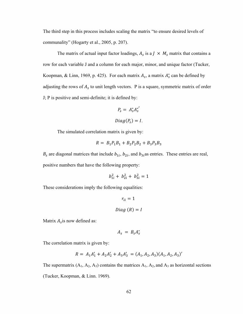
62
The third step in this process includes scaling the matrix “to ensure desired levels of
communality” (Hogarty et al., 2005, p. 207).
The matrix of actual input factor loadings, is a matrix that contains a
row for each variable J and a column for each major, minor, and unique factor (Tucker,
Koopman, & Linn, 1969, p. 425). For each matrix , a matrix ∗ can be defined by
adjusting the rows of to unit length vectors. P is a square, symmetric matrix of order
J; P is positive and semi-definite; it is defined by:
∗ ∗
.
The simulated correlation matrix is given by:
are diagonal matrices that include , , and as entries. These entries are real,
positive numbers that have the following property:
1
These considerations imply the following equalities:
1
Matrix is now defined as:
∗
The correlation matrix is given by:
, , , , ′
The supermatrix (A1, A2, A3) contains the matrices A1, A2, and A3 as horizontal sections
(Tucker, Koopman, & Linn. 1969).

63
The coefficients in the Bs matrices “regulate” the amount of variability in the
variables that is related to the major, minor, and unique factors. The matrix contains
communalities, and the contain values for uniqueness. When B2 matrix is zero, the
“simulation model” equals the “formal model” (Tucker, Koopman, & Linn, 1969, p.
426).
This study included the formal model as the simulation model. The B2 matrix is
set to zero, and by implication, the input factor loadings for minor factors were zero.
This forced the “data generation model” to match “a factor analytic model” with the
number of common factors equal to the levels specified for each combination of research
contexts that was examined in this study. This study included two, four, and eight
common factors.
Illustrative Example for Generating a Correlation Matrix
This illustration of the process for generating population correlation matrices
includes nine variables and three common factors. In this simulated factor model, the
communalities range from 0.6 to 0.8. Table 1 presents the matrix of conceptual factor
input loadings, , that is employed in this illustration. Note that the first conceptual
factor loading for each observed variable was assigned randomly; the sum of the
conceptual loadings for each variable is two.
As described in the previous section, translating this matrix of conceptual factor
input loadings into a matrix of actual input loadings requires the incorporation of
variation and discrepancies that mimic realistic instruments and studies. This process
includes random normal deviates, constants for each factor, and a constant for each

64
variable. Tables 2, 3, 4, and 5 illustrate the components associated with the second step
in developing the matrix of actual input loadings.
Table 1 Matrix of Relative Conceptual Factor Input Loadings, Variable Factor 1 Factor 2 Factor 3
1 0 1 1
2 2 0 0
3 0 2 0
4 2 0 0
5 0 0 2
6 0 1 1
7 2 0 0
8 1 0 1
9 2 0 0
Table 2 contains a matrix of random normal deviates, . When combined with
the vector of normalizing constants for each factor, , the 9 x 3 matrix of random
normal deviates is reduced to a unit length vector.
The normalizing coefficients, , for the random deviates included in this
illustration are given in Table 3. Tucker, Koopman, and Linn’s (1969) procedure for
simulating natural variation includes a matrix of constants, , for each major factor;
this formula for also includes the squared values of these constants.

65
Table 2
Matrix of Random Normal Deviates
Variable Factor 1 Factor 2 Factor 3
1 0.699 1.078 0.043
2 1.056 0.950 1.669
3 0.385 0.151 -0.971
4 -0.687 -0.590 -1.156
5 0.040 1.016 -1.560
6 -1.133 1.162 1.269
7 1.208 1.356 -0.129
8 1.266 -0.932 -0.201
9 1.603 0.088 04.435
Table 3 Values for the Coefficients Variable Value
1 0.778
2 0.456
3 0.947
4 0.681
5 0.537
6 0.485
7 0.549
8 0.631
9 0.601
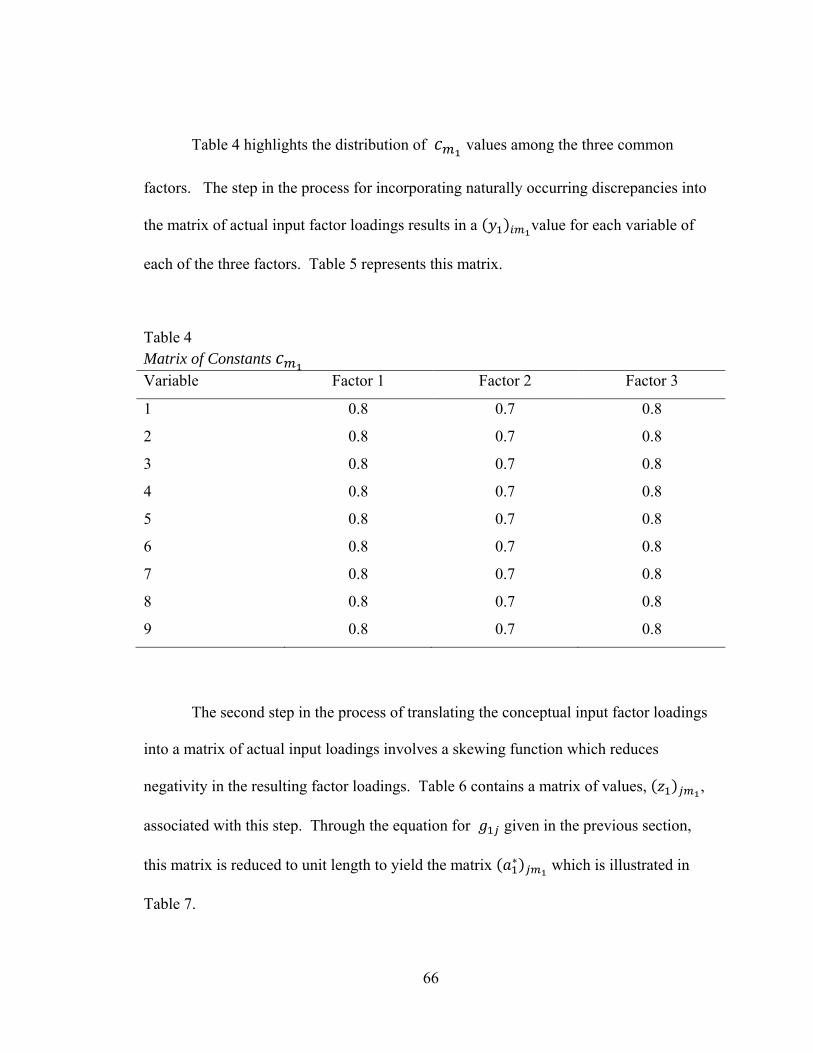
66
Table 4 highlights the distribution of values among the three common
factors. The step in the process for incorporating naturally occurring discrepancies into
the matrix of actual input factor loadings results in a value for each variable of
each of the three factors. Table 5 represents this matrix.
Table 4 Matrix of Constants Variable Factor 1 Factor 2 Factor 3
1 0.8 0.7 0.8
2 0.8 0.7 0.8
3 0.8 0.7 0.8
4 0.8 0.7 0.8
5 0.8 0.7 0.8
6 0.8 0.7 0.8
7 0.8 0.7 0.8
8 0.8 0.7 0.8
9 0.8 0.7 0.8
The second step in the process of translating the conceptual input factor loadings
into a matrix of actual input loadings involves a skewing function which reduces
negativity in the resulting factor loadings. Table 6 contains a matrix of values, ,
associated with this step. Through the equation for given in the previous section,
this matrix is reduced to unit length to yield the matrix ∗ which is illustrated in
Table 7.
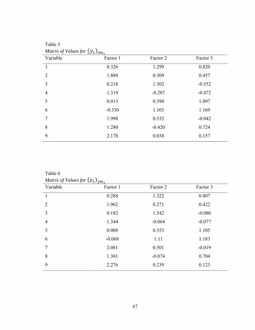
67
Table 5 Matrix of Values for Variable Factor 1 Factor 2 Factor 3
1 0.326 1.299 0.820
2 1.889 0.309 0.457
3 0.218 1.502 -0.552
4 1.319 -0.287 -0.472
5 0.013 0.390 1.097
6 -0.330 1.103 1.169
7 1.998 0.532 -0.042
8 1.280 -0.420 0.724
9 2.178 0.038 0.157
Table 6 Matrix of Values for Variable Factor 1 Factor 2 Factor 3
1 0.288 1.322 0.807
2 1.962 0.271 0.422
3 0.182 1.542 -0.080
4 1.344 -0.064 -0.077
5 0.008 0.353 1.105
6 -0.068 1.11 1.183
7 2.081 0.501 -0.019
8 1.301 -0.074 0.704
9 2.276 0.239 0.123
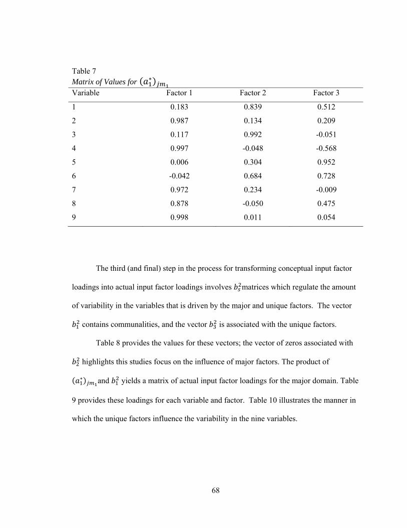
68
Table 7 Matrix of Values for ∗ Variable Factor 1 Factor 2 Factor 3
1 0.183 0.839 0.512
2 0.987 0.134 0.209
3 0.117 0.992 -0.051
4 0.997 -0.048 -0.568
5 0.006 0.304 0.952
6 -0.042 0.684 0.728
7 0.972 0.234 -0.009
8 0.878 -0.050 0.475
9 0.998 0.011 0.054
The third (and final) step in the process for transforming conceptual input factor
loadings into actual input factor loadings involves matrices which regulate the amount
of variability in the variables that is driven by the major and unique factors. The vector
contains communalities, and the vector is associated with the unique factors.
Table 8 provides the values for these vectors; the vector of zeros associated with
highlights this studies focus on the influence of major factors. The product of
∗ and yields a matrix of actual input factor loadings for the major domain. Table
9 provides these loadings for each variable and factor. Table 10 illustrates the manner in
which the unique factors influence the variability in the nine variables.

69
Table 8 Values of b2 Coefficients,
Variable
1 0.7 0.0 0.3
2 0.6 0.0 0.4
3 0.7 0.0 0.3
4 0.7 0.0 0.3
5 0.8 0.0 0.2
6 0.8 0.0 0.2
7 0.8 0.0 0.2
8 0.6 0.0 0.4
9 0.6 0.0 0.4
Table 9 Matrix of Actual Factor Input Loadings for the Major Domain, A1
Variable Factor 1 Factor 2 Factor 3
1 0.153 0.702 0.428
2 0.750 0.104 0.162
3 0.098 0.830 -0.043
4 0.834 -0.040 -0.047
5 0.005 0.272 0.852
6 -0.037 0.612 0.651
7 0.869 0.209 -0.008
8 0.680 -0.039 0.368
9 0.773 0.008 0.042

70
Table 10 Values for Factor Input Loadings for the Unique Factors, A3 Variable Value
1 0.548
2 0.632
3 0.548
4 0.548
5 0.447
6 0.447
7 0.447
8 0.632
9 0.632
Table 11 presents the correlation matrix that is a result of the sum of products of the A1
matrix with its inverse and the A3 with its inverse.
Table 11 Simulated Correlations Variable 1 2 3 4 5 6 7 8 9
1 .257 .579 .080 .557 .703 .277 .235 .142
2 .152 .614 .170 .141 .673 .566 .588
3 .500 .190 .476 .259 .186 .080
4 -.465 -.087 .717 .552 .643
5 .721 .055 .307 .191
6 .090 .191 .003
7 .581 .674
8 .541
9
71
This simulation was developed in SAS 9.2. The IML code was adapted from a
study conducted by Hogarty, Hines, Kromrey, Ferron, and Mumford (2005). The
program associated with this design example can be found in Appendix B.
Monte Carlo Simulation Design
With few modifications, the simulation strategy included in this study is derived
from Hogarty, Hines, Kromrey, Ferron, & Mumford’s (2005) investigation of the
relationship between sample size and factor solutions. The primary modification includes
the addition of various proportions of categorical variables to the simulated data sets.
This study also controlled for the number of variables, communality levels, and sample
size.
Proportion of categorical variables. The ratios of categorical to continuous
variables are selected to provide insight into a variety of research contexts. The samples
developed through the simulated correlation matrices included distributions that
contained the following percentages of categorical variables: 5%, 25%, 50%, 75%, and
95%. While simulating a broad range of data contexts, these percentages resulted in
whole numbers of variables in data sets that contain 20, 40, and 60 observed variables.
During the data generation phase of this design, differing percentages of each
sample of observed variables were dichotomized to yield the appropriate number of
categorical observations. When data were intended to represent categorical variables, the
resulting, simulated value was dichotomized at 0.5. When the value was less than 0.5,
the value of the categorical variable was set to zero; when the value was greater than or
equal to 0.5, the value of the categorical value was set to one.

72
Number of variables. To enhance this project’s generalizability, this study
included simulations of results from data sets of varying size. When considered in
concert with the differing sample sizes, this study incorporated participant (N) to variable
(p) ratios that range from “insufficient to those considered more than acceptable”
(MacCallum, Widaman, Zhang, & Hong, 1999, p. 92). This study simulated data sets
containing 20, 40, and 60 variables. The simulated combinations of sample sizes and
numbers of observed variables yileded N: p ratios that range from 1.67:1 to 30:1.
Number of common factors. This study simulated research contexts that involve
varying ratios of observed variables to common factors. The number of factors condition
consisted of three levels: two, four, and eight common factors. Because factors defined
by fewer than two variables would “contradict the basic idea of a factor as a latent
construct” (Henson & Roberts, p. 408), the upper limit on the number of common factors
simulated in this study was constrained by the simulated context which includes 20
observed variables. In this study, the ratio of observed variables to common factors
ranged from 2.5:1, or insufficient (Fabrigar et al., 1999), to 30:1.
Communality levels. The simulated levels of communality included in this study
are also derived from existing methodological research in factor analysis. This study
simulated three community levels: high, wide, and low communality (h2) (Hogarty et al.,
2005; MacCallum, Widaman, Zhang, & Hong, 1999). These communality levels
correspond to the following:
1. High--h2 for each variable are randomly drawn from values of .6, .7, and .8
2. Wide--h2 for each variable are randomly drawn from values of .2, .3, .4, .5, .6, .7,
and .8

73
3. Low--h2 for each variable are randomly drawn from values of .2, .3, and .4
Sample size. The four sample size (N) conditions included in this study were 100,
200, 300, and 1000 simulated subjects. Although many studies provide suggested
minimum values for the ratio of participants to variables when employing factor analytic
techniques (Stevens, 2002), recent simulation studies do not find a minimum sample size
to variable ratio that can be associated with good factor recovery (Hogarty et al., 2005;
MacCallum, Widaman, Zhang, & Hong, 1999). Therefore, the sample size levels
included in this study are based on ranges of sample sizes that are commonly found in
recent factor analytic research in organizational management and social science research
(Conway & Huffcutt, 2003).
Rotation. The initial factor solutions from each model in each condition was
subjected to an orthogonal rotation strategy. Specifically, this study employed a varimax
rotation in all simulated contexts. Because the intent of this study is to address
methodological issues that are frequently encountered in social science literature,
varimax rotation was considered to be a more appropriate choice than the
methodologically sound procustrean rotation (Fabrigar et al., 1999; Merrifield, 1974;
Raykov & Little, 1999). The parsimony associated with uncorrelated factors represents
one of the strongest rationales for employing orthogonal rotation strategies (Fabrigar et
al., 1999; Raykov & Little, 1999).
Evaluation of Factor Extraction Methods
Principal axis, ordinary least squares, and maximum likelihood factor extraction
methods were evaluated in terms of five general sets of criteria. These criteria include:
population and sample factor pattern agreement, congruence, and correlations between

74
population and sample factor score matrices. (Hogarty et al., 2005; MacCallum,
Widaman, Zhang, & Hong, 1999). The following sections address each of these
evaluation criteria.
Population and sample factor pattern agreement. This study includes
assessments of agreement between the population, or true, factor characteristics and those
characteristics implied by the factor analytic techniques under investigation, the sample.
These measures were also described by Hogarty, Hines, Kromrey, Ferron, and Mumford
(2005), and they include:
1. Loading sensitivity or agreement between sample and population in terms of the
proportion of variables that have factor pattern coefficients that are greater than or
equal to .30 on at least one factor; this indicator measures the level of agreement
between sample and population matrices in terms of variables that load on at least
one factor (Hogarty et al., 2005).
2. General pattern agreement as measured by the proportion of samples in which all
of the variables loaded on the same factors in both the sample and the population.
This measure does not take into account the magnitude of variable loadings on
other factors in the sample matrices. “This index represents the extent of
agreement for all variables that load on at least on factor” (Hogarty et al., 2005, p.
209).
3. Total agreement between sample and population is expressed in terms of the
proportion of samples in which all variables loaded on sample and a population
factors to the same extent. Factor loadings will be assessed as agreeing if both
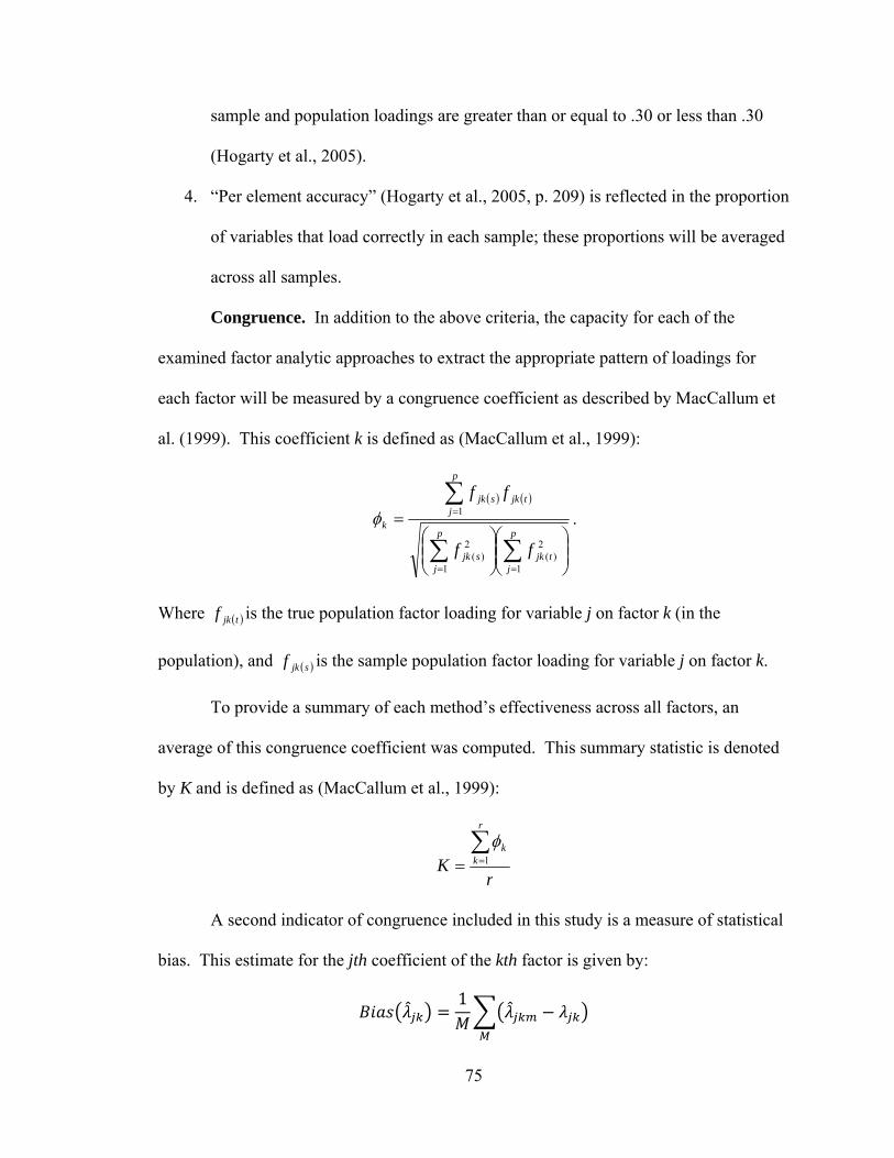
75
sample and population loadings are greater than or equal to .30 or less than .30
(Hogarty et al., 2005).
4. “Per element accuracy” (Hogarty et al., 2005, p. 209) is reflected in the proportion
of variables that load correctly in each sample; these proportions will be averaged
across all samples.
Congruence. In addition to the above criteria, the capacity for each of the
examined factor analytic approaches to extract the appropriate pattern of loadings for
each factor will be measured by a congruence coefficient as described by MacCallum et
al. (1999). This coefficient k is defined as (MacCallum et al., 1999):
p
jtjk
p
jsjk
p
jtjksjk
k
ff
ff
1
2)(
1
2)(
1 .
Where tjkf is the true population factor loading for variable j on factor k (in the
population), and sjkf is the sample population factor loading for variable j on factor k.
To provide a summary of each method’s effectiveness across all factors, an
average of this congruence coefficient was computed. This summary statistic is denoted
by K and is defined as (MacCallum et al., 1999):
rK
r
kk
1
A second indicator of congruence included in this study is a measure of statistical
bias. This estimate for the jth coefficient of the kth factor is given by:
1

76
Where is the coefficient obtained via the mth sample, is the population
coefficient, and M is the number of samples included in the study. The absolute values of
bias will be used in the computation of an average across the M samples (Hogarty et al.,
2005).
The third indicator of congruence included in this study was the root mean square
error (RMSE). The estimate of RMSE is given by:
1
The elements included in the estimate of RMSE are identical to those used to estimate a
value for bias.
Correlations between population and sample factor score matrices. The first
step in developing this evaluation measure includes the development of factor score
estimates. These score estimates are linear combinations of variables; however, as
opposed to using factor score coefficients, these estimates were computed using the
following process:
1. A positive one scoring coefficient is assigned when the observed structure
coefficient is .30;
2. A negative one scoring coefficient is assigned when the observed structure
coefficient is .30;
3. A scoring coefficient of zero is assigned when the structure coefficient is between
.30 and -.30.
Ater factor scores estimates werere computed for both the population and sample
matrices, a correlation among the scores was used to measure how closely factor scores
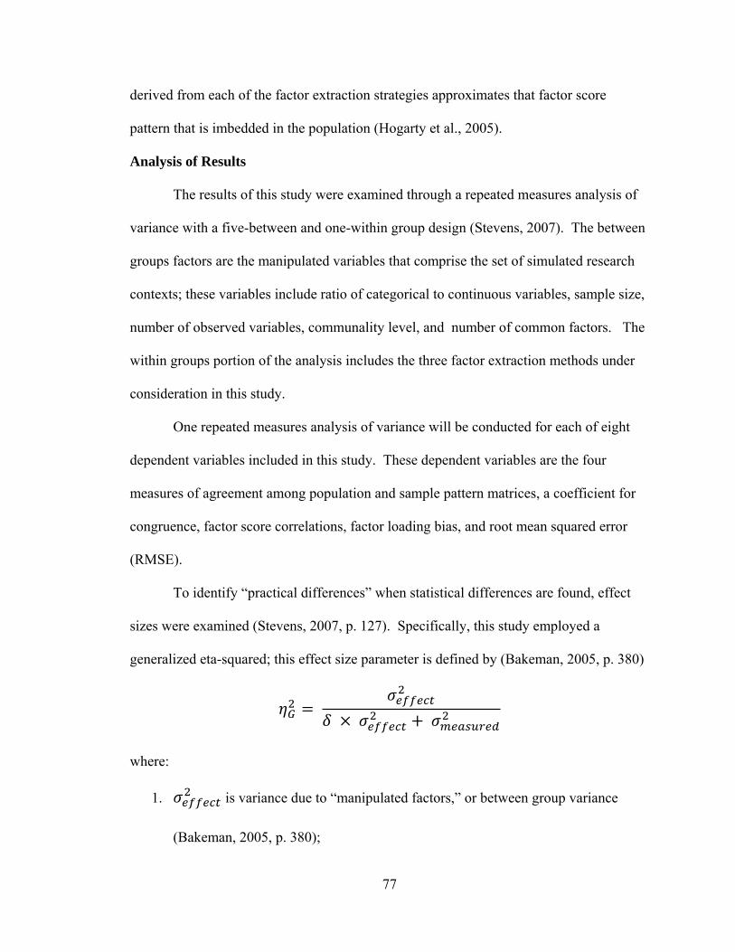
77
derived from each of the factor extraction strategies approximates that factor score
pattern that is imbedded in the population (Hogarty et al., 2005).
Analysis of Results
The results of this study were examined through a repeated measures analysis of
variance with a five-between and one-within group design (Stevens, 2007). The between
groups factors are the manipulated variables that comprise the set of simulated research
contexts; these variables include ratio of categorical to continuous variables, sample size,
number of observed variables, communality level, and number of common factors. The
within groups portion of the analysis includes the three factor extraction methods under
consideration in this study.
One repeated measures analysis of variance will be conducted for each of eight
dependent variables included in this study. These dependent variables are the four
measures of agreement among population and sample pattern matrices, a coefficient for
congruence, factor score correlations, factor loading bias, and root mean squared error
(RMSE).
To identify “practical differences” when statistical differences are found, effect
sizes were examined (Stevens, 2007, p. 127). Specifically, this study employed a
generalized eta-squared; this effect size parameter is defined by (Bakeman, 2005, p. 380)
where:
1. is variance due to “manipulated factors,” or between group variance
(Bakeman, 2005, p. 380);

78
2. is equal to one if the effect includes only factors that are manipulated by the
investigator;
3. includes variance due to individual differences (Bakeman, 2005);
In addition to the summary tables associated with balanced, between groups,
factorial analyses of variance, results of this study are presented graphically. When
statistically significant differences among factor extraction methods were identified, the
Tukey procedure was employed to identify the sources of these significant differences.

Chapter Four
79
Results
The intent of this study is to explore the extent to which characteristics of factor
models derived through the tested factor analytic methods agree with the true
characteristics simulated in the population. Because of the explorative nature of this
study, it will include both multivariate and univariate approaches to the repeated
measures analysis; this approach can identify sets of significant treatment effects that
neither approach may resolve on its own (Stevens, 2002, 2007). To accommodate for
increased experiment-wise, type I error rates, tests of significance are based on .025 alpha
level
Table 12 provides means and standard deviations of all performance measures by
factor extraction method; these measures include factor loading sensitivity, general
pattern agreement, per element agreement, total pattern agreement of agreement,
congruence, factor score correlations, bias, and root mean squared error (RMSE). As the
table indicates, mean values of total agreement are near zero for all tested factor
extraction methods. In the two factor by 60 observed variable condition, principal axis
and maximum likelihood factor extraction methods yielded factor score estimates of zero;
therefore factor score correlations for these conditions could not be calculated
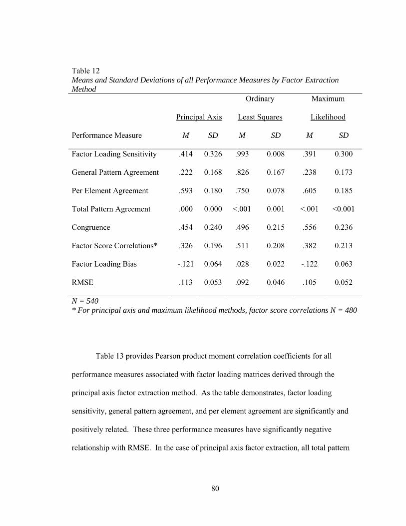
80
Table 12 Means and Standard Deviations of all Performance Measures by Factor Extraction Method
Principal Axis
Ordinary
Least Squares
Maximum
Likelihood
Performance Measure M SD M SD M SD
Factor Loading Sensitivity .414 0.326 .993 0.008 .391 0.300
General Pattern Agreement .222 0.168 .826 0.167 .238 0.173
Per Element Agreement .593 0.180 .750 0.078 .605 0.185
Total Pattern Agreement .000 0.000 <.001 0.001 <.001 <0.001
Congruence .454 0.240 .496 0.215 .556 0.236
Factor Score Correlations* .326 0.196 .511 0.208 .382 0.213
Factor Loading Bias -.121 0.064 .028 0.022 -.122 0.063
RMSE .113 0.053 .092 0.046 .105 0.052
N = 540 * For principal axis and maximum likelihood methods, factor score correlations N = 480 Table 13 provides Pearson product moment correlation coefficients for all
performance measures associated with factor loading matrices derived through the
principal axis factor extraction method. As the table demonstrates, factor loading
sensitivity, general pattern agreement, and per element agreement are significantly and
positively related. These three performance measures have significantly negative
relationship with RMSE. In the case of principal axis factor extraction, all total pattern
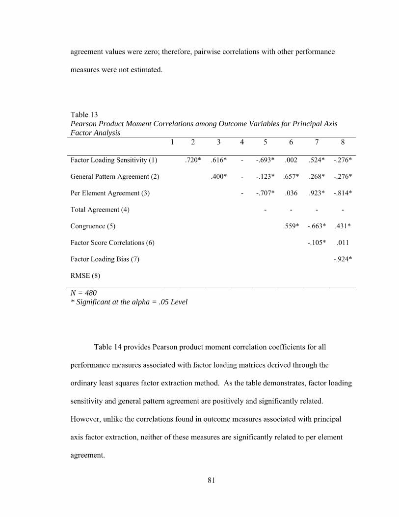
81
agreement values were zero; therefore, pairwise correlations with other performance
measures were not estimated.
Table 13 Pearson Product Moment Correlations among Outcome Variables for Principal Axis Factor Analysis 1 2 3 4 5 6 7 8
Factor Loading Sensitivity (1) .720* .616* - -.693* .002 .524* -.276*
General Pattern Agreement (2) .400* - -.123* .657* .268* -.276*
Per Element Agreement (3) - -.707* .036 .923* -.814*
Total Agreement (4) - - - -
Congruence (5) .559* -.663* .431*
Factor Score Correlations (6) -.105* .011
Factor Loading Bias (7) -.924*
RMSE (8)
N = 480 * Significant at the alpha = .05 Level
Table 14 provides Pearson product moment correlation coefficients for all
performance measures associated with factor loading matrices derived through the
ordinary least squares factor extraction method. As the table demonstrates, factor loading
sensitivity and general pattern agreement are positively and significantly related.
However, unlike the correlations found in outcome measures associated with principal
axis factor extraction, neither of these measures are significantly related to per element
agreement.
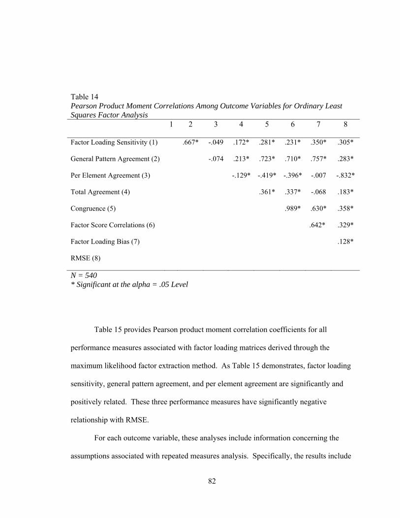
82
Table 14 Pearson Product Moment Correlations Among Outcome Variables for Ordinary Least Squares Factor Analysis 1 2 3 4 5 6 7 8
Factor Loading Sensitivity (1) .667* -.049 .172* .281* .231* .350* .305*
General Pattern Agreement (2) -.074 .213* .723* .710* .757* .283*
Per Element Agreement (3) -.129* -.419* -.396* -.007 -.832*
Total Agreement (4) .361* .337* -.068 .183*
Congruence (5) .989* .630* .358*
Factor Score Correlations (6) .642* .329*
Factor Loading Bias (7) .128*
RMSE (8)
N = 540 * Significant at the alpha = .05 Level
Table 15 provides Pearson product moment correlation coefficients for all
performance measures associated with factor loading matrices derived through the
maximum likelihood factor extraction method. As Table 15 demonstrates, factor loading
sensitivity, general pattern agreement, and per element agreement are significantly and
positively related. These three performance measures have significantly negative
relationship with RMSE.
For each outcome variable, these analyses include information concerning the
assumptions associated with repeated measures analysis. Specifically, the results include
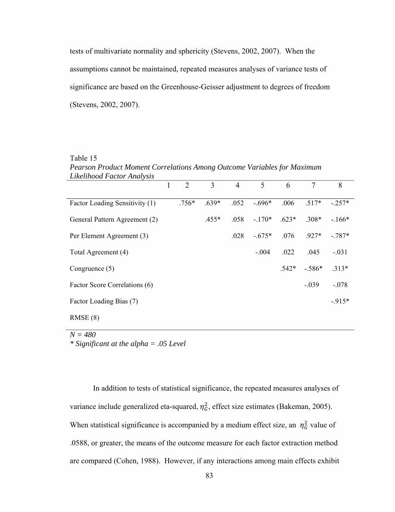
83
tests of multivariate normality and sphericity (Stevens, 2002, 2007). When the
assumptions cannot be maintained, repeated measures analyses of variance tests of
significance are based on the Greenhouse-Geisser adjustment to degrees of freedom
(Stevens, 2002, 2007).
Table 15 Pearson Product Moment Correlations Among Outcome Variables for Maximum Likelihood Factor Analysis 1 2 3 4 5 6 7 8
Factor Loading Sensitivity (1) .756* .639* .052 -.696* .006 .517* -.257*
General Pattern Agreement (2) .455* .058 -.170* .623* .308* -.166*
Per Element Agreement (3) .028 -.675* .076 .927* -.787*
Total Agreement (4) -.004 .022 .045 -.031
Congruence (5) .542* -.586* .313*
Factor Score Correlations (6) -.039 -.078
Factor Loading Bias (7) -.915*
RMSE (8)
N = 480 * Significant at the alpha = .05 Level
In addition to tests of statistical significance, the repeated measures analyses of
variance include generalized eta-squared, , effect size estimates (Bakeman, 2005).
When statistical significance is accompanied by a medium effect size, an value of
.0588, or greater, the means of the outcome measure for each factor extraction method
are compared (Cohen, 1988). However, if any interactions among main effects exhibit

84
the same pattern of statistical significance and effect size, then only the interaction are
interpreted. Comparisons among means are considered through tables, graphs of means,
and box and whisker plots.
Factor Loading Sensitivity
Factor loading sensitivity is expressed in terms of agreement between sample and
population in terms of the proportion of variables that have factor pattern coefficients that
are greater than or equal to .30 on at least one factor. This is the count of variables that
meet a .30 factor loading threshold for at least one factor in both the sample and the
population divided by the count of variables that meet the .30 loading threshold in the
population. Table 16 presents descriptive statistics concerning the univariate distribution
of this loading sensitivity measure by each of the tested factor extraction methods.
Table 16 Descriptive Statistics for Distribution of Factor Loading Sensitivity Values Factor Extraction Method N M SD Skewness Kurtosis
Principal Axis 540 0.414 0.326 0.305 -1.130
Ordinary Least Squares 540 0.993 0.008 -1.122 0.158
Maximum Likelihood 540 0.391 0.300 0.254 -1.120
When combined with the observed levels of skewness and Kurtosis, the Shapiro-
Wilk tests of normality provide evidence of significant non-normality in the univariate

85
distributions of factor loading sensitivity measures for all three factor extraction methods.
Moreover, Mauchly’s test of transformed variables, (2) = 337.428, p < .0001, indicate
that the data do not conform to the sphericity assumption associated with repeated
measures ANOVA. To account for these violations of the assumptions associated with
the univariate, repeated measures analysis of variance, the Greenhouse-Geisser
adjustment to degrees of freedom was used to develop p values for the within subjects
tests of significance.
The multivariate analysis of variance indicate that factor loading sensitivity
differed significantly by factor extraction method, Λ = .0001, F (2, 495) = 342901, p <
.0001. In addition to the factor extraction method main effect, all interaction among
factor extraction method and manipulated research characteristics yielded significant
differences in factor loading sensitivity. Eight of the 10 first order interactions among
main effects are also significant at the alpha = 0.025 level. The results of these analyses
can be found in see Table C1 (see appendix C).
Results of the repeated analysis of variance yield a similar pattern of significance
as those associated with the multivariate analysis. For example, the within-subjects
portion of the ANOVA indicate that mean values of factor loading sensitivity differ
significantly by factor extraction method, F (2, 920) = 600815, p < .0001, = .999.
The model including main effects and first-order interactions accounted for 99.9% of the
variability associated with factor loading sensitivity.
In addition to the method effect, the between subjects analysis yielded evidence
that the sensitivity measure differed significantly for all of the main effects: Number of
factors (K), number of observed variables (P), sample size (N), communality range (H),

86
and dichotomization (D). The results also indicate that mean values of this measure were
significantly related to five interactions among these main effects; these interactions
include number of factors by number of observed variables (K × P), number of factors by
communality range (K × H), number of factors by level of dichotomization (K × D),
number of observed variables by communality range (P × H), and communality range by
level of dichotomization (H × D). The results of the univariate, repeated measures
ANOVA can be found in C2 (see appendix C).
Agreement between the multivariate and univariate approaches was not universal.
The multivariate approach yielded evidence that factor loading sensitivity is significantly
related to interactions between number of observed variables by sample size (P × N) and
number of observed variables by level of dichotomization (P × D) (see Table C1 in
appendix C). However, the univariate, repeated measures analysis failed to yield
evidence of significant differences in mean levels of factor loading sensitivity associated
with these interactions.
Because the generalized eta-squared values for the P × N and P × D interactions
indicated that their effect sizes were less than medium (Cohen, 1988), comparisons
among the mean values for factor loading sensitivity based on these interactions were not
analyzed. Although each main effect is also included in a first-order interaction that
yielded a medium or greater effect size, this study includes interpretations of the
interaction effects only. The two interactions with factor extraction methods that met
both the statistical significance and the effect size requirements for further analyses
include number of factors by number of observed variables, F (8, 920) = 1086.34, p <
.0001, = .862, and number of observed variables by communality range, F (8, 920) =
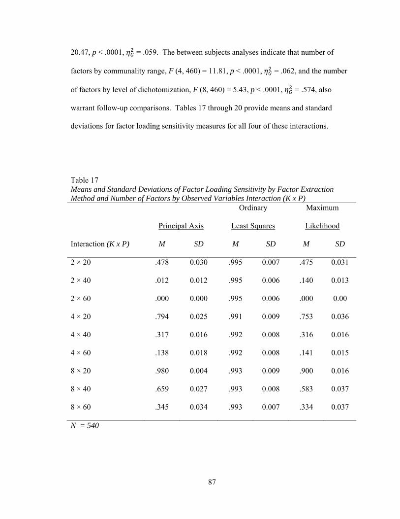
87
20.47, p < .0001, = .059. The between subjects analyses indicate that number of
factors by communality range, F (4, 460) = 11.81, p < .0001, = .062, and the number
of factors by level of dichotomization, F (8, 460) = 5.43, p < .0001, = .574, also
warrant follow-up comparisons. Tables 17 through 20 provide means and standard
deviations for factor loading sensitivity measures for all four of these interactions.
Table 17 Means and Standard Deviations of Factor Loading Sensitivity by Factor Extraction Method and Number of Factors by Observed Variables Interaction (K x P)
Principal Axis
Ordinary
Least Squares
Maximum
Likelihood
Interaction (K x P) M SD M SD M SD
2 × 20 .478 0.030 .995 0.007 .475 0.031
2 × 40 .012 0.012 .995 0.006 .140 0.013
2 × 60 .000 0.000 .995 0.006 .000 0.00
4 × 20 .794 0.025 .991 0.009 .753 0.036
4 × 40 .317 0.016 .992 0.008 .316 0.016
4 × 60 .138 0.018 .992 0.008 .141 0.015
8 × 20 .980 0.004 .993 0.009 .900 0.016
8 × 40 .659 0.027 .993 0.008 .583 0.037
8 × 60 .345 0.034 .993 0.007 .334 0.037
N = 540
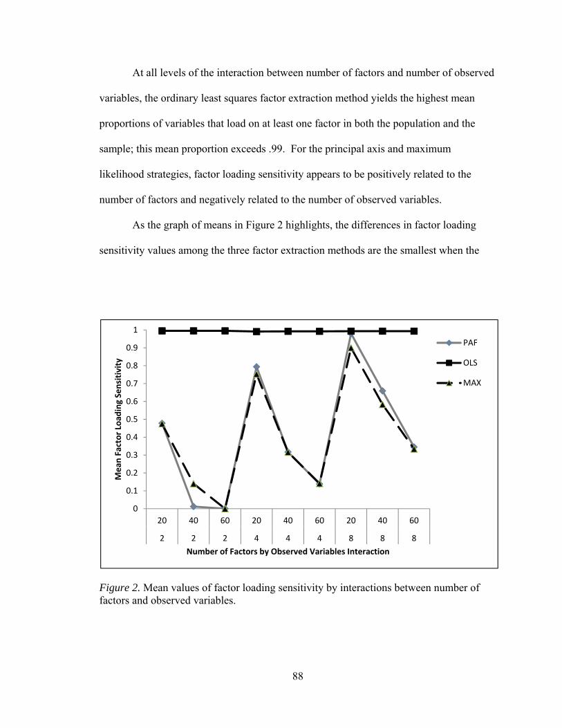
88
At all levels of the interaction between number of factors and number of observed
variables, the ordinary least squares factor extraction method yields the highest mean
proportions of variables that load on at least one factor in both the population and the
sample; this mean proportion exceeds .99. For the principal axis and maximum
likelihood strategies, factor loading sensitivity appears to be positively related to the
number of factors and negatively related to the number of observed variables.
As the graph of means in Figure 2 highlights, the differences in factor loading
sensitivity values among the three factor extraction methods are the smallest when the
Figure 2. Mean values of factor loading sensitivity by interactions between number of factors and observed variables.
0
0.1
0.2
0.3
0.4
0.5
0.6
0.7
0.8
0.9
1
20 40 60 20 40 60 20 40 60
2 2 2 4 4 4 8 8 8
Mean
Factor Load
ing Sensitivity
Number of Factors by Observed Variables Interaction
PAF
OLS
MAX

89
observed variable to factor ratio is the smallest. Box and whisker plots of these mean
proportions indicate that factor loading sensitivity values associated with the least squares
have smaller ranges and semi-interquartile ranges than the distributions associated with
maximum likelihood and principal axis factor extraction methods (see Figure D1 in
appendix D). For the ordinary least squares factor extraction method, measures of both
central tendency and dispersion in the distributions of factor loading sensitivity values
appear to be independent of observed variable to number of factor ratios.
Table 18 provides means and standard deviations of factor loading sensitivity
values based on the number of factors by communality range interaction. The ordinary
least squares factor extraction method yields the highest mean proportions of variables
that load on at least one factor in both the population and the sample. For the principal
axis and maximum likelihood strategies, the measure of factor loading sensitivity is
positively related to both the number of factors and community level. Mean values of
factor loading sensitivity associated with the Ordinary Least Squares factor extraction
method appeared to be independent of a K × H interaction effect values. As the graph of
means in Figure 3 indicates, the differences in factor loading sensitivity decrease as
number of factors and communality range increase.
Box and whisker plots indicate that factor loading sensitivity values associated
with the least squares have smaller ranges and semi-interquartile ranges than the
distributions associated with maximum likelihood and principal axis factor extraction
methods (see Figure D2 in appendix D). For the ordinary least squares factor extraction
method, measures of both central tendency and dispersion in the distributions of factor

90
loading sensitivity values appear to be independent of levels of the number of factors by
communality interaction.
Table 18 Means and Standard Deviations of Factor Loading Sensitivity by Factor Extraction Method and Number of Factors by Communality Range Interaction (K x H)
Principal Axis
Ordinary
Least Squares
Maximum
Likelihood
Interaction (K x H) M SD M SD M SD
2 × Low .155 0.214 .999 0.007 .154 0.212
2 × Wide .165 0.217 .996 0.003 .165 0.214
2 × High .170 0.243 1.000 0.000 .170 0.242
4 × Low .409 0.289 .982 0.006 .390 0.259
4 × Wide .412 0.266 .993 0.002 .398 0.246
4 × High .429 0.284 .999 0.000 .422 0.276
8 × Low .651 0.273 .982 0.005 .584 0.242
8 × Wide .655 0.264 .996 0.002 .600 0.233
8 × High .678 0.250 .999 0.000 .635 0.231
N = 540 Note:
Table 19 presents means and standard deviations of factor loading sensitivity
values based on the number of factors by level of dichotomization interaction (K × D).

91
Across all levels of the interaction, factor loading sensitivity is highest for the Ordinary
Least Squares factor extraction method.
Figure 3. Mean values of factor loading sensitivity by interactions between number of factors and communality.
For the principal axis and maximum likelihood strategies, values of the factor loading
sensitivity measure are positively related to the number of factors. For each number of
factors level, the mean values for factor loading sensitivity increase in value between the
.05 and .75 levels of dichotomization. However, for each combination of effects, the
mean factor loading sensitivity value decreases between the .75 and .95 dichotomization
levels.
0
0.1
0.2
0.3
0.4
0.5
0.6
0.7
0.8
0.9
1
Low Wide High Low Wide High Low Wide High
2 2 2 4 4 4 8 8 8
Mean
Factor Load
ing Sensitivity
Number of Factors by Communality Level Interaction
PAF
OLS
MAX
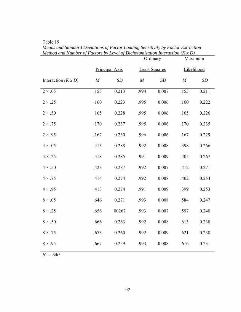
92
Table 19 Means and Standard Deviations of Factor Loading Sensitivity by Factor Extraction Method and Number of Factors by Level of Dichotomization Interaction (K x D)
Principal Axis
Ordinary
Least Squares
Maximum
Likelihood
Interaction (K x D) M SD M SD M SD
2 × .05 .155 0.213 .994 0.007 .155 0.211
2 × .25 .160 0.223 .995 0.006 .160 0.222
2 × .50 .165 0.228 .995 0.006 .165 0.226
2 × .75 .170 0.237 .995 0.006 .170 0.235
2 × .95 .167 0.230 .996 0.006 .167 0.229
4 × .05 .413 0.288 .992 0.008 .398 0.266
4 × .25 .418 0.285 .991 0.009 .405 0.267
4 × .50 .423 0.287 .992 0.007 .412 0.271
4 × .75 .414 0.274 .992 0.008 .402 0.254
4 × .95 .413 0.274 .991 0.009 .399 0.253
8 × .05 .646 0.271 .993 0.008 .584 0.247
8 × .25 .656 00267 .993 0.007 .597 0.240
8 × .50 .666 0.263 .992 0.008 .613 0.238
8 × .75 .673 0.260 .992 0.009 .621 0.230
8 × .95 .667 0.259 .993 0.008 .616 0.231
N = 540
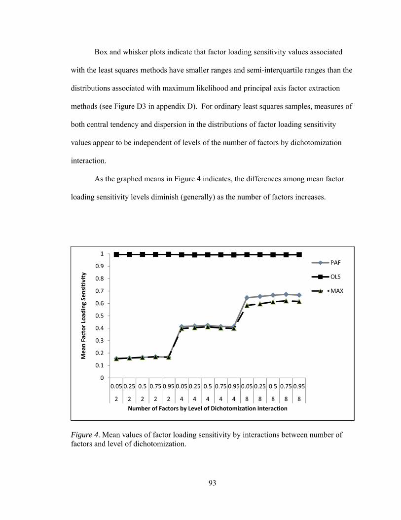
93
Box and whisker plots indicate that factor loading sensitivity values associated
with the least squares methods have smaller ranges and semi-interquartile ranges than the
distributions associated with maximum likelihood and principal axis factor extraction
methods (see Figure D3 in appendix D). For ordinary least squares samples, measures of
both central tendency and dispersion in the distributions of factor loading sensitivity
values appear to be independent of levels of the number of factors by dichotomization
interaction.
As the graphed means in Figure 4 indicates, the differences among mean factor
loading sensitivity levels diminish (generally) as the number of factors increases.
Figure 4. Mean values of factor loading sensitivity by interactions between number of factors and level of dichotomization.
0
0.1
0.2
0.3
0.4
0.5
0.6
0.7
0.8
0.9
1
0.05 0.25 0.5 0.75 0.95 0.05 0.25 0.5 0.75 0.95 0.05 0.25 0.5 0.75 0.95
2 2 2 2 2 4 4 4 4 4 8 8 8 8 8
Mean
Factor Load
ing Sensitivity
Number of Factors by Level of Dichotomization Interaction
PAF
OLS
MAX

94
The number of factors by level of dichotomization interaction effect does not appear to
have a substantial impact on the mean values of factor loading sensitivity associated with
the Ordinary Least Squares factor extraction method.
Mean values for factor loading sensitivity associated with the interaction among
numbers of observed variables and communality (P × H) are presented in Table 20.
Table 20 Means and Standard Deviations of Factor Loading Sensitivity by Factor Extraction Method and Number of Observed Variables by Communality Range Interaction (P x H)
Principal Axis
Ordinary
Least Squares
Maximum
Likelihood
Interaction (P x H) M SD M SD M SD
20 × Low .745 0.220 .983 0.008 .693 0.184
20 × Wide .739 0.211 .995 0.002 .696 0.179
20 × High .767 0.198 .999 0.001 .741 0.175
40 × Low .322 0.266 .985 0.007 .292 0.226
40 × Wide .329 0.256 .995 0.003 .307 0.225
40 × High .336 0.78 .999 0.000 .315 0.255
60 × Low .147 0.133 .986 0.006 .144 0.126
60 × Wide .162 0.140 .995 0.003 .160 0.138
60 × High .173 0.158 1.000 0.000 .170 0.155
n = 540
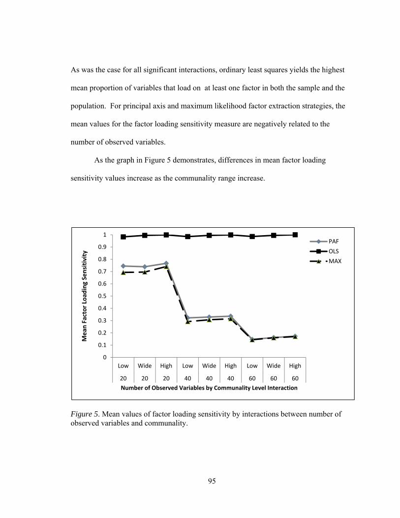
95
As was the case for all significant interactions, ordinary least squares yields the highest
mean proportion of variables that load on at least one factor in both the sample and the
population. For principal axis and maximum likelihood factor extraction strategies, the
mean values for the factor loading sensitivity measure are negatively related to the
number of observed variables.
As the graph in Figure 5 demonstrates, differences in mean factor loading
sensitivity values increase as the communality range increase.
Figure 5. Mean values of factor loading sensitivity by interactions between number of observed variables and communality.
0
0.1
0.2
0.3
0.4
0.5
0.6
0.7
0.8
0.9
1
Low Wide High Low Wide High Low Wide High
20 20 20 40 40 40 60 60 60
Mean
Factor Load
ing Sensitivity
Number of Observed Variables by Communality Level Interaction
PAF
OLS
MAX

96
Box and whisker plots indicate that factor loading sensitivity values associated
with ordinary least squares have smaller ranges and semi-interquartile ranges than the
distributions associated with maximum likelihood and principal axis factor extraction
methods (see Figure D4 in appendix D). For ordinary least squares samples, measures of
both central tendency and dispersion in the distributions of factor loading sensitivity
values appear to be independent of levels of the number of observed variables by
communality interaction.
Across all significant interactions among the manipulated research characteristics,
the ordinary least squares factor extraction method exhibited greater mean levels of factor
loading sensitivity than the principal axis and the maximum likelihood factor extraction
methods. Ordinary least squares factor extraction also resulted in distributions of factor
loading sensitivity that were less variable than the distributions associated with principal
axis and maximum likelihood. In interactions that included the number of factors main
effect, the differences in factor loading sensitivity between ordinary least squares and the
other two factor extraction methods were moderated by the number of factors; these
differences decreased as the number of factors increased.
General Pattern Agreement
General Pattern Agreement is based on the proportion of variables that load on
both the sample and population factors in a similar fashion at least once. This variable is
a P × 1 column vector. When the absolute value of a variable loading on the same factor
in both the sample and the population is greater than or equal to .30 at least once; then a
one is assigned to the row associated with the variable.
97
The proportion of variables that meet .30 loading criterion contributes to the
general pattern agreement. For this measure the variable can load on multiple factors and
still contribute to the pattern of agreement. Table 21 presents descriptive statistics
concerning the univariate distribution of the general pattern agreement measure by each
of the tested factor extraction methods.
Table 21 Descriptive Statistics for Distribution of General Pattern Agreement Factor Extraction Method N M SD Skewness Kurtosis
Principal Axis 540 .222 0.168 0.561 -0.443
Ordinary Least Squares 540 .826 0.167 -1.389 1.211
Maximum Likelihood 540 .238 0.173 0.470 -0.533
For all tested factor extraction methods, Shapiro Wilks’ tests of normality yield
evidence that the univariate distributions of general pattern accuracy values are not
normally distributed. Mauchly’s test of transformed variables, (2) = 600.964; p <
.0001, indicate that the data do not conform to the sphericity assumption associated with
repeated measures ANOVA. To address the potential for increased Type I error rate,
tests of significance associated with the repeated measures analysis of variance will be
based on the Greenhouse-Geisser adjustment to degrees of freedom (Stevens, 2002).
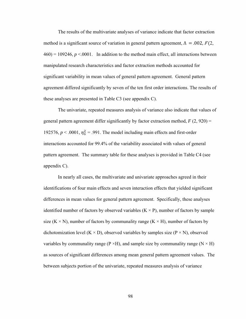
98
The results of the multivariate analyses of variance indicate that factor extraction
method is a significant source of variation in general pattern agreement, Λ .002,F 2,
460) = 109246, p <.0001. In addition to the method main effect, all interactions between
manipulated research characteristics and factor extraction methods accounted for
significant variability in mean values of general pattern agreement. General pattern
agreement differed significantly by seven of the ten first order interactions. The results of
these analyses are presented in Table C3 (see appendix C).
The univariate, repeated measures analysis of variance also indicate that values of
general pattern agreement differ significantly by factor extraction method, F (2, 920) =
192576, p < .0001, = .991. The model including main effects and first-order
interactions accounted for 99.4% of the variability associated with values of general
pattern agreement. The summary table for these analyses is provided in Table C4 (see
appendix C).
In nearly all cases, the multivariate and univariate approaches agreed in their
identifications of four main effects and seven interaction effects that yielded significant
differences in mean values for general pattern agreement. Specifically, these analyses
identified number of factors by observed variables (K × P), number of factors by sample
size (K × N), number of factors by communality range (K × H), number of factors by
dichotomization level (K × D), observed variables by samples size (P × N), observed
variables by communality range (P ×H), and sample size by communality range (N × H)
as sources of significant differences among mean general pattern agreement values. The
between subjects portion of the univariate, repeated measures analysis of variance

99
identified dichotomization level as a significant main effect; however, the effect size for
this effect was less than medium (Cohen, 1988).
To qualify for further interpretation, interactions among main effects had to be
statistically significant and have effect sizes of medium or greater. Based on the within
subjects analysis, the following interactions with factor extraction method met these
criteria:
1. Number of factors by number of observed variables, F (8, 920) = 284.98, p <
.0001, = .422,
2. Number of factors by communality range, F (8, 920) = 189.60, p < .0001,
= .327, and
3. Sample size by communality range, F (12, 920) = 57.33, p < .0001, = .180.
Because the number of observed variables by communality range, F (4, 460) = 91.50, p <
.0001, = .359, met the criteria when considered from a between subjects perspective,
mean values for general pattern agreement based on this interaction were also compared.
Table 22 provides means and standard deviations for general pattern agreement
for each of the factor extraction methods by each level of the number of factors by
observed variable interaction. As Table 22 highlights, the mean values for general
pattern agreement were highest for Ordinary Least Squares factor analysis in all levels of
the K × P interaction. Within each level of the interaction, the differences in mean values
of general pattern agreement between Ordinary Least Squares and the other two factor
extraction methods appear to be the smallest in the levels that include 20 observed
variables.
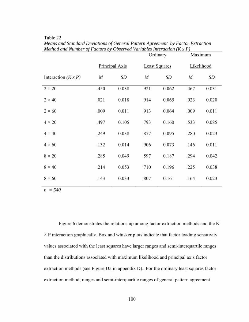
100
Table 22 Means and Standard Deviations of General Pattern Agreement by Factor Extraction Method and Number of Factors by Observed Variables Interaction (K x P)
Principal Axis
Ordinary
Least Squares
Maximum
Likelihood
Interaction (K x P) M SD M SD M SD
2 × 20 .450 0.038 .921 0.062 .467 0.031
2 × 40 .021 0.018 .914 0.065 .023 0.020
2 × 60 .009 0.011 .913 0.064 .009 0.011
4 × 20 .497 0.105 .793 0.160 .533 0.085
4 × 40 .249 0.038 .877 0.095 .280 0.023
4 × 60 .132 0.014 .906 0.073 .146 0.011
8 × 20 .285 0.049 .597 0.187 .294 0.042
8 × 40 .214 0.053 .710 0.196 .225 0.038
8 × 60 .143 0.033 .807 0.161 .164 0.023
n = 540
Figure 6 demonstrates the relationship among factor extraction methods and the K
× P interaction graphically. Box and whisker plots indicate that factor loading sensitivity
values associated with the least squares have larger ranges and semi-interquartile ranges
than the distributions associated with maximum likelihood and principal axis factor
extraction methods (see Figure D5 in appendix D). For the ordinary least squares factor
extraction method, ranges and semi-interquartile ranges of general pattern agreement
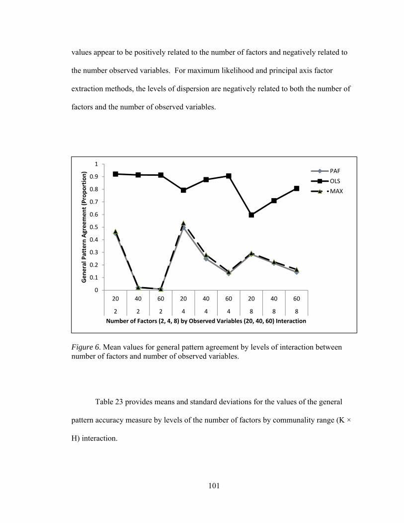
101
values appear to be positively related to the number of factors and negatively related to
the number observed variables. For maximum likelihood and principal axis factor
extraction methods, the levels of dispersion are negatively related to both the number of
factors and the number of observed variables.
Figure 6. Mean values for general pattern agreement by levels of interaction between number of factors and number of observed variables. Table 23 provides means and standard deviations for the values of the general
pattern accuracy measure by levels of the number of factors by communality range (K ×
H) interaction.
0
0.1
0.2
0.3
0.4
0.5
0.6
0.7
0.8
0.9
1
20 40 60 20 40 60 20 40 60
2 2 2 4 4 4 8 8 8
General Pattern Agreement (Proportion)
Number of Factors (2, 4, 8) by Observed Variables (20, 40, 60) Interaction
PAF
OLS
MAX
102
Table 23 Means and Standard Deviations of General Pattern Agreement for Factor Extraction Method and Number of Factors by Communality Range Interaction (K x H)
Principal Axis
Ordinary
Least Squares
Maximum
Likelihood
Interaction (K x H) M SD M SD M SD
2 × Low .153 0.186 .848 0.050 .166 0.201
2 × Wide .163 0.203 .922 0.030 .166 0.205
2 × High .164 0.233 .977 0.018 .167 0.239
4 × Low .242 0.118 .737 0.122 .288 0.126
4 × Wide .292 0.147 .868 0.062 .312 0.152
4 × High .344 0.206 .971 0.022 .359 0.210
8 × Low .170 0.048 .493 0.149 .195 0.045
8 × Wide .213 0.067 .727 0112 .223 0.054
8 × High .260 0.075 .894 0.068 .261 0.073
N = 540
Mean values for the general pattern accuracy are highest for ordinary least squares
across all levels of the interaction effect. In the case of ordinary least squares, the mean
values for the general pattern accuracy measure appear to be positively related to the
level of communality and negatively related to the number of factors; this general trend is
not apparent in mean values of general pattern agreement for principal axis and
maximum likelihood factor extraction methods. As the graphed means in Figure 7

103
indicate, the differences in mean levels of general pattern agreement are the smallest at
the four factors by high communality condition.
Figure 7. Mean values of general pattern agreement for levels of interaction between number of factors and communality.
For all levels of the number of factors by communality interaction, box and
whisker plots indicate that factor loading sensitivity values associated with the least
squares have smaller ranges and semi-interquartile ranges than the distributions
associated with maximum likelihood and principal axis factor extraction methods (see
Figure D6 in appendix D). For the ordinary least squares factor extraction method,
communality range in the distributions of general pattern agreement values appear to be
0
0.1
0.2
0.3
0.4
0.5
0.6
0.7
0.8
0.9
1
Low Wide High Low Wide High Low Wide High
2 2 2 4 4 4 8 8 8
Mean
General Pattern Agreement
Number of Factors by Communality Level Interaction
PAF
OLS
MAX

104
positively related to the number of factors and negatively related to the level of
communality. For maximum likelihood and principal axis factor extraction methods, the
levels of dispersion are negatively related to the number of factors and positively related
to the level of communality.
Table 24 provides means and standard deviations for the values of the general
pattern agreement measure by number of observed variables and communality range (P ×
H) interaction. The mean values for the general pattern agreement are highest for
Ordinary Least Squares across all levels of the interaction effect. In the case of ordinary
least squares, the mean values for the general pattern agreement appear to be positively
related to both number of observed variables and the level of communality. Principal
Axis Factor and Maximum Likelihood factor extractions yield similar mean values for
general pattern agreement across all levels of the P × H interaction. As the number of
observed variables increases, the mean values of general pattern agreement associated
with Ordinary Least Squares improves to a greater extent over the other two factor
extraction methods. These relationships are summarized graphically in Figure 8.
Box and whisker plots of general pattern agreement by levels of the P × H
interaction highlight several relationships among communality range, factor extraction
method, and level of interaction. In conditions that include 60 observed variables, several
outliers are present in distributions associated with the ordinary least squares factor
extraction method. In these distributions of general pattern agreement, ranges and semi-
interquartile ranges are negatively related to both number of observed variables and level
of communality.

105
Table 24 Means and Standard Deviations of General Pattern Agreement for Factor Extraction Method and Number of Observed Variables and Communality Range Interaction (P x H)
Principal Axis
Ordinary
Least Squares
Maximum
Likelihood
Interaction (P x H) M SD M SD M SD
20 × Low .343 0.343 .614 0.214 .383 0.097
20 × Wide .408 0.408 .780 0.143 .417 0.097
20 × High .481 0.481 .916 0.076 .493 0.125
40 × Low .134 0.134 .696 0.178 .162 0.099
40 × Wide .166 0.166 .850 0.091 .177 0.103
40 × High .185 0.184 .953 0.042 .189 0.138
60 × Low .088 0.088 .768 0.132 .107 0.063
60 × Wide .090 0.094 .885 0.056 .106 0.071
60 × High .100 0.101 .972 0.025 .106 0.080
N = 540
In distributions associated with maximum likelihood and principal axis factor
extraction methods, measures of dispersion are positively related to communality and
negatively related to the number of observed variables.

106
Figure 8. Mean values of general pattern agreement for levels of interaction between number of observed variables and communality.
Table 25 provides means and standard deviations for the values of the general
pattern agreement measure by levels of sample size by communality range (N × H)
interaction. The mean values for the general pattern accuracy measure are highest for
ordinary least squares across all levels of the interaction effect. In the case of ordinary
least squares, the mean values for the general pattern accuracy measure appear to be
positively related to both sample size and the level of communality; this general trend in
mean, general pattern agreement values is present in the principal axis and maximum
likelihood factor extraction method; however, the trend is less pronounced.
Box and whisker plots of general pattern agreement values indicate that semi-
interquartile ranges are negatively related to both communality level and sample size in
0
0.1
0.2
0.3
0.4
0.5
0.6
0.7
0.8
0.9
1
Low Wide High Low Wide High Low Wide High
20 20 20 40 40 40 60 60 60
Mean
General Pattern Agreement
Observed Variables by Communality Level Interaction
PAF
OLS
MAX
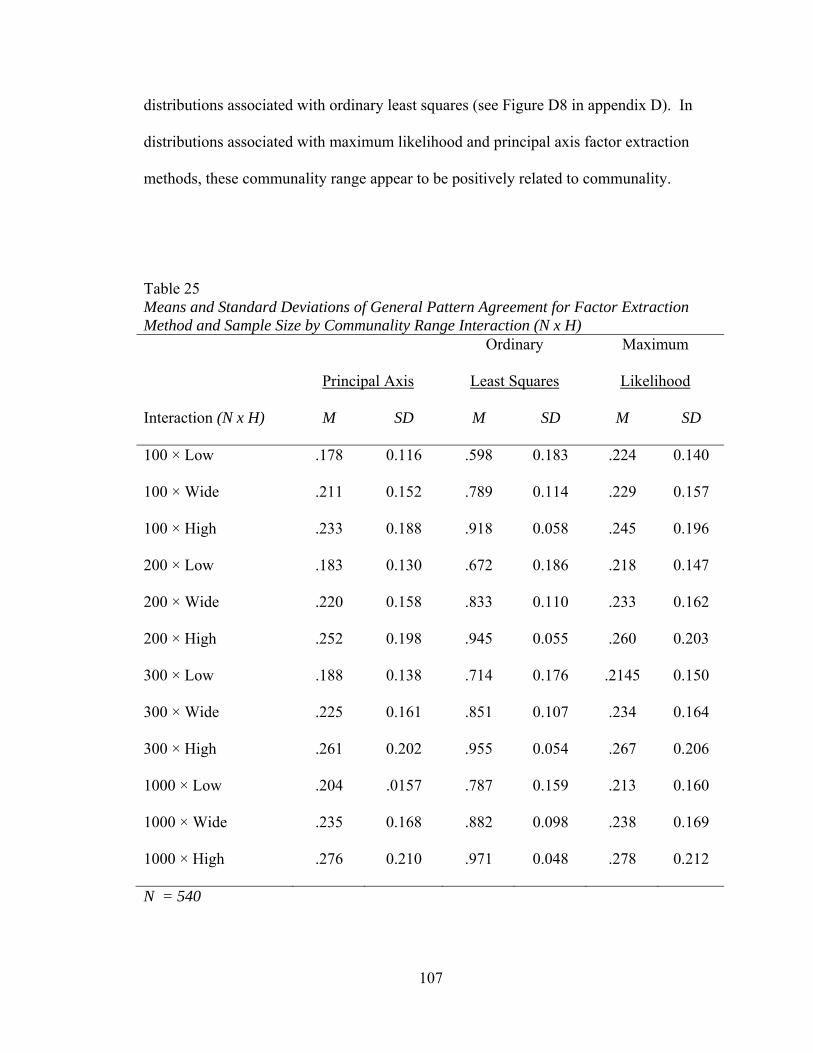
107
distributions associated with ordinary least squares (see Figure D8 in appendix D). In
distributions associated with maximum likelihood and principal axis factor extraction
methods, these communality range appear to be positively related to communality.
Table 25 Means and Standard Deviations of General Pattern Agreement for Factor Extraction Method and Sample Size by Communality Range Interaction (N x H)
Principal Axis
Ordinary
Least Squares
Maximum
Likelihood
Interaction (N x H) M SD M SD M SD
100 × Low .178 0.116 .598 0.183 .224 0.140
100 × Wide .211 0.152 .789 0.114 .229 0.157
100 × High .233 0.188 .918 0.058 .245 0.196
200 × Low .183 0.130 .672 0.186 .218 0.147
200 × Wide .220 0.158 .833 0.110 .233 0.162
200 × High .252 0.198 .945 0.055 .260 0.203
300 × Low .188 0.138 .714 0.176 .2145 0.150
300 × Wide .225 0.161 .851 0.107 .234 0.164
300 × High .261 0.202 .955 0.054 .267 0.206
1000 × Low .204 .0157 .787 0.159 .213 0.160
1000 × Wide .235 0.168 .882 0.098 .238 0.169
1000 × High .276 0.210 .971 0.048 .278 0.212
N = 540
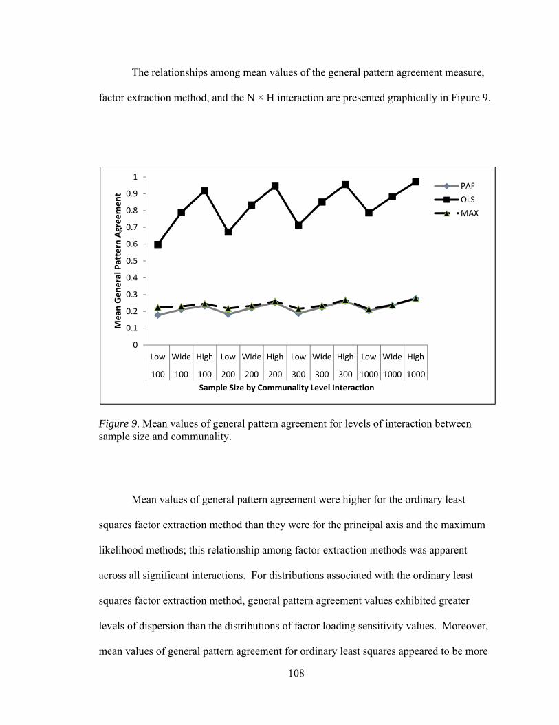
108
The relationships among mean values of the general pattern agreement measure,
factor extraction method, and the N × H interaction are presented graphically in Figure 9.
Figure 9. Mean values of general pattern agreement for levels of interaction between sample size and communality.
Mean values of general pattern agreement were higher for the ordinary least
squares factor extraction method than they were for the principal axis and the maximum
likelihood methods; this relationship among factor extraction methods was apparent
across all significant interactions. For distributions associated with the ordinary least
squares factor extraction method, general pattern agreement values exhibited greater
levels of dispersion than the distributions of factor loading sensitivity values. Moreover,
mean values of general pattern agreement for ordinary least squares appeared to be more
0
0.1
0.2
0.3
0.4
0.5
0.6
0.7
0.8
0.9
1
Low Wide High Low Wide High Low Wide High Low Wide High
100 100 100 200 200 200 300 300 300 1000 1000 1000
Mean
General Pattern Agreement
Sample Size by Communality Level Interaction
PAF
OLS
MAX

109
closely related to the values of the interaction effects than was the case with factor
loading sensitivity.
Per Element Pattern Agreement
The measure for per element pattern agreement is based on a P × K matrix.
Elements of each matrix contained ones, indicating agreement, where the corresponding
factor loading had an absolute value of .30 or greater in both the sample and population
factor pattern matrices; elements of the matrix also contained ones when the variable had
loadings of less than the absolute value of .30 on the corresponding factor in both the
sample and population. When these criteria are not met, the element had a value of zero.
The resulting measure of per element pattern agreement is the proportion of samples in
which the agreement criteria were met for each observed variable by factor combination.
Table 26 presents descriptive statistics concerning the distribution of the per element
pattern agreement measure by each of the tested factor extraction methods.
Shapiro-Wilks’ tests of normality for per element pattern agreement measures
associated with all three factor extraction methods yield evidence that the three
distributions do not conform to assumptions regarding univariate normality. Mauchly’s
test of transformed variables, (2) = 494.79, p < .0001, indicate that the data do not
conform to the sphericity assumption associated with repeated measures ANOVA. To
address the potential for increased Type I error rate, tests of significance associated with
the repeated measures analysis of variance will be based on the Greenhouse-Geisser
adjustment to degrees of freedom (Stevens, 2002).

110
Table 26 Descriptive Statistics for Distribution of Per Element Pattern Agreement Values Factor Extraction Method N M SD Skewness Kurtosis
Principal Axis 540 .593 0.180 -0.842 -0.465
Ordinary Least Squares 540 .750 0.750 0.005 -0.819
Maximum Likelihood 540 .605 0.185 -0.892 -0.445
The results of the multivariate analyses of variance indicate that per element
agreement differed significantly by factor extraction method, Λ .008,F 2, 459) =
26828.4, p <.0001. In addition to the method main effect, per element agreement values
differed significantly by all main effects. The multivariate analysis of variance indicated
that per element agreement differed significantly across eight of the first-order
interactions. The results of this analysis are presented in Table C4 (see Appendix C).
The univariate, repeated measures analysis of variance also indicated that per
element pattern agreement differed significantly based on factor extraction method, F(2,
920) = 45801.9, p< .0001, = .934. Results of the between subject portion of the
analysis indicated that all manipulated research characteristics, main effects, were
associated with significant differences in per element pattern agreement. Moreover, per
element pattern agreement differed significantly by all interactions between factor
extraction method and main effects. The model that included main effects and first-
order interactions among main effects accounted for 98.7% of the variability in the
observed data (see Table C6 in appendix C).

111
The between and within sections of the univariate, repeated measures analysis
identified number of factors by observed variables (K × P), number of factors by sample
size (K × N), number of factors by level of communality (K × H), number of factors by
level of dichotomization (K × D), number of observed variables by level of communality
(P × H), number of observed variables by level of dichotomization (P × D), sample size
by communality (N × H), and level of communality by level of dichotomization (H × D)
as sources of significant differences in per element pattern agreement. In the between
groups analysis, per element agreement differed significantly by levels of the interaction
between number of variables and sample size (P × N), F (6, 460) = 4.16, p = .0004, =
.044; however, when factor extraction method is included, the within groups analysis, this
significant effect is not present. From both perspectives, the sources of variation that
included the P × N interaction failed to yield a medium effect size (Cohen, 1988).
According to the results of within subjects analyses, the number of factors by
observed variables, F (8, 920) = 724.05, p < .0001, = .474, and the samples size by
communality range, F (12, 920) = 44.65, p < .0001 , = .077, were both statistically
significant and yielded effect sizes that were medium or greater. The betweens subjects
analysis indicated that the following interactions met the criteria for continued analyses:
1. Number of factors by sample size, F (6, 460) = 18.540, p< .0001, = .172
2. Number of factors by communality range, F (4, 460) = 96.70, p < .0001, =
.419
3. Number of observed variables by communality range, F (4, 460) = 25.54, p <
.0001, = .155.
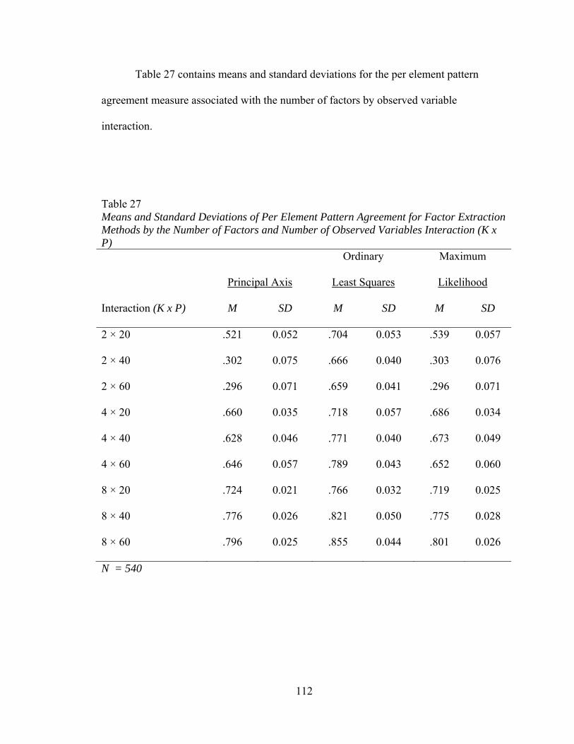
112
Table 27 contains means and standard deviations for the per element pattern
agreement measure associated with the number of factors by observed variable
interaction.
Table 27 Means and Standard Deviations of Per Element Pattern Agreement for Factor Extraction Methods by the Number of Factors and Number of Observed Variables Interaction (K x P)
Principal Axis
Ordinary
Least Squares
Maximum
Likelihood
Interaction (K x P) M SD M SD M SD
2 × 20 .521 0.052 .704 0.053 .539 0.057
2 × 40 .302 0.075 .666 0.040 .303 0.076
2 × 60 .296 0.071 .659 0.041 .296 0.071
4 × 20 .660 0.035 .718 0.057 .686 0.034
4 × 40 .628 0.046 .771 0.040 .673 0.049
4 × 60 .646 0.057 .789 0.043 .652 0.060
8 × 20 .724 0.021 .766 0.032 .719 0.025
8 × 40 .776 0.026 .821 0.050 .775 0.028
8 × 60 .796 0.025 .855 0.044 .801 0.026
N = 540
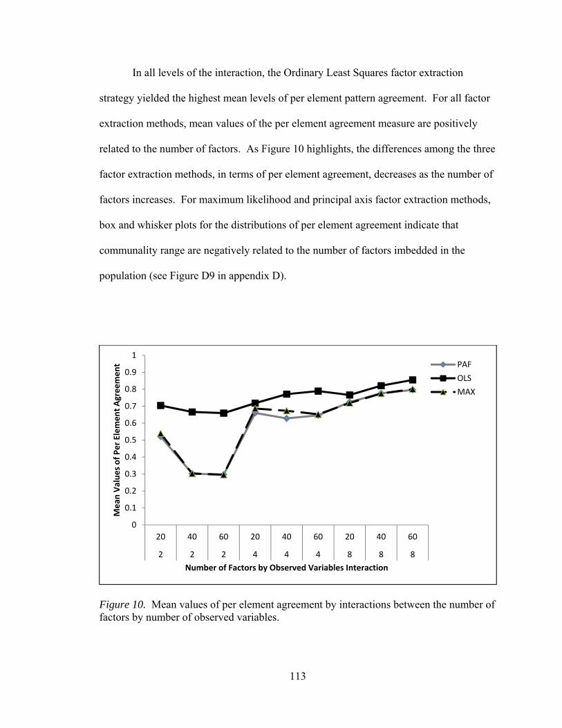
113
In all levels of the interaction, the Ordinary Least Squares factor extraction
strategy yielded the highest mean levels of per element pattern agreement. For all factor
extraction methods, mean values of the per element agreement measure are positively
related to the number of factors. As Figure 10 highlights, the differences among the three
factor extraction methods, in terms of per element agreement, decreases as the number of
factors increases. For maximum likelihood and principal axis factor extraction methods,
box and whisker plots for the distributions of per element agreement indicate that
communality range are negatively related to the number of factors imbedded in the
population (see Figure D9 in appendix D).
Figure 10. Mean values of per element agreement by interactions between the number of factors by number of observed variables.
0
0.1
0.2
0.3
0.4
0.5
0.6
0.7
0.8
0.9
1
20 40 60 20 40 60 20 40 60
2 2 2 4 4 4 8 8 8
Mean
Values of Per Element Agreement
Number of Factors by Observed Variables Interaction
PAF
OLS
MAX

114
Table 28 presents means and standard deviations in per element accuracy for
levels of the number of factors by sample size interaction.
Table 28 Means and Standard Deviations of Per Element Agreement by Factor Extraction Method and Number of Factors by Sample Size Interaction (K x N)
Principal Axis
Ordinary
Least Squares
Maximum
Likelihood
Interaction (K x N) M SD M SD M SD
2 × 100 .375 0.112 .654 0.037 .388 0.128
2 × 200 .373 0.123 .675 0.044 .380 0.132
2 × 300 .372 0.128 .683 0.048 .377 0.134
2 × 1000 .371 0.137 .694 0.057 .372 0.138
4 × 100 .631 0.038 .712 0.052 .654 0.042
4 × 200 .652 0.042 .756 0.046 .669 0.048
4 × 300 .660 0.045 .772 0.043 .675 0.051
4 × 1000 .675 0.052 .798 0.045 .683 0.056
8 × 100 .731 0.041 .760 0.043 .743 0.039
8 × 200 .750 0.047 .808 0.044 .763 0.042
8 × 300 .758 0.048 .829 0.043 .770 0.043
8 × 1000 .770 0.047 .860 0.042 .782 0.041
N = 540
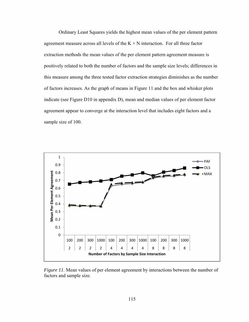
115
Ordinary Least Squares yields the highest mean values of the per element pattern
agreement measure across all levels of the K × N interaction. For all three factor
extraction methods the mean values of the per element pattern agreement measure is
positively related to both the number of factors and the sample size levels; differences in
this measure among the three tested factor extraction strategies diminishes as the number
of factors increases. As the graph of means in Figure 11 and the box and whisker plots
indicate (see Figure D10 in appendix D), mean and median values of per element factor
agreement appear to converge at the interaction level that includes eight factors and a
sample size of 100.
Figure 11. Mean values of per element agreement by interactions between the number of factors and sample size.
0
0.1
0.2
0.3
0.4
0.5
0.6
0.7
0.8
0.9
1
100 200 300 1000 100 200 300 1000 100 200 300 1000
2 2 2 2 4 4 4 4 8 8 8 8
Mean
Per Element Agreement
Number of Factors by Sample Size Interaction
PAF
OLS
MAX

116
Table 29 provides means and standard deviations for these values of per element
agreement for the number factors by level of communality (K × H) interaction. The
mean per element pattern agreement is highest for Ordinary Least Squares in all levels of
the interaction. The mean values for per element pattern agreement are positively related
to the number of factors and negatively related to the communality range.
Table 29 Means and Standard Deviations of Per Element Pattern Agreement for Factor Extraction Method and Number of Factors by Communality Range Interaction (K x H)
Principal Axis
Ordinary
Least Squares
Maximum
Likelihood
Interaction (K x H) M SD M SD M SD
2 × Low .444 0.092 .690 0.053 .456 0.107
2 × Wide .379 0.108 .690 0.047 .382 0.111
2 × High .296 0.125 .648 0.033 .300 0.130
4 × Low .697 0.032 .775 0.075 .721 0.021
4 × Wide .654 0.022 .758 0.047 .667 0.021
4 × High .612 0.040 .745 0.033 .622 0.042
8 × Low .775 0.047 .797 0.065 .792 0.038
8 × Wide .750 0.043 .815 0.054 .761 0.038
8 × High .732 0.044 .830 0.043 .741 0.038
N = 540

117
As the graph of means in Figure 12 and box an whisker plots (See Figure D11 in
appendix D) demonstrate, the relationship between per element pattern agreement and the
K × H interaction appears to be more pronounced in the principal axis and the maximum
likelihood factor extraction methods than in the ordinary least squares method.
Differences in mean per element agreement diminishes as the number of factors
increases; however, because of the negative relationship between levels communality and
per element agreement that is present in the principal axis and maximum likelihood factor
extraction methods, the smallest difference among the three factor extraction methods
occurs at the eights factors by low communality condition.
Figure 12. Mean values of per element agreement by interactions between the number of factors and communality.
0
0.1
0.2
0.3
0.4
0.5
0.6
0.7
0.8
0.9
1
Low Wide High Low Wide High Low Wide High
2 2 2 4 4 4 8 8 8
Mean
Per Element Agreement
Number of Factors by Communality Level Interaction
PAF
OLS
MAX
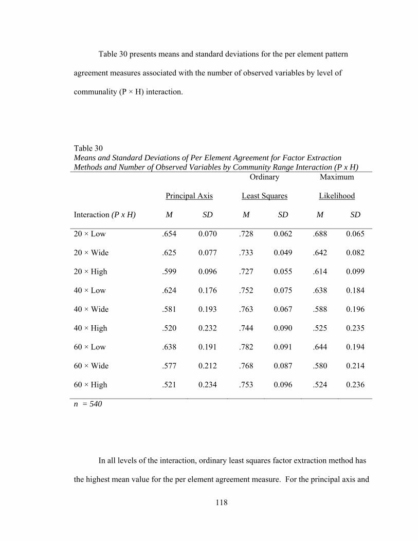
118
Table 30 presents means and standard deviations for the per element pattern
agreement measures associated with the number of observed variables by level of
communality (P × H) interaction.
Table 30 Means and Standard Deviations of Per Element Agreement for Factor Extraction Methods and Number of Observed Variables by Community Range Interaction (P x H)
Principal Axis
Ordinary
Least Squares
Maximum
Likelihood
Interaction (P x H) M SD M SD M SD
20 × Low .654 0.070 .728 0.062 .688 0.065
20 × Wide .625 0.077 .733 0.049 .642 0.082
20 × High .599 0.096 .727 0.055 .614 0.099
40 × Low .624 0.176 .752 0.075 .638 0.184
40 × Wide .581 0.193 .763 0.067 .588 0.196
40 × High .520 0.232 .744 0.090 .525 0.235
60 × Low .638 0.191 .782 0.091 .644 0.194
60 × Wide .577 0.212 .768 0.087 .580 0.214
60 × High .521 0.234 .753 0.096 .524 0.236
n = 540
In all levels of the interaction, ordinary least squares factor extraction method has
the highest mean value for the per element agreement measure. For the principal axis and

119
the maximum likelihood factor extraction methods, the relationship between per element
agreement and level of communality is negative. As the Figure 13 highlights, a negative
relationship between per element agreement and the number of observed variables also
exists for the principal axis and maximum likelihood factor extraction methods. The
negative relationship between the manipulated research conditions and per element
agreement is not associated with the ordinary least squares method.
Figure 13. Mean values of per element agreement by interactions between the number of observed variables and communality.
The patterns of central tendency and dispersion in distributions of per element
agreement for maximum likelihood and principal axis factor extraction methods are quite
0
0.1
0.2
0.3
0.4
0.5
0.6
0.7
0.8
0.9
1
Low Wide High Low Wide High Low Wide High
20 20 20 40 40 40 60 60 60
Mean
Per Element Agreement
Observed Variables by Communality Level Interaction
PAF
OLS
MAX

120
nearly identical (see Figure D12 in appendix D). While the generally negative
relationship between median and mean values of per element agreement and the level of
communality is present in all factor extraction methods, the pattern is not as strongly
expressed in distributions associated with ordinary least squares. In all conditions,
ordinary least squares factor extraction method yields distributions that have smaller
ranges and semi-interquartile ranges.
The mean values of per element pattern agreement associated with the sample size
by communality interaction (N × H) are presented in Table 31. For all levels of the
interaction, ordinary least squares yields the highest values of the per element factor
agreement measure. For all factor extraction methods, the relationship between sample
size and per element agreement is positive. For maximum likelihood and principal axis
factor extraction methods, the relationship between per element agreement and
communality is negative.
Figure 14 highlights the relationship among mean values of per element pattern
agreement measures, factor extraction methods, and levels of the N × H interaction. For
maximum likelihood and principal axis factor extraction methods, box and whisker plots
in Figure D13 (see appendix D) indicate that major changes in median, mean and semi-
interquartile range occur within the sample size conditions as opposed to across them; the
ranges in per element agreement increase as communality ranges from low through wide
to high. These patterns are not apparent in distributions associated with the ordinary least
squares factor extraction method.

121
Table 31 Means and Standard Deviations of Per Element Agreement for Factor Extraction Method and Sample Size by Communality Range Interaction (N x H)
Principal Axis
Ordinary
Least Squares
Maximum
Likelihood
Interaction (N x H) M SD M SD M SD
100 × Low .619 0.140 .687 0.054 .644 0.144
100 × Wide .581 0.160 .717 0.057 .594 0.164
100 × High .537 0.189 .722 0.069 .547 0.192
200 × Low .636 0.153 .745 0.066 .656 0.159
200 × Wide .593 0.171 .752 0.066 .603 0.176
200 × High .546 0.201 .741 0.081 .554 0.204
300 × Low .643 0.159 .772 0.069 .660 0.164
300 × Wide .598 0.176 .766 0.070 .606 0.180
300 × High .549 0.205 .747 0.086 .556 0.209
1000 × Low .657 0.169 .812 0.074 .664 0.173.
1000 × Wide .605 0.184 .784 0.076 .611 0.187
1000 × High .554 0.213 .755 0.093 .559 0.216
N = 540

122
Figure 14. Mean values of per element agreement by interactions between sample size and communality.
Across all interactions among main effects, mean per element agreement values
for the ordinary least squares factor extraction exceeded the mean values associated with
principal axis and maximum likelihood methods. For interactions that included the
number of factors imbedded in the population main effect, the differences among the
three factor extraction methods, in terms of mean per element agreement, diminished as
the number of factors increased. In all interactions that included communality, the
relationship between mean per element agreement values and communality was negative;
this relationship was apparent for all factor extraction methods.
Total Pattern Agreement
Total pattern agreement is measured through a scalar. This scalar is populated
with a one when the mean of the per element agreement matrix is one. If any element of
0
0.1
0.2
0.3
0.4
0.5
0.6
0.7
0.8
0.9
1
Low Wide High Low Wide High Low Wide High Low Wide High
100 100 100 200 200 200 300 300 300 1000 1000 1000
Mean
Per Element Agreement
Sample Size by Communality Level Interaction
PAF
OLS
MAX
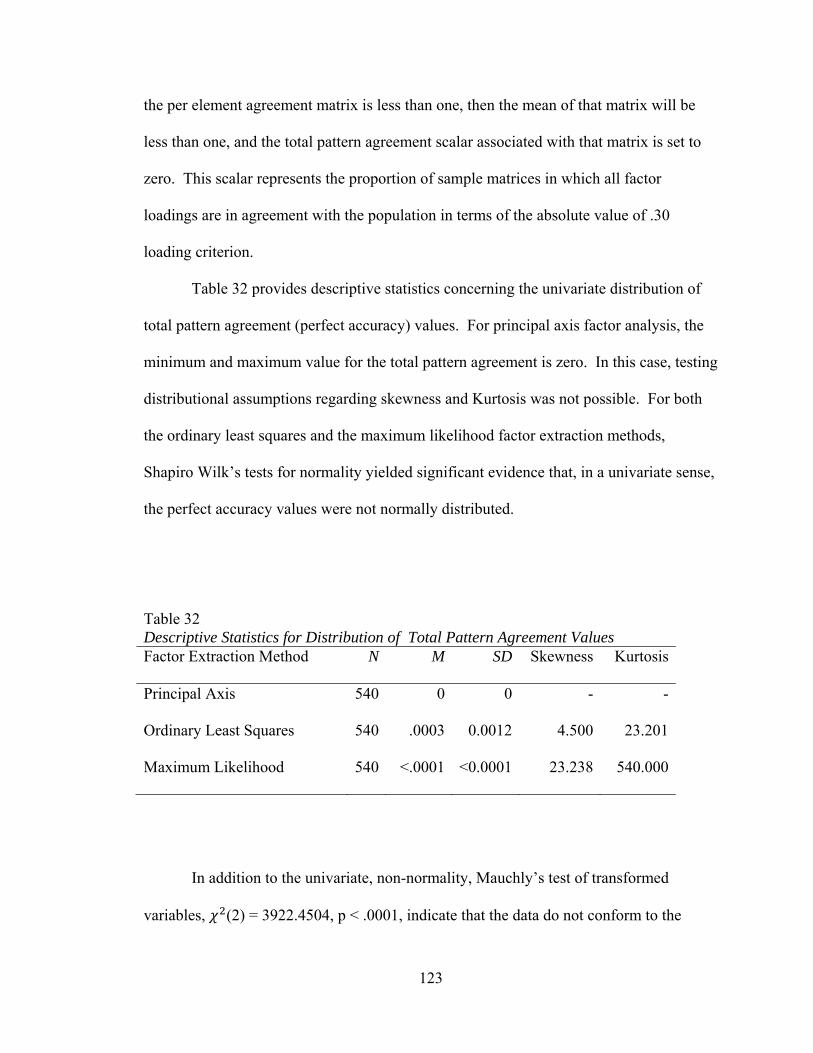
123
the per element agreement matrix is less than one, then the mean of that matrix will be
less than one, and the total pattern agreement scalar associated with that matrix is set to
zero. This scalar represents the proportion of sample matrices in which all factor
loadings are in agreement with the population in terms of the absolute value of .30
loading criterion.
Table 32 provides descriptive statistics concerning the univariate distribution of
total pattern agreement (perfect accuracy) values. For principal axis factor analysis, the
minimum and maximum value for the total pattern agreement is zero. In this case, testing
distributional assumptions regarding skewness and Kurtosis was not possible. For both
the ordinary least squares and the maximum likelihood factor extraction methods,
Shapiro Wilk’s tests for normality yielded significant evidence that, in a univariate sense,
the perfect accuracy values were not normally distributed.
Table 32 Descriptive Statistics for Distribution of Total Pattern Agreement Values Factor Extraction Method N M SD Skewness Kurtosis
Principal Axis 540 0 0 - -
Ordinary Least Squares 540 .0003 0.0012 4.500 23.201
Maximum Likelihood 540 <.0001 <0.0001 23.238 540.000
In addition to the univariate, non-normality, Mauchly’s test of transformed
variables, (2) = 3922.4504, p < .0001, indicate that the data do not conform to the
124
sphericity assumption associated with repeated measures ANOVA. The results of the
multivariate analyses of variance indicate that total pattern agreement differs significantly
by factor extraction method, Λ .7920,F 2, 459) = 85.36, p <.0001. In addition to the
method main effect, total pattern accuracy differed significantly by interactions between
factor extraction method and the number of factors, observed variables, sample size, and
level of dichotomization. However, the mean values of total pattern agreement were not
substantially greater than zero in any of the studied conditions. While statistically
significant differences among means were found, comparisons among zero values were
not informative and are not included in this study.
Congruence
The congruence among factor pattern matrices simulated in the population and the
sample pattern matrices is measured through a congruence coefficient. As defined by
MaCallum (et al., 1999), the phi coefficient is the cosine of the angle between the sample
and population factor solutions “when plotted on the same space” (p. 93). To assess the
congruence across all factor loading matrices, an average of the phi coefficient was
calculated for each factor extraction method. Table 33 provides descriptive statistics
concerning the univariate distribution of the mean phi coefficients (Congruence) for each
of the tested factor extraction methods.
Shapiro-Wilks’ tests of normality for mean congruence associated with all three
factor extraction methods yield evidence that the three distributions do not conform to the
assumptions of univariate normality. Mauchly’s test of transformed variables (2) =
989.341, p < .0001, indicate that the data do not conform to the sphericity assumption
associated with repeated measures ANOVA. To address the potential for increased Type

125
I error rate, tests of significance associated with the repeated measures analysis of
variance will be based on the Greenhouse-Geisser adjustment to degrees of freedom
(Stevens, 2002).
Table 33 Descriptive Statistics for Distribution of Congruence Factor Extraction Method N M SD Skewness Kurtosis
Principal Axis 540 .454 0.240 -0.230 -1.312
Ordinary Least Squares 540 .496 0.215 -0.219 -1.274
Maximum Likelihood 540 0.556 0.236 -0.487 -1.166
Results of the multivariate analysis of variance indicate that the factor extraction
method yield significant differences in mean values of congruence, Λ = .0262, F (2, 459)
= 8533.92, p < .0001. In addition to the method main effect, all of the manipulated
research characteristics yielded significantly different congruence levels (see Table C9 in
appendix C). The univariate, repeated measures analysis of variance also indicates that
level of congruence between sample and population loading matrices differ significantly
by factor extraction method, F(2, 920) = 7026.19, p < .0001, = .966 (see Table C 10 in
appendix C). The model including main effects and first-order interactions accounted for
97.1% of the variability associated with the measure of congruence between population
and sample factor pattern matrices.
As results of the between subjects analyses indicate, all main effects and six of the
ten first-order interaction effects are associated with significant differences among
126
congruence values; the significant interaction effects include number of factors by
observed variables (K × P), number of factors by sample size (K × N), number of factors
by communality range (K × H), number of factors by dichotomization level (K × D),
sample size by level of communality (N × H), and level of communality by level of
dichotomization (H × D) . Results of the within subjects analysis indicate that the
interactions of factor extraction methods with the number of factors, number of observed
variables, sample size, and level of communality are associated with significant
differences in congruence between sample and population factor loading matrices. The
level of dichotomization does not yield significant results.
In addition to yielding statistically significant differences in average congruence
between population and sample factor pattern matrices, the between subjects analyses
yielded at least medium effect sizes for the following interactions:
1. Number of factors by observed variables, F(4, 460) = 85.49, p < .0001, =
.405
2. Number of factors by sample size, F(6, 460) = 10.89, pr < .0001, = .115
3. Number of factors by level of dichotomization, F(8, 460) = 5.94, p < .0001,
= .086
4. Sample size by level of communality, F(6, 460) = 7.46, p < .0001, = .067
5. Level of communality by dichotomization, F(8, 460) = 5.17, p < .0001, =
.076
Comparisons among means were conducted for these interactions only.
Table 34 presents means and standard deviations for the mean congruence
measure associated with the number of factors by observed variable interaction.

127
Table 34 Means and Standard Deviations of Congruence Values for Factor Extraction Method and Number of Factors by Observed Variables Interaction (K x P)
Principal Axis
Ordinary
Least Squares
Maximum
Likelihood
Interaction (K x P) M SD M SD M SD
2 × 20 .712 0.093 .728 0.082 .789 0.079
2 × 40 .690 0.073 .710 0.069 .784 0.040
2 × 60 .692 0.076 .711 0.072 .784 0.045
4 × 20 .409 0.119 .460 0.104 .522 0.094
4 × 40 .513 0.092 .540 0.081 .638 0.050
4 × 60 .573 0.084 .596 0.075 .690 0.049
8 × 20 .088 0.022 .171 0.033 .179 0.054
8 × 40 .172 0.067 .249 0.064 .264 0.095
8 × 60 .242 0.090 .303 0.083 .351 0.104
N = 540
Across all interactions between the number of factors and observed variables,
maximum likelihood factor extraction yielded higher mean levels of congruence between
sample and population factor pattern matrices. The smallest, mean congruence values are
associated with principal axis factor analysis. The graph of means in Figure 15 highlights
the negative relationship among mean phi values and the number of factors.
As box and whisker plots indicate, ranges and semi-interquartile ranges for values
of congruence decrease as the number of factors increase (see Figure D17 in appendix

128
D). However, in the eight factor conditions for all three factor extraction methods, these
semi-interquartile ranges increase in value as the number of observed variables increase.
In the two and four factor conditions, the semi-interquartile range decreases as the
number of observed variables increase.
Figure 15. Mean values of congruence by interactions between the number of factors and number observed variables.
Means and standard deviations for congruence by interactions among the number
of factors and sample size are presented in Table 35.
0
0.1
0.2
0.3
0.4
0.5
0.6
0.7
0.8
0.9
1
20 40 60 20 40 60 20 40 60
2 2 2 4 4 4 8 8 8
Average
Coefficient of Congruence
Number of Factors by Observed Variables Interaction
PAF
OLS
MAX

129
Table 35 Means and Standard Deviations of Congruence Values for Factor Extraction Method and Number of Factors by Sample Size Interaction (K x N)
Principal Axis
Ordinary
Least Squares
Maximum
Likelihood
Interaction (K x N) M SD M SD M SD
2 × 100 .636 0.068 .659 0.063 .783 0.050
2 × 200 .689 0.070 .708 0.064 .786 0.056
2 × 300 .712 0.070 .729 0.064 .787 0.058
2 × 1000 .755 0.071 .768 .065 .788 0.065
4 × 100 .392 0.099 .439 0.086 .557 0.110
4 × 200 .477 0.098 .514 0.083 .612 0.090
4 × 300 .519 0.094 .550 0.080 .632 0.082
4 × 1000 .605 0.081 .625 0.067 .664 0.073
8× 100 .113 0.046 .187 0.049 .165 0.052
8 × 200 .150 0.069 .225 0.063 .241 0.078
8 × 300 .172 0.081 .247 0.072 .281 0.090
8 × 1000 .234 0.110 .305 0.097 .370 0.106
N = 540
The values indicate that the mean congruence values decreases as the number of
factors increase. In general, the level of congruence increases as the sample size
increases for all three factor extraction methods. With the exception of the eight-factor
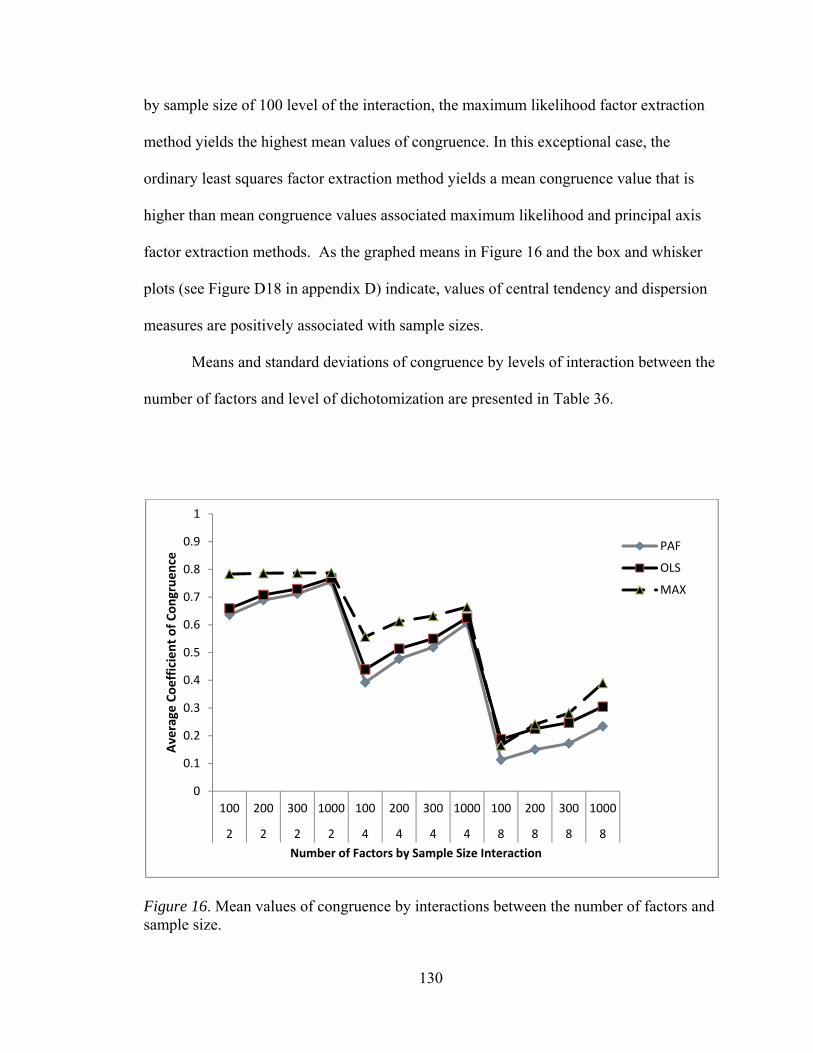
130
by sample size of 100 level of the interaction, the maximum likelihood factor extraction
method yields the highest mean values of congruence. In this exceptional case, the
ordinary least squares factor extraction method yields a mean congruence value that is
higher than mean congruence values associated maximum likelihood and principal axis
factor extraction methods. As the graphed means in Figure 16 and the box and whisker
plots (see Figure D18 in appendix D) indicate, values of central tendency and dispersion
measures are positively associated with sample sizes.
Means and standard deviations of congruence by levels of interaction between the
number of factors and level of dichotomization are presented in Table 36.
Figure 16. Mean values of congruence by interactions between the number of factors and sample size.
0
0.1
0.2
0.3
0.4
0.5
0.6
0.7
0.8
0.9
1
100 200 300 1000 100 200 300 1000 100 200 300 1000
2 2 2 2 4 4 4 4 8 8 8 8
Average
Coefficient of Congruence
Number of Factors by Sample Size Interaction
PAF
OLS
MAX
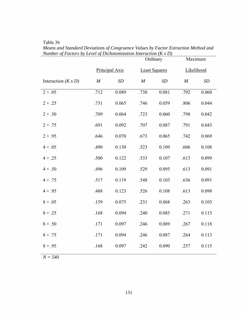
131
Table 36 Means and Standard Deviations of Congruence Values by Factor Extraction Method and Number of Factors by Level of Dichotomization Interaction (K x D)
Principal Axis
Ordinary
Least Squares
Maximum
Likelihood
Interaction (K x D) M SD M SD M SD
2 × .05 .712 0.089 .730 0.081 .792 0.060
2 × .25 .731 0.065 .746 0.059 .806 0.044
2 × .50 .709 0.064 .723 0.060 .798 0.042
2 × .75 .691 0.092 .707 0.087 .791 0.043
2 × .95 .646 0.070 .673 0.065 .742 0.069
4 × .05 .490 0.130 .523 0.109 .606 0.108
4 × .25 .500 0.122 .533 0.107 .613 0.099
4 × .50 .496 0.109 .529 0.095 .613 0.091
4 × .75 .517 0.119 .548 0.103 .636 0.091
4 × .95 .488 0.123 .526 0.108 .613 0.098
8 × .05 .159 0.075 .231 0.068 .263 0.103
8 × .25 .168 0.094 .240 0.085 .271 0.115
8 × .50 .171 0.097 .246 0.089 .267 0.118
8 × .75 .171 0.094 .246 0.087 .264 0.113
8 × .95 .168 0.097 .242 0.090 .257 0.115
N = 540
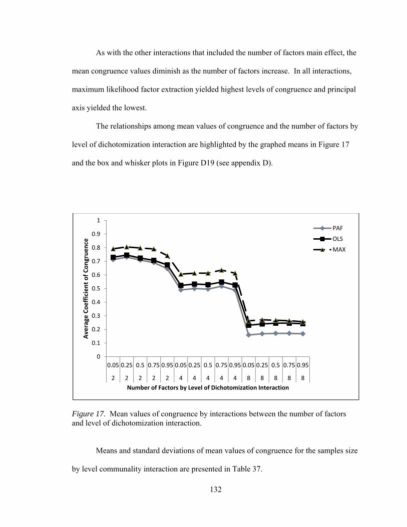
132
As with the other interactions that included the number of factors main effect, the
mean congruence values diminish as the number of factors increase. In all interactions,
maximum likelihood factor extraction yielded highest levels of congruence and principal
axis yielded the lowest.
The relationships among mean values of congruence and the number of factors by
level of dichotomization interaction are highlighted by the graphed means in Figure 17
and the box and whisker plots in Figure D19 (see appendix D).
Figure 17. Mean values of congruence by interactions between the number of factors and level of dichotomization interaction.
Means and standard deviations of mean values of congruence for the samples size
by level communality interaction are presented in Table 37.
0
0.1
0.2
0.3
0.4
0.5
0.6
0.7
0.8
0.9
1
0.05 0.25 0.5 0.75 0.95 0.05 0.25 0.5 0.75 0.95 0.05 0.25 0.5 0.75 0.95
2 2 2 2 2 4 4 4 4 4 8 8 8 8 8
Average
Coefficient of Congruence
Number of Factors by Level of Dichotomization Interaction
PAF
OLS
MAX
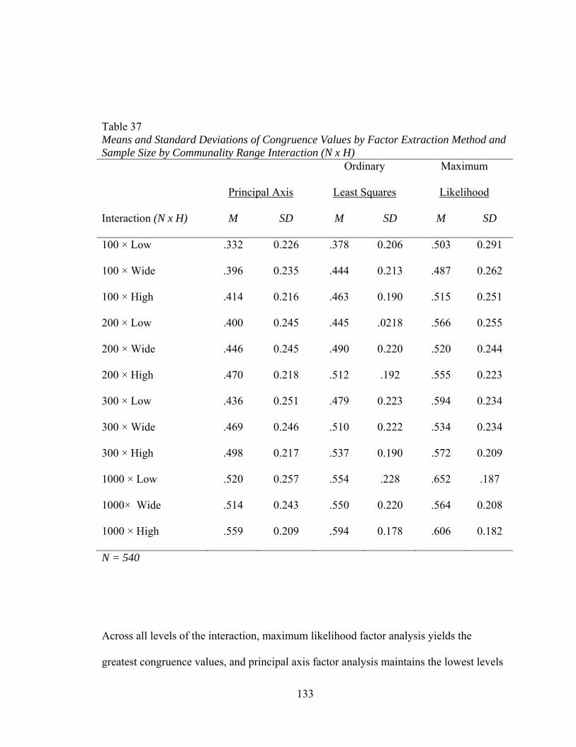
133
Table 37 Means and Standard Deviations of Congruence Values by Factor Extraction Method and Sample Size by Communality Range Interaction (N x H)
Principal Axis
Ordinary
Least Squares
Maximum
Likelihood
Interaction (N x H) M SD M SD M SD
100 × Low .332 0.226 .378 0.206 .503 0.291
100 × Wide .396 0.235 .444 0.213 .487 0.262
100 × High .414 0.216 .463 0.190 .515 0.251
200 × Low .400 0.245 .445 .0218 .566 0.255
200 × Wide .446 0.245 .490 0.220 .520 0.244
200 × High .470 0.218 .512 .192 .555 0.223
300 × Low .436 0.251 .479 0.223 .594 0.234
300 × Wide .469 0.246 .510 0.222 .534 0.234
300 × High .498 0.217 .537 0.190 .572 0.209
1000 × Low .520 0.257 .554 .228 .652 .187
1000× Wide .514 0.243 .550 0.220 .564 0.208
1000 × High .559 0.209 .594 0.178 .606 0.182
N = 540
Across all levels of the interaction, maximum likelihood factor analysis yields the
greatest congruence values, and principal axis factor analysis maintains the lowest levels
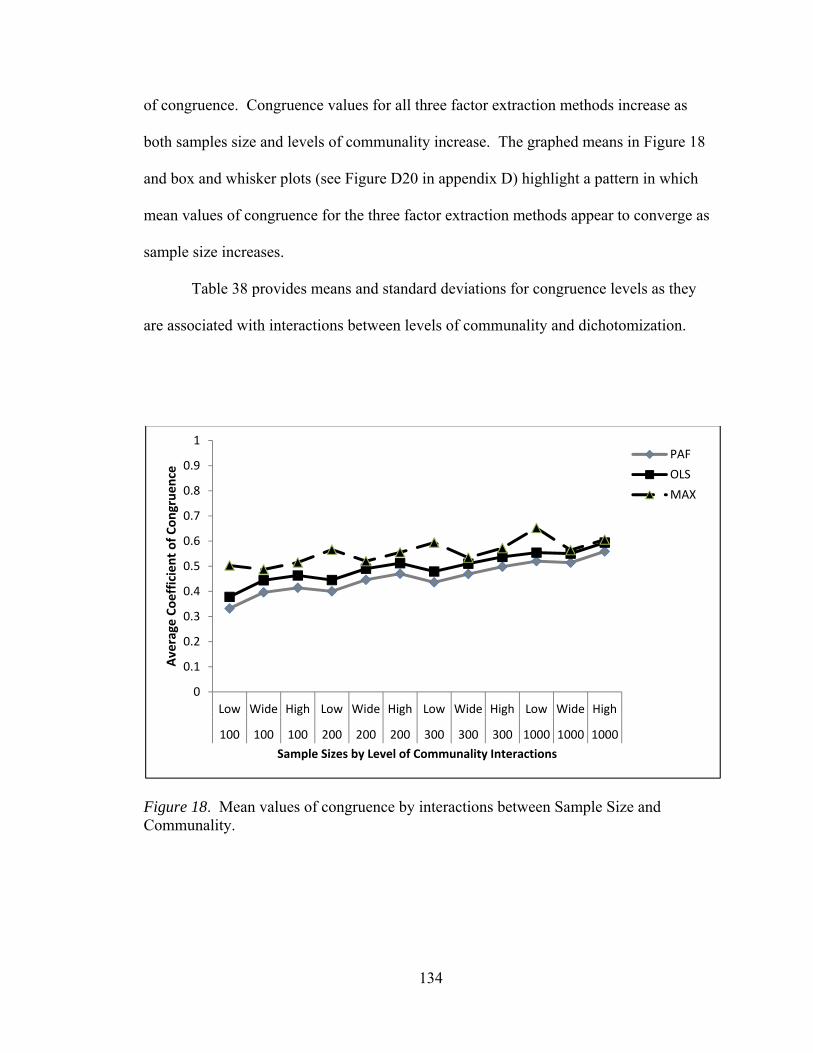
134
of congruence. Congruence values for all three factor extraction methods increase as
both samples size and levels of communality increase. The graphed means in Figure 18
and box and whisker plots (see Figure D20 in appendix D) highlight a pattern in which
mean values of congruence for the three factor extraction methods appear to converge as
sample size increases.
Table 38 provides means and standard deviations for congruence levels as they
are associated with interactions between levels of communality and dichotomization.
Figure 18. Mean values of congruence by interactions between Sample Size and Communality.
0
0.1
0.2
0.3
0.4
0.5
0.6
0.7
0.8
0.9
1
Low Wide High Low Wide High Low Wide High Low Wide High
100 100 100 200 200 200 300 300 300 1000 1000 1000
Average
Coefficient of Congruence
Sample Sizes by Level of Communality Interactions
PAF
OLS
MAX
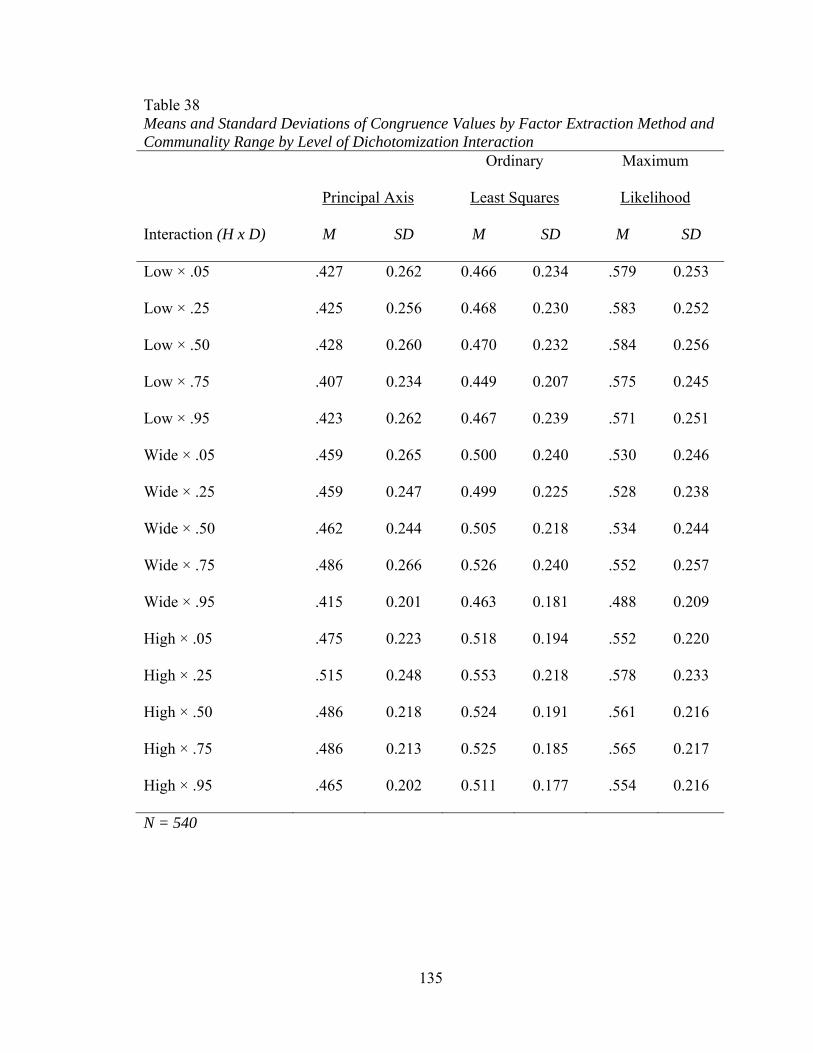
135
Table 38 Means and Standard Deviations of Congruence Values by Factor Extraction Method and Communality Range by Level of Dichotomization Interaction
Principal Axis
Ordinary
Least Squares
Maximum
Likelihood
Interaction (H x D) M SD M SD M SD
Low × .05 .427 0.262 0.466 0.234 .579 0.253
Low × .25 .425 0.256 0.468 0.230 .583 0.252
Low × .50 .428 0.260 0.470 0.232 .584 0.256
Low × .75 .407 0.234 0.449 0.207 .575 0.245
Low × .95 .423 0.262 0.467 0.239 .571 0.251
Wide × .05 .459 0.265 0.500 0.240 .530 0.246
Wide × .25 .459 0.247 0.499 0.225 .528 0.238
Wide × .50 .462 0.244 0.505 0.218 .534 0.244
Wide × .75 .486 0.266 0.526 0.240 .552 0.257
Wide × .95 .415 0.201 0.463 0.181 .488 0.209
High × .05 .475 0.223 0.518 0.194 .552 0.220
High × .25 .515 0.248 0.553 0.218 .578 0.233
High × .50 .486 0.218 0.524 0.191 .561 0.216
High × .75 .486 0.213 0.525 0.185 .565 0.217
High × .95 .465 0.202 0.511 0.177 .554 0.216
N = 540

136
As with all previous interactions, maximum likelihood yields the highest levels of
congruence and principal axis yielded the lowest. However, as the level of communality
increase, the differences in congruence between maximum likelihood and principal axis
diminish. The graphed means in Figure 19 and box and whisker plots (see Figure D21 in
appendix D) highlight the relationship between levels of the interaction and mean
congruence values.
Figure 19. Mean values of congruence by interactions between communality and level of dichotomization interaction.
0
0.1
0.2
0.3
0.4
0.5
0.6
0.7
0.8
0.9
1
0.05 0.25 0.5 0.75 0.95 0.05 0.25 0.5 0.75 0.95 0.05 0.25 0.5 0.75 0.95
Low Low Low Low LowWideWideWideWideWideHigh High High High High
Average
Coefficient of Congruence
Level of Communality by Level of Dichotomization Interaction
PAF
OLS
MAX

137
Factor Score Correlations
This measure of agreement is a k by 1 column vector of correlations between
factor scores derived from the sample and those derived from the population. These
score estimates will be linear combinations of variables; however, as opposed to using
factor score coefficients, these estimates will be computed via the following process:
1. A positive one scoring coefficient is assigned when the observed structure
coefficient is .30;
2. A negative one scoring coefficient is assigned when the observed structure
coefficient is .30;
3. A scoring coefficient of zero is assigned when the structure coefficient is between
.30 and -.30.
Once factor scores estimates are computed for both the population and sample matrices, a
correlation among the scores will be used to measure how closely factor scores derived
from each of the factor extraction strategies approximates that factor score pattern that is
imbedded in the population (Hogarty et al., 2005).
Table 39 provides descriptive statistics concerning the distribution of these
correlations. As the table highlights, correlations could not be estimated for the principal
axis and maximum likelihood factor extraction methods in all samples. In the two factor,
60 observed variable condition, principal axis and maximum likelihood factor extraction
strategies yielded factor score estimates of zero; therefore, correlations for these
conditions could not be calculated.
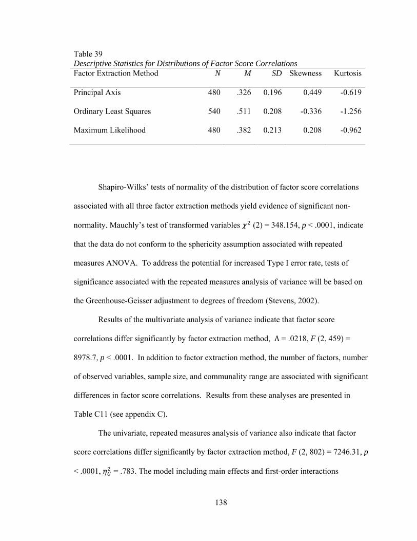
138
Table 39 Descriptive Statistics for Distributions of Factor Score Correlations Factor Extraction Method N M SD Skewness Kurtosis
Principal Axis 480 .326 0.196 0.449 -0.619
Ordinary Least Squares 540 .511 0.208 -0.336 -1.256
Maximum Likelihood 480 .382 0.213 0.208 -0.962
Shapiro-Wilks’ tests of normality of the distribution of factor score correlations
associated with all three factor extraction methods yield evidence of significant non-
normality. Mauchly’s test of transformed variables (2) = 348.154, p < .0001, indicate
that the data do not conform to the sphericity assumption associated with repeated
measures ANOVA. To address the potential for increased Type I error rate, tests of
significance associated with the repeated measures analysis of variance will be based on
the Greenhouse-Geisser adjustment to degrees of freedom (Stevens, 2002).
Results of the multivariate analysis of variance indicate that factor score
correlations differ significantly by factor extraction method, Λ = .0218, F (2, 459) =
8978.7, p < .0001. In addition to factor extraction method, the number of factors, number
of observed variables, sample size, and communality range are associated with significant
differences in factor score correlations. Results from these analyses are presented in
Table C11 (see appendix C).
The univariate, repeated measures analysis of variance also indicate that factor
score correlations differ significantly by factor extraction method, F (2, 802) = 7246.31, p
< .0001, = .783. The model including main effects and first-order interactions
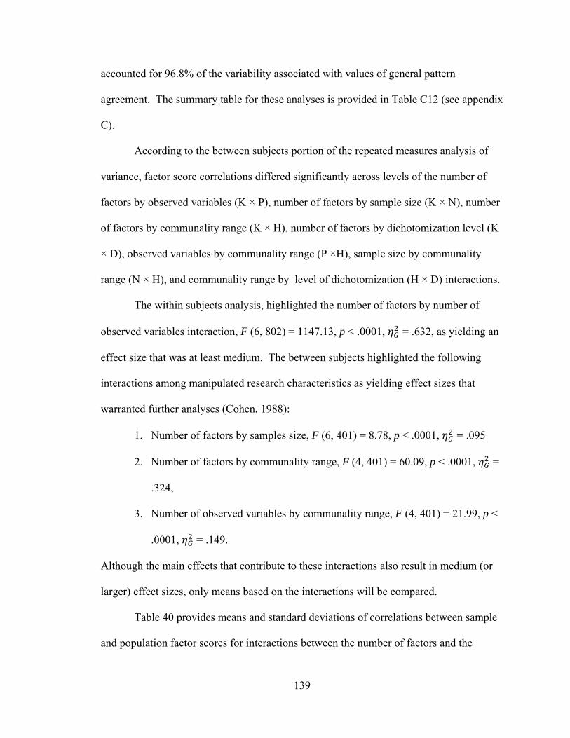
139
accounted for 96.8% of the variability associated with values of general pattern
agreement. The summary table for these analyses is provided in Table C12 (see appendix
C).
According to the between subjects portion of the repeated measures analysis of
variance, factor score correlations differed significantly across levels of the number of
factors by observed variables (K × P), number of factors by sample size (K × N), number
of factors by communality range (K × H), number of factors by dichotomization level (K
× D), observed variables by communality range (P ×H), sample size by communality
range (N × H), and communality range by level of dichotomization (H × D) interactions.
The within subjects analysis, highlighted the number of factors by number of
observed variables interaction, F (6, 802) = 1147.13, p < .0001, = .632, as yielding an
effect size that was at least medium. The between subjects highlighted the following
interactions among manipulated research characteristics as yielding effect sizes that
warranted further analyses (Cohen, 1988):
1. Number of factors by samples size, F (6, 401) = 8.78, p < .0001, = .095
2. Number of factors by communality range, F (4, 401) = 60.09, p < .0001, =
.324,
3. Number of observed variables by communality range, F (4, 401) = 21.99, p <
.0001, = .149.
Although the main effects that contribute to these interactions also result in medium (or
larger) effect sizes, only means based on the interactions will be compared.
Table 40 provides means and standard deviations of correlations between sample
and population factor scores for interactions between the number of factors and the

140
number of observed variables. The only interaction level in which ordinary least squares
does not yield the highest levels of correlation is the level that includes four factors and
20 observed variables; in this case, maximum likelihood yields a higher correlation. The
strongest correlation is associated with ordinary least squares in the two-factor by 20
observed variable condition.
Table 40 Means and Standard Deviations of Factor Score Correlations for Factor Extraction Methods and the Number of Factors by Observed Variables Interaction (K x P)
Principal Axis
Ordinary
Least Squares
Maximum
Likelihood
Interaction (K x P) M SD M SD M SD
2 × 20 .661 0.080 .726 0.070 .725 0.066
2 × 40 .091 0.083 .706 0.053 .112 0.096
2 × 60 - - .705 0.059 - -
4 × 20 .435 0.106 .473 0.094 .505 0.088
4 × 40 .417 0.075 .578 0.072 .516 0.047
4 × 60 .416 0.124 .641 0.073 .515 0.108
8 × 20 .137 0.040 .178 0.042 .163 0.027
8 × 40 .216 0.064 .265 0.050 .239 0.060
8 × 60 .234 0.074 .321 0.058 .278 0.064
N = 480
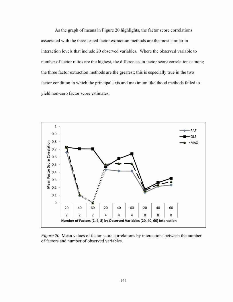
141
As the graph of means in Figure 20 highlights, the factor score correlations
associated with the three tested factor extraction methods are the most similar in
interaction levels that include 20 observed variables. Where the observed variable to
number of factor ratios are the highest, the differences in factor score correlations among
the three factor extraction methods are the greatest; this is especially true in the two
factor condition in which the principal axis and maximum likelihood methods failed to
yield non-zero factor score estimates.
Figure 20. Mean values of factor score correlations by interactions between the number of factors and number of observed variables.
0
0.1
0.2
0.3
0.4
0.5
0.6
0.7
0.8
0.9
1
20 40 60 20 40 60 20 40 60
2 2 2 4 4 4 8 8 8
Mean
Factor Score Correlation
Number of Factors (2, 4, 8) by Observed Variables (20, 40, 60) Interaction
PAF
OLS
MAX

142
The negative relationship between factor score correlation and the number of
factors is the only relationship that is common to all three factor extraction methods at all
levels of the interaction. Within the eight factor conditions of the interaction, both the
graphed means and the box plots (see Figure D22 in appendix D) indicate that the mean
and median factor score correlations increase as the number of observed variables
increase.
Table 41 provides means and standard deviations for factor score correlations by
factor extraction method and levels of the number of factors by sample size interaction.
In all levels of this interaction effect, ordinary least squares yielded the highest levels of
correlation between the sample and population in terms of factor scores. The strongest
correlation between sample and population is associated with the two factor condition in
which sample size equals 1000.
Across all factor extraction methods and levels of the interaction, box and whisker
plots (see Figure D23 in appendix D) indicate the median factor score correlations are
positively related to sample size within each number of factors condition and, for the
ordinary least square condition, negatively related to the number of factors.
Except for the conditions that include two factors, this negative relationship is also
apparent in the maximum likelihood and the principal axis factor extraction methods. In
maximum likelihood and principal axis factor extraction methods, the ranges and
interquartile ranges shrink substantially between the two and four factor conditions of the
interaction; this effect may be related to the diminished sample sizes in the two factor
conditions associated with both maximum likelihood and principal axis factor extraction
methods.

143
Figure 21 demonstrates that the differences among the three factor extraction
methods in terms of factor correlations diminish as the number of factors increases. The
largest difference among the factor analytic strategies is associated with the K = 2, N =
100 condition.
Table 41 Means and Standard Deviations of Factor Score Correlations for Factor Extraction Method and Number of Factors by Sample Size Interaction (K x N)
Principal Axis
Ordinary
Least Squares
Maximum
Likelihood
Interaction (K x N) M SD M SD M SD
2 × 100 .347 0.276 .680 0.053 .420 0.309
2 × 200 .371 0.296 .711 0.056 .417 0.322
2 × 300 .382 0.305 .725 0.058 .417 0.326
2 × 1000 .404 0.323 .751 0.063 .419 0.332
4 × 100 .337 0.094 .483 0.089 .461 0.087
4 × 200 .405 0.082 .548 0.091 .509 0.076
4 × 300 .440 0.080 .581 0.090 .525 0.073
4 × 1000 .510 0.076 .644 0.087 .553 0.077
8 × 100 .149 0.049 .218 0.061 .175 0.048
8 × 200 .184 0.063 .246 0.069 .220 0.061
8 × 300 .203 0.069 .261 0.074 .238 0.066
8 × 1000 .247 0.078 .296 0.086 .274 0.071
N = 480
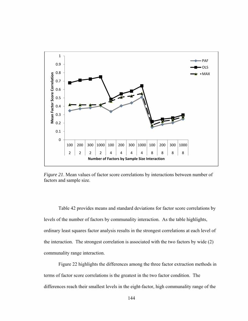
144
Figure 21. Mean values of factor score correlations by interactions between number of factors and sample size.
Table 42 provides means and standard deviations for factor score correlations by
levels of the number of factors by communality interaction. As the table highlights,
ordinary least squares factor analysis results in the strongest correlations at each level of
the interaction. The strongest correlation is associated with the two factors by wide (2)
communality range interaction.
Figure 22 highlights the differences among the three factor extraction methods in
terms of factor score correlations is the greatest in the two factor condition. The
differences reach their smallest levels in the eight-factor, high communality range of the
0
0.1
0.2
0.3
0.4
0.5
0.6
0.7
0.8
0.9
1
100 200 300 1000 100 200 300 1000 100 200 300 1000
2 2 2 2 4 4 4 4 8 8 8 8
Mean
Factor Score Correlation
Number of Factors by Sample Size Interaction
PAF
OLS
MAX
145
interaction. The graphed means and box and whisker plots (see Figure D24 in appendix
D) indicate that, mean and median factor score correlations for the ordinary least squares
factor extraction method are positively related to communality range and negatively
related to the number of factors; with the exception of the conditions containing two
factors, this relationship is also apparent in distributions of correlations yielded by
maximum likelihood and principal axis factor extraction methods.
Table 42 Means and Standard Deviations of Factor Score Correlations for Factor Extraction Method and Number of Factors by Communality Range Interaction (K x H)
Principal Axis
Ordinary
Least Squares
Maximum
Likelihood
Interaction (K x H) M SD M SD M SD
2 × Low .367 0.300 .720 0.062 .437 0.336
2 × Wide .443 0.443 .746 0.059 .474 0.263
2 × High .318 0.318 .683 0.051 .344 0.343
4 × Low .358 0.358 .539 0.140 .491 0.070
4 × Wide .419 0.419 .564 0.088 .478 0.059
4 × High .492 0.492 .589 0.074 .569 0.092
8 × Low .146 0.146 .212 0.080 .194 0.064
8 × Wide .192 0.192 .253 0.056 .220 0.052
8 × High .250 0.249 .299 0.071 .267 0.076
N = 480

146
Figure 22. Mean values of factor score correlations by interactions between number of factors and communality.
Table 43 provides means and standard deviations of factor score correlations for
factor extraction method by the number of variables and communality range interaction
effect. Except for the low 20 observed variable by low communality range condition,
ordinary least squares yields the highest levels of correlation between factor scores
associated with the population and the sample. The strongest correlation is associated
with the ordinary least squares factor extraction method at the P = 40, H = 2 (wide)
interaction level.
0
0.1
0.2
0.3
0.4
0.5
0.6
0.7
0.8
0.9
1
Low Wide High Low Wide High Low Wide High
2 2 2 4 4 4 8 8 8
Mean
Factor Score Correlation
Number of Factors by Communality Level Interaction
PAF
OLS
MAX
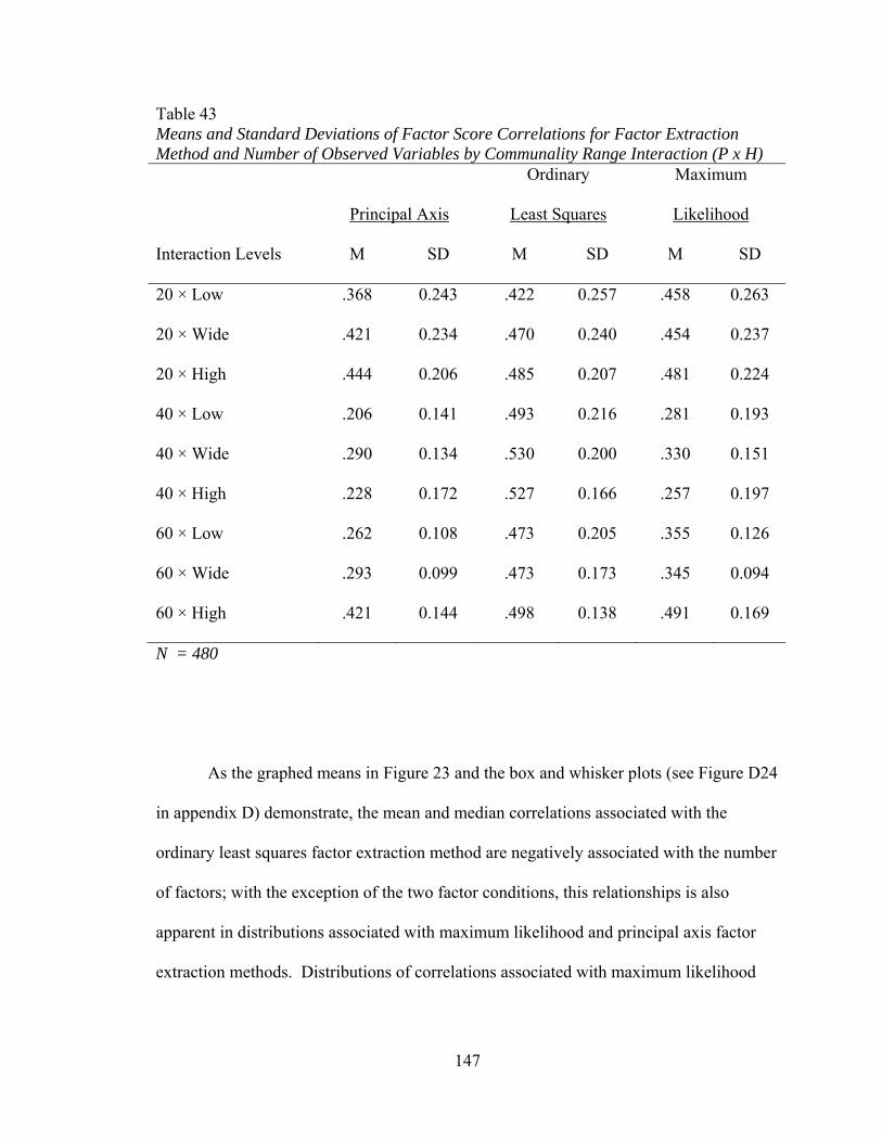
147
Table 43 Means and Standard Deviations of Factor Score Correlations for Factor Extraction Method and Number of Observed Variables by Communality Range Interaction (P x H)
Principal Axis
Ordinary
Least Squares
Maximum
Likelihood
Interaction Levels M SD M SD M SD
20 × Low .368 0.243 .422 0.257 .458 0.263
20 × Wide .421 0.234 .470 0.240 .454 0.237
20 × High .444 0.206 .485 0.207 .481 0.224
40 × Low .206 0.141 .493 0.216 .281 0.193
40 × Wide .290 0.134 .530 0.200 .330 0.151
40 × High .228 0.172 .527 0.166 .257 0.197
60 × Low .262 0.108 .473 0.205 .355 0.126
60 × Wide .293 0.099 .473 0.173 .345 0.094
60 × High .421 0.144 .498 0.138 .491 0.169
N = 480
As the graphed means in Figure 23 and the box and whisker plots (see Figure D24
in appendix D) demonstrate, the mean and median correlations associated with the
ordinary least squares factor extraction method are negatively associated with the number
of factors; with the exception of the two factor conditions, this relationships is also
apparent in distributions associated with maximum likelihood and principal axis factor
extraction methods. Distributions of correlations associated with maximum likelihood
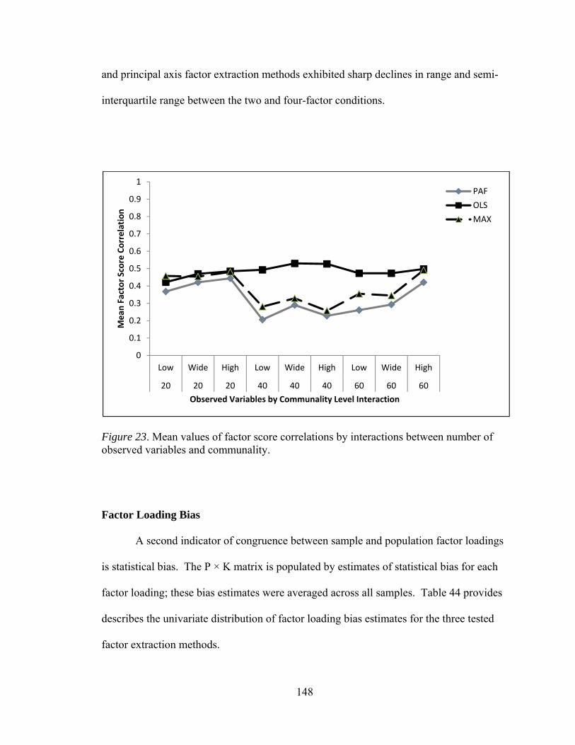
148
and principal axis factor extraction methods exhibited sharp declines in range and semi-
interquartile range between the two and four-factor conditions.
Figure 23. Mean values of factor score correlations by interactions between number of observed variables and communality.
Factor Loading Bias
A second indicator of congruence between sample and population factor loadings
is statistical bias. The P × K matrix is populated by estimates of statistical bias for each
factor loading; these bias estimates were averaged across all samples. Table 44 provides
describes the univariate distribution of factor loading bias estimates for the three tested
factor extraction methods.
0
0.1
0.2
0.3
0.4
0.5
0.6
0.7
0.8
0.9
1
Low Wide High Low Wide High Low Wide High
20 20 20 40 40 40 60 60 60
Mean
Factor Score Correlation
Observed Variables by Communality Level Interaction
PAF
OLS
MAX
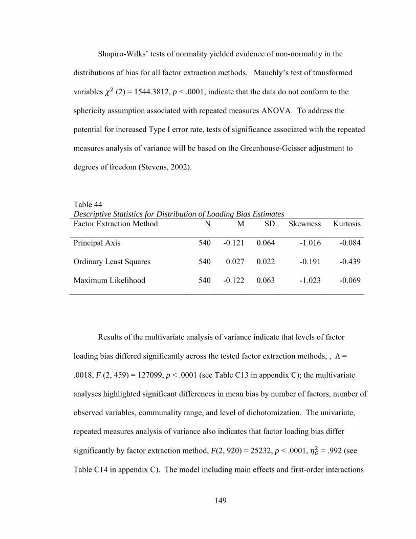
149
Shapiro-Wilks’ tests of normality yielded evidence of non-normality in the
distributions of bias for all factor extraction methods. Mauchly’s test of transformed
variables (2) = 1544.3812, p < .0001, indicate that the data do not conform to the
sphericity assumption associated with repeated measures ANOVA. To address the
potential for increased Type I error rate, tests of significance associated with the repeated
measures analysis of variance will be based on the Greenhouse-Geisser adjustment to
degrees of freedom (Stevens, 2002).
Table 44 Descriptive Statistics for Distribution of Loading Bias Estimates Factor Extraction Method N M SD Skewness Kurtosis
Principal Axis 540 -0.121 0.064 -1.016 -0.084
Ordinary Least Squares 540 0.027 0.022 -0.191 -0.439
Maximum Likelihood 540 -0.122 0.063 -1.023 -0.069
Results of the multivariate analysis of variance indicate that levels of factor
loading bias differed significantly across the tested factor extraction methods, , Λ =
.0018, F (2, 459) = 127099, p < .0001 (see Table C13 in appendix C); the multivariate
analyses highlighted significant differences in mean bias by number of factors, number of
observed variables, communality range, and level of dichotomization. The univariate,
repeated measures analysis of variance also indicates that factor loading bias differ
significantly by factor extraction method, F(2, 920) = 25232, p < .0001, = .992 (see
Table C14 in appendix C). The model including main effects and first-order interactions

150
accounted for 99.49% of the variability associated with statistical bias in factor pattern
matrices.
In addition to the method main effects, the multivariate and repeated measures
analyses of variance identified significant differences in bias associated with six of the
ten first-order interactions. However, only four of these interactions yielded effect sizes
that were medium or greater. These interactions included
1. Number of factors by observed variables, F(4, 460) = 244.87, p < .0001, =
.621
2. Number of factors by sample size, F(6, 460) = 15.62, p < .0001, = .136
3. Number of factors by level of communality, F(4, 460) = 454.50, p < .0001, =
.753
4. Number of factors by level of dichotomization, F(8, 460) = 4.91, p < .0001, =
.062
Comparisons among means were conducted for these interactions only.
Table 45 presents mean factor loading biases by for each factor extraction method
by each level of the interaction between number of factors and number of observed
variables. For each level of the interaction, the comparisons indicate that mean bias
values for ordinary least squares are closer to zero than they are for either the maximum
likelihood or the principal axis methods. Biases for principal axis and maximum
likelihood are negative. As both Table 42 and Figure 24 highlight, bias levels decrease as
the number of factors increase. This relationship is more strongly expressed in the
distributions associated with principal axis and maximum likelihood factor extraction
methods than it is in distributions associated with ordinary least squares.
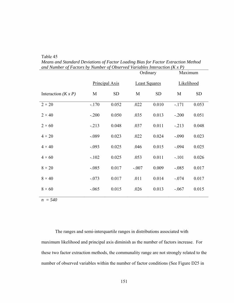
151
Table 45 Means and Standard Deviations of Factor Loading Bias for Factor Extraction Method and Number of Factors by Number of Observed Variables Interaction (K x P)
Principal Axis
Ordinary
Least Squares
Maximum
Likelihood
Interaction (K x P) M SD M SD M SD
2 × 20 -.170 0.052 .022 0.010 -.171 0.053
2 × 40 -.200 0.050 .035 0.013 -.200 0.051
2 × 60 -.213 0.048 .037 0.011 -.213 0.048
4 × 20 -.089 0.023 .022 0.024 -.090 0.023
4 × 40 -.093 0.025 .046 0.015 -.094 0.025
4 × 60 -.102 0.025 .053 0.011 -.101 0.026
8 × 20 -.085 0.017 -.007 0.009 -.085 0.017
8 × 40 -.073 0.017 .011 0.014 -.074 0.017
8 × 60 -.065 0.015 .026 0.013 -.067 0.015
n = 540
The ranges and semi-interquartile ranges in distributions associated with
maximum likelihood and principal axis diminish as the number of factors increase. For
these two factor extraction methods, the communality range are not strongly related to the
number of observed variables within the number of factor conditions (See Figure D25 in

152
appendix D). In distributions of bias associated with the ordinary least squares factor
extraction method, the mean and median levels of bias are positively related to the ratio
of observed variables to factors across all levels of the interaction.
Figure 24. Mean value of factor loading bias by interactions between number of factors by number of observed variables.
Table 46 provides means and standard deviations for mean bias levels across
factor extraction methods and levels of the number of factors by sample size interaction.
As was the case with the previous set of comparisons, the levels of bias decrease as the
number of factors increase. At the eight-factor by N = 100 condition, ordinary least
‐0.5
‐0.4
‐0.3
‐0.2
‐0.1
0
0.1
0.2
0.3
0.4
0.5
20 40 60 20 40 60 20 40 60
2 2 2 4 4 4 8 8 8
Mean
Factor Load
ings Bias
Number of Factors by Observed Variables Interaction
PAF
OLS
MAX

153
squares yields a mean bias of -.002; this is the smallest average amount of bias across all
factor methods and all interactions between number of factors and sample size.
Table 46 Means and Standard Deviations of Factor Loading Bias by Factor Extraction Method and Number of Factors by Sample Size Interaction (K x N)
Principal Axis
Ordinary
Least Squares
Maximum
Likelihood
Interaction (K x N) M SD M SD M SD
2 × 100 -.198 0.054 .030 0.011 -.200 0.064
2 × 200 -.195 0.054 .032 0.013 -.200 0.054
2 × 300 -.194 0.054 .032 0.013 -.194 0.054
2 × 1000 -.192 0.054 .033 0.016 -.193 0.054
4 × 100 -.103 0.022 .029 0.024 -.103 0.022
4 × 200 -.095 0.024 .040 0.021 -.095 0.024
4 × 300 -.093 0.025 .043 0.020 -.092 0.025
4 × 1000 -.088 0.028 .048 0.018 -.089 0.027
8 × 100 -.085 0.016 -.002 0.015 -.085 0.015
8 × 200 -.076 0.016 .008 0.017 -.077 0.016
8 × 300 -.072 0.017 .013 0.017 -.073 0.017
8 × 1000 -.065 0.017 .020 0.017 -.066 0.017
N = 540
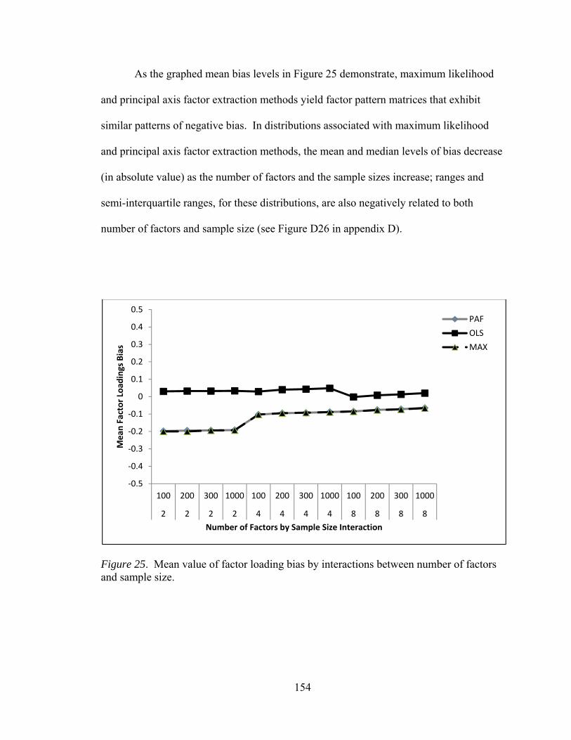
154
As the graphed mean bias levels in Figure 25 demonstrate, maximum likelihood
and principal axis factor extraction methods yield factor pattern matrices that exhibit
similar patterns of negative bias. In distributions associated with maximum likelihood
and principal axis factor extraction methods, the mean and median levels of bias decrease
(in absolute value) as the number of factors and the sample sizes increase; ranges and
semi-interquartile ranges, for these distributions, are also negatively related to both
number of factors and sample size (see Figure D26 in appendix D).
Figure 25. Mean value of factor loading bias by interactions between number of factors and sample size.
‐0.5
‐0.4
‐0.3
‐0.2
‐0.1
0
0.1
0.2
0.3
0.4
0.5
100 200 300 1000 100 200 300 1000 100 200 300 1000
2 2 2 2 4 4 4 4 8 8 8 8
Mean
Factor Load
ings Bias
Number of Factors by Sample Size Interaction
PAF
OLS
MAX

155
Table 47 provides means and standard deviations of loading bias estimates for the
three factor extraction methods by all levels of the number of factors by communality
range interaction. For maximum likelihood and principal axis factor extraction methods,
all mean levels of factor loading bias are negative. Ordinary least squares yields factor
loading bias estimates that are closer to zero than the other two factor extraction methods.
The smallest mean level of factor loading bias is associated with the eight-factor by low
communality condition (<.001 and > 0).
Table 47 Means and Standard Deviations of Factor Loading Bias for Factor Extraction Method and Number of Factors by Communality Range Interaction (K x H)
Principal Axis
Ordinary
Least Squares
Maximum
Likelihood
Interaction (K x H) M SD M SD M SD
2 × Low -.132 0.021 .027 0.010 -.132 0.022
2 × Wide -.200 0.018 .030 0.010 -.200 0.018
2 × High -.253 0.019 .037 0.017 -.253 0.019
4 × Low -.065 0.009 .025 0.020 -.066 0.009
4 × Wide -.097 0.009 .039 0.019 -.098 0.009
4 × High -.121 0.011 .056 0.014 -.121 0.011
8 × Low -.058 0.011 <.001 0.017 -.058 0.011
8 × Wide -.073 0.010 .011 0.015 -.075 0.009
8 × High -.092 0.013 .019 0.018 -.092 0.013
N = 540

156
In the distributions of bias associated with maximum likelihood and principal axis
factor extraction methods, the graphed means in Figure 26 and box and whisker plots (see
Figure D27 in appendix D) indicate that the absolute values of bias are positively related
to communality and negatively related to the number of factors imbedded in the
population. This pattern is not expressed in the distribution of bias values for ordinary
least squares.
Figure 26. Mean value of factor loading bias by interactions between number of factors and communality.
‐0.5
‐0.4
‐0.3
‐0.2
‐0.1
0
0.1
0.2
0.3
0.4
0.5
Low Wide High Low Wide High Low Wide High
2 2 2 4 4 4 8 8 8
Mean
Facror Load
ings Bias
Number of Factors by Communlaity Level Interaction
PAF
OLS
MAX

157
In the distributions of bias associated with maximum likelihood and principal axis
factor extraction methods, the graphed means in Figure 26 and box and whisker plots (see
Figure D27 in appendix D) indicate that the absolute values of bias are positively related
to communality and negatively related to the number of factors imbedded in the
population. This pattern is not expressed in the distribution of bias values for ordinary
least squares.
Table 48 includes means and standard deviations of factor loading bias values for
each level of the interaction between number of factors and level of dichotomization
interaction. The mean biase values for principal axis and maximum likelihood factor
extraction methods are negative for each level of the interaction. Across all levels of the
interaction, ordinary least squares resulted in the smallest mean amount of factor loading
bias.
The graphed means in Figure 27 and box and whisker plots (see Figure D28 in
appendix D) indicate that the absolute values of means and median levels of statistical
bias in the factor loading matrices diminish as the number of factors increase. For
maximum likelihood and principal axis factor extraction methods, the ranges and semi-
interquartile ranges also diminish as the number of factors increase. These patterns in
measures of central tendency and dispersion are not apparent in the distributions of
loading bias associated with the ordinary least squares factor extraction method.
Across all significant interactions, ordinary least squares factor extraction method
yielded factor loading matrices that exhibited smaller mean values of statistical bias than
matrices derived from the principal axis and the maximum likelihood methods.

158
Table 48 Means and Standard Deviations of Factor Loading Bias for Factor Extraction Method and Number of Factors by Level of Dichotomization Interaction (K x D)
Principal Axis
Ordinary
Least Squares
Maximum
Likelihood
Interaction (K x D) M SD M SD M SD
2 × .05 -.194 0.059 .033 0.012 -.194 0.059
2 × .25 -.194 0.055 .031 0.014 -.194 0.055
2 × .50 -.190 0.050 .038 0.014 -.190 0.050
2 × .75 -.197 0.053 .024 0.013 -.197 0.052
2 × .95 -.200 0.053 .031 0.011 -.200 0.053
4 × .05 -.096 0.025 .040 0.022 -.096 0.025
4 × .25 -.092 0.025 .043 0.022 -.093 0.025
4 × .50 -.093 0.025 .041 0.023 -.094 0.025
4 × .75 -.094 0.025 .040 0.020 -.095 0.025
4 × .95 -.097 0.026 .038 0.023 -.098 0.026
8 × .05 -.073 0.017 .011 0.017 -.074 0.017
8 × .25 -.073 0.018 .012 0.019 -.073 0.018
8 × .50 -.074 0.018 .010 0.019 -.075 0.018
8 × .75 -.075 0.018 .009 0.017 -.075 0.018
8 × .95 -.078 0.019 .007 0.020 -.079 0.018
N = 540
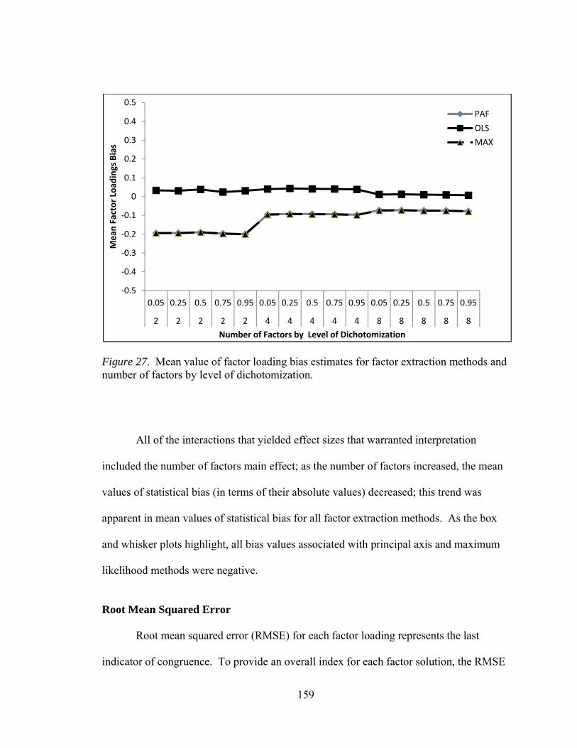
159
Figure 27. Mean value of factor loading bias estimates for factor extraction methods and number of factors by level of dichotomization.
All of the interactions that yielded effect sizes that warranted interpretation
included the number of factors main effect; as the number of factors increased, the mean
values of statistical bias (in terms of their absolute values) decreased; this trend was
apparent in mean values of statistical bias for all factor extraction methods. As the box
and whisker plots highlight, all bias values associated with principal axis and maximum
likelihood methods were negative.
Root Mean Squared Error Root mean squared error (RMSE) for each factor loading represents the last
indicator of congruence. To provide an overall index for each factor solution, the RMSE
‐0.5
‐0.4
‐0.3
‐0.2
‐0.1
0
0.1
0.2
0.3
0.4
0.5
0.05 0.25 0.5 0.75 0.95 0.05 0.25 0.5 0.75 0.95 0.05 0.25 0.5 0.75 0.95
2 2 2 2 2 4 4 4 4 4 8 8 8 8 8
Mean
Factor Load
ings Bias
Number of Factors by Level of Dichotomization
PAF
OLS
MAX
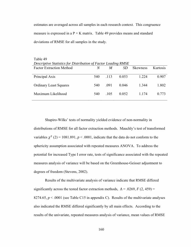
160
estimates are averaged across all samples in each research context. This congruence
measure is expressed in a P × K matrix. Table 49 provides means and standard
deviations of RMSE for all samples in the study.
Table 49 Descriptive Statistics for Distribution of Factor Loading RMSE Factor Extraction Method N M SD Skewness Kurtosis
Principal Axis 540 .113 0.053 1.224 0.907
Ordinary Least Squares 540 .091 0.046 1.344 1.802
Maximum Likelihood 540 .105 0.052 1.174 0.773
Shapiro-Wilks’ tests of normality yielded evidence of non-normality in
distributions of RMSE for all factor extraction methods. Mauchly’s test of transformed
variables (2) = 1081.891, p < .0001, indicate that the data do not conform to the
sphericity assumption associated with repeated measures ANOVA. To address the
potential for increased Type I error rate, tests of significance associated with the repeated
measures analysis of variance will be based on the Greenhouse-Geisser adjustment to
degrees of freedom (Stevens, 2002).
Results of the multivariate analysis of variance indicate that RMSE differed
significantly across the tested factor extraction methods, Λ = .0269, F (2, 459) =
8274.65, p < .0001 (see Table C15 in appendix C). Results of the multivariate analyses
also indicated the RMSE differed significantly by all main effects. According to the
results of the univariate, repeated measures analysis of variance, mean values of RMSE
161
differed significantly by factor extraction method, F(2, 920) = 1559.4, p < .0001, =
.458 (see Table C16 in appendix C). The model including main effects and first-order
interactions accounted for 96.26% of the variability associated with statistical bias in
factor pattern matrices.
In addition to the method effect, the multivariate and repeated measures analyses
of variance identified significant differences in RMSE associated with seven of the ten
first-order interactions. However, according to the within subjects and the between
subjects portions of the repeated measures analysis of variance, only four of these
interactions yield effect sizes that were medium or greater. These interaction include
1. Number of factors by number of observed variables, F(4, 460) = 209.92, p <
.0001, = .578
2. Number of factors by level of communality, F(4, 460) = 548.08, p < .0001,
= .781
3. Number of factors by level of dichotomization, F(8, 460) = 9.99, p < .0001,
= .115
4. Level of communality by level of dichotomization, F(8, 460) = 6.73, p <
.0001, = .081
In addition to these interactions, the sample size main effect yielded an effect size of at
least medium strength, F(3, 460) = 172.94, p < .0001, = .458. Because sample size is
not included in interactions that met the effect size criteria for further analyses, it will
also be included in the comparisons among means.
Table 47 presents means and standard deviations of RMSE for each factor
extraction method by each level of sample size.

162
Table 50 Means and Standard Deviations of Factor Loading RMSE for Factor Extraction Method by Sample Size
Principal Axis
Ordinary
Least Squares
Maximum
Likelihood
Effect Levels M SD M SD M SD
100 .124 0.052 .114 0.046 .112 0.049
200 .115 0.053 .094 0.044 .105 0.052
300 .111 0.053 .085 0.043 .103 0.052
1000 .104 0.053 .071 0.041 .099 0.054
N = 540
As the table highlights, RMSE is negatively related to sample size. Results of the
comparison indicate that principal axis factor analysis yields the highest values of RMSE.
Moreover, except for the N = 100 condition, ordinary least squares yields the lowest
levels of RMSE.
The relationship among sample size, factor extraction method, and mean RMSE is
demonstrated graphically in Figure 28. As this graph highlights, the negative relationship
between sample size and RMSE is slightly more apparent in the trend associated with the
ordinary least squares factor extraction method.

163
Figure 28. Mean value of RMSE by sample size main effect.
Table 51 presents means and standard deviation of mean RMSE values for each
factor extraction method by levels of the number of factors and observed variables
interaction. The mean RMSE values do not have a simple relationship with either effect
included in the interaction. However, the ordinary least squares factor extraction method
yields slightly smaller values of RMSE than either principal axis or maximum likelihood
factor extraction methods.
As the trend lines in Figure 29 highlight, the differences among factor extraction
methods in mean values of RMSE do not appear to vary substantially as either the
number of factors or the number of observed variables increases.
0
0.05
0.1
0.15
0.2
0.25
100 200 300 1000
Mean
Factor Load
ing RMSE
Sample Size
PAF
OLS
MAX

164
Table 51 Means and Standard Deviations of Factor Loading RMSE for Factor Extraction Method and Number of Factors by Observed Variables (K x P)
Principal Axis
Ordinary
Least Squares
Maximum
Likelihood
Interaction (K x P) M SD M SD M SD
2 × 20 .142 0.058 .124 0.056 .127 0.059
2 × 40 .164 0.061 .132 0.054 .150 0.061
2 × 60 .174 0.063 .133 0.052 .164 0.063
4 × 20 .109 0.023 .095 0.026 .098 0.024
4 × 40 .092 0.027 .079 0.022 .083 0.028
4 × 60 .090 0.030 .070 0.023 .083 0.030
8 × 20 .110 0.012 .079 0.014 .104 0.014
8 × 40 .075 0.013 .059 0.016 .072 0.015
8 × 60 .064 0.013 .048 0.015 .061 0.014
N = 540
For all factor extraction methods, box and whisker plots of RMSE values
highlight a general decline in ranges and semi-interquartile ranges as the number of
factors increases (See Figure D29 in appendix D). Within the four and eight-factor
conditions, mean and median RMSE values decline as the ratio of observed variables to
factors increases.
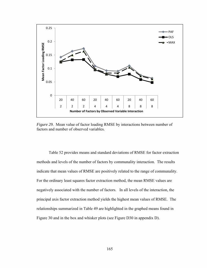
165
Figure 29. Mean value of factor loading RMSE by interactions between number of factors and number of observed variables.
Table 52 provides means and standard deviations of RMSE for factor extraction
methods and levels of the number of factors by communality interaction. The results
indicate that mean values of RMSE are positively related to the range of communality.
For the ordinary least squares factor extraction method, the mean RMSE values are
negatively associated with the number of factors. In all levels of the interaction, the
principal axis factor extraction method yields the highest mean values of RMSE. The
relationships summarized in Table 49 are highlighted in the graphed means found in
Figure 30 and in the box and whisker plots (see Figure D30 in appendix D).
0
0.05
0.1
0.15
0.2
0.25
20 40 60 20 40 60 20 40 60
2 2 2 4 4 4 8 8 8
Mean
Factor Load
ing RMSE
Number of Factors by Observed Variable Interaction
PAF
OLS
MAX

166
Table 52 Means and Standard Deviations of Factor Loading RMSE for Factor Extraction Method and Number of Factors by Communality Range Interaction (K x H)
Principal Axis
Ordinary
Least Squares
Maximum
Likelihood
Interaction (K x H) M SD M SD M SD
2 × Low .090 0.015 .084 0.022 .074 0.014
2 × Wide .155 0.022 .121 0.038 .147 0.020
2 × High .233 0.022 .184 0.041 .221 0.021
4 × Low .067 0.018 .061 0.023 .055 0.015
4 × Wide .098 0.013 .085 0.020 .091 0.011
4 × High .126 0.010 .098 0.019 .118 0.007
8 × Low .070 0.022 .058 0.021 .063 0.020
8 × Wide .082 0.020 .063 0.019 .080 0.019
8 × High .097 0.020 .064 0.019 .094 0.019
N = 540

167
Figure 30. Mean value of factor loading by interactions between number of factors and communality.
As Table 53 presents highlights, the ordinary least squares method yielded the
lowest mean RMSE’s for all levels of the number of factors by dichotomization
interaction. Moreover, for all factor extraction methods, RMSE is negatively related to
the number of factors simulated in the population. In addition to mean values of RMSE,
box and whisker plots indicate that ranges and semi-interquartile ranges, for all
distributions, decrease as the number of factors increases (see Figure D31 in appendix D).
Figure 31 demonstrates the relationships summarized in Table 50 graphically.
0
0.05
0.1
0.15
0.2
0.25
Low Wide High Low Wide High Low Wide High
2 2 2 4 4 4 8 8 8
Mean
Factor Load
ing RMSE
Number of Factors by Communality Level Interaction
PAF
OLS
MAX

168
Table 53 Means and Standard Deviations of Factor Loading RMSE for Factor Extraction Method and Number of Factors by Level of Dichotomization Interaction (K x D)
Principal Axis
Ordinary
Least Squares
Maximum
Likelihood
Interaction (K x D) M SD M SD M SD
2 × .05 .158 0.069 .124 0.058 .147 0.068
2 × .25 .156 0.057 .114 0.034 .145 0.061
2 × .50 .156 0.061 .125 0.047 .143 0.062
2 × .75 .160 0.060 .133 0.057 .145 0.060
2 × .95 .169 0.064 .153 0.063 .155 0.060
4 × .05 .099 0.029 .087 0.026 .091 0.030
4 × .25 .097 0.028 .082 0.027 .089 0.030
4 × .50 .096 0.028 .078 0.026 .088 0.029
4 × .75 .095 0.027 .080 0.026 .086 0.028
4 × .95 .097 0.027 .081 0.024 .087 0.027
8 × .05 .084 0.023 .064 0.019 .080 0.023
8 × .25 .083 0.024 .062 0.020 .079 0.023
8 × .50 .083 0.024 .062 0.022 .079 0.024
8 × .75 .082 0.023 .061 0.020 .078 0.023
8 × .95 .083 0.024 .061 0.020 .080 0.024
N = 540
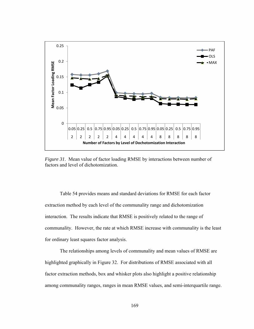
169
Figure 31. Mean value of factor loading RMSE by interactions between number of factors and level of dichotomization.
Table 54 provides means and standard deviations for RMSE for each factor
extraction method by each level of the communality range and dichotomization
interaction. The results indicate that RMSE is positively related to the range of
communality. However, the rate at which RMSE increase with communality is the least
for ordinary least squares factor analysis.
The relationships among levels of communality and mean values of RMSE are
highlighted graphically in Figure 32. For distributions of RMSE associated with all
factor extraction methods, box and whisker plots also highlight a positive relationship
among communality ranges, ranges in mean RMSE values, and semi-interquartile range.
0
0.05
0.1
0.15
0.2
0.25
0.05 0.25 0.5 0.75 0.95 0.05 0.25 0.5 0.75 0.95 0.05 0.25 0.5 0.75 0.95
2 2 2 2 2 4 4 4 4 4 8 8 8 8 8
Mean
Factor Load
ing RMSE
Number of Factors by Level of Dochotomization Interaction
PAF
OLS
MAX
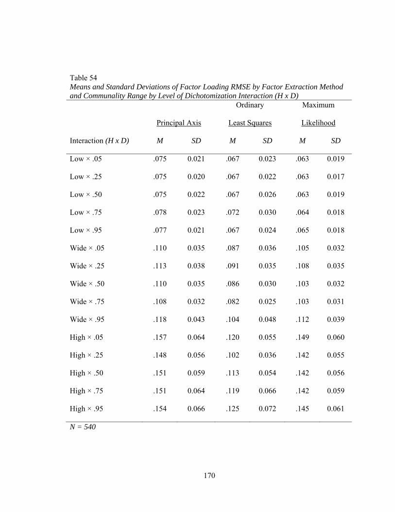
170
Table 54 Means and Standard Deviations of Factor Loading RMSE by Factor Extraction Method and Communality Range by Level of Dichotomization Interaction (H x D)
Principal Axis
Ordinary
Least Squares
Maximum
Likelihood
Interaction (H x D) M SD M SD M SD
Low × .05 .075 0.021 .067 0.023 .063 0.019
Low × .25 .075 0.020 .067 0.022 .063 0.017
Low × .50 .075 0.022 .067 0.026 .063 0.019
Low × .75 .078 0.023 .072 0.030 .064 0.018
Low × .95 .077 0.021 .067 0.024 .065 0.018
Wide × .05 .110 0.035 .087 0.036 .105 0.032
Wide × .25 .113 0.038 .091 0.035 .108 0.035
Wide × .50 .110 0.035 .086 0.030 .103 0.032
Wide × .75 .108 0.032 .082 0.025 .103 0.031
Wide × .95 .118 0.043 .104 0.048 .112 0.039
High × .05 .157 0.064 .120 0.055 .149 0.060
High × .25 .148 0.056 .102 0.036 .142 0.055
High × .50 .151 0.059 .113 0.054 .142 0.056
High × .75 .151 0.064 .119 0.066 .142 0.059
High × .95 .154 0.066 .125 0.072 .145 0.061
N = 540

171
Figure 32. Mean value of factor loading RMSE by interactions between communality and level of dichotomization.
Summary of Results
Factor extraction method accounted for statistically significant differences in all
measures of agreement between sample and population factor loading matrices. As
indicated by the generalized eta-squared values, factor extraction method accounted for
more than 90% of the variability in factor loading sensitivity ( = .998), general factor
loading pattern agreement ( = .991), and per element agreement ( = .934). Although
values of total factor pattern agreement differed significantly by factor extraction method,
the method effect accounted for less than 20% of the variance in this measure ( =
.198).
0
0.05
0.1
0.15
0.2
0.25
0.05 0.25 0.5 0.75 0.95 0.05 0.25 0.5 0.75 0.95 0.05 0.25 0.5 0.75 0.95
Low Low Low Low Low WideWideWideWideWide High High High High High
Mean
Factor Load
ing RMSE
Communality Level by Level of Dochotomization Interaction
PAF
OLS
MAX

172
The interaction between factor extraction method and the ratio of categorical
(dichotomous) variables to the total number of observed variables accounted for
statistically significant differences in only three measures of agreement between the
sample and the population. In the cases where statistical differences were observed, the
effect sizes were small (Cohen, 1988); these measures included factor loading sensitivity
( = .049), per element agreement ( = .003), and total pattern agreement ( = .025).
However, as part of a between subjects, first-order interaction with the number of factors
imbedded in the population, the level of dichotomization accounted for more than 57%
( = .574) of the variance in factor loading sensitivity. The comparison of means by
factor extraction method indicated that, for every level of this interaction, ordinary least
squares yielded higher mean values of factor loading sensitivity.
Interactions between the number of observed variables and factor extraction
method accounted for statistically and practically significant differences in all measures
of agreement between sample and population factor loading matrices. Within subjects
analyses indicated that the ratio of observed variables to number of factors imbedded in
the population yielded large effect sizes in loading sensitivity ( = .770), general pattern
agreement ( = .442), per element agreement ( = .474), and total pattern agreement
( = .436). These same analyses indicated that the number of observed variables
interacted with communality to yield at least a medium effect size in factor loading
sensitivity ( = .059). The between subject analysis indicated that the number of
variables interacted with communality to yield at least medium effect sizes in general
pattern agreement ( = .359) and per element agreement ( = .155). For all levels of
interactions among these main effects, ordinary least squares yielded significantly higher

173
mean values in all measures of agreement than either maximum likelihood or principal
axis factor extraction methods.
Sample size interacted with factor extraction method to yield significant
differences in mean values for all measures of agreement between sample and population
factor loading matrices. Between subjects analyses indicated that sample size interacted
with the number of factors imbedded in the population to yield a medium effect size in
per element agreement ( = .172); a within subjects analysis indicated that this first
order interaction yielded a medium effect size in total pattern agreement ( = .094). The
within subjects analysis also indicated that sample size and communality interacted to
yield medium effect sizes in general pattern agreement ( = .180) and per element
agreement ( = .077). For all levels of interactions among these main effects, ordinary
least squares yielded significantly higher mean values in all measures of agreement than
either maximum likelihood or principal axis factor extraction methods.
The levels of communality interacted with factor extraction method to yield
statistically significant differences in factor loading sensitivity, general pattern
agreement, and per element agreement. Between subjects analyses indicated that
interactions between level of communality and the number of factors imbedded in the
population yielded at least medium effects in factor loading sensitivity ( = .062),
general pattern agreement ( = .458), and per element agreement ( = .077). For all of
these measures, ordinary least squares yielded the highest mean values across all levels of
the interaction.
Factor extraction method accounted for statistically significant differences in all
measures of congruence. As indicated by the generalized eta-squared values, factor
174
extraction method accounted for more than 50% of the variability in three of the four
measures associated with sample and population congruence; these included mean phi
coefficient ( = .521), factor score correlations ( = .783), and factor loading bias (
= .992). Although values of factor loading RMSE differed significantly by factor
extraction method, the method effect accounted for less than 50% of the variance in this
measure ( = .458).
As a main effect, the ratio of categorical variables to the total number of observed
variables accounted for statistically significant differences in factor loading bias and
RMSE. Between subjects analyses indicated that interactions between level of
dichotomization and the number of factors imbedded in the population yielded at least
medium effect sizes in the mean values of the phi coefficient ( = .086), factor loading
bias ( = .458), and RMSE ( = .115). Between subjects analyses also indicated that
dichotomization interacted with communality to yield at least medium effect sizes in
mean phi coefficients ( = .076) and RMSE ( = .081). In general, maximum
likelihood yielded higher mean phi coefficients than either ordinary least squares or
maximum likelihood factor extraction methods. Across the majority of levels of the first-
order interactions, ordinary least yielded values of bias and RMSE that were closer to
zero than either maximum likelihood or principal axis factor extraction methods;
however, differences among the three factor extraction methods were small.
The number of observed variables main effect for statistically significant
differences in all of the congruence measures. Between subjects analyses indicated that
ratios of observed variables to factor yielded at least medium effect sizes in mean phi
coefficients ( = .405), factor score correlations ( = .804), factor loading bias ( =

175
.621), and RMSE ( = .578). These same analyses indicated that the interaction
between communality and the number of observed variables yielded an effect size that
was at least medium in factor score correlations ( = .149). Maximum likelihood
yielded higher mean phi coefficients across all ratios of observed variables to number of
factors than ordinary least squares or principal axis factor extraction methods. In the
majority of the levels of this interaction, ordinary least squares factor extraction method
resulted in stronger correlations between sample and population factor scores; in the four-
factor by 20 variable condition, maximum likelihood yielded a slightly higher correlation.
In the interaction between the number of observed variables and the level of
communality, ordinary least squares also yielded higher factor correlations in nearly all
levels of the interaction.
The sample size main effect yielded significant differences in mean values for
three measures of congruence among sample and population factor loading matrices;
these include mean phi coefficients, factor score correlations, RMSE. Between subjects
analyses indicated that the sample size interacted with the number of factors in the
population to yield at least medium effect sizes in mean phi coefficients ( = .115),
factor score correlations ( = .095), and factor loading bias ( = .136). Sample size
interacted with communality to yield an at least medium effect size in mean phi
coefficients ( = .067). Across all ratios of sample size to number of factors, maximum
likelihood yielded higher mean phi coefficients than ordinary least squares and principal
axis factor extraction methods. For nearly all levels of the sample size by number of
factors and sample size by communality interactions, ordinary least squares yielded
stronger correlations among sample and population factor score correlations. In nearly

176
all levels of sample size by number of factors interaction, ordinary least squares yielded
factor loading bias values that were closer to zero than either maximum likelihood or
principal axis factor extraction methods.
The communality main effect yielded statistically significant differences in all
congruence measures. Between subjects analyses indicated that interactions between
level of communality and the number of factors imbedded in the population yielded at
least medium effects in factor score correlations ( = .324), factor loading bias ( =
.753), and RMSE ( = .781). In all levels of the interaction, ordinary least squares
yielded stronger factor score correlations, factor score bias levels closer to zero, and
smaller values of RMSE.
Research Questions
How do varying ratios of categorical to continuous variables influence the
agreement between factor pattern matrices extracted through the examined factor
anlaysis strategies and factor pattern matrices simulated in the population? Level of
dichotomization resulted in significant differences in values of factor loading sensitivity,
per element factor pattern agreement, total pattern agreement, congruence, factor score
correlation, bias, and RMSE. As estimated by generalized eta squared, levels of
dichotomization accounted for medium effect size differences in values of factor loading
sensitivity and factor loading bias. However, in both cases, levels of dichotomization
were components of interactions that also resulted in effect sizes that were at least
medium. Therefore, the effects of dichotomization could only be interpreted as part of
first order interactions.

177
Dichotomization interacted with the number of factors to result in statistically and
practically significant differences factor loading sensitivity, congruence coefficients,
factor loading bias, and RMSE. In general, comparisons among means of these variables
based on the first order interactions indicated that the level of dichotomization did not
influence the impact that the number of factors had an on agreement and congruence
measures. However, within the two factor condition, mean values of the congruence
coefficient did exhibit a slight negative relationship to the level of dichotomization.
Levels of dichotomization and communality interacted to yield statistically and
practically significant differences in congruence coefficients and RMSE; comparisons
among means indicated that, in neither case, did the level of dichotomization exert
influence on the impact associated with communality.
How does the number of variables in a correlation matrix influence the agreement
between factor pattern matrices extracted through the examined factor analysis strategies
and factor pattern matrices simulated in the population? The number of observed
variables resulted in significant differences in values of factor loading sensitivity, general
pattern agreement, per element pattern agreement, total pattern agreement, congruence,
factor score correlation, bias, and RMSE. As estimated by generalized eta squared, the
observed variable main effect accounted for medium effect size differences in values of
factor loading sensitivity, general pattern agreement, per element pattern agreement, total
pattern agreement, congruence, factor score correlations, bias, and RMSE. However, in
all cases, the numbers of observed variables were components of interactions that also
resulted in effect sizes that were at least medium. Therefore, the impact of observed
variables could only be interpreted as part of first order interactions.

178
The number of observed variables interacted with the number of factors imbedded
in the population to yield differences in all measures of agreement and congruence that
reached effect sizes that warranted interpretation. For maximum likelihood and principal
axis factor extraction methods, values of factor loading sensitivity and general pattern
agreement were negatively related to the number of variables within each level of the
number of factors condition; for factor loading matrices associated with ordinary least
squares, these values were not influenced by the number of observed variables. The
direction of the relationship between the number of observed variables and values of per
element agreement changed with each level of the number of factors imbedded in the
population. Within each level of the number of common factors, values of congruence
were positively associated with the number of observed variables. In the eight factor
condition, this positive relationship with the number of observed variables is also present
in the correlations between factor scores in the sample and factor scores in the
population. However, in the two factor condition, the relationship between factor score
correlations and number of observed variables is negative for all factor extraction
methods. For both bias and RMSE, the relationship with number of observed variables
changed direction (positive versus negative) for each level of the number of factors
effect.
The number of observed variables interacted with the level of communality to
yield differences in all factor loading sensitivity, general pattern agreement, per element
agreement, and factor score correlation that were at least medium in effect sizes. While
values of factor loading sensitivity associated with the ordinary least squares method
were not influenced by the interaction between number of observed variables and

179
communality; the values of these measures were negatively related to the number of
variables for both maximum likelihood and principal axis factor extraction methods. For
the 40 and 60 observed variable conditions, factor score correlation appears to be
positively related to the number of observed variables within each level of communality;
however, this relationship is only apparent in maximum likelihood and principal axis
factor extraction methods.
How does sample size influence the agreement between factor pattern matrices
extracted through the examined factor analysis strategies and factor pattern matrices
simulated in the population? Sample size resulted in significant differences in values of
factor loading sensitivity, general pattern agreement, per element factor pattern
agreement, total pattern agreement, congruence, factor score correlation, and RMSE. As
estimated by generalized eta squared, the between subjects analysis indicated that sample
size accounted for medium effect size differences in values of general pattern agreement,
per element agreement, congruence coefficients, sample and population factor score
correlations, and RMSE. In the case of RMSE, the sample size main effect yielded an
effect size that was at least moderate without being a component of a substantial
interaction; for all three factor extraction methods, RMSE diminished as sample size
increased. In all other measures of agreement and congruence, sample size was a part of
interactions that met the effect size threshold for interpretation.
Sample size interacted with the number of factors imbedded in the population to yield
statistically and practically significant differences in per element agreement, total
agreement, congruence, correlations between sample and population factor scores, and
bias. In all measures of agreement between sample and population, the levels of

180
agreement were positively associated with sample size within each number of factors
condition. Because maximum likelihood and principal axis factor extraction methods
failed to yield non-zero factor scores in all conditions, a universally applicable trend is
difficult to identify; however, when the two factor conditions are ignored, correlations
among sample and population factor scores are positively related to sample size. Within
each number of factors condition, the amount of negative bias in solutions associated
with maximum likelihood and principal axis methods diminishes as the smaple size
increases; the amount of bias associated with the ordinary least squares method is not
influenced by sample size.
Differences in mean values for general pattern agreement, per element agreement,
and congruence of at least medium effect are associated with interactions between sample
size and communality. For all three methods, values of general pattern agreement and
congruence were positively related to sample size. Values of per element agreement
were positively associated with sample size in pattern matrices derived from the ordinary
least squares factor extraction method; this relationship was not apparent in maximum
likelihood or principal axis methods.
How does communality influence the agreement between factor pattern matrices
extracted through the examined factor analysis strategies and factor pattern matrices
simulated in the population? The level of communality (low, wide, and high) resulted in
significant differences in values of factor loading sensitivity, general pattern agreement,
per element pattern agreement, congruence, factor score correlation, bias, and RMSE. As
estimated by generalized eta squared, the communality main effect accounted for medium
effect size differences in values of factor loading sensitivity, general pattern agreement,

181
per element pattern agreement, congruence, factor score correlations, bias, and RMSE.
However, in all cases, the levels of communality were components of interactions that
also resulted in effect sizes that were at least medium. Therefore, the impact of
communality could only be interpreted as part of first order interactions.
The number of factors imbedded in the population interacts with communality to
yield differences in factor loading sensitivity, general pattern agreement, per element
agreement, factor score correlations, bias, and RMSE that are at least medium in effect
size. For maximum likelihood and principal axis factor extraction methods, values of
factor loading sensitivity are positively related to the level of communality within each
level of the interaction; values of factor loading sensitivity associated with ordinary least
squares are not influenced by communality within its interaction with the number of
factors. Within all levels of the interaction, values of general pattern agreement are
positively related to level of communality; this is true across all factor extraction
methods. In nearly all levels of the interaction, values of per element agreement are
negatively related to level of communality; however, for the ordinary least squares factor
extraction method, this relationship is slightly positive in the eight factor condition. In
the four and eight factor conditions, factor score correlations exhibit a generally positive
relationship with level of communality; however, this trend is not universal and not
apparent in the two factor conditions. For all three factor extraction methods, absolute
values of bias and RMSE are positively related to the level of communality within each
level of the number of factors condition.
The number of observed variables interacted with level of communality to yield
substantial differences in factor loading sensitivity, general pattern agreement and factor

182
score correlation. For maximum likelihood and principal axis factor extraction methods,
factor loading sensitivity is positively associated with the level of communality in all
levels of the interaction. However, this relationship is not apparent in loading sensitivity
values associated with ordinary least squares. In most levels of the interaction, values of
general pattern agreement are positively related to level of communality; however, for the
maximum likelihood factor extraction method, a slightly negative relationship between
general agreement and communality is apparent in the 60 observed variable condition.
The direction of the relationships among factor score correlations and communality levels
appears to vary by factor extraction method and level of the observed variables effect.
The sample size effect interacts with communality to yield differences in general
pattern agreement, per element agreement, and congruence. Within all levels of the
interaction and for all factor extraction methods, values of general pattern agreement are
positively related to level of communality. For the maximum likelihood and principal
axis factor extraction methods, values of per element agreement are negatively related to
communality; for the ordinary least squares factor extraction method, this relationship
holds in the 300 and 1000 sample size conditions only. With the exception of matrices
associated with the ordinary least squares factor extraction method, congruence values
are positively related to the level of communality in all sample size conditions. For
ordinary least squares, the highest values of congruence are associated with the low
communality conditions and the lowest values are associated with the wide conditions.
The communality main effect interacted with dichotomization to yield differences in
congruence and RMSE that were at least medium in effect size. With the exception of
the wide communality condition in which 95% of the variables were dichotomous, values

183
of congruence associated with maximum likelihood and principal axis factor extraction
methods were positively related to level of communality; values of congruence associated
with ordinary least squares factor extraction appear not to be influenced by level of
communality in this interaction. Within each level of the interaction, RMSE is positively
related to the level of communality
How does the number of common factors influence the agreement between factor
pattern matrices extracted through the examined factor analysis strategies and factor
pattern matrices simulated in the population? The number of factors main effect is
associated with statistically significant differences in all measures of agreement and
congruence. As estimated by generalized eta squared, differing numbers of factors
imbedded in the population accounted for medium effect size differences in values of
factor loading sensitivity, general pattern agreement, per element pattern agreement, total
pattern agreement, congruence, factor score correlations, bias, and RMSE. However, in
all cases, the number of factors main effect is a component of interactions that also
resulted in effect sizes that were at least medium. Therefore, the impact of this effect
could only be interpreted as part of first order interactions.
The number of factors imbedded in the population interacted with the number of
observed variables, level of communality, and level of dichotomization to yield
differences in factor loading sensitivity that were at least medium in effect size. Across
all of these interactions, factor loading sensitivity values associated with maximum
likelihood and principal axis factor extraction methods were positively related to the
number of factors. However, in all cases, factor loading sensitivity values associated

184
with the ordinary least squares factor extraction method were not influenced by the
number of factors imbedded in the population.
The number of factors imbedded in the population interacted with the number of
observed variables and level of communality to yield differences in general factor
agreement that were at least medium in effect size. In both interactions, general pattern
agreement was negatively related to the number of factors for matrices associated with
ordinary least squares. For maximum likelihood and principal axis factor extraction
methods, this negative trend was not apparent.
The number of factors imbedded in the population interacted with the number of
observed variables, sample size, and level of communality to yield differences in per
element agreement that were at least medium in effect size. In each interaction, values of
per element agreement were positively related to the number of factors. This
relationship was apparent in matrices associated with all factor extraction methods.
The number of factors imbedded in the population interacted with the number of
observed variables, sample size, and level of dichotomization to yield differences in
values of congruence that were at least medium in effect size. For all levels of these
interactions, congruence values were negatively related to the number of factors. This
relationship was apparent in the three tested factor extraction methods.
The number of factors imbedded in the population interacted with the number of
observed variables, sample size, and communality to yield differences in correlations
among factor scores derived from the sample and those derived from the population that
met the effect size requirement for follow up analyses. In each of the cases, factor score
correlations were negatively related to the number of factors. While this relationship

185
could be found in correlations associated with all three factor extraction methods, the
relationship was complicated by the zero factor scores (and the subsequent missing factor
score correlations) for the maximum likelihood and principal axis factor extraction
method in several of the two factor conditions.
The number of factors interacted with the number of observed variables, sample size,
level of communality, and level of dichotomization to yield differences in factor loading
bias that were at least medium in effect size. Across all levels of these interactions, the
absolute values of bias were negatively related to the number of factors. The number of
factors interacted with the number of observed variables, level of communality, and level
of dichotomization to yield differences in RMSE that met the effect size requirement for
follow-up analyses. As was the case in the bias comparisons, values of RMSE were
negatively related to the number of factors in all levels of the interactions.

Chapter Five
186
Discussion
The intention underlying this study was to provide researchers with empirically
derived guidelines concerning the interaction among factor extraction methods and types
of data. The scope of this study included the evaluation of factor extraction methods
when applied to data sets that contained a mixture of categorical and continuous
variables. To enhance the potential usefulness of this study’s results, this research
focused on methods commonly employed by social scientists; these included principal
axis factor analysis, ordinary least squares factoring, and standard maximum likelihood
method.
Research Questions
The agreement between factor pattern matrices in a simulated population and
matrices developed through selected exploratory factor analytic techniques is the primary
comparison associated with this study. This agreement was assessed through the
proportion of variables that loaded on the same factors, total factor loading agreement,
and factor loading congruence coefficients (MacCallum et al., 1999). Measures of
agreement, correlations between population and sample factor score matrices, root mean
square error, statistical bias, and solution variability were considered as measures of
factor pattern agreement.

187
The measures of congruence and agreement among population and sample matrices
addressed the following research questions:
1. How do varying ratios of categorical to continuous variables influence the
agreement between factor pattern matrices extracted through the examined factor
analysis strategies and factor pattern matrices simulated in the population?
2. How does the number of variables in a correlation matrix influence the agreement
between factor pattern matrices extracted through the examined factor analysis
strategies and factor pattern matrices simulated in the population?
3. How does sample size influence the agreement between factor pattern matrices
extracted through the examined factor analysis strategies and factor pattern
matrices simulated in the population?
4. How does communality influence the agreement between factor pattern matrices
extracted through the examined factor analysis strategies and factor pattern
matrices simulated in the population?
5. How does the number of common factors influence the agreement between factor
pattern matrices extracted through the examined factor analysis strategies and
factor pattern matrices simulated in the population?
6. How do all of the independent variables interact to influence the agreement
between factor pattern matrices extracted through the examined factor analysis
strategies and factor pattern matrices simulated in the population?
188
Summary of Methods
The research methods and Monte Carlo design included in this study were based
on previous methodological research in the field of common factor analysis. The
strategies used to generate correlation matrices in this study were derived from Tucker,
Koopman, and Linn’s (1969) examination of factor analytic methods. The sampling
methods were based on the strategies employed by Hogarty et al. (2005).
To address the research questions, this study incorporated samples simulated
through a variety of research contexts. These contexts differed in number of variables,
the number of common factors, communalities, sample sizes, and ratios of categorical to
continuous variables. Data were generated under 540 different conditions; specifically,
this study was a three (number of variables) by three (number of common factors) by
three (communality levels) by four (sample size) by five (ratios of categorical to
continuous variables) design.
In the simulation procedure, ten correlation matrices were generated for each
combination of data conditions. For each correlation matrix, 1000 samples were
generated. These samples varied in the combinations of sample size and ratio of
categorical to continuous variables. In total, this simulation process yielded 5,400,000
samples; each combination of data conditions accounted for 10,000 samples.
Conclusions
Across the majority of interactions among the manipulated research contexts that
accounted for statistically significant differences and moderate effect sizes, the ordinary
least squares factor extraction method yielded factor loading matrices that were in better
agreement with the population than either the maximum likelihood or the principal axis

189
methods. The ordinary least squares method yielded factor loading matrices that
exhibited less bias and error than the other two tested factor extraction methods. In
general, ordinary least squares loading matrices resulted in factor scores that correlated
more strongly with population factor scores than the other tested methods.
In only one set of comparisons, those associated with mean phi coefficients, the
maximum likelihood method resulted in factor loading matrices that exhibited slightly
greater congruence than ordinary least squares across several interactions. This measure
of congruence represents the only measure that excludes the influence of the .30 factor
loading threshold. One influence of this threshold effect can be seen in the factor loading
bias analyses. In each case, principal axis and maximum likelihood yielded factor
loading matrices that exhibited negative bias; the impact of this bias can be found in the
depressed the factor loading sensitivity measures for both principal axis and maximum
likelihood. Without the impact of this threshold requirement, the congruence values for
all three factor extraction methods were very similar.
The first hypothesis included in this study asserted that ordinary least squares
factor analysis will perform better than maximum likelihood factor analysis as the
number of dichotomously scored variables increase. This assertion was derived from
research into factor analytic techniques that indicated that iterative, principal axis factor
extraction methods perform better than maximum likelihood methods when the
assumption of multivariate normality is not met (Bartholomew, 1980). In interactions
that included the level of dichotomization main effect, ordinary least squares yielded
factor loading matrices that were in better agreement (and more congruent) with
population matrices; however, the differences among the three factor extraction methods

190
tended to be unaffected by the level of dichotomization. Therefore, this hypothesis is not
supported by the findings in this study.
The second hypothesis asserts that, when the factor structure in the population is
not strongly defined, ordinary least squares (OLS) factor analysis will identify common
factors that maximum likelihood factor analytic methods fail to identify. According to
this hypothesis, OLS’s relative advantage in identifying common factors will be
negatively related to communality and positively related to the number of dichotomous
variables. This hypothesis is based on two complimentary studies that highlight OLS’s
insensitivity to error and maximum likelihood’s reliance on the assumption of
multivariate normality (Briggs & MacCallum, 2003; Mislevy, 1986). Factor loading
sensitivity, or the proportion of variables that have factor pattern coefficients that are
greater than or equal to .30 on at least one factor, is the primary measures associated with
this hypothesis.
In so far that the ordinary least squares method resulted in higher levels of factor
loading sensitivity than the other tested factor extraction methods, the results of this study
are supportive of the second hypothesis. However, in the only interaction that included
communality and resulted in a medium effect size associated with differences in factor
loading sensitivity, the interaction between number of factors and communality level, the
differences among the three factor extraction methods were not influenced by the level of
communality. Therefore, the results of this study only partially support the assertions
made in the second hypothesis.
This study included samples that were simulated under 540 different research
contexts. The factor loading matrices were assessed through eight measures of sample-

191
population agreement and congruence. The analyses focused on all first-order
interactions among five manipulated research characteristic. Results of analyses led to
several conclusions that were not directly related to the two hypotheses; these include
1. As the number of factors in the population increases, the factor loading values
become more representative of the population parameters. This conclusion is well
supported by the measures of factor loading sensitivity, general pattern
agreement, loading bias, and root mean squared error. However, this effect is not
universal; increased numbers of factors is negatively associated with values of per
element pattern agreement, average congruence (phi) coefficients, and
correlations between sample and population factor scores.
2. Increased ratios of observed variables to factors are not necessarily associated
with improved agreement between sample and the population factor loading
matrices; moreover, increases in these ratios do not appear to positively influence
measures of congruence. This conclusion appears to contradict previous
methodological research associated with over-determination (Fabrigar et al.,
1999; Guadagnoli & Velicer, 1988; Hogarty et al., 2005). However, the results of
this study may merely identify an upper limit to existing rules of thumb. Mean
values of agreement and congruence diminish as the ratios exceeded 15:1;
however, in interactions that included ratios of 15:1 and less (with the exception
of factor loading sensitivity), increased levels of over-determination had either
little effect on the agreement and congruence measures or, where the effect was
present, it was positive.

192
3. In terms of sample agreement with the population, the results associated with
interactions that include communality are contradictory. For all factor extraction
methods included in this study, factor loading sensitivity and levels of general
pattern agreement tend to improve as the level of communality increases.
However, per element agreement diminishes as the level of communality
increases; moreover, the amount of bias in factor loadings appears to be positively
associated with the level of communality.
4. The proportion of variables that were dichotomous interacted with the number of
observed variables and the level of communality to yield significant differences in
two measures of congruence and one measure of agreement. The level of
dichotomization did not exert a generally positive or negative influence on any of
the relevant outcome measures.
Recommendations for Research Practices
The suggested use of ordinary least squares factor analytic techniques represents
the major, empirically derived recommendation derived from the results of this study. In
all tested conditions, the ordinary least squares factor extraction method identified
common factors with a high degree of efficacy. This capacity to identify common factors
is independent of over-determination, ratio of sample size to observed variables,
communality, and the ratio of dichotomous variables to the total number of observed
variables in a data set.
Results of this study also highlight a positive relationship between sample-
population agreement and sample size; this relationship is apparent in all measures of
factor loading sensitivity and agreement; in the factor loading matrices derived through

193
principal axis and maximum likelihood methods, the amount of bias tended to diminish
as sample size increases. Therefore, results of this study support a secondary
recommendation for researchers to increase sample sizes as they attempt to improve
estimates of factor loading parameters in the population. However, this recommendation
is not applicable when ordinary leas squares methods are employed.
The generalizability of this study’s results and recommendations derived from
them are limited by constraints imbedded in the research design. These constraints
include
1. The consideration of uncorrelated factors.
2. Equating the number of factors in the sample to the number of factors in the
population.
3. Selection of Pearson product moment correlation coefficients for the matrix of
association.
4. The limitation of measurement levels to include continuous and dichotomous
levels only.
5. The exclusive use of the varimax rotation strategy
6. The application of a .30 loading threshold to be met before an observed variable is
assigned to a factor.
Recommendations for Future Research
Researchers can incorporate the limiting constraints associated with this
dissertation into methodological studies that extend the generalizability of conclusions
and recommendations into areas that are beyond the scope of this study. For example:

194
1. Through incorporating varying levels of correlation among the factors as a
manipulated research context, researchers can explore the impact that varying
strengths of relationships among factors have on the relative advantages of tested
factor extraction methods; this type of study would also yield results and
recommendations that are applicable when oblique rotation methods are
employed.
2. By not forcing the number of factors in the sample to be equal to the number of
factors in the population, researchers can explore the influence that interactions
among factor retention and factor extraction methods have on the quality of factor
loading, parameter estimates.
3. As opposed to assigning variables to factors based on a .30 factor loading
threshold, researchers can explore the impact that different thresholds and
strategies have on the accuracy of factor loading parameter estimates.
4. Although the use of Pearson Product Moment Correlation Coefficients (PPMCC)
as a matrix of association in exploratory factor analysis is well supported by
empirical research (Fowler, 1987), tetrachoric correlations can be applicable when
sample sizes are small (Greer, Dunlap, & Beatty, 2003). In data contexts that
include mixtures of polytomous response items and continuous level variables,
polyserial correlations may be more appropriate than PPMCC’s (Lee, Poon, &
Bentler, 1994). Through incorporating these and other matrices of association
into simulation studies, researchers can explore the impact that interactions
among tested factor extraction methods and matrices of association have on the
quality of parameter estimates.

195
5. By dichotomizing variables in locations other than the mid-point of possible
ranges, means, or medians, researchers can explore the manner in which differing
types of dichotomies influence the quality of parameter estimates derived through
tested factor extraction methods.
While maintaining many design characteristics of this dissertation, these example follow-
up studies can provide a more comprehensive picture of exploratory factor analysis
through which guidelines and recommendations can be derived that are applicable to a
broader range of research context

References
196
Aguinis, H., Pierce C., & Culpepper, S. (2009). Scale coarseness as a methodological
artifact:Correcting correlation coefficients attenuated from using coarse scales. Organizational Research Methods, 12(4), 623-652.
Bakeman, R. (2005). Recommended effect size statistics for repeated measures designs.
Behavioral Research Methods, 37(3), 379-384. Bartholomew, D. J. (1980). Factor analysis for categorical data. Journal of Royal
Statistical Society, 42(3), 293-321. Bartholomew, D. J. (1984). The foundations of factor analysis. Biometrika, 71(2), 221-
232. Briggs, N. E. & MacCallum, R. C. (2003). Recovery of weak common factors by
maximum likelihood and ordinary least squares estimation. Multivariate Behavioral Research, 38(1), 25-56.
Bollen, K. & Lennox, R. (1991). Conventional wisdom on measurement: A structural
equation perspective. Psychological Bulletin, 110(2), 305-314. Chen, R. (2003). A SAS/IML procedure for maximum likelihood factor anlaysis.
Behavioral Research Methods, 35(3), 310-317. Cohen, J. (1983). The cost of dichotomization. Applied Psychological Measurement. 7
(3), 249-253. Cohen, K. (1988). Statistical power analysis for the behavioral sciences (2nd ed.).
Hillsdale, NJ: Lawrence Erlbaum Associates. Conway, J. M., & Huffcutt, A. I. (2003). A review and evaluation of exploratory factor
analysis practices in organizational research. Organizational Research Methods, 6, 147- 168.
Corten, I. W., Saris, W. E., Coenders, G., van der Veld, W., Aalberts, C. E., & Kornelis,
C. (2002). Fit of different models for multitrait-multimethod experiments. Structural Equation Modeling: A Multidisciplinary Journal, 9 (2), 213-232.

197
Costello, A. B., & Osborne, J. W. (2005). Recommendations for getting the most from
your analysis. Practical Assessment, Research & Evaluation, 10 (7), 1-9. Crocker, L., & Algina, J. (1986). Introduction to classical and modern test theory.
Belmont, CA: Wadsworth. Cureton, E. E. & d’Agostino, R. B. (1983). Factor analysis: An applied approach.
Hillsdale, NJ: Lawrence Erlbaum Associates. Donner, A., Eliasziw, M. (1994). Statistical implications of the choice between a
dichotomous or continuous trait in studies of interobserver agreement. Biometrics, 50 (2), 550-555.
Edwards, Y, D, & Allenby, G. M. (2009). Multivariate analysis of multiple response
data. Journal of Marketing Research, 40(3), 321-344. Fabrigar, L. R., MacCaluum, R. C., Wegener, D. T., & Strahan, E. J. (1999). Evaluating
the use of exploratory factor analysis in psychological research. Psychological Methods (3). 272-299.
Finkel, S. E., & Ernst, H. R. (2005). Civic education in post-apartheid South Africa:
Alternative paths to the development of political knowledge and democratic values. Political Psychology, 26(3), 333-364.
Fowler, R. L. (1987). Power and robustness in product-moment correlation. Applied
Psychological Measurement, 11(4), 419-428. Gilbert, B., & Hilton, J. (1992). Tetra: A fortran IV program for computing the cosine-pi
approximation to the tetrachoric correlation coefficient. Educational and Psychological Measurement, 52, 81-87.
Glass, G. V., Hopkins, K. D. (1996). Statistical methods in education and psychology (3rd
ed.). Boston, MA: Allyn & Bacon. Greer, T., Dunlap, W. P., & Beatty, G. O. (2003). A monte carlo evaluation of the
tetrachoric correlation coefficient. Educational and Psychological Measurement, 63(6), 931-950.
Grice, J. W. (2001). A comparison of factor scores under conditions of factor obliquity.
Psychological Methods, 6(1), 67-87. Guadagnoli, E. & Velicer, W. F. (1988). Relation of sample size to the stability of
component patterns. Pyschological Bulletin, 103(2), 265-275.
198
Harman, H. H. (1976). Modern factor analysis (3rd ed.). Chicago: University of Chicago Press.
Hesnon, R. K. & Roberts, J. K. (2006). Exploratory factor analysis in published research:
Common errors and some comment on improved practice. Educational and Psychological Measurement, 66(3), 393-416.
Hogarty, K. Y., Hines, C. V., Kromrey, J. D., Ferron, J. M. & Mumford, K. R. (2005).
The quality of factor solutions in exploratory factor analysis: The influence of sample size, commuanltiy, and overdetermination. Educational and Psychological Measurement, 65(2), 202-226.
Kim, G., Shin, B., & Grover, V. (2010). Investigating two contradictory views of
formative measurement in information systems research. MIS Quarterly, 34(2), 345-365.
Knol, D. L. & Berger, M. P. F. (1991). Empirical comparison between factor analysis and
multidimensional item response models. Multivariate Behavioral Research, 26(3), 457-477.
Krzanowski, W. J. (1983). Distance between populations using mixed continuous and
categorical variables. Biometrika, 70(1), 235-243. Krzanowski, W. J. (1980). Mixtures of continuous and categorical variables in
discriminant analysis. Biometrics, 36(3), 493-499. Lee, S., Poon W. & Bentler, P. M. (1994). Covariance and correlation structure analyses
with continuous and polytomous variables. Institute of Mathematical Statistics: Lecture Notes-Monograph Series, 24, 347-358.
Lin, P. & Clayton, M. K. (2005). Properties of binary data generated from a truncated
Gaussian random field. Communications in Statistics – Theory and Methods, 34(8), 537-544.
MacCallum, R. C., Widaman, K. F., Zhang, S. & Hong, S. (1999). Sample size in factor
analysis. Psychological Methods, 4(1), 84-89. Merrifield, P. R. (1974). Factor analysis in educational research. Review of research in
education, 2, 393-434. Metropolis, N. & Ulam, S. (1949). The Monte Carlo method. Journal of the American
Statistical Association, 44(247), 335-341. Mislevy, R. J. (1986). Recent developments in the factor analysis of categorical variables.
Journal of Educational Statistics, 11(1), 3-31.

199
Nunnaly, J. C. (1978). Psychometric Theory, New York: McGraw-Hill Obenchain, B. (1975). Residual Optimality: Ordinary vs. weighted vs. biased least
squares. Journal of the American Statistical Assocaition, 70, 375-379. Ogasawara, H. (2000). Some relationships between factors and components.
Psychometrika, 65(2), 167-185. Osh, M. A. & Lee, S. J. (2001). A simple approach for generating correlated binary
variates. Journal of Statistical Computation and Simulation, 70(3), 231-255. Raykov, T. & Little, T. D.(1999). A note on Procrustean rotation in exploratory factor
analysis: A computer intensive approach to goodness-of-fit evaluation. Education and Psychological Measurement, 59(1), 47-57.
Raykov, T. & Marcoulides, G. A. (2006). A first course in structural equation modeling
(2nd ed.). Mahwah, NJ: Lawrence Earlbaum. Robey, R. (1990). The analysis of one-way between effects in fluency research. Journal
of Fluency Disorders, 15(5-6), 275-289. Sammel, M. D., Ryan, L. M., & Legler, J. M. (1997). Latent variable models for mixed
discrete and continuous outcomes. Journal of the Royal Statistical Society, 59, 667-678.
Song, X. Y., Lee, S. (2001). Bayesian estimation and test for factor analysis model with
continuous and polytomous data in several populations. British Journal of Mathematical and Statistical Pscyhology, 54(1), 237-263.
Song, X. Y., Lee, S. (2003). Full maximum likelihood estimation of polychoric and
polyserial correlations with missing data. Multivariate Behavioral Research, 38, 57-79.
Spearman, C. (1904). General intelligence, objectively determined and measured. The
American Journal of Psychology, 15(2), 201-292. Stevens, J. P. (2002). Applied multivariate statistics for the social sciences (4th ed.).
Mahwah, NJ: Lawrence Erlbaum. Stevens, J. P. (2007). Intermediate statistics: A modern approach (3rd ed.). Londond:
Earlbaum. Treiblmaier, H., Bentler, P. M., & Mair, P. (2011). Formative constructs implemented

200
via common factors. Structural equation modeling: A multidisciplinary journal, 18(1), 1-17.
Tucker, L., (1969). Evaluaaluation of factor analytic research procedures by means of
simulated correlation matrices. Psychometrika, 34, 421-459. Tucker, L. & MacCallum, R. (1997). Exploratory factor analysis: A book manuscript.
Retrieved August 20, 2008, from http://www.unc.edu/~rcm/book/factornew.htm. VanZile-Tamsen, C., Harlow, L., & Livingston, J. (2006). A measurement model of
women’s behavioral risk taking. Health Psychology, 25(2), 249-254. Velicer, W. F. & Fava, J. L. (1998). Effects of variable and subject sampling on factor
pattern recovery. Psychological Methods, 3(2), 231-251. Yalcin, I., & Amemiya, Y. (2001). Nonlinear factor analysis as a statistical method.
Statistical Science, 16(3), 275-294. Yuan, K. H., Marshall, L. L., & Bentler, P. M. (2002). A unified approach to exploratory
factor analysis with missing data, nonormal date, and in the presence of outliers. Psychometrika, 66(1), 95-122.
Appendix A
201
Technical Descriptions
Pearson Product Moment Correlation Coefficient
The Pearson product moment correlation is given by (Glass & Hopkins, 1996):
(1)
Where:
a) is the covariance between variables x and y;
b) is the variance associated with x;
c) is the variance of y.
Spearman Rank Correlation Coefficient
Spearman rank correlation is calculated through the following equation:
1 (2)
Where n is the number of pairs, and Di is the difference between two ranks for the ith
case (Glass & Hopkins, 1996).
Phi Coefficent
In the simplest form, a phi coefficient for a two by two contingency table is given
by (Glass & Hopkins, 1996; Greer, Dunlap, & Beatty, 2003):
(3)
Where a, b, c, and d are cell counts in the contingency table.

Appendix A (Continued)
202
Tetrachoric Correlation Coefficient
The tetrachoric coefficient, rtet, is defined by the following (Glass & Hopkins,
1996; Greer, Dunlap, & Beatty, 2003):
∙ (4)
Where:
a) a, b, c, and d are cell frequencies;
b) he terms ux and uy are “ordinates of the unit normal distribution at px and py”
(Glass & Hopkins, 1996, p. 136);
c) the p terms represent the proportion of X and Y observations that become ones
after dichotomization;
d) n. is the total number of observations (Glass & Hopkins, 1996; Greer, Dunlap, &
Beatty, 2003).
Point-Biserial Coefficient
The point-biserial correlation coefficient is given by the following formula (Glass
& Hopkins, 1996):
∙ ∙
(5)
Where:
a) is the mean score on the continuous variable, X, for those subjects that score a 1
on the dichotomously scored variable;

Appendix A (Continued)
203
b) is the mean value on the X variable for those who score 0 on the dichotomous
variable;
c) SY is the standard deviation of all Y scores;
d) The terms and are the number of subjects that scored one and the number
of subjects that scored zero (respectively) on the dichotomously measured
variable;
e) ∙ is the sum of and
Partition Maximum Likelihood Model for Estimating Polyserial Correlation
Coefficient
Let the following considerations be given:
a) Σxx, Σyy, and Σyx are functions of θ corresponding to correlation matrices of (X, Y)
and (Y, X) respectively;
b) X is a r x 1 vector and Y is an s x 1 vector;
c) Each vector is continuous and random with a joint distribution of N[0,Σ0];
d) Y is not observable; instead, values of Y are given by a random, polytomous
vector, Z; the ath element of Z is equal to k(a);
e) Pr(k) is the probability of the cell k.
This probability is given by (Lee, Poon , & Bentler, 1994):
Pr 1 ⋯ 1 ∑ Φ α , ,⋯ , α , , Σ 6
Appendix A (Continued)
204
“The maximium likelihood estimate of θ can be obtained by minimizing the
following negative logarithm of the likelihood function of θ (Lee, Poon, & Bentler,
1994):
⋯ log , log , 7
Where:
a) m(a) is the number of categories associated with the ath variable;
b) , is the threshold parameter for , and , ;
c) , is the r-dimensional multivariate normal density function.
The multivariate normal density function is defined as:
, 2 |Σ | exp ′ , Σ , /2 (8)
The conditional density function of Z given , is | , ; this function is given by:
| , 1 ⋯ 1 ∑ Φ ∗,⋯ ∗, ∗ 9
Where R* is the correlation matrix of Y|X, and ∗ is given by (Lee, Poon, & Bentler,
1994):
∗, Σ , Σ / (10)
Two Stage Estimation of Polyserial and Polychoric Correlation
The polyserial correlation is based on a random sample ′, with only one
polytomous variable Za, In this procedure, the following equalities are assumed (Lee,
Poon, & Bentler, 1994):
a) , , ⋯ , , ′;
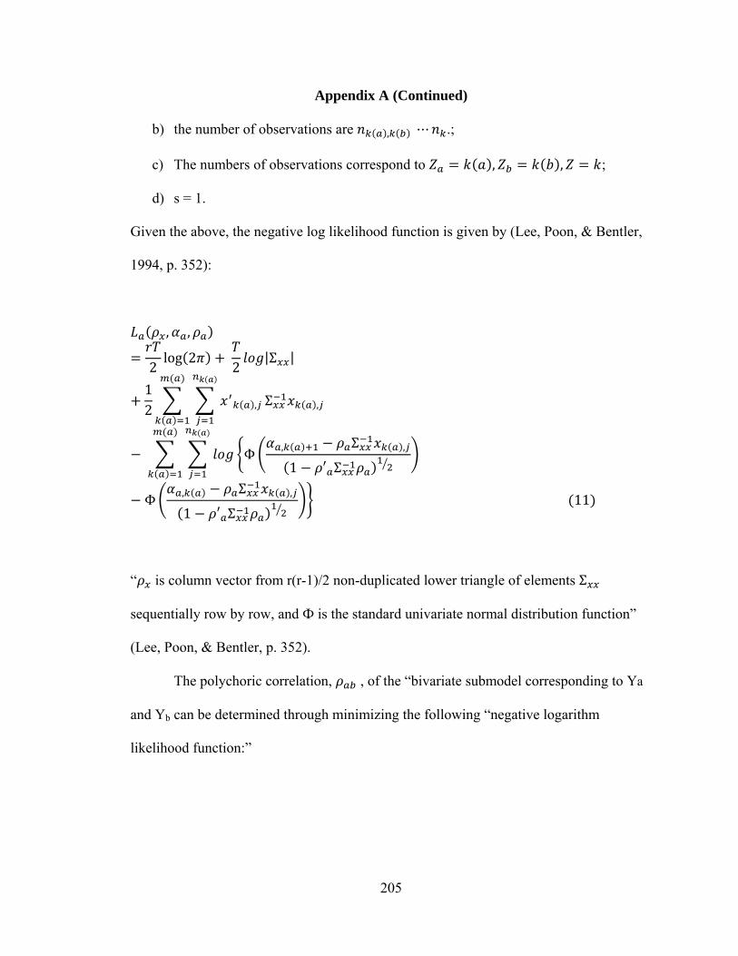
Appendix A (Continued)
205
b) the number of observations are , ⋯ .;
c) The numbers of observations correspond to , , ;
d) s = 1.
Given the above, the negative log likelihood function is given by (Lee, Poon, & Bentler,
1994, p. 352):
, ,
2log 2
2|Σ |
12 , Σ ,
Φ , Σ ,
1 ′ Σ
Φ , Σ ,
1 ′ Σ 11
“ is column vector from r(r-1)/2 non-duplicated lower triangle of elements Σ
sequentially row by row, and Ф is the standard univariate normal distribution function”
(Lee, Poon, & Bentler, p. 352).
The polychoric correlation, , of the “bivariate submodel corresponding to Ya
and Yb can be determined through minimizing the following “negative logarithm
likelihood function:”

Appendix A (Continued)
206
, ,
, ,
12
Where “. . . {k(a), k(b)} are respectively the ath and bth element of an observation zk in
the s dimensional sample space” (Lee, Poon, & Bentler, 1994, p. 353).
Because each random observation in the bivariate submodel corresponds to an
observation in the multivariate model, the negative logarithm likelihood function can be
simplified to:
, ,
, 13
In this maximum likelihood model, , , ′ is the vector that minimizes
, , (Poon, Lee, & Bentler, 1994).
Principal Axis Factor Analysis
If R is a correlation matrix with either communality estimates or ones on the main
diagonal, the following relationship can be defined (Cureton & D’Agostino, 1983):
(14)
Where:
a) The matrix E satisfies the condition that ;
b) the columns of E are eigenvectors for R;

Appendix A (Continued)
207
c) D is a diagonal matrix; the elements of the main diagonal of D are eigenvalues of
R
Because the above relationship holds “under permutations of the diagonal elements of D,
with corresponding permutations of the columns of E and the rows of E’,” the elements
of D are arranged in descending order (Cureton & D’Agostino, 1983, p. 143).
If R is of rank m < n, then D is a diagonal matrix containing zeroes in the last n -
m elements; the last n – m rows of E also consists of zeroes (Cureton & D’Agostino,
1983). The symmetric, matrix D can be written as:
(15)
Because D1/2 contains diagonal elements , R can be written as (Cureton &
D’Agostino, 1983; Harman, 1976):
(16)
A Gramian matrix is symmetric and includes only real numbers among its
elements. A Gramian (B) matrix must also have another real matrix (A) that when
multiplied by its transpose yields the original matrix. Formally, this relationship is
defined as (Cureton & D’Agostino, 1983; Harman, 1976):
(17)
When R is a Grammian, correlation matrix with communality estimates in the main
diagonal, then the trace of the matrix is equal to the sum of its eigenvalues. The
relationship between the principal-axes of factor loadings (F) and the reduced correlation
matrix is defined as (Cureton & D’Agostino, 1983):
(18)

Appendix A (Continued)
208
From the above consideration, then the matrix F can be defined as (Cureton &
D’Agostino, 1983):
(19)
The trace of R is equal to the sum of its eigenvalues. The sum of the squared
elements of F is equal to the eigenvalues for that column. The relationship between the
matrix of factor loadings and eigenvalues can be written as (Cureton & D’Agostino,
1983):
(20)
According to the basic factor analysis model, the predicted value of a given
variable, in standardized form, can be given by (Cureton & D’Agostino, 1983; Harman,
1976):
… … 1, 2, … (21)
Where the observed variables, j, are described in terms of m common factors, F. The
value of a given variable for an individual is given by (Cureton & D’Agostino, 1983;
Harman, 1976):
1, 2, … ; 1, 2 … 22
In this equation,
a) is the value of the common factor for individual ;
b) represents the residual error;
c) represents the contribution of a specific factor, , to the value of
(Harman, 1976, p. 15).
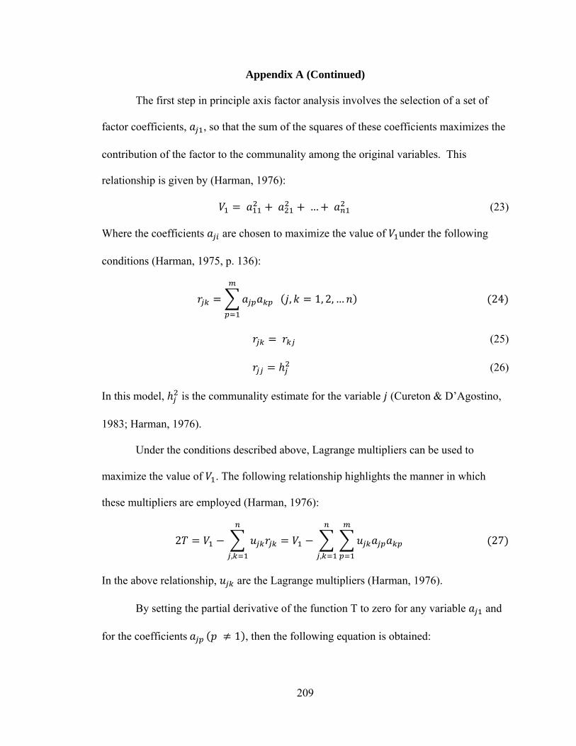
Appendix A (Continued)
209
The first step in principle axis factor analysis involves the selection of a set of
factor coefficients, , so that the sum of the squares of these coefficients maximizes the
contribution of the factor to the communality among the original variables. This
relationship is given by (Harman, 1976):
… (23)
Where the coefficients are chosen to maximize the value of under the following
conditions (Harman, 1975, p. 136):
, 1, 2, … 24
(25)
(26)
In this model, is the communality estimate for the variable (Cureton & D’Agostino,
1983; Harman, 1976).
Under the conditions described above, Lagrange multipliers can be used to
maximize the value of . The following relationship highlights the manner in which
these multipliers are employed (Harman, 1976):
2,,
27
In the above relationship, are the Lagrange multipliers (Harman, 1976).
By setting the partial derivative of the function T to zero for any variable and
for the coefficients 1 , then the following equation is obtained:

Appendix A (Continued)
210
0 28
Where 1 if 1 and 0 if 1 (Harman, 1976, p. 136).
When the above equation is multiplied by and summed over j, the following
relationship results (Harman, 1976):
0 29
According to the above relationship:
30
Therefore, by setting
31
the above equation becomes
0 32
Under the condition that
, 1, 2, … 33
the last equation becomes (Harman, 1976):
0 34

Appendix A (Continued)
211
The above relationship leads to a set of equations for each value of ; this system of
equations can be written as (Harman, 1976):
⋯ 0 ⋯ 0 ⋯ 0
......... ......... ......... ⋯ 0
(35)
The maximization of “ . . . leads to the system of equations for the solution of the
unknowns .” For this system of equations to have a “non-trivial solution,” the
determinant of the coefficients of the must vanish (Harman, 1976, p. 137). The
following relationship illustrates this condition:
⋯⋯⋯
⋯ ⋯ ⋯ ⋯ ⋯⋯
0 (36)
The above equation, in “determinantal form,” is a characteristic equation. The roots of
this equation are real, and, when substituted for , these roots reduce the rank of the
determinant to . From these considerations, the value of V can be defined as:
37
Therefore, is the largest root of the characteristic equation (Cureton & D’Agostino,
1983; Harman, 1976). The characteristic root is also referred to as an eigenvalue, and
this allows for the identification of coefficients of the first factor that account for the

Appendix A (Continued)
212
largest amount of the total communality possible (Cureton & D’Agostino, 1983; Harman,
1976).
The pattern of factor coefficients for the first factor is determined by:
√⋯
1, 2, … , (38)
The set ′ are solutions to the equations for values of . This vector is called an
eigenvector (Cureton & D’Agostino, 1983; Harman, 1976).
Once the set of factor coefficients for the first factor are determined, finding a
factor that accounts for the maximum amount of residual communality becomes the next
step in the factor analytic process (Cureton & D’Agostino, 1983; Harman, 1976). The
matrix of first factor residuals is defined as:
(39)
Where
(40)
This is an matrix of the products of the first factor coefficients (Harman, 1976).
By maximizing the value of , the the coefficients for the second factor, , are
determined. This value is given by:
⋯ (41)
The maximum value of the root of the first factor residuals is the second largest root of
the original correlation matrix (Cureton & D’Agostino, 1983; Harman, 1976). By this
process, the eigenvalues and associated eigenvectors are derived from the original

Appendix A (Continued)
213
correlation matrix until factors are extracted (Cureton & D’Agostino, 1983; Harman,
1976).
Ordinary Least Squares Factor Analysis
In Ordinary Least Squares factor analysis, the relationship between factor pattern
matrices, A, and implied correlation matrices, , is given by (Cureton & D’Agostino,
1983; Harman, 1976):
(42)
The least squares solution can be found by “fitting by ”
(Harman, 1976, p. 176).
Where
(43)
The diagonal matrix described in equation 43 contains communalities. Minimizing the
off-diagonal residuals results in the ordinary least squares method for developing factor
solutions (Cureton & D’Agostino, 1983; Harman, 1976). This minimization is given by
the following expression (Harman, 1976):
min (44)
The function to be minimized can be written algebraically as:
45
Through varying the values of factor loadings, the objective is to minimize this function
for a specified number of factors, m (Harman, 1976). To develop a function that is
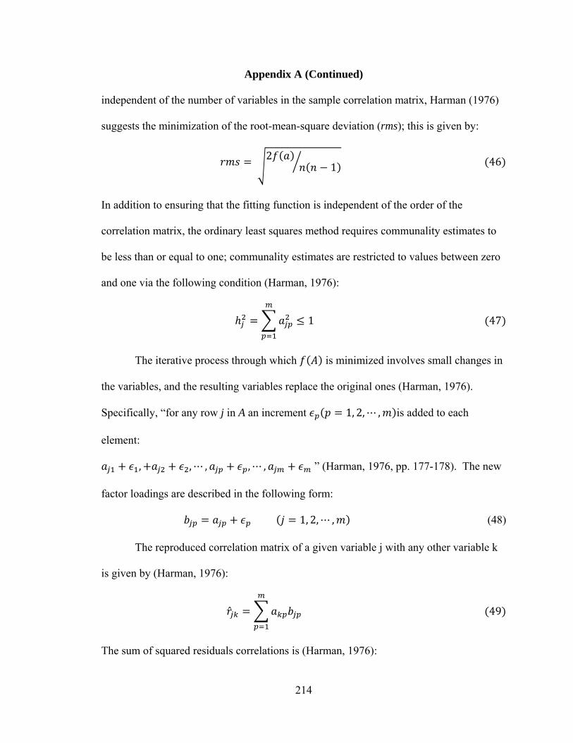
Appendix A (Continued)
214
independent of the number of variables in the sample correlation matrix, Harman (1976)
suggests the minimization of the root-mean-square deviation (rms); this is given by:
21 46
In addition to ensuring that the fitting function is independent of the order of the
correlation matrix, the ordinary least squares method requires communality estimates to
be less than or equal to one; communality estimates are restricted to values between zero
and one via the following condition (Harman, 1976):
1 47
The iterative process through which is minimized involves small changes in
the variables, and the resulting variables replace the original ones (Harman, 1976).
Specifically, “for any row j in A an increment 1, 2,⋯ , is added to each
element:
, , ⋯ , ,⋯ , ” (Harman, 1976, pp. 177-178). The new
factor loadings are described in the following form:
1, 2,⋯ , (48)
The reproduced correlation matrix of a given variable j with any other variable k
is given by (Harman, 1976):
49
The sum of squared residuals correlations is (Harman, 1976):

Appendix A (Continued)
215
50
When the original factor loading is “separated from the incremental change,” the above
equation becomes (Harman, 1976, p. 178):
∗ 51
With the incremental changes in factor loadings removed, the original residual
correlations, ∗ , of variables k with a fixed j are given by (Harman, 1976):
∗ 1, 2,⋯ , ; 52
The first step in determining the values of that minimize the function involves taking
the partial derivatives of the sum of squared residual correlations with the original factor
loadings separated from the incremental changes; this expression becomes:
2 ∗ 1, 2,⋯ , 53
In the second step, these equations are set to zero; this leads to the following “implicit
equations” (Harman, 1976, p. 178):
∗ 1, 2,⋯ , 54

Appendix A (Continued)
216
, , ⋯ , (55)
In this expression,
a) is a row vector of incremental changes of the factor loadings for variable ;
b) is the factor loading matrix with the elements in row replaced with zeros;
c) is the row vector of residual correlations of with all other variables.
The solution for the values of that minimize the function is given by (Harman,
1976):
(56)
In ordinary least squares, Heywood cases, or factor solutions that imply
communalities greater than one, are not considered proper solutions. Therefore, when
solutions that minimize the function result in communalities that are greater than one,
the following constraint is applied (Harman, 1976):
1 57
This constraint ensures that minimum values of the fitting function yield proper factor
solutions.
Maximum Likelihood Factor Analysis
Before using a maximum likelihood strategy to develop estimates of common
factor loadings, a researcher must first use sample data to create a distribution of the
elements of a covariance matrix. When samples of observations are drawn from
multivariate normal distributions, the distribution function of the elements of the
covariance matrix can be defined as (Harman, 1976):
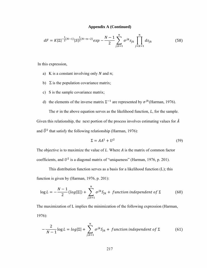
Appendix A (Continued)
217
|Σ| | |1
2,
58
In this expression,
a) K is a constant involving only and ;
b) is the population covariance matrix;
c) S is the sample covariance matrix;
d) the elements of the inverse matrix Σ are represented by (Harman, 1976).
The in the above equation serves as the likelihood function, , for the sample.
Given this relationship, the next portion of the process involves estimating values for
and that satisfy the following relationship (Harman, 1976):
Σ (59)
The objective is to maximize the value of . Where is the matrix of common factor
coefficients, and is a diagonal matrix of “uniqueness” (Harman, 1976, p. 201).
This distribution function serves as a basis for a likelihood function (L); this
function is given by (Harman, 1976, p. 201):
log1
2|Σ| Σ
,
60
The maximization of L implies the minimization of the following expression (Harman,
1976):
2 1
log |Σ| Σ,
61

Appendix A (Continued)
218
The next step in the maximum likelihood estimation process involves finding the
partial derivatives with respect to and and equating these expressions to zero; these
calculations include “ variables in all.” Because the “estimated factor loadings for
each variable are proportional the standard deviation of that variable,” the estimation
equations are scale independent (Harman, 1976, p. 201). The following equations present
the results of the estimation procedures in matrix form (Harman, 1976):
Ρ (62)
Ρ (63)
(64)
(65)
Where Ρ is the population correlation matrix, Ρ is an estimator of the population
correlation matrix, and R is the sample correlation matrix with ones on the main diagonal
(Harman, 1976).
Although the process described above will provide a basis for developing
maximum likelihood estimates of factor loadings, Harman (1976) suggests assuming an
equivalency between the sample correlation matrix and the estimator of the population
correlation matrix. This assumption yields a simpler process for obtaining factor loading
estimates. The expression for can be rewritten as (Harman, 1976):
(66)
The following expression results from premultiplying both sides of the equation by
:
(67)
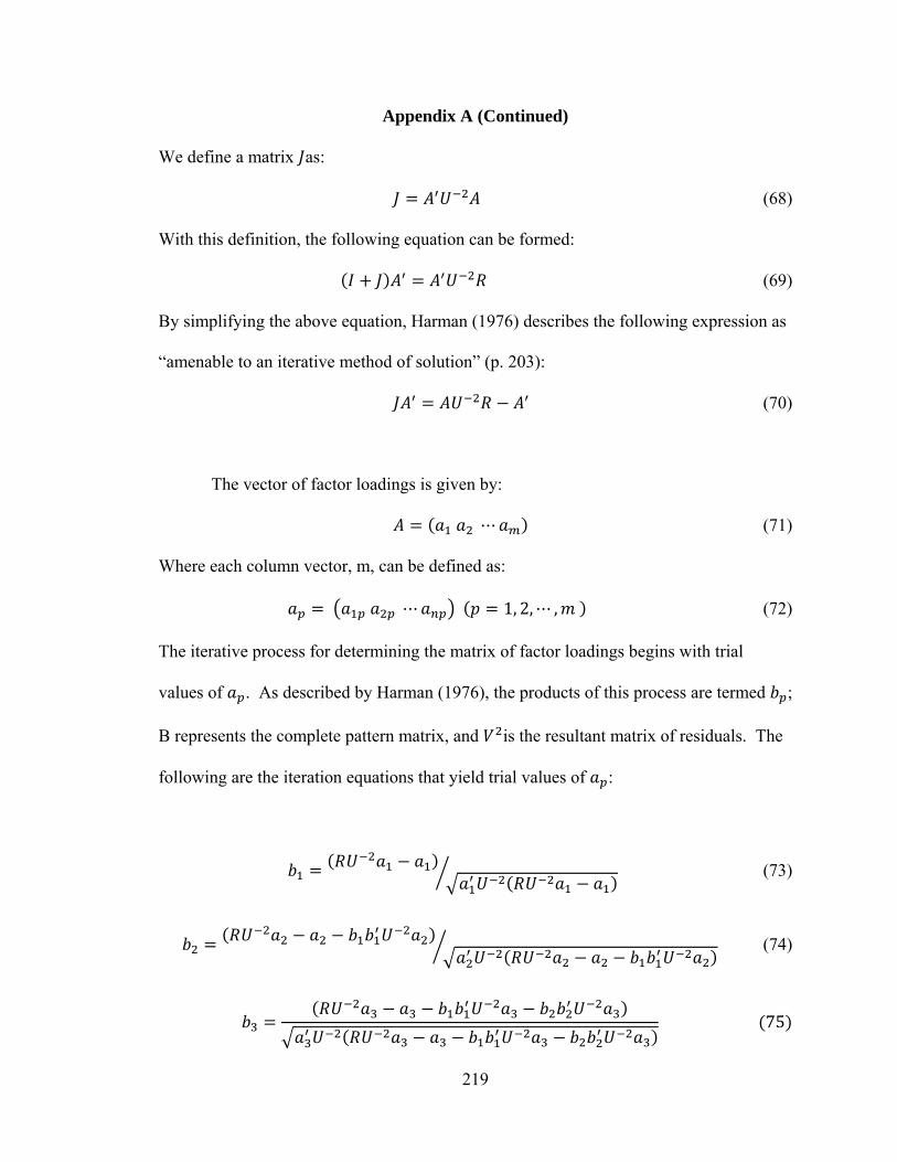
Appendix A (Continued)
219
We define a matrix as:
(68)
With this definition, the following equation can be formed:
(69)
By simplifying the above equation, Harman (1976) describes the following expression as
“amenable to an iterative method of solution” (p. 203):
(70)
The vector of factor loadings is given by:
⋯ (71)
Where each column vector, m, can be defined as:
⋯ 1, 2,⋯ , (72)
The iterative process for determining the matrix of factor loadings begins with trial
values of . As described by Harman (1976), the products of this process are termed ;
B represents the complete pattern matrix, and is the resultant matrix of residuals. The
following are the iteration equations that yield trial values of :
(73)
(74)
75

Appendix A (Continued)
220
(76)
While the above equations illustrate a three factor pattern, the process can be
generalized to any number of factors (Harman, 1976). This process is repeated until the
algorithm converges on a solution, a matrix that fulfills a prescribed degree of closeness.
The resulting matrix, A, contains maximum likelihood estimates of factor loadings
(Harman, 1976).
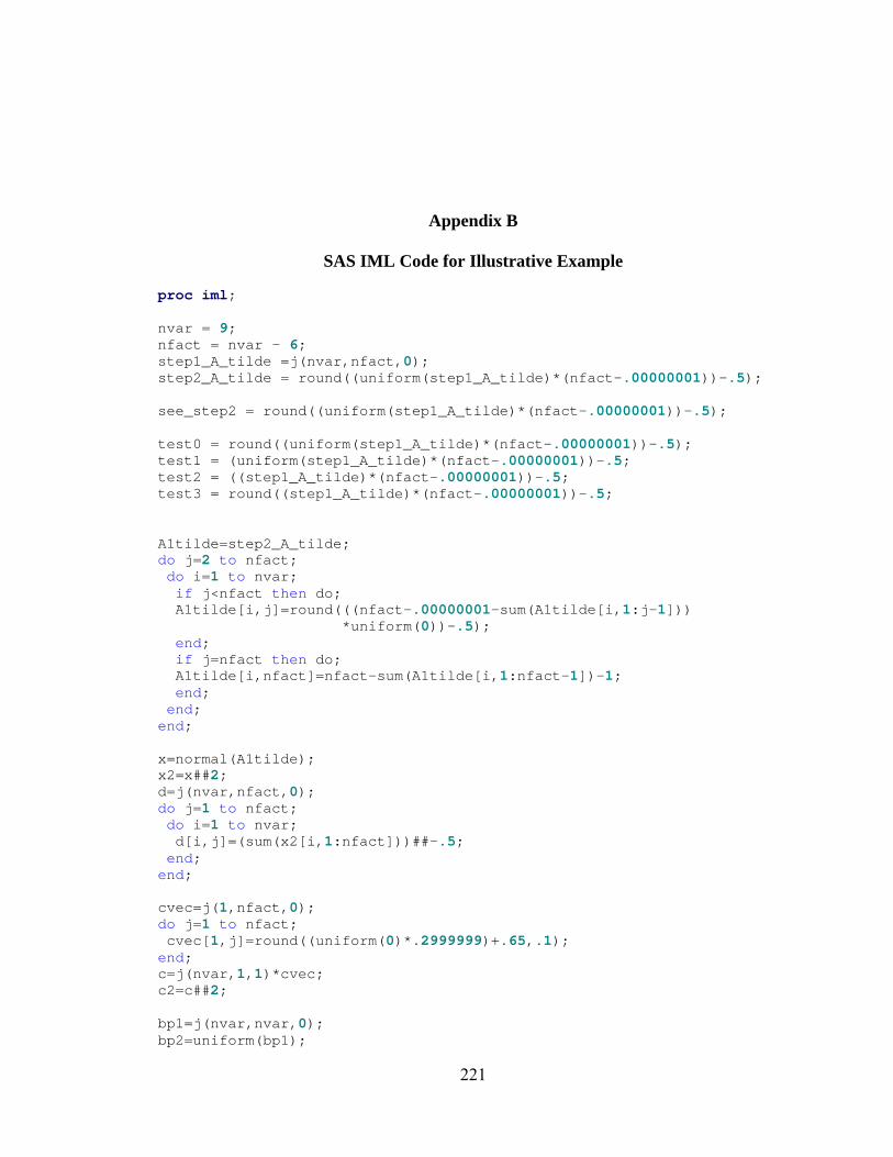
Appendix B
221
SAS IML Code for Illustrative Example proc iml; nvar = 9; nfact = nvar - 6; step1_A_tilde =j(nvar,nfact,0); step2_A_tilde = round((uniform(step1_A_tilde)*(nfact-.00000001))-.5); see_step2 = round((uniform(step1_A_tilde)*(nfact-.00000001))-.5); test0 = round((uniform(step1_A_tilde)*(nfact-.00000001))-.5); test1 = (uniform(step1_A_tilde)*(nfact-.00000001))-.5; test2 = ((step1_A_tilde)*(nfact-.00000001))-.5; test3 = round((step1_A_tilde)*(nfact-.00000001))-.5; A1tilde=step2_A_tilde; do j=2 to nfact; do i=1 to nvar; if j<nfact then do; A1tilde[i,j]=round(((nfact-.00000001-sum(A1tilde[i,1:j-1])) *uniform(0))-.5); end; if j=nfact then do; A1tilde[i,nfact]=nfact-sum(A1tilde[i,1:nfact-1])-1; end; end; end; x=normal(A1tilde); x2=x##2; d=j(nvar,nfact,0); do j=1 to nfact; do i=1 to nvar; d[i,j]=(sum(x2[i,1:nfact]))##-.5; end; end; cvec=j(1,nfact,0); do j=1 to nfact; cvec[1,j]=round((uniform(0)*.2999999)+.65,.1); end; c=j(nvar,1,1)*cvec; c2=c##2; bp1=j(nvar,nvar,0); bp2=uniform(bp1);
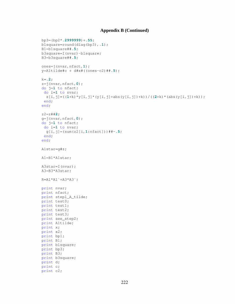
Appendix B (Continued)
222
bp3=(bp2*.2999999)+.55; b1square=round(diag(bp3),.1); B1=b1square##.5; b3square=I(nvar)-b1square; B3=b3square##.5; ones=j(nvar,nfact,1); y=A1tilde#c + d#x#((ones-c2)##.5); k=.2; z=j(nvar,nfact,0); do j=1 to nfact; do i=1 to nvar; z[i,j]=((1+k)*y[i,j]*(y[i,j]+abs(y[i,j])+k))/((2+k)*(abs(y[i,j])+k)); end; end; z2=z##2; g=j(nvar,nfact,0); do j=1 to nfact; do i=1 to nvar; g[i,j]=(sum(z2[i,1:nfact]))##-.5; end; end; A1star=g#z; A1=B1*A1star; A3star=I(nvar); A3=B3*A3star; R=A1*A1`+A3*A3`; print nvar; print nfact; print step1_A_tilde; print test0; print test1; print test2; print test3; print see_step2; print A1tilde; print x; print x2; print bp1; print B1; print b1square; print bp3; print B3; print b3square; print d; print c; print c2;

Appendix B (Continued)
223
print y; print z; print A1star; print A1; print A3star; print A3; print R; quit;
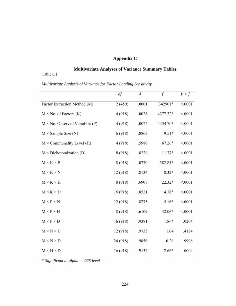
Appendix C
224
Multivariate Analyses of Variance Summary Tables Table C1
Multivariate Analysis of Variance for Factor Loading Sensitivity
df f P > f
Factor Extraction Method (M) 2 (459) .0001 342901* <.0001
M × No. of Factors (K) 4 (918) .0026 4277.32* <.0001
M × No. Observed Variables (P) 4 (918) .0024 4454.70* <.0001
M × Sample Size (N) 6 (918) .8863 9.51* <.0001
M × Communality Level (H) 4 (918) .5980 67.26* <.0001
M × Dichotomization (D) 8 (918) .8226 11.77* <.0001
M × K × P 8 (918) .0270 582.84* <.0001
M × K × N 12 (918) .8134 8.32* <.0001
M × K × H 8 (918) .6907 22.32* <.0001
M × K × D 16 (918) .8521 4.78* <.0001
M × P × N 12 (918) .8775 5.16* <.0001
M × P × H 8 (918) .6109 32.06* <.0001
M × P × D 16 (918) .9381 1.86* .0204
M × N × H 12 (918) .9735 1.04 .4134
M × N × D 24 (918) .9856 0.28 .9998
M × H × D 16 (918) .9134 2.66* .0004
* Significant at alpha = .025 level

Appendix C (Continued)
225
Table C2
Repeated Measures Analysis of Variance for Factor Loading Sensitivity
Source df SS MS F P
Between Subjects
Number of Factors (K) 2 26.477 13.239 34780.8* <.0001 .999
Number of Variables (P) 2 41.680 20.840 54751.0* <.0001 .993
Sample Size (N) 3 0.012 0.004 10.96* <.0001 .044
Communality (H) 2 0.142 0.071 186.45* <.0001 .343
Dichotomization (D) 4 0.027 0.007 17.86* <.0001 .091
K × P 4 1.693 0.423 1111.93* <.0001 .862
K × N 6 0.003 0.0005 1.42 .205 .011
K × H 4 0.018 0.004 11.81* <.0001 .062
K × D 8 0.016 0.002 5.43* <.0001 .574
P × N 6 0.003 0.0006 1.51 .174 .012
P × H 4 0.216 0.005 14.21* <.0001 .074
P × D 8 0.004 0.0005 1.38 .204 .015
N × H 6 0.001 0.0002 0.55 .770 .004
N × D 12 0.002 0.0001 0.38 .969 .006
H × D 8 0.10 0.001 3.41* .001 .037
Error 460 0.175 0.0003
Appendix C (Continued)
226
Table C2
Repeated Measures Analysis of Variance for Factor Loading Sensitivity (Continued)
Source df SS MS F P
Within Subjects (with Greenhouse-Geisser asjusted Pr > F)
Factor Extraction Method (M) 2 125.806 62.903 600815* <.0001 .998
M × K 4 13.599 3.400 32474.6* <.0001 .980
M × P 4 20.986 5.246 50111.1* <.0001 .987
M × N 6 0.003 0.0005 4.42* .0019 .010
M × H 4 0.018 0.005 44.39* <.0001 .064
M × D 8 0.014 0.0018 16.81* <.0001 .049
M × K × P 8 0.910 0.114 1086.34* <.0001 .770
M × K × N 12 0.009 0.0008 7.48* <.0001 .033
M × K × H 8 0.011 0.0014 13.09* <.0001 .038
M × K × D 16 0.010 0.0006 5.75* <.0001 .034
M × P × N 12 0.003 0.0002 2.21 .0269 .010
M × P × H 8 0.0171 0.0020 20.47* <.0001 .059
M × P × D 16 0.003 0.0002 1.74 .0663 .011
M × N × H 12 0.001 0.0001 1.16 .325 .005
Appendix C (Continued)
227
Table C3
Multivariate Analysis of Variance for General Pattern Agreement Values
df f P > f
Factor Extraction Method (M) 2 (459) .0020 109246* <.0001
M × No. of Factors (K) 4 (918) .0349 997.42* <.0001
M × No. Observed Variables (P) 4 (918) .0235 1267.08* <.0001
M × Sample Size (N) 6 (918) .3531 104.48* <.0001
M × Communality Level (H) 4 (918) .0962 540.34* <.0001
M × Dichotomization (D) 8 (918) .9779 1.29 .2451
M × K × P 8 (918) .2009 141.24* <.0001
M × K × N 12 (918) .7233 13.45* <.0001
M × K × H 8 (918) .3087 91.78* <.0001
M × K × D 16 (918) .9242 2.31* .0025
M × P × N 12 (918) .9455 2.17* .0113
M × P × H 8 (918) .7637 16.56* <.0001
M × P × D 16 (918) .9718 0.15 .6554
M × N × H 12 (918) .5289 28.99* <.0001
M × N × D 24 (918) .9920 0.15 1.0000
M × H × D 16 (918) .9819 0.53 .9343
* Significant at alpha = .025 level

Appendix C (Continued)
228
Table C4
Repeated Measures Analysis of Variance for General Pattern Agreement
Source Df SS MS F P
Between Subjects
Number of Factors (K) 2 3.356 1.678 1053.97* <.0001 .764
Number of Variables (P) 2 9.830 4.915 3087.36* <.0001 .904
Sample Size (N) 3 0.547 0.182 114.48* <.0001 .345
Communality (H) 2 4.040 2.020 1268.82* <.0001 .795
Dichotomization (D) 4 0.018 0.005 2.98* .0191 .018
K × P 4 5.067 1.267 795.69* <.0001 .830
K × N 6 0.100 0.0167 10.51* <.0001 .088
K × H 4 0.877 0.219 137.80* <.0001 .458
K × D 8 .034 0.004 2.67* .0072 .032
P × N 6 0.006 0.001 0.66 .6793 .006
P × H 4 0.583 0.146 91.50* <.0001 .359
P × D 8 0.018 0.002 1.43 .1799 .017
N × H 6 0.033 0.005 3.51* .0021 .031
N × D 12 0.002 0.000 0.09 1.00 .001
H × D 8 0.004 0.005 0.33 .9549 .004
Error 460 0.732 0.001

Appendix C (Continued)
229
Table C4
Repeated Measures Analysis of Variance for General Pattern Agreement (Continued)
Source Df SS MS F P
Within Subjects (with Greenhouse-Geisser asjusted Pr > F)
Factor Extraction Method (M) 2 128.078 64.039 192576* <.0001 .991
M × K 4 4.695 1.174 3529.54* <.0001 .819
M × P 4 11.741 2.935 8826.69* <.0001 .919
M × N 6 0.403 0.067 201.90* <.0001 .280
M × H 4 2.414 0.603 1814.89* <.0001 .699
M × D 8 0.003 0.000 0.99 .4209 .002
M × K × P 8 0.758 0.095 284.98* <.0001 .422
M × K × N 12 0.026 0.002 6.50* <.0001 .024
M × K × H 8 0.504 0.063 189.60* <.0001 .327
M × K × D 16 0.184 0.001 3.47* .0003 .017
M × P × N 12 0.011 0.001 2.80* .0078 .011
M × P × H 8 0.022 0.003 8.49* <.0001 .021
M × P × D 16 0.007 0.000 1.38 .1950 .007
M × N × H 12 0.229 0.019 57.33* <.0001 .180
M × N × D 24 0.001 0.000 0.10 1.000 .001
M × H × D 16 0.004 0.000 0.71 .6973 .003
Error (Method) 920 0.306 0.000
* Significant at the alpha = .025 level
Appendix C (Continued)
230
Table C5
Multivariate Analysis of Variance for Per Element Pattern Agreement
df Λ f P > f
Factor Extraction Method (M) 2 (459) .0085 26828.4* <.0001
M × No. of Factors (K) 4 (918) .0157 1599.46* <.0001
M × No. Observed Variables (P) 4 (918) .0888 540.51* <.0001
M × Sample Size (N) 6 (918) .3154 119.42* <.0001
M × Communality Level (H) 4 (918) .1318 402.65* <.0001
M × Dichotomization (D) 8 (918) .9611 2.30* .0192
M × K × P 8 (918) .1220 213.70* <.0001
M × K × N 12 (918) .7942 9.34* <.0001
M × K × H 8 (918) .6730 25.12* <.0001
M × K × D 16 (918) .8355 5.39* <.0001
M × P × N 12 (918) .8618 5.91* <.0001
M × P × H 8 (918) .6102 32.14* <.0001
M × P × D 16 (918) .9431 1.71 .0403
M × N × H 12 (918) .5823 23.75* <.0001
M × N × D 24 (918) .9940 0.12 1.0000
M × H × D 16 (918) 0.9336 2.00* .0107
* Significant at alpha = .025 level

Appendix C (Continued)
231
Table C6
Repeated Measures Analysis of Variance for Per Element Pattern Agreement
Source Df SS MS F P
Between Subjects
Number of Factors (K) 2 26.148 13.074 12137.8* <.0001 .978
Number of Variables (P) 2 0.285 0.142 132.18* <.0001 .330
Sample Size (N) 3 0.338 0.113 104.67* <.0001 .370
Communality (H) 2 1.293 0.646 600.08* <.0001 .691
Dichotomization (D) 4 0.017 0.004 4.01* .0033 .029
K × P 4 3.874 0.968 899.10* <.0001 .870
K × N 6 0.120 0.020 18.540* <.0001 .172
K × H 4 0.417 0.104 96.70* <.0001 .419
K × D 8 0.035 0.004 4.07* .0001 .057
P × N 6 0.027 0.004 4.16* .0004 .044
P × H 4 0.106 0.026 25.54* <.0001 .155
P × D 8 0.030 0.004 3.43* .0007 .049
N × H 6 0.059 0.010 9.10* <.0001 .092
N × D 12 0.001 0.000 0.05 1.000 .001
H × D 8 0.020 0.002 2.33* 0.019 .033
Error 460 0.495 0.001

Appendix C (Continued)
232
Table C6
Repeated Measures Analysis of Variance for Per Element Pattern Agreement (Continued)
Source Df SS MS F P
Within Subjects (with Greenhouse-Geisser asjusted Pr > F)
Factor Extraction Method (M) 2 8.235 4.118 45801.9* <.0001 .934
M × K 4 4.122 1.030 11461.9* <.0001 .877
M × P 4 0.641 0.160 1781.58* <.0001 .526
M × N 6 0.140 0.233 259.35* <.0001 .195
M × H 4 0.438 0.109 1219.6* <.0001 .431
M × D 8 0.002 0.000 2.86* .0178 .003
M × K × P 8 0.521 0.065 724.05* <.0001 .474
M × K × N 12 0.003 0.000 2.67* .0100 .004
M × K × H 8 0.028 0.003 38.25* <.0001 .045
M × K × D 16 0.121 0.001 8.43* <.0001 .020
M × P × N 12 0.002 0.000 1.96 .0622 .004
M × P × H 8 0.018 0.002 24.36* <.0001 .029
M × P × D 16 0.003 0.000 2.14* .0226 .005
M × N × H 12 0.048 0.004 44.65* <.0001 .077
M × N × D 24 0.000 0.000 0.09 1.0000 .000
M × H × D 16 0.004 0.000 3.13* .0009 .007
Error (Method) 920 0.083 0.000
* Significant at the alpha = .025 level

Appendix C (Continued)
233
Table C7
Multivariate Analysis of Variance Summary for Total Pattern Agreement
Df f P > f
Factor Extraction Method (M) 2 (459) .7290 85.36* <.0001
M × No. of Factors (K) 4 (918) .5764 72.79* <.0001
M × No. Observed Variables (P) 4 (918) .6269 60.35* <.0001
M × Sample Size (N) 6 (918) .9184 6.65* <.0001
M × Communality Level (H) 4 (918) .9806 2.26 .0609
M × Dichotomization (D) 8 (918) .9541 2.73* .0057
M × K × P 8 (918) .4592 54.59* <.0001
M × K × N 12 (918) .8543 6.27* <.0001
M × K × H 8 (918) .9592 2.41 .0141
M × K × D 16 (918) .9094 2.79* .0002
M × P × N 12 (918) .8778 5.15* <.0001
M × P × H 8 (918) .9683 1.86 .0626
M × P × D 16 (918) .9250 2.28* .0028
M × N × H 12 (918) .9856 0.56 .8782
M × N × D 24 (918) .9679 0.63 .9165
M × H × D 16 (918) .9455 1.63 .0552
* Significant at alpha = .025 level
Appendix C (Continued)
234
Table C8
Repeated Measures Analysis of Variance for Total Pattern Agreement
Source Df SS MS F P
Between Subjects
Number of Factors (K) 2 <.0001 <.0001 167.05* <.0001 .195
Number of Variables (P) 2 <.0001 <.0001 136.36* <.0001 .165
Sample Size (N) 3 <.0001 <.0001 12.55* <.0001 .026
Communality (H) 2 <.0001 <.0001 3.12 .0321 .005
Dichotomization (D) 4 <.0001 <.0001 4.49* .0015 .013
K × P 4 <.0001 <.0001 133.20* <.0001 .278
K × N 6 <.0001 <.0001 11.90* <.0001 .049
K × H 4 <.0001 <.0001 3.90* .0040 .011
K × D 8 <.0001 <.0001 4.64* <.0001 .026
P × N 6 <.0001 <.0001 9.56* <.0001 .040
P × H 4 <.0001 <.0001 2.68 .0311 .008
P × D 8 <.0001 <.0001 3.59* .0005 .020
N × H 6 <.0001 <.0001 0.12 .9943 .000
N × D 12 <.0001 <.0001 0.25 .9945 .002
H × D 8 <.0001 <.0001 2.27* .0220 .013
Error 460 <.0001 <.0001

Appendix C (Continued)
235
Table C8
Repeated Measures Analysis of Variance for Total Pattern Agreement (Continued)
Source Df SS MS F P
Within Subjects (with Greenhouse-Geisser asjusted Pr > F)
Factor Extraction Method (M) 2 <.0001 <.0001 170.43* <.0001 .198
M × K 4 <.0001 <.0001 167.25* <.0001 .326
M × P 4 <.0001 <.0001 136.17* <.0001 .283
M × N 6 <.0001 <.0001 12.55* <.0001 .052
M × H 4 <.0001 <.0001 3.50 .0310 .010
M × D 8 <.0001 <.0001 4.49* .0014 .025
M × K × P 8 <.0001 <.0001 133.37* <.0001 .436
M × K × N 12 <.0001 <.0001 11.91* <.0001 .094
M × K × H 8 <.0001 <.0001 3.89* .0041 .022
M × K × D 16 <.0001 <.0001 4.64* <.0001 .051
M × P × N 12 <.0001 <.0001 9.56* <.0001 .077
M × P × H 8 <.0001 <.0001 2.71 .0295 .015
M × P × D 16 <.0001 <.0001 3.60* .0005 .040
M × N × H 12 <.0001 <.0001 0.12 .9944 .001
M × N × D 24 <.0001 <.0001 0.26 .9944 .004
M × H × D 16 <.0001 <.0001 2.27* .0217 .025
Error (Method) 920 .0001 <.0001
* Significant at the alpha = .025 level
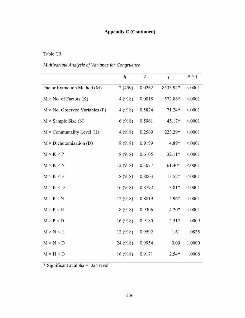
Appendix C (Continued)
236
Table C9
Multivariate Analysis of Variance for Congruence
df f P > f
Factor Extraction Method (M) 2 (459) 0.0262 8533.92* <.0001
M × No. of Factors (K) 4 (918) 0.0818 572.86* <.0001
M × No. Observed Variables (P) 4 (918) 0.5824 71.24* <.0001
M × Sample Size (N) 6 (918) 0.5961 45.17* <.0001
M × Communality Level (H) 4 (918) 0.2569 223.29* <.0001
M × Dichotomization (D) 8 (918) 0.9199 4.89* <.0001
M × K × P 8 (918) 0.6105 32.11* <.0001
M × K × N 12 (918) 0.3077 61.40* <.0001
M × K × H 8 (918) 0.8003 13.52* <.0001
M × K × D 16 (918) 0.8792 3.81* <.0001
M × P × N 12 (918) 0.8819 4.96* <.0001
M × P × H 8 (918) 0.9306 4.20* <.0001
M × P × D 16 (918) 0.9180 2.51* .0009
M × N × H 12 (918) 0.9592 1.61 .0835
M × N × D 24 (918) 0.9954 0.09 1.0000
M × H × D 16 (918) 0.9171 2.54* .0008
* Significant at alpha = .025 level
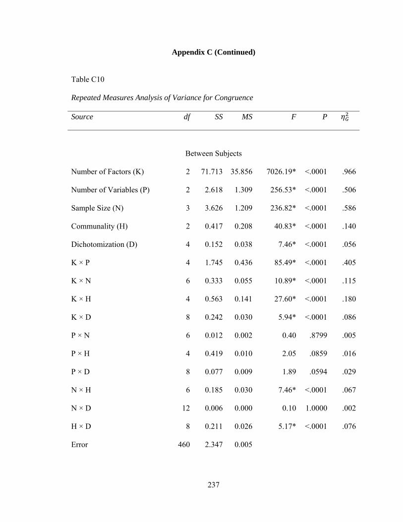
Appendix C (Continued)
237
Table C10
Repeated Measures Analysis of Variance for Congruence
Source df SS MS F P
Between Subjects
Number of Factors (K) 2 71.713 35.856 7026.19* <.0001 .966
Number of Variables (P) 2 2.618 1.309 256.53* <.0001 .506
Sample Size (N) 3 3.626 1.209 236.82* <.0001 .586
Communality (H) 2 0.417 0.208 40.83* <.0001 .140
Dichotomization (D) 4 0.152 0.038 7.46* <.0001 .056
K × P 4 1.745 0.436 85.49* <.0001 .405
K × N 6 0.333 0.055 10.89* <.0001 .115
K × H 4 0.563 0.141 27.60* <.0001 .180
K × D 8 0.242 0.030 5.94* <.0001 .086
P × N 6 0.012 0.002 0.40 .8799 .005
P × H 4 0.419 0.010 2.05 .0859 .016
P × D 8 0.077 0.009 1.89 .0594 .029
N × H 6 0.185 0.030 7.46* <.0001 .067
N × D 12 0.006 0.000 0.10 1.0000 .002
H × D 8 0.211 0.026 5.17* <.0001 .076
Error 460 2.347 0.005
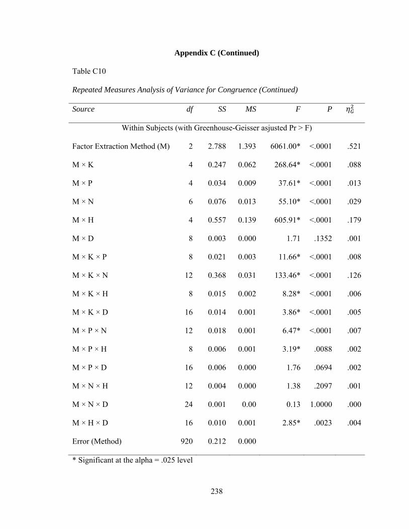
Appendix C (Continued)
238
Table C10
Repeated Measures Analysis of Variance for Congruence (Continued)
Source df SS MS F P
Within Subjects (with Greenhouse-Geisser asjusted Pr > F)
Factor Extraction Method (M) 2 2.788 1.393 6061.00* <.0001 .521
M × K 4 0.247 0.062 268.64* <.0001 .088
M × P 4 0.034 0.009 37.61* <.0001 .013
M × N 6 0.076 0.013 55.10* <.0001 .029
M × H 4 0.557 0.139 605.91* <.0001 .179
M × D 8 0.003 0.000 1.71 .1352 .001
M × K × P 8 0.021 0.003 11.66* <.0001 .008
M × K × N 12 0.368 0.031 133.46* <.0001 .126
M × K × H 8 0.015 0.002 8.28* <.0001 .006
M × K × D 16 0.014 0.001 3.86* <.0001 .005
M × P × N 12 0.018 0.001 6.47* <.0001 .007
M × P × H 8 0.006 0.001 3.19* .0088 .002
M × P × D 16 0.006 0.000 1.76 .0694 .002
M × N × H 12 0.004 0.000 1.38 .2097 .001
M × N × D 24 0.001 0.00 0.13 1.0000 .000
M × H × D 16 0.010 0.001 2.85* .0023 .004
Error (Method) 920 0.212 0.000
* Significant at the alpha = .025 level

Appendix C (Continued)
239
Table C11
Multivariate Analysis of Variance for Factor Score Correlations
df F P > f
Factor Extraction Method (M) 2 (400) .0218 8978.7* <.0001
M × No. of Factors (K) 4 (800) .0226 1129.49* <.0001
M × No. Observed Variables (P) 4 (800) .0698 556.90* <.0001
M × Sample Size (N) 6 (800) .5146 52.54* <.0001
M × Communality Level (H) 4 (800) .3978 117.08* <.0001
M × Dichotomization (D) 8 (800) .9486 2.67* .0067
M × K × P 6 (800) .0712 366.49* <.0001
M × K × N 12 (800) .6312 17.24* <.0001
M × K × H 8 (800) .6205 26.95* <.0001
M × K × D 16 (800) .9029 2.62* .0005
M × P × N 12 (800) .8982 3.67* <.0001
M × P × H 8 (800) .5600 33.63* <.0001
M × P × D 16 (800) .9544 1.18 .2777
M × N × H 12 (800) .9209 2.80* .0009
M × N × D 24 (800) .9917 0.14 1.0000
M × H × D 16 (800) .9704 0.76 .7346
* Significant at alpha = .025 level

Appendix C (Continued)
240
Table C12
Repeated Measures Analysis of Variance for Factor Score Correlations
Source df SS MS F P
Between Subjects
Number of Factors (K) 2 25.397 19.198 3046.54* <.0001 .924
Number of Variables (P) 2 3.278 1.639 378.36* <.0001 .601
Sample Size (N) 3 1.498 0.499 115.29* <.0001 .408
Communality (H) 2 0.414 0.207 47.75* <.0001 .160
Dichotomization (D) 4 0.019 0.005 1.08 .3666 .008
K × P 3 12.752 4.251 981.17* <.0001 .854
K × N 6 0.228 0.038 8.78* <.0001 .095
K × H 4 1.041 0.260 60.09* <.0001 .324
K × D 8 0.090 0.113 2.60* .0088 .040
P × N 6 0.019 0.003 0.74 .6208 .009
P × H 4 0.381 0.095 21.99* <.0001 .149
P × D 8 0.082 0.010 2.38* .0162 .037
N × H 6 0.113 0.019 4.34* .0003 .049
N × D 12 0.003 0.000 0.06 1.0000 .001
H × D 8 0.120 0.015 3.48* .0007 .053
Error 401 1.737 0.004
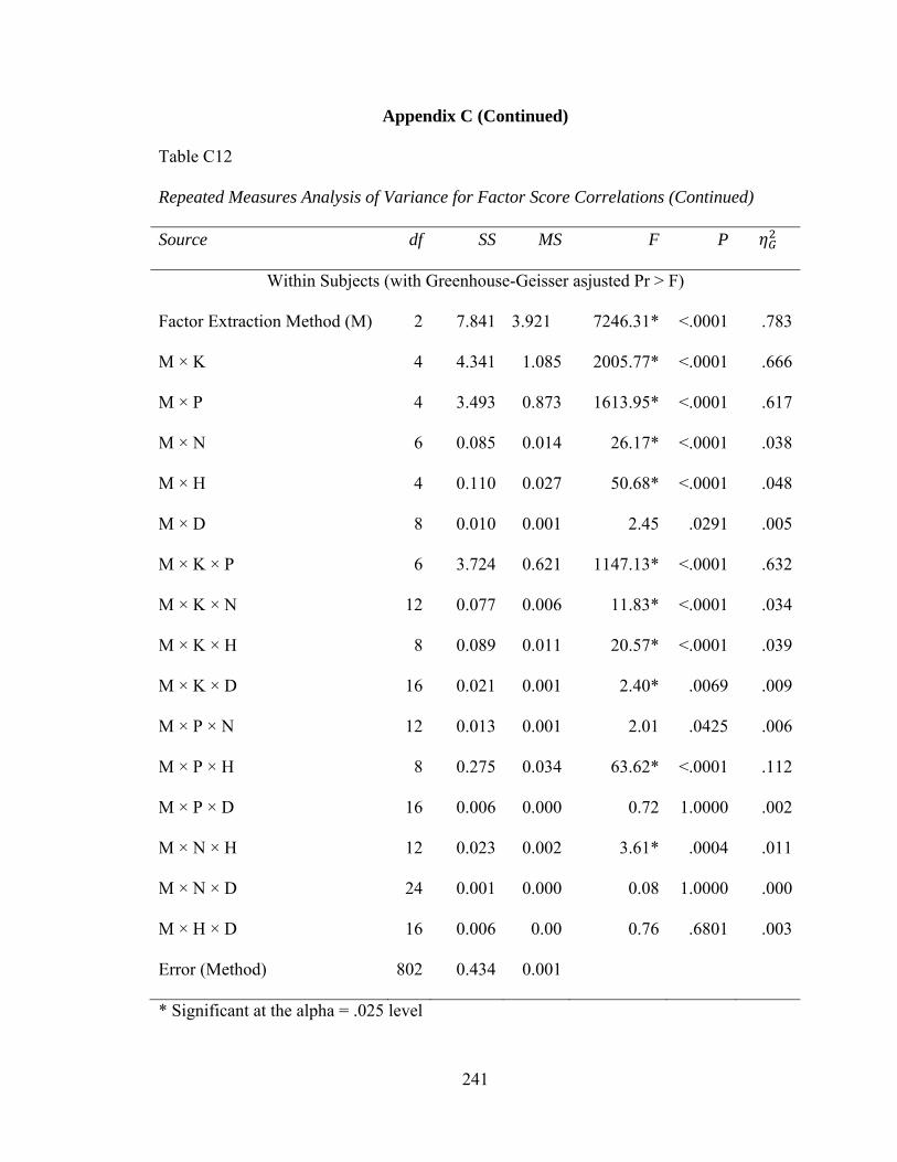
Appendix C (Continued)
241
Table C12
Repeated Measures Analysis of Variance for Factor Score Correlations (Continued)
Source df SS MS F P
Within Subjects (with Greenhouse-Geisser asjusted Pr > F)
Factor Extraction Method (M) 2 7.841 3.921 7246.31* <.0001 .783
M × K 4 4.341 1.085 2005.77* <.0001 .666
M × P 4 3.493 0.873 1613.95* <.0001 .617
M × N 6 0.085 0.014 26.17* <.0001 .038
M × H 4 0.110 0.027 50.68* <.0001 .048
M × D 8 0.010 0.001 2.45 .0291 .005
M × K × P 6 3.724 0.621 1147.13* <.0001 .632
M × K × N 12 0.077 0.006 11.83* <.0001 .034
M × K × H 8 0.089 0.011 20.57* <.0001 .039
M × K × D 16 0.021 0.001 2.40* .0069 .009
M × P × N 12 0.013 0.001 2.01 .0425 .006
M × P × H 8 0.275 0.034 63.62* <.0001 .112
M × P × D 16 0.006 0.000 0.72 1.0000 .002
M × N × H 12 0.023 0.002 3.61* .0004 .011
M × N × D 24 0.001 0.000 0.08 1.0000 .000
M × H × D 16 0.006 0.00 0.76 .6801 .003
Error (Method) 802 0.434 0.001
* Significant at the alpha = .025 level
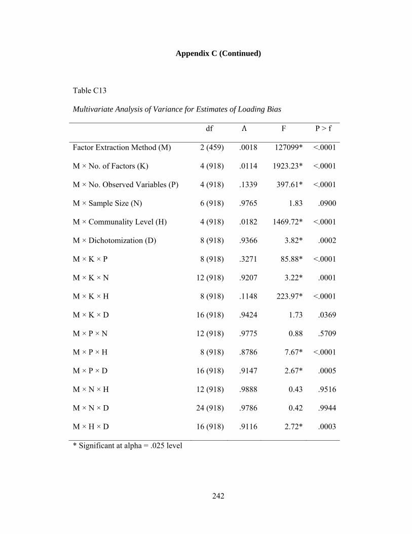
Appendix C (Continued)
242
Table C13
Multivariate Analysis of Variance for Estimates of Loading Bias
df Λ F P > f
Factor Extraction Method (M) 2 (459) .0018 127099* <.0001
M × No. of Factors (K) 4 (918) .0114 1923.23* <.0001
M × No. Observed Variables (P) 4 (918) .1339 397.61* <.0001
M × Sample Size (N) 6 (918) .9765 1.83 .0900
M × Communality Level (H) 4 (918) .0182 1469.72* <.0001
M × Dichotomization (D) 8 (918) .9366 3.82* .0002
M × K × P 8 (918) .3271 85.88* <.0001
M × K × N 12 (918) .9207 3.22* .0001
M × K × H 8 (918) .1148 223.97* <.0001
M × K × D 16 (918) .9424 1.73 .0369
M × P × N 12 (918) .9775 0.88 .5709
M × P × H 8 (918) .8786 7.67* <.0001
M × P × D 16 (918) .9147 2.67* .0005
M × N × H 12 (918) .9888 0.43 .9516
M × N × D 24 (918) .9786 0.42 .9944
M × H × D 16 (918) .9116 2.72* .0003
* Significant at alpha = .025 level

Appendix C (Continued)
243
Table C14
Repeated Measures Analysis of Variance for Estimates of Loading Bias
Source df SS MS F P
Between Subjects
Number of Factors (K) 2 1.826 0.913 8596.94* <.0001 .966
Number of Variables (P) 2 < 0.001 < 0.001 1.48 .2290 .005
Sample Size (N) 3 0.039 0.013 122.94* <.0001 .382
Communality (H) 2 0.441 0.220 2076.21* <.0001 .874
Dichotomization (D) 4 0.006 0.002 15.63* <.0001 .095
K × P 4 0.104 0.026 244.87* <.0001 .621
K × N 6 0.010 0.002 15.62* <.0001 .136
K × H 4 0.193 0.048 454.50* <.0001 .753
K × D 8 0.004 < 0.001 4.91* <.0001 .062
P × N 6 < 0.001 < 0.001 0.85 .5323 .008
P × H 4 < 0.001 < 0.001 0.61 .6567 .004
P × D 8 0.002 < 0.001 2.03 .0410 .026
N × H 6 0.001 < 0.001 1.74 .1098 .017
N × D 12 < 0.001 < 0.001 0.09 1.000 .002
H × D 8 0.003 < 0.001 3.58* .0005 .046
Error 460 0.049 < 0.001

Appendix C (Continued)
244
Table C14
Repeated Measures Analysis of Variance for Estimates of Loading Bias (Continued)
Source df SS MS F P
Within Subjects (with Greenhouse-Geisser asjusted Pr > F)
Factor Extraction Method (M) 2 7.964 3.982 252532* <.0001 .992
M × K 4 1.237 0.309 19610.8* <.0001 .951
M × P 4 .0925 0.231 1466.67* <.0001 .594
M × N 6 .0001 < 0.001 1.64 .1778 .002
M × H 4 0.492 0.123 7807.54* <.0001 .886
M × D 8 < 0.001 < 0.001 4.61* .0011 .009
M × K × P 8 0.022 0.003 176.98* <.0001 .261
M × K × N 12 < 0.001 < 0.001 1.98 .0666 .006
M × K × H 8 0.063 0.008 501.09* <.0001 .499
M × K × D 16 0.001 < 0.001 2.38* .0157 .009
M × P × N 12 < 0.001 < 0.001 0.36 .9033 .001
M × P × H 8 <0.001 <0.001 4.01* .0032 .008
M × P × D 16 0.001 < 0.001 3.40* .0008 .013
M × N × H 12 < 0.001 < 0.001 0.42 .8693 .001
M × N × D 24 < 0.001 < 0.001 0.17 .9994 .001
M × H × D 16 < 0.001 < 0.001 1.85 .0644 .007
Error (Method) 920 0.014 < 0.001
* Significant at the alpha = .025 level

Appendix C (Continued)
245
Table C15
Multivariate Analysis of Variance for Factor Loading RMSE
df F P > f
Factor Extraction Method (M) 2 (459) .0269 8274.65* <.0001
M × No. of Factors (K) 4 (918) .1677 330.94* <.0001
M × No. Observed Variables (P) 4 (918) .6742 50.01* <.0001
M × Sample Size (N) 6 (918) .3964 90.00* <.0001
M × Communality Level (H) 4 (918) .2156 264.72* <.0001
M × Dichotomization (D) 8 (918) .9128 5.35* <.0001
M × K × P 8 (918) .6137 31.73* <.0001
M × K × N 12 (918) .3581 51.33* <.0001
M × K × H 8 (918) .6972 22.68* <.0001
M × K × D 16 (918) .7844 7.41* <.0001
M × P × N 12 (918) .9955 0.17 .9993
M × P × H 8 (918) .7143 21.02* <.0001
M × P × D 16 (918) .8908 3.42* <.0001
M × N × H 12 (918) .9641 1.41 .1543
M × N × D 24 (918) .9932 0.13 1.0000
M × H × D 16 (918) .8451 5.04* <.0001
* Significant at alpha = .025 level

Appendix C (Continued)
246
Table C16
Repeated Measures Analysis of Variance for Factor Loading RMSE
Source df SS MS F P
Between Subjects
Number of Factors (K) 2 1.521 0.760 2932.62* <.0001 .905
Number of Variables (P) 2 0.037 0.019 71.76* <.0001 .190
Sample Size (N) 3 0.134 0.045 172.94* <.0001 .458
Communality (H) 2 1.256 0.628 2422.57* <.0001 .888
Dichotomization (D) 4 0.009 0.002 9.05* <.0001 .056
K × P 4 0.218 0.054 209.92* <.0001 .578
K × N 6 < 0.001 < 0.001 0.13 .9929 .001
K × H 4 0.568 0.142 548.08* <.0001 .781
K × D 8 0.021 0.002 9.99* <.0001 .115
P × N 6 0.003 < 0.001 1.88 .0824 .018
P × H 4 0.007 0.002 6.69* <.0001 .042
P × D 8 0.005 < 0.001 2.51 .0112 .032
N × H 6 0.003 < 0.001 1.95 .0713 .019
N × D 12 < 0.001 < 0.001 0.06 1.0000 .001
H × D 8 0.014 0.002 6.73* <.0001 .081
Error 460 0.119 < 0.001

Appendix C (Continued)
247
Table C16
Repeated Measures Analysis of Variance for Factor Loading RMSE (Continued)
Source df SS MS F P
Within Subjects (with Greenhouse-Geisser asjusted Pr > F)
Factor Extraction Method (M) 2 0.134 0.067 1559.4* <.0001 .458
M × K 4 0.013 0.003 76.32* <.0001 .076
M × P 4 0.004 0.001 25.47* <.0001 .027
M × N 6 0.035 0.006 137.08* <.0001 .182
M × H 4 0.058 0.014 335.37* <.0001 .267
M × D 8 0.003 < 0.001 8.49* <.0001 .018
M × K × P 8 0.016 0.002 46.71* <.0001 .092
M × K × N 12 0.005 < 0.001 8.90* <.0001 .028
M × K × H 8 0.009 0.001 25.08* <.0001 .052
M × K × D 16 0.008 <0.001 12.00* <.0001 .049
M × P × N 12 < 0.001 < 0.001 0.13 .9939 <.001
M × P × H 8 0.003 < 0.001 8.41* <.0001 .018
M × P × D 16 0.003 < 0.001 4.13* <.0001 .018
M × N × H 12 < 0.001 < 0.001 0.52 .8004 .002
M × N × D 24 < 0.001 < 0.001 0.07 1.0000 <.001
M × H × D 16 0.005 < 0.001 7.27* <.0001 .031
Error (Method) 920 0.040 < 0.001
* Significant at the alpha = .025 level

Appendix D
248
Box and Whisker Plots
Figure D1. Factor loading sensitivity by the interaction between the number of factors and number of observed variables
2-20
2-40
2-60
4-20
4-40
4-60
8-20
8-40
8-60
2-20
2-40
2-60
4-20
4-40
4-60
8-20
8-40
8-60
2-20
2-40
2-60
4-20
4-40
4-60
8-20
8-40
8-60
0
0.25
0.50
0.75
1.00
Load
ing
Sen
sitiv
ity
Number of Factors by Number of Observed Variables Interaction
MAX OLS PAF
Factor Extraction Method
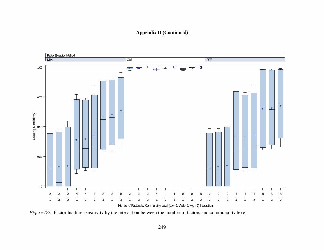
Appendix D (Continued)
249
Figure D2. Factor loading sensitivity by the interaction between the number of factors and communality level
2-1
2-2
2-3
4-1
4-2
4-3
8-1
8-2
8-3
2-1
2-2
2-3
4-1
4-2
4-3
8-1
8-2
8-3
2-1
2-2
2-3
4-1
4-2
4-3
8-1
8-2
8-3
0
0.25
0.50
0.75
1.00
Load
ing
Sen
sitiv
ity
Number of Factors by Communality Level (Low=1, Wide=2, High=3) Interaction
MAX OLS PAF
Factor Extraction Method
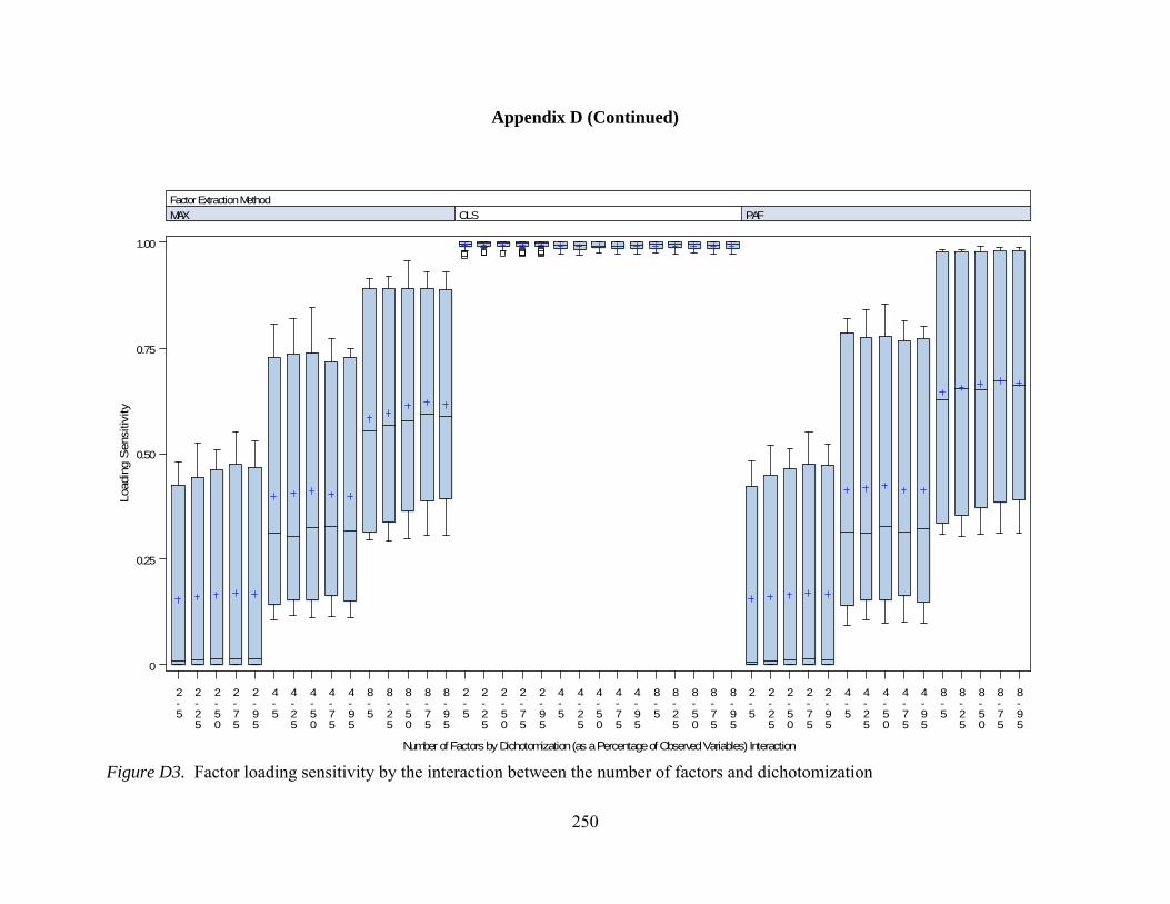
Appendix D (Continued)
250
Figure D3. Factor loading sensitivity by the interaction between the number of factors and dichotomization
2-5
2-25
2-50
2-75
2-95
4-5
4-25
4-50
4-75
4-95
8-5
8-25
8-50
8-75
8-95
2-5
2-25
2-50
2-75
2-95
4-5
4-25
4-50
4-75
4-95
8-5
8-25
8-50
8-75
8-95
2-5
2-25
2-50
2-75
2-95
4-5
4-25
4-50
4-75
4-95
8-5
8-25
8-50
8-75
8-95
0
0.25
0.50
0.75
1.00
Load
ing
Sen
sitiv
ity
Number of Factors by Dichotomization (as a Percentage of Observed Variables) Interaction
MAX OLS PAF
Factor Extraction Method

Appendix D (Continued)
251
Figure D4. Factor loading sensitivity by the interaction between the number of observed variables by communality level
20-1
20-2
20-3
40-1
40-2
40-3
60-1
60-2
60-3
20-1
20-2
20-3
40-1
40-2
40-3
60-1
60-2
60-3
20-1
20-2
20-3
40-1
40-2
40-3
60-1
60-2
60-3
0
0.25
0.50
0.75
1.00
Load
ing
Sen
sitiv
ity
Number of Observed Variables by Communality Level (Low=1, Wide=2, High=3) Interaction
MAX OLS PAF
Factor Extraction Method

Appendix D (Continued)
252
Figure D5. General factor pattern agreement by the interaction between the number of factors and observed variables
2-20
2-40
2-60
4-20
4-40
4-60
8-20
8-40
8-60
2-20
2-40
2-60
4-20
4-40
4-60
8-20
8-40
8-60
2-20
2-40
2-60
4-20
4-40
4-60
8-20
8-40
8-60
0
0.25
0.50
0.75
1.00
Gen
eral
Pat
tern
Agr
eem
ent
Number of Factors by Number of Observed Variables Interaction
MAX OLS PAF
Factor Extraction Method

Appendix D (Continued)
253
Figure D6. General factor pattern agreement by the interaction between the number of factors and communality level
2-1
2-2
2-3
4-1
4-2
4-3
8-1
8-2
8-3
2-1
2-2
2-3
4-1
4-2
4-3
8-1
8-2
8-3
2-1
2-2
2-3
4-1
4-2
4-3
8-1
8-2
8-3
0
0.25
0.50
0.75
1.00
Gen
eral
Pat
tern
Agr
eem
ent
Number of Factors by Communality Level (Low=1, Wide=2, High=3) Interaction
MAX OLS PAF
Factor Extraction Method
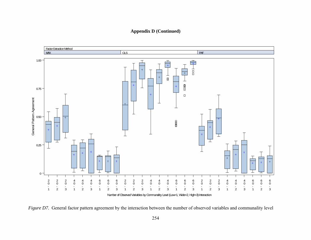
Appendix D (Continued)
254
Figure D7. General factor pattern agreement by the interaction between the number of observed variables and communality level
20-1
20-2
20-3
40-1
40-2
40-3
60-1
60-2
60-3
20-1
20-2
20-3
40-1
40-2
40-3
60-1
60-2
60-3
20-1
20-2
20-3
40-1
40-2
40-3
60-1
60-2
60-3
0
0.25
0.50
0.75
1.00
Gen
eral
Pat
tern
Agr
eem
ent
Number of Observed Variables by Communality Level (Low=1, Wide=2, High=3) Interaction
MAX OLS PAF
Factor Extraction Method
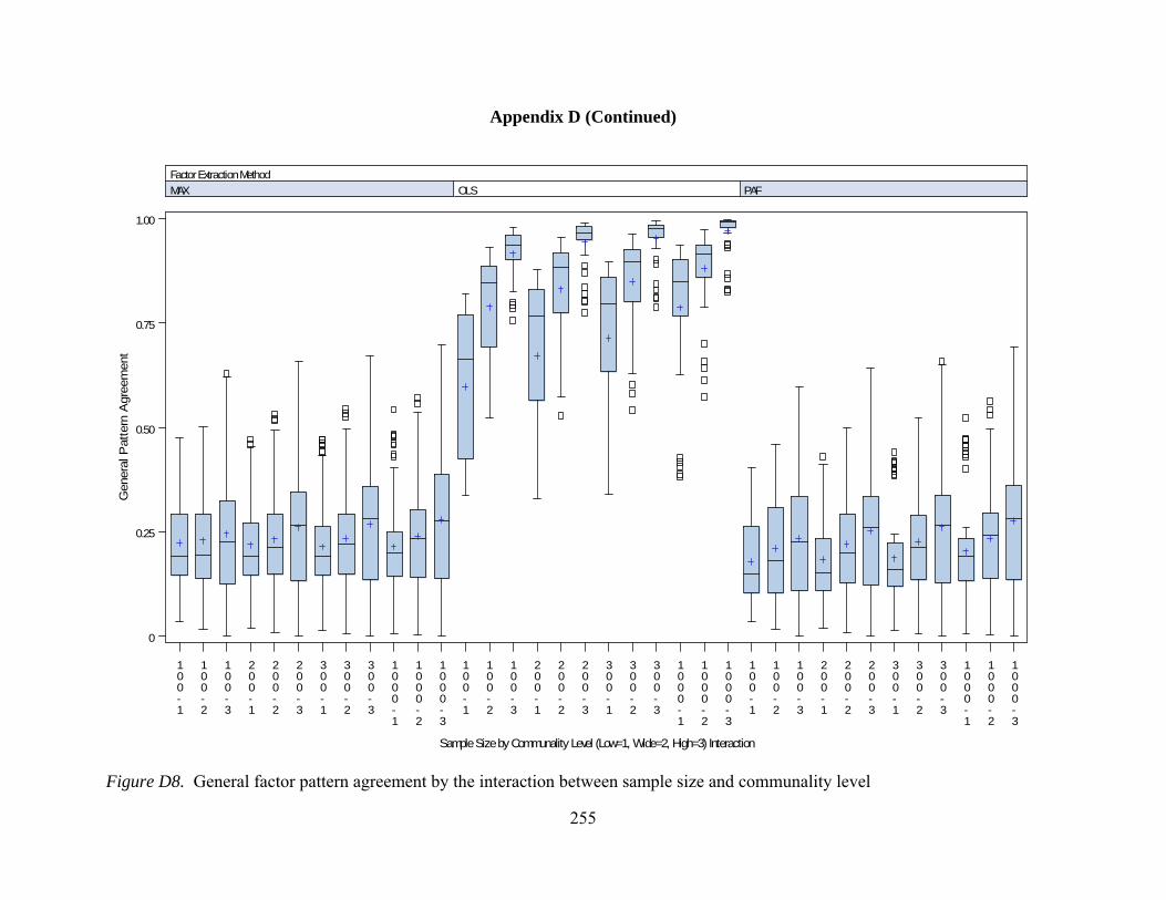
Appendix D (Continued)
255
Figure D8. General factor pattern agreement by the interaction between sample size and communality level
100-1
100-2
100-3
200-1
200-2
200-3
300-1
300-2
300-3
1000-1
1000-2
1000-3
100-1
100-2
100-3
200-1
200-2
200-3
300-1
300-2
300-3
1000-1
1000-2
1000-3
100-1
100-2
100-3
200-1
200-2
200-3
300-1
300-2
300-3
1000-1
1000-2
1000-3
0
0.25
0.50
0.75
1.00
Gen
eral
Pat
tern
Agr
eem
ent
Sample Size by Communality Level (Low=1, Wide=2, High=3) Interaction
MAX OLS PAF
Factor Extraction Method

Appendix D (Continued)
256
Figure D9. Per element factor pattern agreement by the interaction between number of factors and number of observed variables
2-20
2-40
2-60
4-20
4-40
4-60
8-20
8-40
8-60
2-20
2-40
2-60
4-20
4-40
4-60
8-20
8-40
8-60
2-20
2-40
2-60
4-20
4-40
4-60
8-20
8-40
8-60
0
0.2
0.4
0.6
0.8
1.0
Per
Ele
men
t A
gree
men
t
Number of Factors by Number of Observed Variables Interaction
MAX OLS PAF
Factor Extraction Method
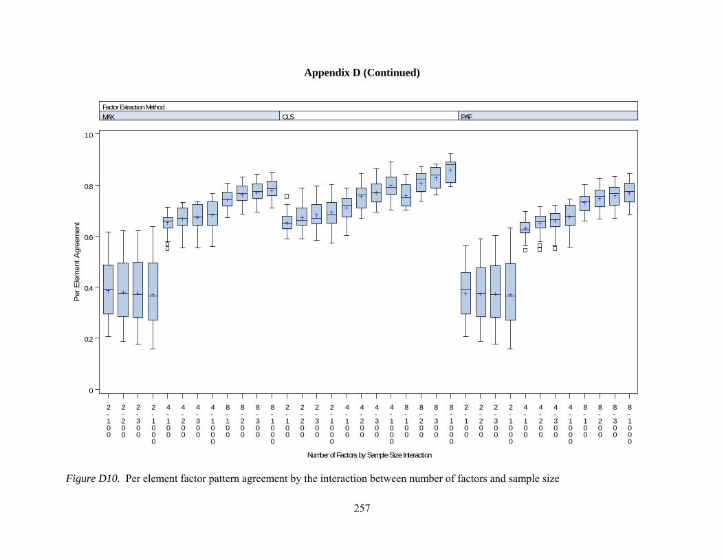
Appendix D (Continued)
257
Figure D10. Per element factor pattern agreement by the interaction between number of factors and sample size
2-100
2-200
2-300
2-1000
4-100
4-200
4-300
4-1000
8-100
8-200
8-300
8-1000
2-100
2-200
2-300
2-1000
4-100
4-200
4-300
4-1000
8-100
8-200
8-300
8-1000
2-100
2-200
2-300
2-1000
4-100
4-200
4-300
4-1000
8-100
8-200
8-300
8-1000
0
0.2
0.4
0.6
0.8
1.0
Per
Ele
men
t A
gree
men
t
Number of Factors by Sample Size Interaction
MAX OLS PAF
Factor Extraction Method
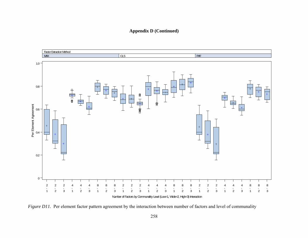
Appendix D (Continued)
258
Figure D11. Per element factor pattern agreement by the interaction between number of factors and level of communality
2-1
2-2
2-3
4-1
4-2
4-3
8-1
8-2
8-3
2-1
2-2
2-3
4-1
4-2
4-3
8-1
8-2
8-3
2-1
2-2
2-3
4-1
4-2
4-3
8-1
8-2
8-3
0
0.2
0.4
0.6
0.8
1.0
Per
Ele
men
t A
gree
men
t
Number of Factors by Communality Level (Low=1, Wide=2, High=3) Interaction
MAX OLS PAF
Factor Extraction Method
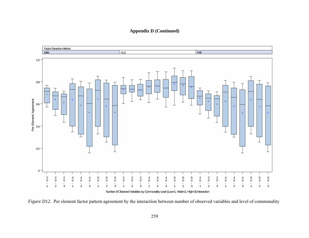
Appendix D (Continued)
259
Figure D12. Per element factor pattern agreement by the interaction between number of observed variables and level of communality
20-1
20-2
20-3
40-1
40-2
40-3
60-1
60-2
60-3
20-1
20-2
20-3
40-1
40-2
40-3
60-1
60-2
60-3
20-1
20-2
20-3
40-1
40-2
40-3
60-1
60-2
60-3
0
0.2
0.4
0.6
0.8
1.0
Per
Ele
men
t A
gree
men
t
Number of Observed Variables by Communality Level (Low=1, Wide=2, High=3) Interaction
MAX OLS PAF
Factor Extraction Method
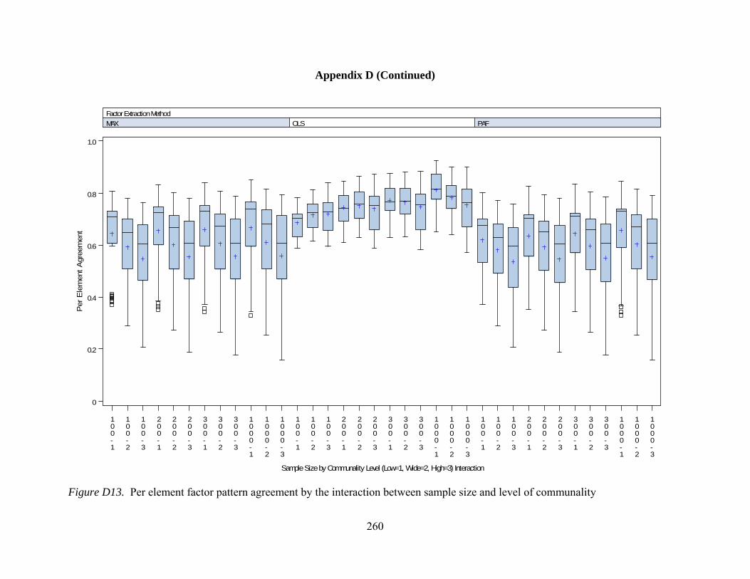
Appendix D (Continued)
260
Figure D13. Per element factor pattern agreement by the interaction between sample size and level of communality
100-1
100-2
100-3
200-1
200-2
200-3
300-1
300-2
300-3
1000-1
1000-2
1000-3
100-1
100-2
100-3
200-1
200-2
200-3
300-1
300-2
300-3
1000-1
1000-2
1000-3
100-1
100-2
100-3
200-1
200-2
200-3
300-1
300-2
300-3
1000-1
1000-2
1000-3
0
0.2
0.4
0.6
0.8
1.0
Per
Ele
men
t A
gree
men
t
Sample Size by Communality Level (Low=1, Wide=2, High=3) Interaction
MAX OLS PAF
Factor Extraction Method

Appendix D (Continued)
261
Figure D14. Total factor pattern agreement by the interaction between the number of factors and number of observed variables
2-20
2-40
2-60
4-20
4-40
4-60
8-20
8-40
8-60
2-20
2-40
2-60
4-20
4-40
4-60
8-20
8-40
8-60
2-20
2-40
2-60
4-20
4-40
4-60
8-20
8-40
8-60
0
0.0025
0.0050
0.0075
0.0100
Tot
al A
gree
men
t
Number of Factors by Number of Observed Variables Interaction
MAX OLS PAF
Factor Extraction Method

Appendix D (Continued)
262
Figure D15. Total factor pattern agreement by the interaction between the number of factors and sample size
2-100
2-200
2-300
2-1000
4-100
4-200
4-300
4-1000
8-100
8-200
8-300
8-1000
2-100
2-200
2-300
2-1000
4-100
4-200
4-300
4-1000
8-100
8-200
8-300
8-1000
2-100
2-200
2-300
2-1000
4-100
4-200
4-300
4-1000
8-100
8-200
8-300
8-1000
0
0.0025
0.0050
0.0075
0.0100
Tot
al A
gree
men
t
Number of Factors by Sample Size Interaction
MAX OLS PAF
Factor Extraction Method
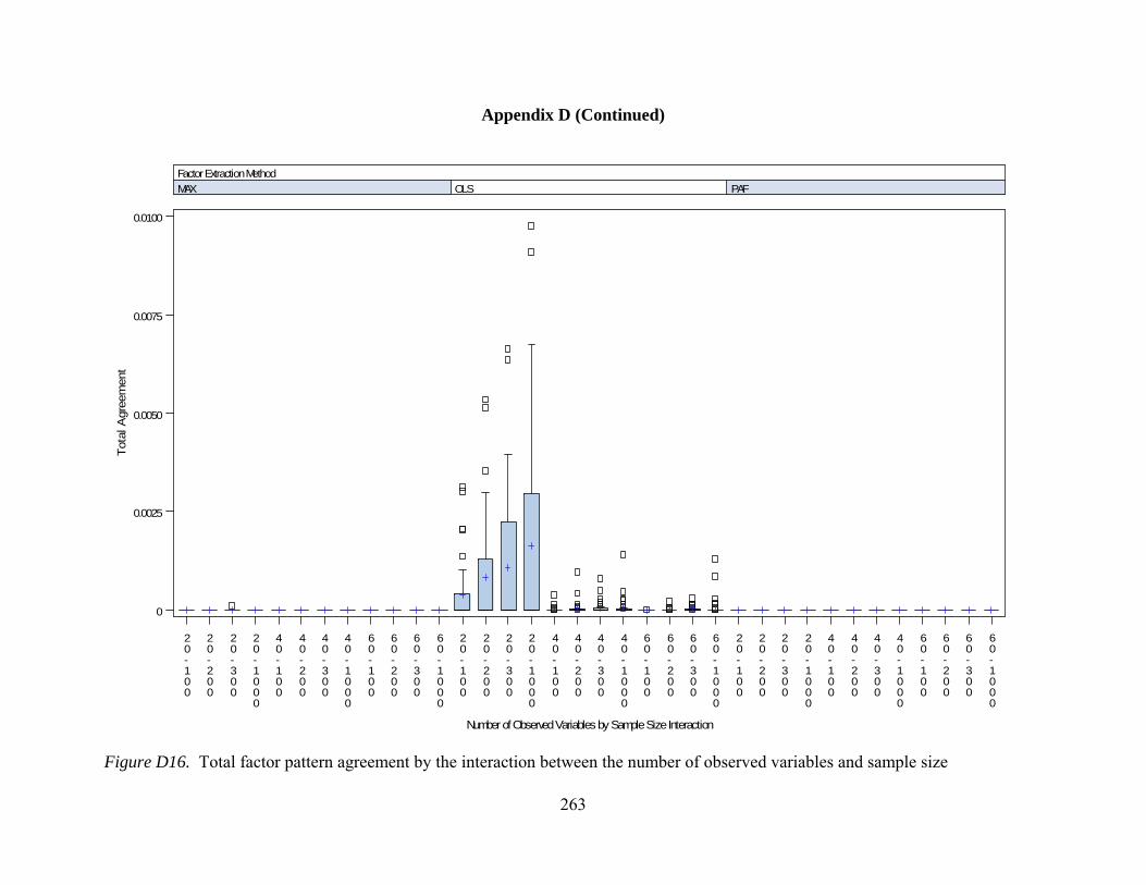
Appendix D (Continued)
263
Figure D16. Total factor pattern agreement by the interaction between the number of observed variables and sample size
20-100
20-200
20-300
20-1000
40-100
40-200
40-300
40-1000
60-100
60-200
60-300
60-1000
20-100
20-200
20-300
20-1000
40-100
40-200
40-300
40-1000
60-100
60-200
60-300
60-1000
20-100
20-200
20-300
20-1000
40-100
40-200
40-300
40-1000
60-100
60-200
60-300
60-1000
0
0.0025
0.0050
0.0075
0.0100
Tot
al A
gree
men
t
Number of Observed Variables by Sample Size Interaction
MAX OLS PAF
Factor Extraction Method

Appendix D (Continued)
264
Figure D17. Mean Phi Values by the interaction between the number of factors and number of observed variables
2-20
2-40
2-60
4-20
4-40
4-60
8-20
8-40
8-60
2-20
2-40
2-60
4-20
4-40
4-60
8-20
8-40
8-60
2-20
2-40
2-60
4-20
4-40
4-60
8-20
8-40
8-60
0
0.2
0.4
0.6
0.8
1.0
Mea
n P
hi V
alue
s
Number of Factors by Number of Observed Variables Interaction
MAX OLS PAF
Factor Extraction Method

Appendix D (Continued)
265
Figure D18. Mean Phi Values by the interaction between the number of factors and sample size
2-100
2-200
2-300
2-1000
4-100
4-200
4-300
4-1000
8-100
8-200
8-300
8-1000
2-100
2-200
2-300
2-1000
4-100
4-200
4-300
4-1000
8-100
8-200
8-300
8-1000
2-100
2-200
2-300
2-1000
4-100
4-200
4-300
4-1000
8-100
8-200
8-300
8-1000
0
0.2
0.4
0.6
0.8
1.0
Mea
n P
hi V
alue
s
Number of Factors by Sample Size Interaction
MAX OLS PAF
Factor Extraction Method

Appendix D (Continued)
266
Figure D19. Mean Phi Values by the interaction between the number of factors and level of dichotomization
2-5
2-25
2-50
2-75
2-95
4-5
4-25
4-50
4-75
4-95
8-5
8-25
8-50
8-75
8-95
2-5
2-25
2-50
2-75
2-95
4-5
4-25
4-50
4-75
4-95
8-5
8-25
8-50
8-75
8-95
2-5
2-25
2-50
2-75
2-95
4-5
4-25
4-50
4-75
4-95
8-5
8-25
8-50
8-75
8-95
0
0.2
0.4
0.6
0.8
1.0
Mea
n P
hi V
alue
s
Number of Factors by Dichotomization (as a Percentage of Observed Variables) Interaction
MAX OLS PAF
Factor Extraction Method
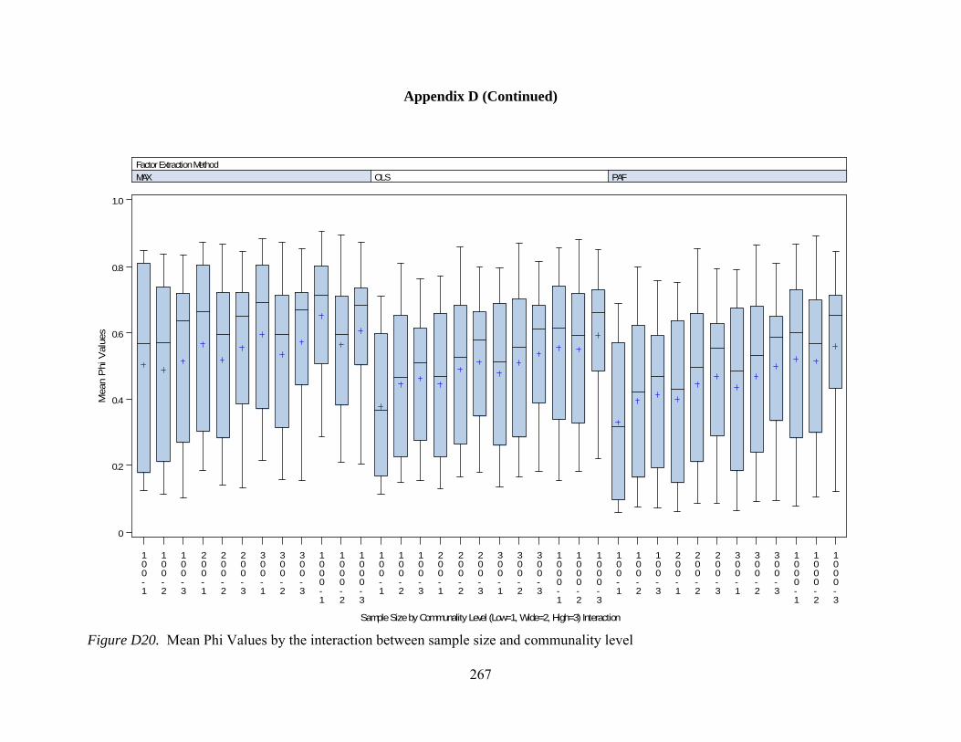
Appendix D (Continued)
267
Figure D20. Mean Phi Values by the interaction between sample size and communality level
100-1
100-2
100-3
200-1
200-2
200-3
300-1
300-2
300-3
1000-1
1000-2
1000-3
100-1
100-2
100-3
200-1
200-2
200-3
300-1
300-2
300-3
1000-1
1000-2
1000-3
100-1
100-2
100-3
200-1
200-2
200-3
300-1
300-2
300-3
1000-1
1000-2
1000-3
0
0.2
0.4
0.6
0.8
1.0
Mea
n P
hi V
alue
s
Sample Size by Communality Level (Low=1, Wide=2, High=3) Interaction
MAX OLS PAF
Factor Extraction Method

Appendix D (Continued)
268
Figure D21. Mean Phi Values by the interaction between levels of communality and dichotomization
1-5
1-25
1-50
1-75
1-95
2-5
2-25
2-50
2-75
2-95
3-5
3-25
3-50
3-75
3-95
1-5
1-25
1-50
1-75
1-95
2-5
2-25
2-50
2-75
2-95
3-5
3-25
3-50
3-75
3-95
1-5
1-25
1-50
1-75
1-95
2-5
2-25
2-50
2-75
2-95
3-5
3-25
3-50
3-75
3-95
0
0.2
0.4
0.6
0.8
1.0
Mea
n P
hi V
alue
s
Communality Level (Low=1, Wide=2, High=3) by Dichotomization (as a Percentage of Observed Variables) Interaction
MAX OLS PAF
Factor Extraction Method
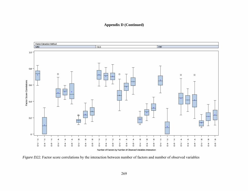
Appendix D (Continued)
269
Figure D22. Factor score correlations by the interaction between number of factors and number of observed variables
2-20
2-40
2-60
4-20
4-40
4-60
8-20
8-40
8-60
2-20
2-40
2-60
4-20
4-40
4-60
8-20
8-40
8-60
2-20
2-40
2-60
4-20
4-40
4-60
8-20
8-40
8-60
0
0.2
0.4
0.6
0.8
1.0
Fac
tor S
core
Cor
rela
tions
Number of Factors by Number of Observed Variables Interaction
MAX OLS PAF
Factor Extraction Method
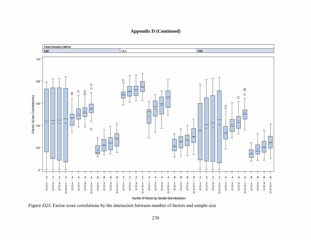
Appendix D (Continued)
270
Figure D23. Factor score correlations by the interaction between number of factors and sample size
2-100
2-200
2-300
2-1000
4-100
4-200
4-300
4-1000
8-100
8-200
8-300
8-1000
2-100
2-200
2-300
2-1000
4-100
4-200
4-300
4-1000
8-100
8-200
8-300
8-1000
2-100
2-200
2-300
2-1000
4-100
4-200
4-300
4-1000
8-100
8-200
8-300
8-1000
0
0.2
0.4
0.6
0.8
1.0
Fac
tor
Sco
re C
orre
latio
nss
Number of Factors by Sample Size Interaction
MAX OLS PAF
Factor Extraction Method

Appendix D (Continued)
271
Figure D24. Factor score correlations by the interaction between number of factors and communality level
2-1
2-2
2-3
4-1
4-2
4-3
8-1
8-2
8-3
2-1
2-2
2-3
4-1
4-2
4-3
8-1
8-2
8-3
2-1
2-2
2-3
4-1
4-2
4-3
8-1
8-2
8-3
0
0.2
0.4
0.6
0.8
1.0
Fac
tor
Sco
re C
orre
latio
ns
Number of Factors by Communality Level (Low=1, Wide=2, High=3) Interaction
MAX OLS PAF
Factor Extraction Method

Appendix D (Continued)
272
Figure D25. Factor loading bias by the interaction between the number of factors and number of observed variables
2-20
2-40
2-60
4-20
4-40
4-60
8-20
8-40
8-60
2-20
2-40
2-60
4-20
4-40
4-60
8-20
8-40
8-60
2-20
2-40
2-60
4-20
4-40
4-60
8-20
8-40
8-60
-0.3
-0.2
-0.1
0
0.1
Fac
tor
Load
ing
Bia
s
Number of Factors by Number of Observed Variables Interaction
MAX OLS PAF
Factor Extraction Method
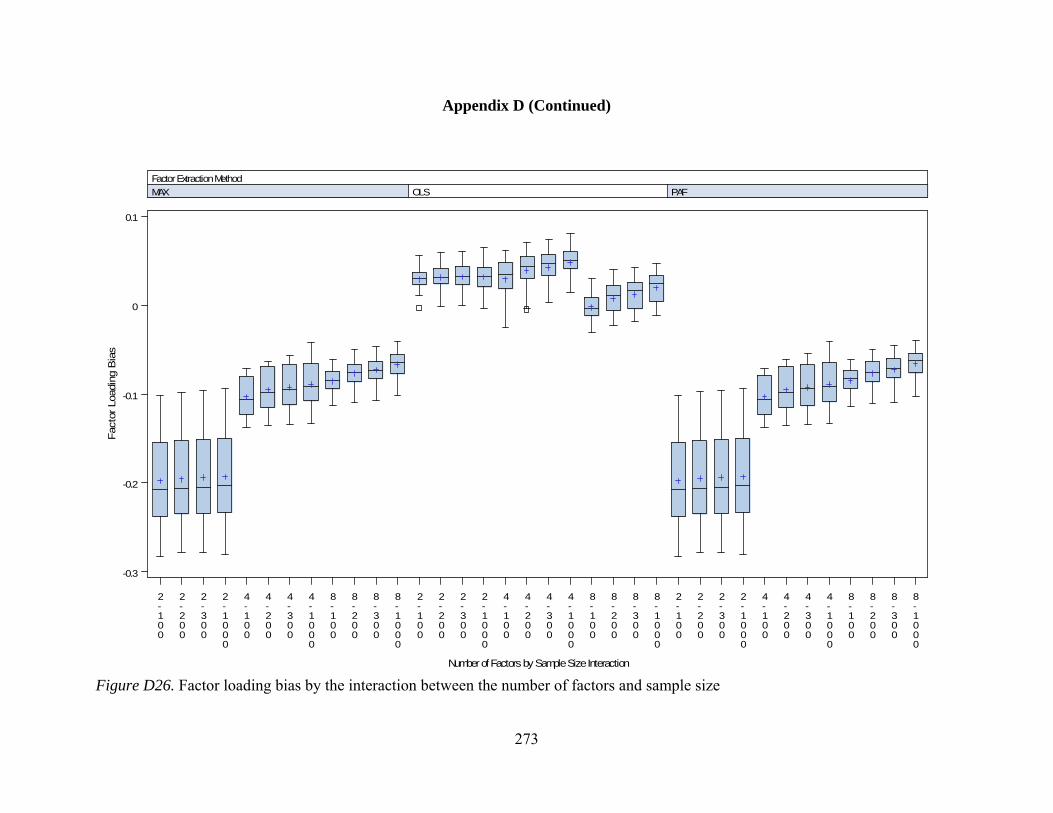
Appendix D (Continued)
273
Figure D26. Factor loading bias by the interaction between the number of factors and sample size
2-100
2-200
2-300
2-1000
4-100
4-200
4-300
4-1000
8-100
8-200
8-300
8-1000
2-100
2-200
2-300
2-1000
4-100
4-200
4-300
4-1000
8-100
8-200
8-300
8-1000
2-100
2-200
2-300
2-1000
4-100
4-200
4-300
4-1000
8-100
8-200
8-300
8-1000
-0.3
-0.2
-0.1
0
0.1
Fac
tor Lo
adin
g B
ias
Number of Factors by Sample Size Interaction
MAX OLS PAF
Factor Extraction Method

Appendix D (Continued)
274
Figure D27. Factor loading bias by the interaction between the number of factors and communality
2-1
2-2
2-3
4-1
4-2
4-3
8-1
8-2
8-3
2-1
2-2
2-3
4-1
4-2
4-3
8-1
8-2
8-3
2-1
2-2
2-3
4-1
4-2
4-3
8-1
8-2
8-3
-0.3
-0.2
-0.1
0
0.1
Fac
tor Lo
adin
g B
ias
Number of Factors by Communality Level (Low=1, Wide=2, High=3) Interaction
MAX OLS PAF
Factor Extraction Method

Appendix D (Continued)
275
Figure D28. Factor loading bias by the interaction between the number of factors and level of dichotomization
2-5
2-25
2-50
2-75
2-95
4-5
4-25
4-50
4-75
4-95
8-5
8-25
8-50
8-75
8-95
2-5
2-25
2-50
2-75
2-95
4-5
4-25
4-50
4-75
4-95
8-5
8-25
8-50
8-75
8-95
2-5
2-25
2-50
2-75
2-95
4-5
4-25
4-50
4-75
4-95
8-5
8-25
8-50
8-75
8-95
-0.3
-0.2
-0.1
0
0.1
Fac
tor
Load
ing
Bia
s
Number of Factors by Dichotomization (as a Percentage of Observed Variables) Interaction
MAX OLS PAF
Factor Extraction Method
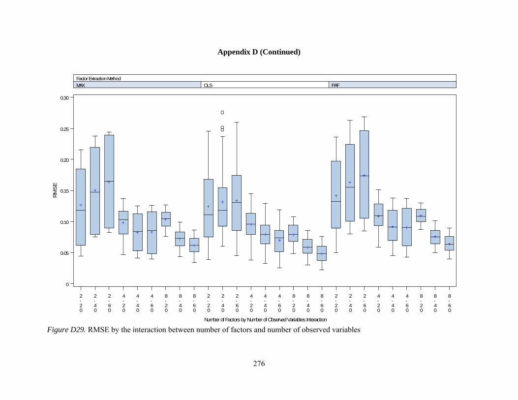
Appendix D (Continued)
276
Figure D29. RMSE by the interaction between number of factors and number of observed variables
2-20
2-40
2-60
4-20
4-40
4-60
8-20
8-40
8-60
2-20
2-40
2-60
4-20
4-40
4-60
8-20
8-40
8-60
2-20
2-40
2-60
4-20
4-40
4-60
8-20
8-40
8-60
0
0.05
0.10
0.15
0.20
0.25
0.30
RM
SE
Number of Factors by Number of Observed Variables Interaction
MAX OLS PAF
Factor Extraction Method
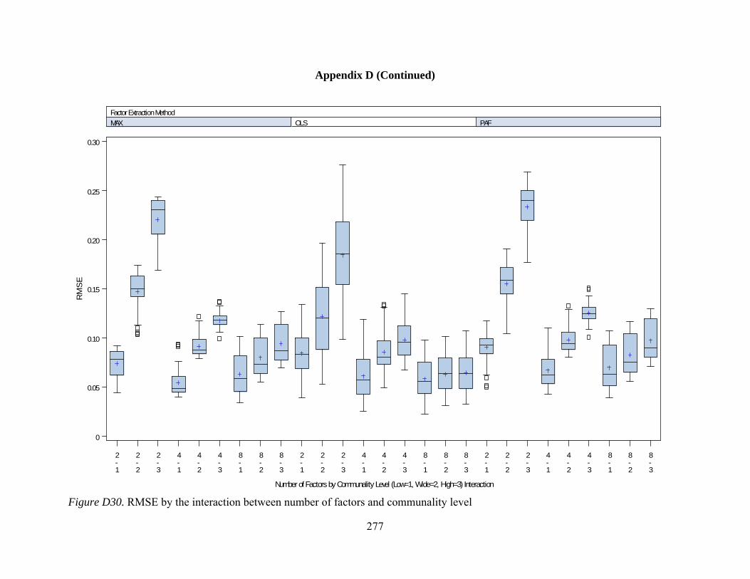
Appendix D (Continued)
277
Figure D30. RMSE by the interaction between number of factors and communality level
2-1
2-2
2-3
4-1
4-2
4-3
8-1
8-2
8-3
2-1
2-2
2-3
4-1
4-2
4-3
8-1
8-2
8-3
2-1
2-2
2-3
4-1
4-2
4-3
8-1
8-2
8-3
0
0.05
0.10
0.15
0.20
0.25
0.30
RM
SE
Number of Factors by Communality Level (Low=1, Wide=2, High=3) Interaction
MAX OLS PAF
Factor Extraction Method

Appendix D (Continued)
278
Figure D31. RMSE by the interaction between number of factors and level of dichotomization
2-5
2-25
2-50
2-75
2-95
4-5
4-25
4-50
4-75
4-95
8-5
8-25
8-50
8-75
8-95
2-5
2-25
2-50
2-75
2-95
4-5
4-25
4-50
4-75
4-95
8-5
8-25
8-50
8-75
8-95
2-5
2-25
2-50
2-75
2-95
4-5
4-25
4-50
4-75
4-95
8-5
8-25
8-50
8-75
8-95
0
0.05
0.10
0.15
0.20
0.25
0.30
RM
SE
Number of Factors by Dichotomization (as a Percentage of Observed Variables)Interaction
MAX OLS PAF
Factor Extraction Method

Appendix D (Continued)
279
Figure D32. RMSE by the interaction between level of communality and dichotomization
1-5
1-25
1-50
1-75
1-95
2-5
2-25
2-50
2-75
2-95
3-5
3-25
3-50
3-75
3-95
1-5
1-25
1-50
1-75
1-95
2-5
2-25
2-50
2-75
2-95
3-5
3-25
3-50
3-75
3-95
1-5
1-25
1-50
1-75
1-95
2-5
2-25
2-50
2-75
2-95
3-5
3-25
3-50
3-75
3-95
0
0.05
0.10
0.15
0.20
0.25
0.30
RM
SE
Communality Level (Low=1, Wide=2, High=3) by Dichotomization (as a Percentage of Observed Variables) Interaction
MAX OLS PAF
Factor Extraction Method

Appendix E
280
Simulation Program: SAS, IML© option ls = 256 ps = max nonumber nodate nocenter; proc printto print='c:\EFA_full.lst'; proc iml; **********************************************************************; *************** Begin Specification of Data Conditions ***************; **********************************************************************; p = 60; *20; *40; *60; k = 2; *2; *4; *8; d_frac = .50; *.05; *.25; *.50; *.75; *.95; Commun_type = 1; * commun_type =1, low communalities, elements = .2, .3 or .4; * commun_type =2, wide communalities, elements = .2, .3, .4 ,.5, .6, .7 or .8; * commun_type =3, high communalities, elements = .6, .7 or .8; N_pops = 10; * N of populations to generate; replicat=1000; * N of samples from each population; *replicat=10; * N of samples from each population for testing; /*Inputs for Gendata2 A and B modules*/ nn1 = 100000; means=j(1,p,0); variance = j(1,p,1); ********************************************************************; *************** End Specification of Data Conditions ***************; *************** Begin Subroutines for the Program ******************; ********************************************************************; start Make_PopR(nvars,nfactors,commun_type,A1,R); * program to generate the population covariance matrices based on Tucker, Koopman, & Linn, 1969, Psychometrica; * Inputs are nvars = number of variables in the matrix nfactors = number of factors commun = Type of communality Output is R = population correlation matrix; * construct B1square such that commun=1, low communalities, elements = .2, .3 or .4
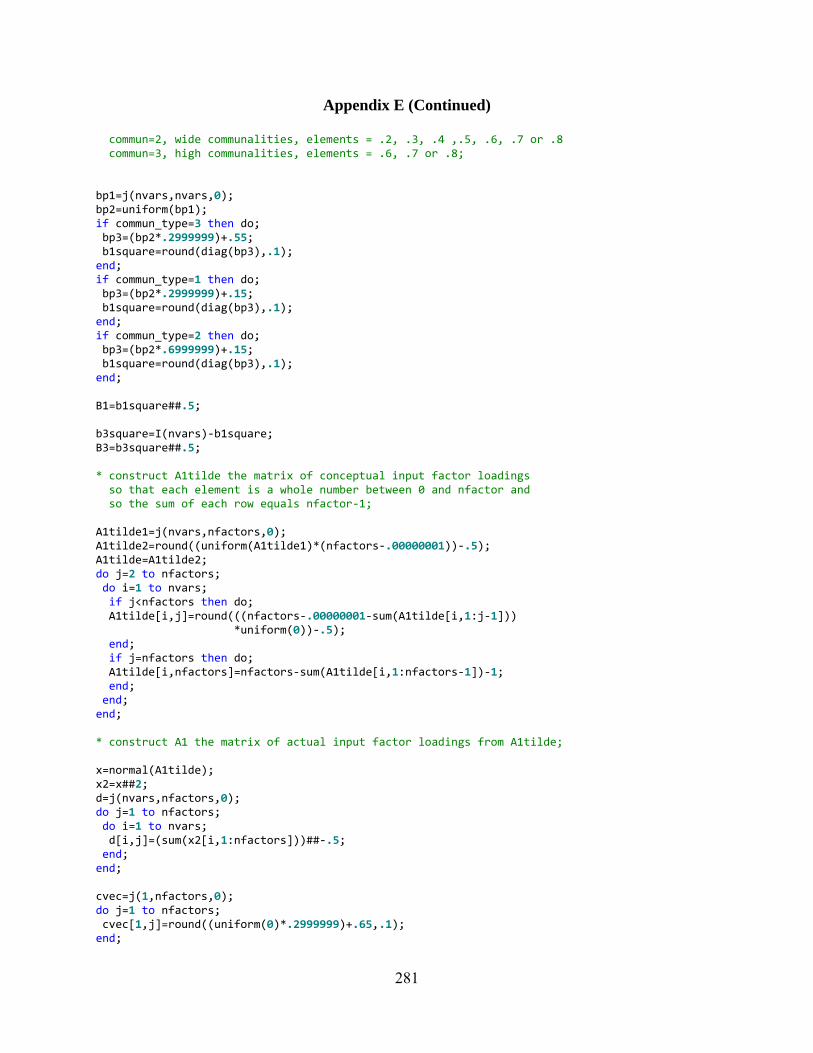
Appendix E (Continued)
281
commun=2, wide communalities, elements = .2, .3, .4 ,.5, .6, .7 or .8 commun=3, high communalities, elements = .6, .7 or .8; bp1=j(nvars,nvars,0); bp2=uniform(bp1); if commun_type=3 then do; bp3=(bp2*.2999999)+.55; b1square=round(diag(bp3),.1); end; if commun_type=1 then do; bp3=(bp2*.2999999)+.15; b1square=round(diag(bp3),.1); end; if commun_type=2 then do; bp3=(bp2*.6999999)+.15; b1square=round(diag(bp3),.1); end; B1=b1square##.5; b3square=I(nvars)‐b1square; B3=b3square##.5; * construct A1tilde the matrix of conceptual input factor loadings so that each element is a whole number between 0 and nfactor and so the sum of each row equals nfactor‐1; A1tilde1=j(nvars,nfactors,0); A1tilde2=round((uniform(A1tilde1)*(nfactors‐.00000001))‐.5); A1tilde=A1tilde2; do j=2 to nfactors; do i=1 to nvars; if j<nfactors then do; A1tilde[i,j]=round(((nfactors‐.00000001‐sum(A1tilde[i,1:j‐1])) *uniform(0))‐.5); end; if j=nfactors then do; A1tilde[i,nfactors]=nfactors‐sum(A1tilde[i,1:nfactors‐1])‐1; end; end; end; * construct A1 the matrix of actual input factor loadings from A1tilde; x=normal(A1tilde); x2=x##2; d=j(nvars,nfactors,0); do j=1 to nfactors; do i=1 to nvars; d[i,j]=(sum(x2[i,1:nfactors]))##‐.5; end; end; cvec=j(1,nfactors,0); do j=1 to nfactors; cvec[1,j]=round((uniform(0)*.2999999)+.65,.1); end;

Appendix E (Continued)
282
c=j(nvars,1,1)*cvec; c2=c##2; ones=j(nvars,nfactors,1); y=A1tilde#c + d#x#((ones‐c2)##.5); k=.2; z=j(nvars,nfactors,0); do j=1 to nfactors; do i=1 to nvars; z[i,j]=((1+k)*y[i,j]*(y[i,j]+abs(y[i,j])+k))/((2+k)*(abs(y[i,j])+k)); end; end; z2=z##2; g=j(nvars,nfactors,0); do j=1 to nfactors; do i=1 to nvars; g[i,j]=(sum(z2[i,1:nfactors]))##‐.5; end; end; A1star=g#z; A1=B1*A1star; A3star=I(nvars); A3=B3*A3star; R=A1*A1`+A3*A3`; Finish; start gendata2a(NN1,seed1,variance,bb,cc,dd,mu,r_matrix,YY,p,d_frac); L = eigval(r_matrix); neg_eigval = 0; do r = 1 to nrow(L); if L[r,1] < 0 then neg_eigval = 1; end; if neg_eigval = 0 then do; * matrix is positive definite, so use the Cholesky root approach; COLS = NCOL(r_matrix); G = ROOT(r_matrix); YY=rannor(repeat(seed1,nn1,COLS)); YY = YY*G; do r = 1 to NN1; do c = 1 to COLS; YY[r,c] = (‐1*cc) + (bb*YY[r,c]) + (cc*YY[r,c]##2) + (dd*YY[r,c]##3); YY[r,c] = (YY[r,c] * SQRT(variance[1,c])) + mu[1,c]; end; end; end; if neg_eigval = 1 then do; * matrix is not positive definite, so use the PCA approach; COLS = NCOL(r_matrix); V = eigvec(r_matrix); do i = 1 to nrow(L); do j = 1 to ncol(V);
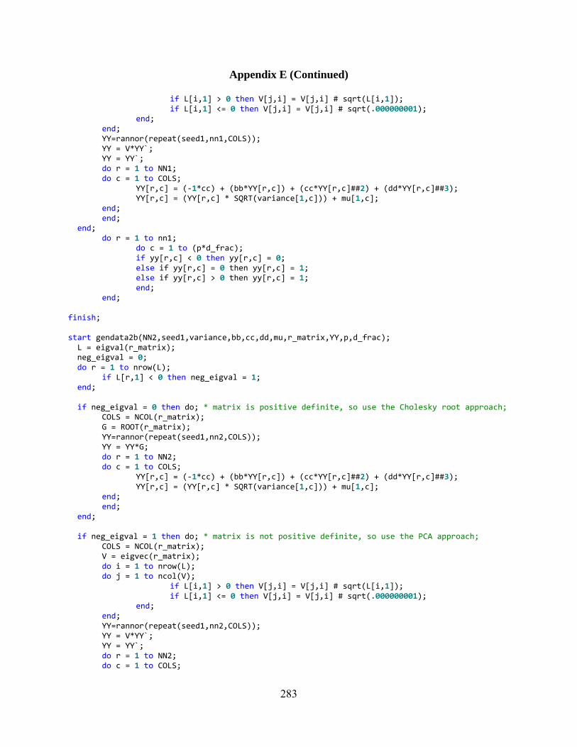
Appendix E (Continued)
283
if L[i,1] > 0 then V[j,i] = V[j,i] # sqrt(L[i,1]); if L[i,1] <= 0 then V[j,i] = V[j,i] # sqrt(.000000001); end; end; YY=rannor(repeat(seed1,nn1,COLS)); YY = V*YY`; YY = YY`; do r = 1 to NN1; do c = 1 to COLS; YY[r,c] = (‐1*cc) + (bb*YY[r,c]) + (cc*YY[r,c]##2) + (dd*YY[r,c]##3); YY[r,c] = (YY[r,c] * SQRT(variance[1,c])) + mu[1,c]; end; end; end; do r = 1 to nn1; do c = 1 to (p*d_frac); if yy[r,c] < 0 then yy[r,c] = 0; else if yy[r,c] = 0 then yy[r,c] = 1; else if yy[r,c] > 0 then yy[r,c] = 1; end; end; finish; start gendata2b(NN2,seed1,variance,bb,cc,dd,mu,r_matrix,YY,p,d_frac); L = eigval(r_matrix); neg_eigval = 0; do r = 1 to nrow(L); if L[r,1] < 0 then neg_eigval = 1; end; if neg_eigval = 0 then do; * matrix is positive definite, so use the Cholesky root approach; COLS = NCOL(r_matrix); G = ROOT(r_matrix); YY=rannor(repeat(seed1,nn2,COLS)); YY = YY*G; do r = 1 to NN2; do c = 1 to COLS; YY[r,c] = (‐1*cc) + (bb*YY[r,c]) + (cc*YY[r,c]##2) + (dd*YY[r,c]##3); YY[r,c] = (YY[r,c] * SQRT(variance[1,c])) + mu[1,c]; end; end; end; if neg_eigval = 1 then do; * matrix is not positive definite, so use the PCA approach; COLS = NCOL(r_matrix); V = eigvec(r_matrix); do i = 1 to nrow(L); do j = 1 to ncol(V); if L[i,1] > 0 then V[j,i] = V[j,i] # sqrt(L[i,1]); if L[i,1] <= 0 then V[j,i] = V[j,i] # sqrt(.000000001); end; end; YY=rannor(repeat(seed1,nn2,COLS)); YY = V*YY`; YY = YY`; do r = 1 to NN2; do c = 1 to COLS;
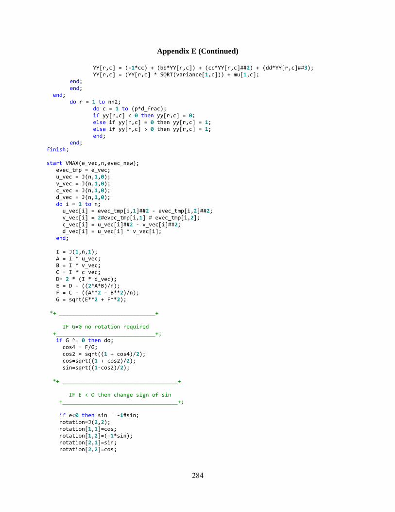
Appendix E (Continued)
284
YY[r,c] = (‐1*cc) + (bb*YY[r,c]) + (cc*YY[r,c]##2) + (dd*YY[r,c]##3); YY[r,c] = (YY[r,c] * SQRT(variance[1,c])) + mu[1,c]; end; end; end; do r = 1 to nn2; do c = 1 to (p*d_frac); if yy[r,c] < 0 then yy[r,c] = 0; else if yy[r,c] = 0 then yy[r,c] = 1; else if yy[r,c] > 0 then yy[r,c] = 1; end; end; finish; start VMAX(e_vec,n,evec_new); evec_tmp = e_vec; u_vec = J(n,1,0); v_vec = J(n,1,0); c_vec = J(n,1,0); d_vec = J(n,1,0); do i = 1 to n; u_vec[i] = evec_tmp[i,1]##2 ‐ evec_tmp[i,2]##2; v_vec[i] = 2#evec_tmp[i,1] # evec_tmp[i,2]; c_vec[i] = u_vec[i]##2 ‐ v_vec[i]##2; d_vec[i] = u_vec[i] * v_vec[i]; end; I = J(1,n,1); A = I * u_vec; B = I * v_vec; C = I * c_vec; D= 2 * (I * d_vec); E = D ‐ ((2*A*B)/n); F = C ‐ ((A**2 ‐ B**2)/n); G = sqrt(E**2 + F**2); *+ ______________________________+ IF G=0 no rotation required +_______________________________+; if G ^= 0 then do; cos4 = F/G; cos2 = sqrt((1 + cos4)/2); cos=sqrt((1 + cos2)/2); sin=sqrt((1‐cos2)/2); *+ ____________________________________+ IF E < O then change sign of sin +____________________________________+; if e<0 then sin = ‐1#sin; rotation=J(2,2); rotation[1,1]=cos; rotation[1,2]=(‐1*sin); rotation[2,1]=sin; rotation[2,2]=cos;
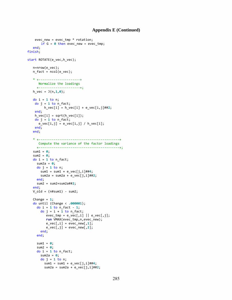
Appendix E (Continued)
285
evec_new = evec_tmp * rotation; if G = 0 then evec_new = evec_tmp; end; finish; start ROTATE(e_vec,h_vec); n=nrow(e_vec); n_fact = ncol(e_vec); * +‐‐‐‐‐‐‐‐‐‐‐‐‐‐‐‐‐‐‐‐‐‐+ Normalize the loadings +‐‐‐‐‐‐‐‐‐‐‐‐‐‐‐‐‐‐‐‐‐‐+; h_vec = J(n,1,0); do i = 1 to n; do j = 1 to n_fact; h_vec[i] = h_vec[i] + e_vec[i,j]##2; end; h_vec[i] = sqrt(h_vec[i]); do j = 1 to n_fact; e_vec[i,j] = e_vec[i,j] / h_vec[i]; end; end; * +‐‐‐‐‐‐‐‐‐‐‐‐‐‐‐‐‐‐‐‐‐‐‐‐‐‐‐‐‐‐‐‐‐‐‐‐‐‐‐‐‐‐‐+ Compute the variance of the factor loadings +‐‐‐‐‐‐‐‐‐‐‐‐‐‐‐‐‐‐‐‐‐‐‐‐‐‐‐‐‐‐‐‐‐‐‐‐‐‐‐‐‐‐‐+; sum1 = 0; sum2 = 0; do i = 1 to n_fact; sum2a = 0; do j = 1 to n; sum1 = sum1 + e_vec[j,i]##4; sum2a = sum2a + e_vec[j,i]##2; end; sum2 = sum2+sum2a##2; end; V_old = (n#sum1) ‐ sum2; Change = 1; do until (Change < .000001); do i = 1 to n_fact ‐ 1; do j = i + 1 to n_fact; evec_tmp = e_vec[,i] || e_vec[,j]; run VMAX(evec_tmp,n,evec_new); e_vec[,i] = evec_new[,1]; e_vec[,j] = evec_new[,2]; end; end; sum1 = 0; sum2 = 0; do i = 1 to n_fact; sum2a = 0; do j = 1 to n; sum1 = sum1 + e_vec[j,i]##4; sum2a = sum2a + e_vec[j,i]##2;

Appendix E (Continued)
286
end; sum2 = sum2+sum2a##2; end; V = (n#sum1) ‐ sum2; Change = ABS(V_old ‐ V); * print V_old V Change; V_old = V; end; do i = 1 to n; do j = 1 to n_fact; e_vec[i,j] = e_vec[i,j] # h_vec[i]; end; end; * +‐‐‐‐‐‐‐‐‐‐‐‐‐‐‐‐‐‐‐‐‐‐‐‐‐‐‐+ Compute final communalities +‐‐‐‐‐‐‐‐‐‐‐‐‐‐‐‐‐‐‐‐‐‐‐‐‐‐‐+; h_vec = J(n,1,0); do i = 1 to n; do j = 1 to n_fact; h_vec[i] = h_vec[i] + e_vec[i,j]##2; end; end; finish; * +‐‐‐‐‐‐‐‐‐‐‐‐‐‐‐‐‐‐‐‐‐‐‐‐‐‐‐‐‐‐‐‐‐‐‐‐‐‐‐‐‐‐‐‐‐‐‐‐‐‐‐‐‐‐‐‐‐‐‐‐‐‐‐‐+ Subroutine computes bias, MSE and accuracy of factor loadings Inputs: L = matrix of sample pattern coefficients Lambda = matrix of population pattern coefficients * +‐‐‐‐‐‐‐‐‐‐‐‐‐‐‐‐‐‐‐‐‐‐‐‐‐‐‐‐‐‐‐‐‐‐‐‐‐‐‐‐‐‐‐‐‐‐‐‐‐‐‐‐‐‐‐‐‐‐‐‐‐‐‐‐‐+; START ACCURACY(L,Lambda,OK_Load,OK_NoLoad,bias_loadings,MSE_loadings, pattern_accuracy,perfect_accuracy, pattern_accuracy30,perfect_accuracy30); p = nrow(L); k = ncol(L); * +‐‐‐‐‐‐‐‐‐‐‐‐‐‐‐‐‐‐‐‐‐‐‐‐‐‐‐‐‐‐‐‐‐‐‐‐‐‐‐‐‐‐‐‐‐+ Determine if each variable loads on at least one factor using the simple .30 rule of thumb * +‐‐‐‐‐‐‐‐‐‐‐‐‐‐‐‐‐‐‐‐‐‐‐‐‐‐‐‐‐‐‐‐‐‐‐‐‐‐‐‐‐‐‐‐‐+; pop_loaded = J(p,1,0); do variable = 1 to p; do factor = 1 to k; if abs(Lambda[variable,factor]) >= .30 then pop_loaded[variable,1] = 1; end; end; * +‐‐‐‐‐‐‐‐‐‐‐‐‐‐‐‐‐‐‐‐‐‐‐‐‐‐‐‐‐‐‐‐‐‐‐‐‐‐‐‐‐‐‐‐‐+ Determine if each variable loads on at least one factor using the simple .30 rule of thumb * +‐‐‐‐‐‐‐‐‐‐‐‐‐‐‐‐‐‐‐‐‐‐‐‐‐‐‐‐‐‐‐‐‐‐‐‐‐‐‐‐‐‐‐‐‐+; sample_loaded = J(p,1,0); do variable = 1 to p;

Appendix E (Continued)
287
do factor = 1 to k; if abs(L[variable,factor]) >= .30 then sample_loaded[variable,1] = 1; end; end; * +‐‐‐‐‐‐‐‐‐‐‐‐‐‐‐‐‐‐‐‐‐‐‐‐‐‐‐‐‐‐‐‐‐‐‐‐‐‐‐‐‐‐‐‐‐‐‐+ Count number of variables that load "somewhere" in both population and sample, and number that do not load "anywhere" in population and sample * +‐‐‐‐‐‐‐‐‐‐‐‐‐‐‐‐‐‐‐‐‐‐‐‐‐‐‐‐‐‐‐‐‐‐‐‐‐‐‐‐‐‐‐‐‐‐‐+; OK_Load = 0; OK_NoLoad = 0; do variable = 1 to p; if sample_loaded[variable,1] = 1 & pop_loaded[variable,1] = 1 then OK_Load = OK_Load + 1; if sample_loaded[variable,1] = 0 & pop_loaded[variable,1] = 0 then OK_NoLoad = OK_NoLoad + 1; end; OK_Load = OK_Load / sum(pop_loaded); * proportion of variables with loading agreement; * +‐‐‐‐‐‐‐‐‐‐‐‐‐‐‐‐‐‐‐‐‐‐‐‐‐‐‐‐‐‐‐‐‐‐‐‐‐‐‐‐‐‐‐‐‐‐‐+ Only compute OK_NoLoad if some variables do not load in the population * +‐‐‐‐‐‐‐‐‐‐‐‐‐‐‐‐‐‐‐‐‐‐‐‐‐‐‐‐‐‐‐‐‐‐‐‐‐‐‐‐‐‐‐‐‐‐‐+; * +‐‐‐‐‐‐‐‐‐‐‐‐‐‐‐‐‐‐‐‐‐‐‐‐‐‐‐‐‐‐‐‐‐‐‐‐‐‐‐‐‐‐‐‐‐‐‐‐‐‐‐‐‐‐‐‐‐‐‐‐‐‐+ 25 Sept: Jeff changed these two statements, using p instead of k * +‐‐‐‐‐‐‐‐‐‐‐‐‐‐‐‐‐‐‐‐‐‐‐‐‐‐‐‐‐‐‐‐‐‐‐‐‐‐‐‐‐‐‐‐‐‐‐‐‐‐‐‐‐‐‐‐‐‐‐‐‐‐+; if sum(pop_loaded) = p then OK_NoLoad = .; if sum(pop_loaded) < p then OK_NoLoad = OK_NoLoad/(p‐sum(pop_loaded)); * +‐‐‐‐‐‐‐‐‐‐‐‐‐‐‐‐‐‐‐‐‐‐‐‐‐‐‐‐‐‐‐‐‐‐‐‐‐‐‐‐‐‐‐‐‐‐‐‐+ Compute bias and MS Error in the factor loadings * +‐‐‐‐‐‐‐‐‐‐‐‐‐‐‐‐‐‐‐‐‐‐‐‐‐‐‐‐‐‐‐‐‐‐‐‐‐‐‐‐‐‐‐‐‐‐‐‐+; bias_loadings=j(p,k,0); MSE_loadings=j(p,k,0); do row =1 to p; bias_loadings[row,]=L[row,]‐lambda[row,]; MSE_loadings[row,]=(L[row,]‐lambda[row,])##2; end; * +‐‐‐‐‐‐‐‐‐‐‐‐‐‐‐‐‐‐‐‐‐‐‐‐‐‐‐‐‐‐‐‐‐‐‐‐‐‐‐‐‐‐‐‐+ Compute pattern accuracy using the .30 thumb * +‐‐‐‐‐‐‐‐‐‐‐‐‐‐‐‐‐‐‐‐‐‐‐‐‐‐‐‐‐‐‐‐‐‐‐‐‐‐‐‐‐‐‐‐+; pattern_accuracy = j(p,k,0); perfect_accuracy = 0; pattern_accuracy30 = j(p,1,0); perfect_accuracy30 = 0; * +‐‐‐‐‐‐‐‐‐‐‐‐‐‐‐‐‐‐‐‐‐‐‐‐‐‐‐‐‐‐‐‐‐‐‐‐‐‐‐‐‐‐‐‐‐‐‐‐‐‐‐‐‐‐‐‐‐‐‐‐‐‐+ 25 Sept: Jeff changed this loop to include the counter NoLoad If a variable does not load (abs>.30) on any factor in both population and sample, 'credit' is given for pattern accuracy * +‐‐‐‐‐‐‐‐‐‐‐‐‐‐‐‐‐‐‐‐‐‐‐‐‐‐‐‐‐‐‐‐‐‐‐‐‐‐‐‐‐‐‐‐‐‐‐‐‐‐‐‐‐‐‐‐‐‐‐‐‐‐+; do variable = 1 to p; NoLoad = 0;

Appendix E (Continued)
288
do factor = 1 to k; if (abs(Lambda[variable,factor]) >= .30 & abs(L[variable,factor]) >= .30) then do; pattern_accuracy[variable,factor] = 1; pattern_accuracy30[variable,1] = 1; end; if (abs(Lambda[variable,factor]) < .30 & abs(L[variable,factor]) < .30) then do; pattern_accuracy[variable,factor] = 1; NoLoad = NoLoad + 1; end; end; if NoLoad = k then pattern_accuracy30[variable,1] = 1; end; if mean(pattern_accuracy) = 1 then perfect_accuracy = 1; if mean(pattern_accuracy30) = 1 then perfect_accuracy30 = 1; finish; *+_________________________________________________________________+ Subroutine to calculate coefficient of congruence ‐ mean phi Inputs: pop = population factor loadings samp = sample factor loadings Output: Meanphi +_________________________________________________________________+; start get_phi(pop,samp,meanphi); k = ncol(pop); num = vecdiag(pop`*samp); den1 = vecdiag(pop`*pop); den2 = vecdiag(samp`*samp); phi_k = J(k,1,0); meanphi = 0; n_terms = 0; do m = 1 to k; if (den1[m,1]>0 & den2[m,1]>0) then do; phi_k[m,1] = num[m,1] / sqrt(den1[m,1]#den2[m,1]); meanphi = meanphi + phi_k[m,1]; n_terms = n_terms + 1; end; if (den1[m,1] = 0 | den2[m,1] = 0) then do; phi_k[m,1] = 999; end; end; meanphi = meanphi / n_terms; finish; start factor_scores(Lambda,L,sampdat,R_fscores,Non_zero); *+________________________________________________________________________+ Compute Factor Score Estimates Create a matrix of scoring coefficients for the sample (SC) [p X k]
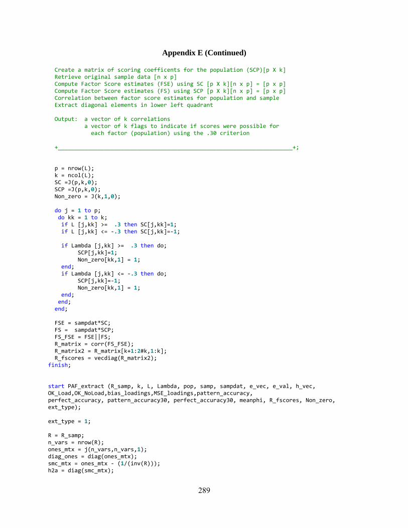
Appendix E (Continued)
289
Create a matrix of scoring coefficents for the population (SCP)[p X k] Retrieve original sample data [n x p] Compute Factor Score estimates (FSE) using SC [p X k][n x p] = [p x p] Compute Factor Score estimates (FS) using SCP [p X k][n x p] = [p x p] Correlation between factor score estimates for population and sample Extract diagonal elements in lower left quadrant Output: a vector of k correlations a vector of k flags to indicate if scores were possible for each factor (population) using the .30 criterion +_______________________________________________________________________+; p = nrow(L); k = ncol(L); SC =J(p,k,0); SCP =J(p,k,0); Non_zero = J(k,1,0); do j = 1 to p; do kk = 1 to k; if L [j,kk] >= .3 then SC[j,kk]=1; if L [j,kk] <= ‐.3 then SC[j,kk]=‐1; if Lambda [j,kk] >= .3 then do; SCP[j,kk]=1; Non_zero[kk,1] = 1; end; if Lambda [j,kk] <= ‐.3 then do; SCP[j,kk]=‐1; Non_zero[kk,1] = 1; end; end; end; FSE = sampdat*SC; FS = sampdat*SCP; FS_FSE = FSE||FS; R_matrix = corr(FS_FSE); R_matrix2 = R_matrix[k+1:2#k,1:k]; R_fscores = vecdiag(R_matrix2); finish; start PAF_extract (R_samp, k, L, Lambda, pop, samp, sampdat, e_vec, e_val, h_vec, OK_Load,OK_NoLoad,bias_loadings,MSE_loadings,pattern_accuracy, perfect_accuracy, pattern_accuracy30, perfect_accuracy30, meanphi, R_fscores, Non_zero, ext_type); ext_type = 1; R = R_samp; n_vars = nrow(R); ones_mtx = j(n_vars,n_vars,1); diag_ones = diag(ones_mtx); smc_mtx = ones_mtx ‐ (1/(inv(R))); h2a = diag(smc_mtx);
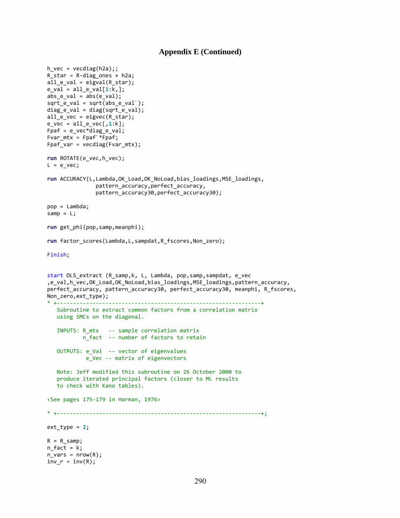
Appendix E (Continued)
290
h_vec = vecdiag(h2a);; R_star = R‐diag_ones + h2a; all_e_val = eigval(R_star); e_val = all_e_val[1:k,]; abs_e_val = abs(e_val); sqrt_e_val = sqrt(abs_e_val`); diag_e_val = diag(sqrt_e_val); all_e_vec = eigvec(R_star); e_vec = all_e_vec[,1:k]; Fpaf = e_vec*diag_e_val; Fvar_mtx = Fpaf`*Fpaf; Fpaf_var = vecdiag(Fvar_mtx); run ROTATE(e_vec,h_vec); L = e_vec; run ACCURACY(L,Lambda,OK_Load,OK_NoLoad,bias_loadings,MSE_loadings, pattern_accuracy,perfect_accuracy, pattern_accuracy30,perfect_accuracy30); pop = Lambda; samp = L; run get_phi(pop,samp,meanphi); run factor_scores(Lambda,L,sampdat,R_fscores,Non_zero); Finish; start OLS_extract (R_samp,k, L, Lambda, pop,samp,sampdat, e_vec ,e_val,h_vec,OK_Load,OK_NoLoad,bias_loadings,MSE_loadings,pattern_accuracy, perfect_accuracy, pattern_accuracy30, perfect_accuracy30, meanphi, R_fscores, Non_zero,ext_type); * +‐‐‐‐‐‐‐‐‐‐‐‐‐‐‐‐‐‐‐‐‐‐‐‐‐‐‐‐‐‐‐‐‐‐‐‐‐‐‐‐‐‐‐‐‐‐‐‐‐‐‐‐‐‐‐‐‐‐‐‐‐‐‐+ Subroutine to extract common factors from a correlation matrix using SMCs on the diagonal. INPUTS: R_mtx ‐‐ sample correlation matrix n_fact ‐‐ number of factors to retain OUTPUTS: e_Val ‐‐ vector of eigenvalues e_Vec ‐‐ matrix of eigenvectors Note: Jeff modified this subroutine on 26 October 2000 to produce iterated principal factors (closer to ML results to check with Kano tables). <See pages 175‐179 in Harman, 1976> * +‐‐‐‐‐‐‐‐‐‐‐‐‐‐‐‐‐‐‐‐‐‐‐‐‐‐‐‐‐‐‐‐‐‐‐‐‐‐‐‐‐‐‐‐‐‐‐‐‐‐‐‐‐‐‐‐‐‐‐‐‐‐‐+; ext_type = 2; R = R_samp; n_fact = k; n_vars = nrow(R); inv_r = inv(R);

Appendix E (Continued)
291
h2a = J(n_vars,1,0); do i = 1 to n_vars; h2a[i,1] = 1‐1/inv_r[i,i]; r[i,i] = h2a[i,1]; end; oldcomm = h2a; change = 1; do until (change< .0001); e_val = eigval(R); e_val = e_val[1:n_fact,]; eVec_orig = eigvec(R); eVec_orig = eVec_orig[,1:n_fact]; e_Vec = J(n_Vars,n_fact,0); do i = 1 to n_Vars; do j = 1 to n_fact; if (e_val[j,1]< 0) then e_val[j,1] = 0; e_vec[i,j] = eVec_orig[i,j]#sqrt(e_val[j,1]); end; end; change = 0; h_vec = h2a; end; run ROTATE(e_vec,h_vec); L = e_vec; run ACCURACY(L,Lambda,OK_Load,OK_NoLoad,bias_loadings,MSE_loadings, pattern_accuracy,perfect_accuracy, pattern_accuracy30,perfect_accuracy30); pop = Lambda; samp = L; run get_phi(pop,samp,meanphi); run factor_scores(Lambda,L,sampdat,R_fscores,Non_zero); finish; /*Maximum Likelihood method adapted from Chen, R. (2003)*/ start mlfa; ext_type = 3; s = r_samp; /* objective function module */ start objfun (x) global(s, k, p, xpsy, sigma, lambda, omega, f); xpsy = diag(1/sqrt(x)); A = xpsy*s*xpsy; Omega = (eigvec(A)) [,1:k]; theta = (eigval(A)) [1:k]; lambda = diag(sqrt(x))*omega*diag(sqrt(abs(theta‐1))); sigma = lambda*t(lambda)+diag(x); f = log(det(sigma))+trace(s*inv(sigma))‐log(det(s))‐p; return(f);

Appendix E (Continued)
292
finish; /* Gradient function module */ start gradfun(x) global(s, sigma); invpsy = inv(diag(x)); g = (vecdiag(invpsy*(sigma‐s)*invpsy))`; return(g); finish; /* starting values for iteration */ p = ncol(s); x = (1‐k/(2#p))#(1/vecdiag(inv(s))); /* Set up Options and Constraints */ option = {0 0 . 4}; con = j(1,p, 0.00001)//j(1,p,.); call nlpqn(rc, xr, "objfun", x, option, con) grd = "gradfun"; r_star = lambda*lambda`; h_vec = vecdiag(r_star); all_e_vec = eigvec(R_star); e_vec = all_e_vec[,1:k]; finish; start mlfa_extract; run mlfa; if rc < 0 then m_rc0 = 1; else m_rc0 = 0; if rc = 3 then m_rc3 = 1; else m_rc3 = 0; if rc = 6 then m_rc6 = 1; else m_rc6 = 0; run ROTATE(e_vec,h_vec); L = e_vec; run ACCURACY(L,Lambda,OK_Load,OK_NoLoad,bias_loadings,MSE_loadings, pattern_accuracy,perfect_accuracy, pattern_accuracy30,perfect_accuracy30); pop = Lambda; samp = L; run get_phi(pop,samp,meanphi); run factor_scores(Lambda,L,sampdat,R_fscores,Non_zero); finish; Do pop_num = 1 to N_pops; * Loop for 10 populations; run Make_PopR(p,k,commun_type,A1,R_pop); Lambda = A1; numr = r_pop[+,+] ‐ p;

Appendix E (Continued)
293
deno = r_pop[+,+]; ratio = numr/deno; f2_pop = (p/(p‐1))*ratio; r2_pop = f2_pop/(1+f2_pop); corr = r_pop; seed1=round(1000000*rannor(0)); *nn = 100000; chg = 1; cycle = 0; corr_tmp = corr; do until (chg = 0); run gendata2a(NN1,seed1,variance,1,0,0,means,corr_tmp,sim_data,p,d_frac); sim_corr = corr(sim_data); resid_m = sim_corr ‐ corr; tot_res = sum(abs(resid_m)); if cycle = 0 then do; best_corr = corr_tmp; best_res = tot_res; end; if cycle > 0 then do; if tot_res < best_res then do; best_corr = corr_tmp; best_res = tot_res; end; end; if tot_res < (.005#(((p‐1)#p)/2)) then CHG = 0; * Convergence!; if cycle > 30 then do; if tot_res < (.01#(((p‐1)#p)/2)) then CHG = 0; * Convergence!; end; if cycle > 200 then CHG = 0; if CHG = 1 then corr_tmp = corr_tmp ‐ resid_m; * adjust template and simulate another large sample; cycle = cycle + 1; if CHG = 0 then do; end; end; Do S_Size = 1 to 4; * Loop for sample sizes; if S_Size = 1 then Sampsize2=100; if S_Size = 2 then Sampsize2=200; if S_Size = 3 then Sampsize2=300; if S_Size = 4 then Sampsize2=1000; Do rep=1 to replicat; * Loop for 1000 Samples; **********************************************************: * Begin data generation *; **********************************************************; seed1=round(1000000*ranuni(0)); nn2 = sampsize2; corr_tmp = best_corr; r_sing = 0;
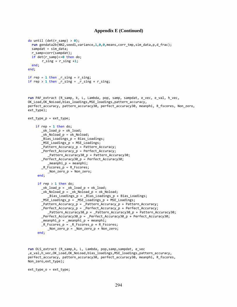
Appendix E (Continued)
294
do until (det(r_samp) > 0); run gendata2b(NN2,seed1,variance,1,0,0,means,corr_tmp,sim_data,p,d_frac); sampdat = sim_data; r_samp=corr(sampdat); if det(r_samp)<=0 then do; r_sing = r_sing +1; end; end; if rep = 1 then _r_sing = r_sing; if rep > 1 then _r_sing = _r_sing + r_sing; run PAF_extract (R_samp, k, L, Lambda, pop, samp, sampdat, e_vec, e_val, h_vec, OK_Load,OK_NoLoad,bias_loadings,MSE_loadings,pattern_accuracy, perfect_accuracy, pattern_accuracy30, perfect_accuracy30, meanphi, R_fscores, Non_zero, ext_type); ext_type_p = ext_type; if rep = 1 then do; _ok_load_p = ok_load; _ok_Noload_p = ok_Noload; _Bias_Loadings_p = Bias_Loadings; _MSE_Loadings_p = MSE_Loadings; _Pattern_Accuracy_p = Pattern_Accuracy; _Perfect_Accuracy_p = Perfect_Accuracy; _Pattern_Accuracy30_p = Pattern_Accuracy30; _Perfect_Accuracy30_p = Perfect_Accuracy30; _meanphi_p = meanphi; _R_Fscores_p = R_Fscores; _Non_zero_p = Non_zero; end; if rep > 1 then do; _ok_load_p = _ok_load_p + ok_load; _ok_Noload_p = _ok_Noload_p + ok_Noload; _Bias_Loadings_p = _Bias_Loadings_p + Bias_Loadings; _MSE_Loadings_p = _MSE_Loadings_p + MSE_Loadings; _Pattern_Accuracy_p = _Pattern_Accuracy_p + Pattern_Accuracy; _Perfect_Accuracy_p = _Perfect_Accuracy_p + Perfect_Accuracy; _Pattern_Accuracy30_p = _Pattern_Accuracy30_p + Pattern_Accuracy30; _Perfect_Accuracy30_p = _Perfect_Accuracy30_p + Perfect_Accuracy30; _meanphi_p = _meanphi_p + meanphi; _R_Fscores_p = _R_Fscores_p + R_Fscores; _Non_zero_p = _Non_zero_p + Non_zero; end; run OLS_extract (R_samp,k, L, Lambda, pop,samp,sampdat, e_vec ,e_val,h_vec,OK_Load,OK_NoLoad,bias_loadings,MSE_loadings,pattern_accuracy, perfect_accuracy, pattern_accuracy30, perfect_accuracy30, meanphi, R_fscores, Non_zero,ext_type); ext_type_o = ext_type;

Appendix E (Continued)
295
if rep = 1 then do; _ok_load_o = ok_load; _ok_Noload_o = ok_Noload; _Bias_Loadings_o = Bias_Loadings; _MSE_Loadings_o = MSE_Loadings; _Pattern_Accuracy_o = Pattern_Accuracy; _Perfect_Accuracy_o = Perfect_Accuracy; _Pattern_Accuracy30_o = Pattern_Accuracy30; _Perfect_Accuracy30_o = Perfect_Accuracy30; _meanphi_o = meanphi; _R_Fscores_o = R_Fscores; _Non_zero_o = Non_zero; end; if rep > 1 then do; _ok_load_o = _ok_load_o + ok_load; _ok_Noload_o = _ok_Noload_o + ok_Noload; _Bias_Loadings_o = _Bias_Loadings_o + Bias_Loadings; _MSE_Loadings_o = _MSE_Loadings_o + MSE_Loadings; _Pattern_Accuracy_o = _Pattern_Accuracy_o + Pattern_Accuracy; _Perfect_Accuracy_o = _Perfect_Accuracy_o + Perfect_Accuracy; _Pattern_Accuracy30_o = _Pattern_Accuracy30_o + Pattern_Accuracy30; _Perfect_Accuracy30_o = _Perfect_Accuracy30_o + Perfect_Accuracy30; _meanphi_o = _meanphi_o + meanphi; _R_Fscores_o = _R_Fscores_o + R_Fscores; _Non_zero_o = _Non_zero_o + Non_zero; end; run mlfa_extract; ext_type_m = ext_type; if rep = 1 then do; _m_rc0 = m_rc0; _m_rc3 = m_rc3; _m_rc6 = m_rc6; _ok_load_m = ok_load; _ok_Noload_m = ok_Noload; _Bias_Loadings_m = Bias_Loadings; _MSE_Loadings_m = MSE_Loadings; _Pattern_Accuracy_m = Pattern_Accuracy; _Perfect_Accuracy_m = Perfect_Accuracy; _Pattern_Accuracy30_m = Pattern_Accuracy30; _Perfect_Accuracy30_m = Perfect_Accuracy30; _meanphi_m = meanphi; _R_Fscores_m = R_Fscores; _Non_zero_m = Non_zero; end; if rep > 1 then do; _m_rc0 = _m_rc0 + m_rc0; _m_rc3 = _m_rc3 + m_rc3; _m_rc6 = _m_rc6 + m_rc6; _ok_load_m = _ok_load_m + ok_load; _ok_Noload_m = _ok_Noload_m + ok_Noload; _Bias_Loadings_m = _Bias_Loadings_m + Bias_Loadings; _MSE_Loadings_m = _MSE_Loadings_m + MSE_Loadings;

Appendix E (Continued)
296
_Pattern_Accuracy_m = _Pattern_Accuracy_m + Pattern_Accuracy; _Perfect_Accuracy_m = _Perfect_Accuracy_m + Perfect_Accuracy; _Pattern_Accuracy30_m = _Pattern_Accuracy30_m + Pattern_Accuracy30; _Perfect_Accuracy30_m = _Perfect_Accuracy30_m + Perfect_Accuracy30; _meanphi_m = _meanphi_m + meanphi; _R_Fscores_m = _R_Fscores_m + R_Fscores; _Non_zero_m = _Non_zero_m + Non_zero; end; if rep = 1 then nsamples = 1; if rep > 1 then nsamples = nsamples +1; end; *End Replications Loop*; _ok_load_p = _ok_load_p/NSamples; _ok_Noload_p = _ok_Noload_p/NSamples; _Bias_Loadings_p = _BIas_Loadings_p/NSamples; _MSE_Loadings_p = _MSE_Loadings_p/NSamples; _Pattern_Accuracy_p = _Pattern_Accuracy_p/NSamples; _Perfect_Accuracy_p = _Perfect_Accuracy_p/NSamples; _Pattern_Accuracy30_p = _Pattern_Accuracy30_p/NSamples; _Perfect_Accuracy30_p = _Perfect_Accuracy30_p/NSamples; _meanphi_p = _meanphi_p/NSamples; _R_Fscores_p = _R_Fscores_p/NSamples; _Non_zero_p = _Non_zero_p/NSamples; _ok_load_o = _ok_load_o/NSamples; _ok_Noload_o = _ok_Noload_o/NSamples; _Bias_Loadings_o = _BIas_Loadings_o/NSamples; _MSE_Loadings_o = _MSE_Loadings_o/NSamples; _Pattern_Accuracy_o = _Pattern_Accuracy_o/NSamples; _Pefect_Accuracy_o = _Perfect_Accuracy_o/NSamples; _Pattern_Accuracy30_o = _Pattern_Accuracy30_o/NSamples; _Perfect_Accuracy30_o = _Perfect_Accuracy30_o/NSamples; _meanphi_o = _meanphi_o/NSamples; _R_Fscores_o = _R_Fscores_o/NSamples; _Non_zero_o = _Non_zero_o/NSamples; _m_rc0 = _m_rc0; _m_rc3 = _m_rc3; _m_rc6 = _m_rc6; _ok_load_m = _ok_load_m/NSamples; _ok_Noload_m = _ok_Noload_m/NSamples; _Bias_Loadings_m = _BIas_Loadings_m/NSamples; _MSE_Loadings_m = _MSE_Loadings_m/NSamples; _Pattern_Accuracy_m = _Pattern_Accuracy_m/NSamples; _Perfect_Accuracy_m = _Perfect_Accuracy_m/NSamples; _Pattern_Accuracy30_m = _Pattern_Accuracy30_m/NSamples; _Perfect_Accuracy30_m = _Perfect_Accuracy30_m/NSamples; _meanphi_m = _meanphi_m/NSamples; _R_Fscores_m = _R_Fscores_m/NSamples; _Non_zero_m = _Non_zero_m/NSamples; _r_sing = _r_sing; print Sampsize2 commun_type d_frac k p; print ' ';
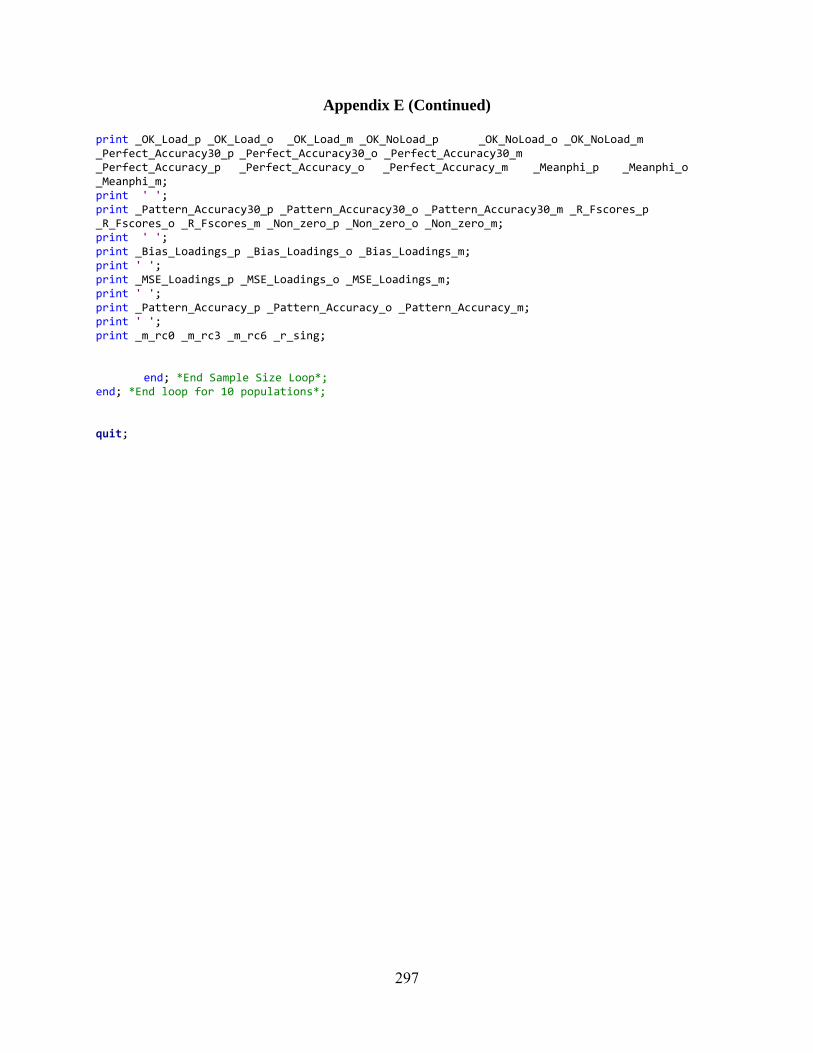
Appendix E (Continued)
297
print _OK_Load_p _OK_Load_o _OK_Load_m _OK_NoLoad_p _OK_NoLoad_o _OK_NoLoad_m _Perfect_Accuracy30_p _Perfect_Accuracy30_o _Perfect_Accuracy30_m _Perfect_Accuracy_p _Perfect_Accuracy_o _Perfect_Accuracy_m _Meanphi_p _Meanphi_o _Meanphi_m; print ' '; print _Pattern_Accuracy30_p _Pattern_Accuracy30_o _Pattern_Accuracy30_m _R_Fscores_p _R_Fscores_o _R_Fscores_m _Non_zero_p _Non_zero_o _Non_zero_m; print ' '; print _Bias_Loadings_p _Bias_Loadings_o _Bias_Loadings_m; print ' '; print _MSE_Loadings_p _MSE_Loadings_o _MSE_Loadings_m; print ' '; print _Pattern_Accuracy_p _Pattern_Accuracy_o _Pattern_Accuracy_m; print ' '; print _m_rc0 _m_rc3 _m_rc6 _r_sing;
end; *End Sample Size Loop*; end; *End loop for 10 populations*; quit;
Appendix F
298
Analysis Program: SAS, IML©
data a; infile 'C:\kcoughlin document\dissertation\data files\refined merged data 07242012.lst' lrecl = 256 missover pad; input test_var $ 1 ‐ 256 @; rec_num = _n_; file = 'kcoughlin'; if index(test_var, 'SAMPSIZE2') ^=0 OR index(test_var, 'Sampsize2') ^=0 then record_type = 'Record 10'; if index(test_var, '_OK_LOAD_P') ^=0 OR index(test_var, '_ok_load_p')^=0 then record_type = 'Record 20'; if index(test_var, '_PATTERN_ACCURACY30_P') ^=0 OR index(test_var, '_Pattern_Accuracy30_p')^=0 then record_type = 'Record 30'; if index(test_var, '_BIAS_LOADINGS_P') ^=0 OR index(test_var, '_Bias_Loadings_p') ^=0 then record_type = 'Record 40'; if index(test_var, '_BIAS_LOADINGS_M') ^=0 OR index(test_var, '_Bias_Loadings_m') ^=0 then record_type = 'Record 42'; if index(test_var, '_MSE_LOADINGS_P') ^=0 OR index(test_var, '_MSE_Loadings_p') ^=0 then record_type = 'Record 50'; if index(test_var, '_MSE_LOADINGS_M') ^=0 OR index(test_var, '_MSE_Loadings_m') ^=0 then record_type = 'Record 52'; if index(test_var, '_PATTERN_ACCURACY_P') ^=0 OR index(test_var, '_Pattern_Accuracy_p') ^=0 then record_type = 'Record 60'; if index(test_var, '_PATTERN_ACCURACY_M') ^=0 OR index(test_var, '_Pattern_Accuracy_m') ^=0 then record_type = 'Record 62'; if index(test_var, '_M_RC0') ^=0 OR index(test_var, '_m_rc0') ^=0 then record_type = 'Record 70'; if record_type = 'Record 10' then do; input @1 dummy 1. Sampsize2 Commun_type2 d_frac2 k2 p2; if D_FRAC2 ne . then do; P = P2; K = K2; COMMUN_TYPE = COMMUN_TYPE2; D_FRAC = D_FRAC2; SAMPSIZE = SAMPSIZE2; end; end; * retain Sampsize2 Commun_type d_frac k p; if record_type = 'Record 20' then do; input @1 dummy 1. _ok_load_p _ok_load_o _ok_load_m _ok_Noload_p _ok_Noload_o _ok_Noload_m _Perfect_Accuracy30_p _Perfect_Accuracy30_o _Perfect_Accuracy30_m _Perfect_Accuracy_p _Perfect_Accuracy_o _Perfect_Accuracy_m _meanphi_p _meanphi_o _meanphi_m; end;
Appendix F (Continued)
299
if record_type = 'Record 30' then do; input @1 dummy 1. _Pattern_Accuracy30_p _Pattern_Accuracy30_o _Pattern_Accuracy30_m _R_Fscores_p _R_Fscores_o _R_Fscores_m _Non_zero_p _Non_zero_o _Non_zero_m; end; if record_type = 'Record 40' and k = 8 then do; input @1 dummy 1. _Bias_Loadings_p1 _Bias_Loadings_p2 _Bias_Loadings_p3 _Bias_Loadings_p4 _Bias_Loadings_p5 _Bias_Loadings_p6 _Bias_Loadings_p7 _Bias_Loadings_p8 _Bias_Loadings_o1 _Bias_Loadings_o2 _Bias_Loadings_o3 _Bias_Loadings_o4; end; if record_type = 'Record 42' and k = 2 then do; input @1 dummy 1. _Bias_Loadings_p1 _Bias_Loadings_p2 _Bias_Loadings_o1 _Bias_Loadings_o2 _Bias_Loadings_m1 _Bias_Loadings_m2; end; if record_type = 'Record 42' and k = 4 then do; input @1 dummy 1. _Bias_Loadings_p1 _Bias_Loadings_p2 _Bias_Loadings_p3 _Bias_Loadings_p4 _Bias_Loadings_o1 _Bias_Loadings_o2 _Bias_Loadings_o3 _Bias_Loadings_o4 _Bias_Loadings_m1 _Bias_Loadings_m2 _Bias_Loadings_m3 _Bias_Loadings_m4; end; if record_type = 'Record 42' and k = 8 then do; input @1 dummy 1. _Bias_Loadings_o5 _Bias_Loadings_o6 _Bias_Loadings_o7 _Bias_Loadings_o8 _Bias_Loadings_m1 _Bias_Loadings_m2 _Bias_Loadings_m3 _Bias_Loadings_m4 _Bias_Loadings_m5 _Bias_Loadings_m6 _Bias_Loadings_m7 _Bias_Loadings_m8; end; if record_type = 'Record 50' and k = 8 then do; input @1 dummy 1. _MSE_Loadings_p1 _MSE_Loadings_p2 _MSE_Loadings_p3 _MSE_Loadings_p4 _MSE_Loadings_p5 _MSE_Loadings_p6 _MSE_Loadings_p7 _MSE_Loadings_p8 _MSE_Loadings_o1 _MSE_Loadings_o2 _MSE_Loadings_o3 _MSE_Loadings_o4; end; if record_type = 'Record 52' and k = 2 then do; input @1 dummy 1. _MSE_Loadings_p1 _MSE_Loadings_p2 _MSE_Loadings_o1 _MSE_Loadings_o2 _MSE_Loadings_m1 _MSE_Loadings_m2; end; if record_type = 'Record 52' and k = 4 then do; input @1 dummy 1. _MSE_Loadings_p1 _MSE_Loadings_p2 _MSE_Loadings_p3 _MSE_Loadings_p4 _MSE_Loadings_o1 _MSE_Loadings_o2 _MSE_Loadings_o3 _MSE_Loadings_o4 _MSE_Loadings_m1 _MSE_Loadings_m2 _MSE_Loadings_m3 _MSE_Loadings_m4; end; if record_type = 'Record 52' and k = 8 then do; input @1 dummy 1. _MSE_Loadings_o5 _MSE_Loadings_o6 _MSE_Loadings_o7 _MSE_Loadings_o8
Appendix F (Continued)
300
_MSE_Loadings_m1 _MSE_Loadings_m2 _MSE_Loadings_m3 _MSE_Loadings_m4 _MSE_Loadings_m5 _MSE_Loadings_m6 _MSE_Loadings_m7 _MSE_Loadings_m8; end; if record_type = 'Record 60' and k = 8 then do; input @1 dummy 1. _Pattern_Accuracy_p1 _Pattern_Accuracy_p2 _Pattern_Accuracy_p3 _Pattern_Accuracy_p4 _Pattern_Accuracy_p5 _Pattern_Accuracy_p6 _Pattern_Accuracy_p7 _Pattern_Accuracy_p8 _Pattern_Accuracy_o1 _Pattern_Accuracy_o2 _Pattern_Accuracy_o3 _Pattern_Accuracy_o4; end; if record_type = 'Record 62' and k = 2 then do; input @1 dummy 1. _Pattern_Accuracy_p1 _Pattern_Accuracy_p2 _Pattern_Accuracy_o1 _Pattern_Accuracy_o2 _Pattern_Accuracy_m1 _Pattern_Accuracy_m2; end; if record_type = 'Record 62' and k = 4 then do; input @1 dummy 1. _Pattern_Accuracy_p1 _Pattern_Accuracy_p2 _Pattern_Accuracy_p3 _Pattern_Accuracy_p4 _Pattern_Accuracy_o1 _Pattern_Accuracy_o2 _Pattern_Accuracy_o3 _Pattern_Accuracy_o4 _Pattern_Accuracy_m1 _Pattern_Accuracy_m2 _Pattern_Accuracy_m3 _Pattern_Accuracy_m4; end; if record_type = 'Record 62' and k = 8 then do; input @1 dummy 1. _Pattern_Accuracy_o5 _Pattern_Accuracy_o6 _Pattern_Accuracy_o7 _Pattern_Accuracy_o8 _Pattern_Accuracy_m1 _Pattern_Accuracy_m2 _Pattern_Accuracy_m3 _Pattern_Accuracy_m4 _Pattern_Accuracy_m5 _Pattern_Accuracy_m6 _Pattern_Accuracy_m7 _Pattern_Accuracy_m8; end; if record_type = 'Record 70' then do; input @1 dummy 1. _m_rc0 _m_rc3 _m_rc6; end; retain record_type Sampsize Commun_type d_frac k p; drop test_var; if Sampsize = . and _ok_load_p =. and _Pattern_Accuracy30_p = . and _Bias_Loadings_p1 = . and _MSE_Loadings_p1 = . and _Pattern_Accuracy_p1 = . and _m_rc0 = . then delete; data a1; set a; _perfect_accuracy_o = _perfect_accuracy_o/10000; proc sort data = a1; by Sampsize Commun_type d_frac k p; proc means noprint data = a1; by Sampsize Commun_type d_frac k p; var _ok_load_p _ok_load_o _ok_load_m _ok_Noload_p _ok_Noload_o _ok_Noload_m _Perfect_Accuracy30_p _Perfect_Accuracy30_o _Perfect_Accuracy30_m _Perfect_Accuracy_p _Perfect_Accuracy_o _Perfect_Accuracy_m _meanphi_p _meanphi_o _meanphi_m _Pattern_Accuracy30_p _Pattern_Accuracy30_o _Pattern_Accuracy30_m _R_Fscores_p _R_Fscores_o _R_Fscores_m _Non_zero_p _Non_zero_o _Non_zero_m
Appendix F (Continued)
301
_Bias_Loadings_p1 _Bias_Loadings_p2 _Bias_Loadings_p3 _Bias_Loadings_p4 _Bias_Loadings_p5 _Bias_Loadings_p6 _Bias_Loadings_p7 _Bias_Loadings_p8 _Bias_Loadings_o1 _Bias_Loadings_o2 _Bias_Loadings_o3 _Bias_Loadings_o4 _Bias_Loadings_o5 _Bias_Loadings_o6 _Bias_Loadings_o7 _Bias_Loadings_o8 _Bias_Loadings_m1 _Bias_Loadings_m2 _Bias_Loadings_m3 _Bias_Loadings_m4 _Bias_Loadings_m5 _Bias_Loadings_m6 _Bias_Loadings_m7 _Bias_Loadings_m8 _MSE_Loadings_p1 _MSE_Loadings_p2 _MSE_Loadings_p3 _MSE_Loadings_p4 _MSE_Loadings_p5 _MSE_Loadings_p6 _MSE_Loadings_p7 _MSE_Loadings_p8 _MSE_Loadings_o1 _MSE_Loadings_o2 _MSE_Loadings_o3 _MSE_Loadings_o4 _MSE_Loadings_o5 _MSE_Loadings_o6 _MSE_Loadings_o7 _MSE_Loadings_o8 _MSE_Loadings_m1 _MSE_Loadings_m2 _MSE_Loadings_m3 _MSE_Loadings_m4 _MSE_Loadings_m5 _MSE_Loadings_m6 _MSE_Loadings_m7 _MSE_Loadings_m8 _Pattern_Accuracy_p1 _Pattern_Accuracy_p2 _Pattern_Accuracy_p3 _Pattern_Accuracy_p4 _Pattern_Accuracy_p5 _Pattern_Accuracy_p6 _Pattern_Accuracy_p7 _Pattern_Accuracy_p8 _Pattern_Accuracy_o1 _Pattern_Accuracy_o2 _Pattern_Accuracy_o3 _Pattern_Accuracy_o4 _Pattern_Accuracy_o5 _Pattern_Accuracy_o6 _Pattern_Accuracy_o7 _Pattern_Accuracy_o8 _Pattern_Accuracy_m1 _Pattern_Accuracy_m2 _Pattern_Accuracy_m3 _Pattern_Accuracy_m4 _Pattern_Accuracy_m5 _Pattern_Accuracy_m6 _Pattern_Accuracy_m7 _Pattern_Accuracy_m8 _m_rc0 _m_rc3 _m_rc6; output out = b mean = ; /*descriptive statistics*/ data c; set b; _bias_loadings_p = mean (of _Bias_Loadings_p1 ‐ _Bias_Loadings_p8); _bias_loadings_o = mean (of _Bias_Loadings_o1 ‐ _Bias_Loadings_o8); _bias_loadings_m = mean (of _Bias_Loadings_m1 ‐ _Bias_Loadings_m8); _mse_leadings_p = mean (of _MSE_Loadings_p1 ‐ _MSE_Loadings_p8); _mse_leadings_o = mean (of _MSE_Loadings_o1 ‐ _MSE_Loadings_o8); _mse_leadings_m = mean (of _MSE_Loadings_m1 ‐ _MSE_Loadings_m8); _pattern_accuracy_p = mean (of _Pattern_Accuracy_p1 ‐ _Pattern_Accuracy_p8); _pattern_accuracy_o = mean (of _Pattern_Accuracy_o1 ‐ _Pattern_Accuracy_o8); _pattern_accuracy_m = mean (of _Pattern_Accuracy_m1 ‐ _Pattern_Accuracy_m8); proc means data = c; var _ok_load_p _ok_load_o _ok_load_m _Perfect_Accuracy30_p _Perfect_Accuracy30_o _Perfect_Accuracy30_m _Perfect_Accuracy_p _Perfect_Accuracy_o _Perfect_Accuracy_m _meanphi_p _meanphi_o _meanphi_m _Pattern_Accuracy30_p _Pattern_Accuracy30_o _Pattern_Accuracy30_m _R_Fscores_p _R_Fscores_o _R_Fscores_m _Non_zero_p _Non_zero_o _Non_zero_m _bias_loadings_p _bias_loadings_o _bias_loadings_m _mse_leadings_p _mse_leadings_o _mse_leadings_m _pattern_accuracy_p _pattern_accuracy_o _pattern_accuracy_m _m_rc0 _m_rc3 _m_rc6; proc univariate normal data = c; var _ok_load_p _ok_load_o _ok_load_m _Perfect_Accuracy30_p _Perfect_Accuracy30_o _Perfect_Accuracy30_m _Perfect_Accuracy_p _Perfect_Accuracy_o _Perfect_Accuracy_m _meanphi_p _meanphi_o _meanphi_m _Pattern_Accuracy30_p _Pattern_Accuracy30_o _Pattern_Accuracy30_m _R_Fscores_p _R_Fscores_o _R_Fscores_m _Non_zero_p _Non_zero_o _Non_zero_m _bias_loadings_p _bias_loadings_o _bias_loadings_m _mse_leadings_p _mse_leadings_o _mse_leadings_m _pattern_accuracy_p _pattern_accuracy_o _pattern_accuracy_m

Appendix F (Continued)
302
_m_rc0 _m_rc3 _m_rc6; /*repeated measures analyses*/ proc glm data = c; class k p Sampsize commun_type d_frac; model _ok_load_p _ok_load_o _ok_load_m = k | p | Sampsize | commun_type | d_frac @2; repeated method 3/printe; ods output ModelANOVA = c1; means k*p p*commun_type k*d_frac k*commun_type; proc iml; use c1; read all var {SS} where (Source = 'K' & DEPENDENT = 'BetweenSubjects') into SS_K; read all var {SS} where (Source = 'P' & DEPENDENT = 'BetweenSubjects') into SS_P; read all var {SS} where (Source = 'SAMPSIZE' & DEPENDENT = 'BetweenSubjects') into SS_SAMP; read all var {SS} where (Source = 'COMMUN_TYPE' & DEPENDENT = 'BetweenSubjects') into SS_COMM; read all var {SS} where (Source = 'D_FRAC' & DEPENDENT = 'BetweenSubjects') into SS_DFRAC; read all var {SS} where (Source = 'K*P' & DEPENDENT = 'BetweenSubjects') into SS_K_P; read all var {SS} where (Source = 'K*SAMPSIZE' & DEPENDENT = 'BetweenSubjects') into SS_K_SAMP; read all var {SS} where (Source = 'K*COMMUN_TYPE' & DEPENDENT = 'BetweenSubjects') into SS_K_COMM; read all var {SS} where (Source = 'K*D_FRAC' & DEPENDENT = 'BetweenSubjects') into SS_K_DFRAC; read all var {SS} where (Source = 'P*SAMPSIZE' & DEPENDENT = 'BetweenSubjects') into SS_P_SAMP; read all var {SS} where (Source = 'P*COMMUN_TYPE' & DEPENDENT = 'BetweenSubjects') into SS_P_COMM; read all var {SS} where (Source = 'P*D_FRAC' & DEPENDENT = 'BetweenSubjects') into SS_P_DFRAC; read all var {SS} where (Source = 'SAMPSIZE*COMMUN_TYPE' & DEPENDENT = 'BetweenSubjects') into SS_SAMP_COMM; read all var {SS} where (Source = 'SAMPSIZE*D_FRAC' & DEPENDENT = 'BetweenSubjects') into SS_SAMP_DFRAC; read all var {SS} where (Source = 'COMMUN_TYPE*D_FRAC' & DEPENDENT = 'BetweenSubjects') into SS_COMM_DFRAC; read all var {SS} where (Source = 'Error' & DEPENDENT = 'BetweenSubjects') into SS_Error_Btwn; read all var {SS} where (Source = 'method' & DEPENDENT = 'WithinSubject') into SS_Method; read all var {SS} where (Source = 'method*K' & DEPENDENT = 'WithinSubject') into SS_Method_K; read all var {SS} where (Source = 'method*P' & DEPENDENT = 'WithinSubject') into SS_Method_P; read all var {SS} where (Source = 'method*SAMPSIZE' & DEPENDENT = 'WithinSubject') into SS_Method_SAMP; read all var {SS} where (Source = 'method*COMMUN_TYPE' & DEPENDENT = 'WithinSubject') into SS_Method_COMM; read all var {SS} where (Source = 'method*D_FRAC' & DEPENDENT = 'WithinSubject') into SS_Method_DFRAC; read all var {SS} where (Source = 'method*K*P' & DEPENDENT = 'WithinSubject') into SS_Method_K_P; read all var {SS} where (Source = 'method*K*SAMPSIZE' & DEPENDENT = 'WithinSubject') into SS_Method_K_SAMP; read all var {SS} where (Source = 'method*K*COMMUN_TYPE' & DEPENDENT = 'WithinSubject') into SS_Method_K_COMM; read all var {SS} where (Source = 'method*K*D_FRAC' & DEPENDENT = 'WithinSubject') into SS_Method_K_DFRAC; read all var {SS} where (Source = 'method*P*SAMPSIZE' & DEPENDENT = 'WithinSubject') into SS_Method_P_SAMP;
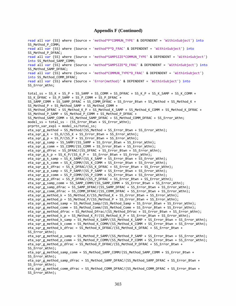
Appendix F (Continued)
303
read all var {SS} where (Source = 'method*P*COMMUN_TYPE' & DEPENDENT = 'WithinSubject') into SS_Method_P_COMM; read all var {SS} where (Source = 'method*P*D_FRAC' & DEPENDENT = 'WithinSubject') into SS_Method_P_DFRAC; read all var {SS} where (Source = 'method*SAMPSIZE*COMMUN_TYPE' & DEPENDENT = 'WithinSubject') into SS_Method_SAMP_COMM; read all var {SS} where (Source = 'method*SAMPSIZE*D_FRAC' & DEPENDENT = 'WithinSubject') into SS_Method_SAMP_DFRAC; read all var {SS} where (Source = 'method*COMMUN_TYPE*D_FRAC' & DEPENDENT = 'WithinSubject') into SS_Method_COMM_DFRAC; read all var {SS} where (Source = 'Error(method)' & DEPENDENT = 'WithinSubject') into SS_Error_Wthn; total_ss = SS_K + SS_P + SS_SAMP + SS_COMM + SS_DFRAC + SS_K_P + SS_K_SAMP + SS_K_COMM + SS_K_DFRAC + SS_P_SAMP + SS_P_COMM + SS_P_DFRAC + SS_SAMP_COMM + SS_SAMP_DFRAC + SS_COMM_DFRAC + SS_Error_Btwn + SS_Method + SS_Method_K + SS_Method_P + SS_Method_SAMP + SS_Method_COMM + SS_Method_DFRAC + SS_Method_K_P + SS_Method_K_SAMP + SS_Method_K_COMM + SS_Method_K_DFRAC + SS_Method_P_SAMP + SS_Method_P_COMM + SS_Method_P_DFRAC + SS_Method_SAMP_COMM + SS_Method_SAMP_DFRAC + SS_Method_COMM_DFRAC + SS_Error_Wthn; model_ss = total_ss ‐ (SS_Error_Btwn + SS_Error_Wthn); prprtn_var_expl = model_ss/total_ss; eta_sqr_g_method = SS_Method/(SS_Method + SS_Error_Btwn + SS_Error_Wthn); eta_sqr_g_k = SS_K/(SS_K + SS_Error_Btwn + SS_Error_Wthn); eta_sqr_g_p = SS_P/(SS_P + SS_Error_Btwn + SS_Error_Wthn); eta_sqr_g_samp = SS_SAMP/(SS_SAMP + SS_Error_Btwn + SS_Error_Wthn); eta_sqr_g_comm = SS_COMM/(SS_COMM + SS_Error_Btwn + SS_Error_Wthn); eta_sqr_g_dfrac = SS_DFRAC/(SS_DFRAC + SS_Error_Btwn + SS_Error_Wthn); eta_sqr_g_k_p = SS_K_P/(SS_K_P + SS_Error_Btwn + SS_Error_Wthn); eta_sqr_g_k_samp = SS_K_SAMP/(SS_K_SAMP + SS_Error_Btwn + SS_Error_Wthn); eta_sqr_g_k_comm = SS_K_COMM/(SS_K_COMM + SS_Error_Btwn + SS_Error_Wthn); eta_sqr_g_k_dfrac = SS_K_DFRAC/(SS_K_DFRAC + SS_Error_Btwn + SS_Error_Wthn); eta_sqr_g_p_samp = SS_P_SAMP/(SS_P_SAMP + SS_Error_Btwn + SS_Error_Wthn); eta_sqr_g_p_comm = SS_P_COMM/(SS_P_COMM + SS_Error_Btwn + SS_Error_Wthn); eta_sqr_g_p_dfrac = SS_P_DFRAC/(SS_P_DFRAC + SS_Error_Btwn + SS_Error_Wthn); eta_sqr_g_samp_comm = SS_SAMP_COMM/(SS_SAMP_COMM + SS_Error_Btwn + SS_Error_Wthn); eta_sqr_g_samp_dfrac = SS_SAMP_DFRAC/(SS_SAMP_DFRAC + SS_Error_Btwn + SS_Error_Wthn); eta_sqr_g_comm_dfrac = SS_COMM_DFRAC/(SS_COMM_DFRAC + SS_Error_Btwn + SS_Error_Wthn); eta_sqr_g_method_k = SS_Method_K/(SS_Method_K + SS_Error_Btwn + SS_Error_Wthn); eta_sqr_g_method_p = SS_Method_P/(SS_Method_P + SS_Error_Btwn + SS_Error_Wthn); eta_sqr_g_method_samp = SS_Method_Samp/(SS_Method_Samp + SS_Error_Btwn + SS_Error_Wthn); eta_sqr_g_method_comm = SS_Method_Comm/(SS_Method_Comm + SS_Error_Btwn + SS_Error_Wthn); eta_sqr_g_method_dfrac = SS_Method_Dfrac/(SS_Method_Dfrac + SS_Error_Btwn + SS_Error_Wthn); eta_sqr_g_method_k_p = SS_Method_K_P/(SS_Method_K_P + SS_Error_Btwn + SS_Error_Wthn); eta_sqr_g_method_k_samp = SS_Method_K_SAMP/(SS_Method_K_SAMP + SS_Error_Btwn + SS_Error_Wthn); eta_sqr_g_method_k_comm = SS_Method_K_COMM/(SS_Method_K_COMM + SS_Error_Btwn + SS_Error_Wthn); eta_sqr_g_method_k_dfrac = SS_Method_K_DFRAC/(SS_Method_K_DFRAC + SS_Error_Btwn + SS_Error_Wthn); eta_sqr_g_method_p_samp = SS_Method_P_SAMP/(SS_Method_P_SAMP + SS_Error_Btwn + SS_Error_Wthn); eta_sqr_g_method_p_comm = SS_Method_P_COMM/(SS_Method_P_COMM + SS_Error_Btwn + SS_Error_Wthn); eta_sqr_g_method_p_dfrac = SS_Method_P_DFRAC/(SS_Method_P_DFRAC + SS_Error_Btwn + SS_Error_Wthn); eta_sqr_g_method_samp_comm = SS_Method_SAMP_COMM/(SS_Method_SAMP_COMM + SS_Error_Btwn + SS_Error_Wthn); eta_sqr_g_method_samp_dfrac = SS_Method_SAMP_DFRAC/(SS_Method_SAMP_DFRAC + SS_Error_Btwn + SS_Error_Wthn); eta_sqr_g_method_comm_dfrac = SS_Method_COMM_DFRAC/(SS_Method_COMM_DFRAC + SS_Error_Btwn + SS_Error_Wthn);
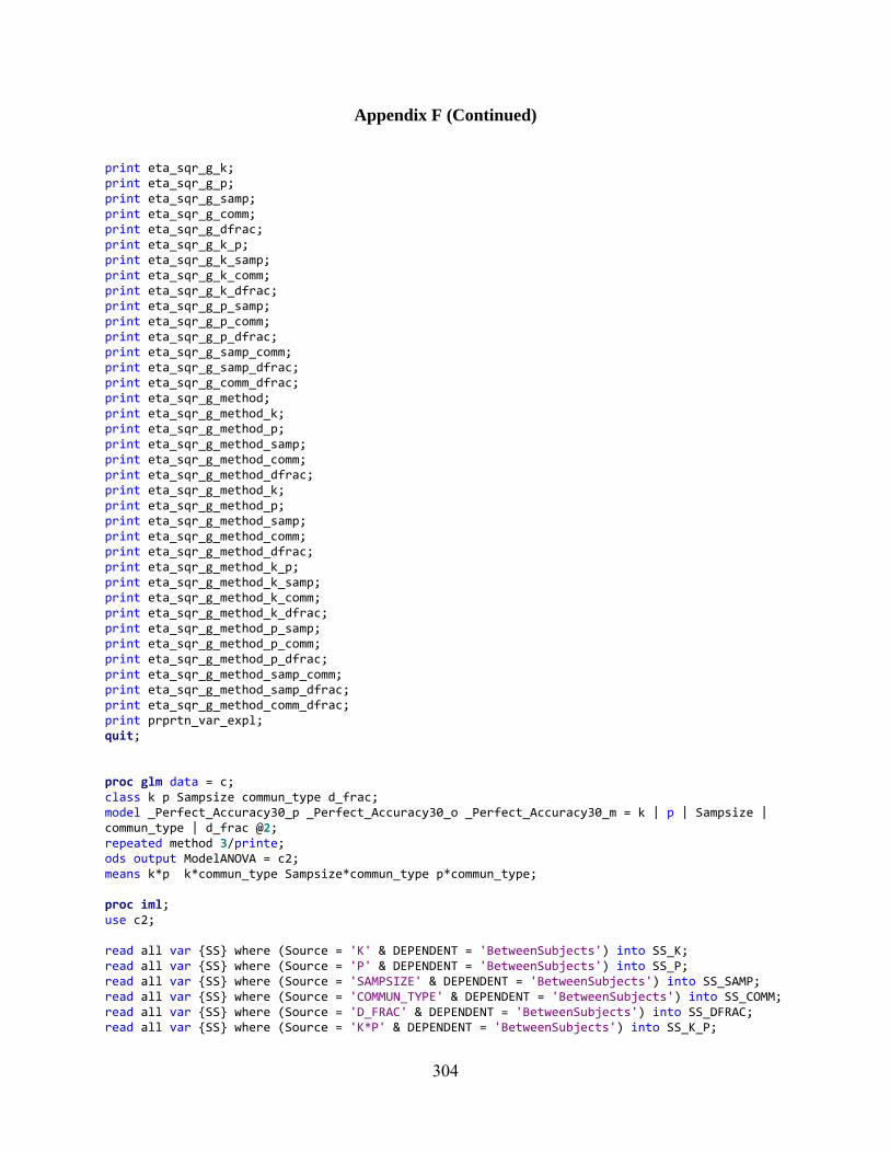
Appendix F (Continued)
304
print eta_sqr_g_k; print eta_sqr_g_p; print eta_sqr_g_samp; print eta_sqr_g_comm; print eta_sqr_g_dfrac; print eta_sqr_g_k_p; print eta_sqr_g_k_samp; print eta_sqr_g_k_comm; print eta_sqr_g_k_dfrac; print eta_sqr_g_p_samp; print eta_sqr_g_p_comm; print eta_sqr_g_p_dfrac; print eta_sqr_g_samp_comm; print eta_sqr_g_samp_dfrac; print eta_sqr_g_comm_dfrac; print eta_sqr_g_method; print eta_sqr_g_method_k; print eta_sqr_g_method_p; print eta_sqr_g_method_samp; print eta_sqr_g_method_comm; print eta_sqr_g_method_dfrac; print eta_sqr_g_method_k; print eta_sqr_g_method_p; print eta_sqr_g_method_samp; print eta_sqr_g_method_comm; print eta_sqr_g_method_dfrac; print eta_sqr_g_method_k_p; print eta_sqr_g_method_k_samp; print eta_sqr_g_method_k_comm; print eta_sqr_g_method_k_dfrac; print eta_sqr_g_method_p_samp; print eta_sqr_g_method_p_comm; print eta_sqr_g_method_p_dfrac; print eta_sqr_g_method_samp_comm; print eta_sqr_g_method_samp_dfrac; print eta_sqr_g_method_comm_dfrac; print prprtn_var_expl; quit; proc glm data = c; class k p Sampsize commun_type d_frac; model _Perfect_Accuracy30_p _Perfect_Accuracy30_o _Perfect_Accuracy30_m = k | p | Sampsize | commun_type | d_frac @2; repeated method 3/printe; ods output ModelANOVA = c2; means k*p k*commun_type Sampsize*commun_type p*commun_type; proc iml; use c2; read all var {SS} where (Source = 'K' & DEPENDENT = 'BetweenSubjects') into SS_K; read all var {SS} where (Source = 'P' & DEPENDENT = 'BetweenSubjects') into SS_P; read all var {SS} where (Source = 'SAMPSIZE' & DEPENDENT = 'BetweenSubjects') into SS_SAMP; read all var {SS} where (Source = 'COMMUN_TYPE' & DEPENDENT = 'BetweenSubjects') into SS_COMM; read all var {SS} where (Source = 'D_FRAC' & DEPENDENT = 'BetweenSubjects') into SS_DFRAC; read all var {SS} where (Source = 'K*P' & DEPENDENT = 'BetweenSubjects') into SS_K_P;

Appendix F (Continued)
305
read all var {SS} where (Source = 'K*SAMPSIZE' & DEPENDENT = 'BetweenSubjects') into SS_K_SAMP; read all var {SS} where (Source = 'K*COMMUN_TYPE' & DEPENDENT = 'BetweenSubjects') into SS_K_COMM; read all var {SS} where (Source = 'K*D_FRAC' & DEPENDENT = 'BetweenSubjects') into SS_K_DFRAC; read all var {SS} where (Source = 'P*SAMPSIZE' & DEPENDENT = 'BetweenSubjects') into SS_P_SAMP; read all var {SS} where (Source = 'P*COMMUN_TYPE' & DEPENDENT = 'BetweenSubjects') into SS_P_COMM; read all var {SS} where (Source = 'P*D_FRAC' & DEPENDENT = 'BetweenSubjects') into SS_P_DFRAC; read all var {SS} where (Source = 'SAMPSIZE*COMMUN_TYPE' & DEPENDENT = 'BetweenSubjects') into SS_SAMP_COMM; read all var {SS} where (Source = 'SAMPSIZE*D_FRAC' & DEPENDENT = 'BetweenSubjects') into SS_SAMP_DFRAC; read all var {SS} where (Source = 'COMMUN_TYPE*D_FRAC' & DEPENDENT = 'BetweenSubjects') into SS_COMM_DFRAC; read all var {SS} where (Source = 'Error' & DEPENDENT = 'BetweenSubjects') into SS_Error_Btwn; read all var {SS} where (Source = 'method' & DEPENDENT = 'WithinSubject') into SS_Method; read all var {SS} where (Source = 'method*K' & DEPENDENT = 'WithinSubject') into SS_Method_K; read all var {SS} where (Source = 'method*P' & DEPENDENT = 'WithinSubject') into SS_Method_P; read all var {SS} where (Source = 'method*SAMPSIZE' & DEPENDENT = 'WithinSubject') into SS_Method_SAMP; read all var {SS} where (Source = 'method*COMMUN_TYPE' & DEPENDENT = 'WithinSubject') into SS_Method_COMM; read all var {SS} where (Source = 'method*D_FRAC' & DEPENDENT = 'WithinSubject') into SS_Method_DFRAC; read all var {SS} where (Source = 'method*K*P' & DEPENDENT = 'WithinSubject') into SS_Method_K_P; read all var {SS} where (Source = 'method*K*SAMPSIZE' & DEPENDENT = 'WithinSubject') into SS_Method_K_SAMP; read all var {SS} where (Source = 'method*K*COMMUN_TYPE' & DEPENDENT = 'WithinSubject') into SS_Method_K_COMM; read all var {SS} where (Source = 'method*K*D_FRAC' & DEPENDENT = 'WithinSubject') into SS_Method_K_DFRAC; read all var {SS} where (Source = 'method*P*SAMPSIZE' & DEPENDENT = 'WithinSubject') into SS_Method_P_SAMP; read all var {SS} where (Source = 'method*P*COMMUN_TYPE' & DEPENDENT = 'WithinSubject') into SS_Method_P_COMM; read all var {SS} where (Source = 'method*P*D_FRAC' & DEPENDENT = 'WithinSubject') into SS_Method_P_DFRAC; read all var {SS} where (Source = 'method*SAMPSIZE*COMMUN_TYPE' & DEPENDENT = 'WithinSubject') into SS_Method_SAMP_COMM; read all var {SS} where (Source = 'method*SAMPSIZE*D_FRAC' & DEPENDENT = 'WithinSubject') into SS_Method_SAMP_DFRAC; read all var {SS} where (Source = 'method*COMMUN_TYPE*D_FRAC' & DEPENDENT = 'WithinSubject') into SS_Method_COMM_DFRAC; read all var {SS} where (Source = 'Error(method)' & DEPENDENT = 'WithinSubject') into SS_Error_Wthn; total_ss = SS_K + SS_P + SS_SAMP + SS_COMM + SS_DFRAC + SS_K_P + SS_K_SAMP + SS_K_COMM + SS_K_DFRAC + SS_P_SAMP + SS_P_COMM + SS_P_DFRAC + SS_SAMP_COMM + SS_SAMP_DFRAC + SS_COMM_DFRAC + SS_Error_Btwn + SS_Method + SS_Method_K + SS_Method_P + SS_Method_SAMP + SS_Method_COMM + SS_Method_DFRAC + SS_Method_K_P + SS_Method_K_SAMP + SS_Method_K_COMM + SS_Method_K_DFRAC + SS_Method_P_SAMP + SS_Method_P_COMM + SS_Method_P_DFRAC + SS_Method_SAMP_COMM + SS_Method_SAMP_DFRAC + SS_Method_COMM_DFRAC + SS_Error_Wthn; model_ss = total_ss ‐ (SS_Error_Btwn + SS_Error_Wthn); prprtn_var_expl = model_ss/total_ss;
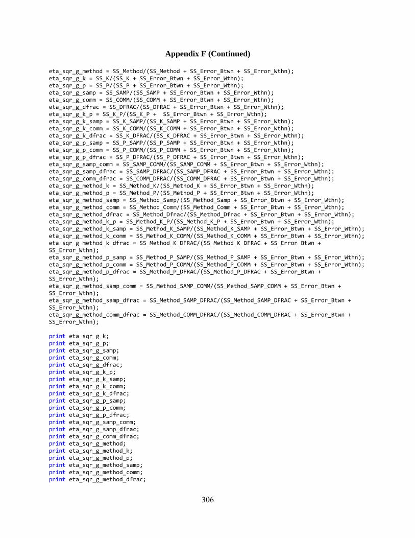
Appendix F (Continued)
306
eta_sqr_g_method = SS_Method/(SS_Method + SS_Error_Btwn + SS_Error_Wthn); eta_sqr_g_k = SS_K/(SS_K + SS_Error_Btwn + SS_Error_Wthn); eta_sqr_g_p = SS_P/(SS_P + SS_Error_Btwn + SS_Error_Wthn); eta_sqr_g_samp = SS_SAMP/(SS_SAMP + SS_Error_Btwn + SS_Error_Wthn); eta_sqr_g_comm = SS_COMM/(SS_COMM + SS_Error_Btwn + SS_Error_Wthn); eta_sqr_g_dfrac = SS_DFRAC/(SS_DFRAC + SS_Error_Btwn + SS_Error_Wthn); eta_sqr_g_k_p = SS_K_P/(SS_K_P + SS_Error_Btwn + SS_Error_Wthn); eta_sqr_g_k_samp = SS_K_SAMP/(SS_K_SAMP + SS_Error_Btwn + SS_Error_Wthn); eta_sqr_g_k_comm = SS_K_COMM/(SS_K_COMM + SS_Error_Btwn + SS_Error_Wthn); eta_sqr_g_k_dfrac = SS_K_DFRAC/(SS_K_DFRAC + SS_Error_Btwn + SS_Error_Wthn); eta_sqr_g_p_samp = SS_P_SAMP/(SS_P_SAMP + SS_Error_Btwn + SS_Error_Wthn); eta_sqr_g_p_comm = SS_P_COMM/(SS_P_COMM + SS_Error_Btwn + SS_Error_Wthn); eta_sqr_g_p_dfrac = SS_P_DFRAC/(SS_P_DFRAC + SS_Error_Btwn + SS_Error_Wthn); eta_sqr_g_samp_comm = SS_SAMP_COMM/(SS_SAMP_COMM + SS_Error_Btwn + SS_Error_Wthn); eta_sqr_g_samp_dfrac = SS_SAMP_DFRAC/(SS_SAMP_DFRAC + SS_Error_Btwn + SS_Error_Wthn); eta_sqr_g_comm_dfrac = SS_COMM_DFRAC/(SS_COMM_DFRAC + SS_Error_Btwn + SS_Error_Wthn); eta_sqr_g_method_k = SS_Method_K/(SS_Method_K + SS_Error_Btwn + SS_Error_Wthn); eta_sqr_g_method_p = SS_Method_P/(SS_Method_P + SS_Error_Btwn + SS_Error_Wthn); eta_sqr_g_method_samp = SS_Method_Samp/(SS_Method_Samp + SS_Error_Btwn + SS_Error_Wthn); eta_sqr_g_method_comm = SS_Method_Comm/(SS_Method_Comm + SS_Error_Btwn + SS_Error_Wthn); eta_sqr_g_method_dfrac = SS_Method_Dfrac/(SS_Method_Dfrac + SS_Error_Btwn + SS_Error_Wthn); eta_sqr_g_method_k_p = SS_Method_K_P/(SS_Method_K_P + SS_Error_Btwn + SS_Error_Wthn); eta_sqr_g_method_k_samp = SS_Method_K_SAMP/(SS_Method_K_SAMP + SS_Error_Btwn + SS_Error_Wthn); eta_sqr_g_method_k_comm = SS_Method_K_COMM/(SS_Method_K_COMM + SS_Error_Btwn + SS_Error_Wthn); eta_sqr_g_method_k_dfrac = SS_Method_K_DFRAC/(SS_Method_K_DFRAC + SS_Error_Btwn + SS_Error_Wthn); eta_sqr_g_method_p_samp = SS_Method_P_SAMP/(SS_Method_P_SAMP + SS_Error_Btwn + SS_Error_Wthn); eta_sqr_g_method_p_comm = SS_Method_P_COMM/(SS_Method_P_COMM + SS_Error_Btwn + SS_Error_Wthn); eta_sqr_g_method_p_dfrac = SS_Method_P_DFRAC/(SS_Method_P_DFRAC + SS_Error_Btwn + SS_Error_Wthn); eta_sqr_g_method_samp_comm = SS_Method_SAMP_COMM/(SS_Method_SAMP_COMM + SS_Error_Btwn + SS_Error_Wthn); eta_sqr_g_method_samp_dfrac = SS_Method_SAMP_DFRAC/(SS_Method_SAMP_DFRAC + SS_Error_Btwn + SS_Error_Wthn); eta_sqr_g_method_comm_dfrac = SS_Method_COMM_DFRAC/(SS_Method_COMM_DFRAC + SS_Error_Btwn + SS_Error_Wthn); print eta_sqr_g_k; print eta_sqr_g_p; print eta_sqr_g_samp; print eta_sqr_g_comm; print eta_sqr_g_dfrac; print eta_sqr_g_k_p; print eta_sqr_g_k_samp; print eta_sqr_g_k_comm; print eta_sqr_g_k_dfrac; print eta_sqr_g_p_samp; print eta_sqr_g_p_comm; print eta_sqr_g_p_dfrac; print eta_sqr_g_samp_comm; print eta_sqr_g_samp_dfrac; print eta_sqr_g_comm_dfrac; print eta_sqr_g_method; print eta_sqr_g_method_k; print eta_sqr_g_method_p; print eta_sqr_g_method_samp; print eta_sqr_g_method_comm; print eta_sqr_g_method_dfrac;
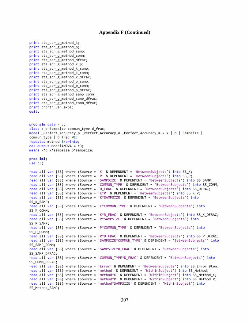
Appendix F (Continued)
307
print eta_sqr_g_method_k; print eta_sqr_g_method_p; print eta_sqr_g_method_samp; print eta_sqr_g_method_comm; print eta_sqr_g_method_dfrac; print eta_sqr_g_method_k_p; print eta_sqr_g_method_k_samp; print eta_sqr_g_method_k_comm; print eta_sqr_g_method_k_dfrac; print eta_sqr_g_method_p_samp; print eta_sqr_g_method_p_comm; print eta_sqr_g_method_p_dfrac; print eta_sqr_g_method_samp_comm; print eta_sqr_g_method_samp_dfrac; print eta_sqr_g_method_comm_dfrac; print prprtn_var_expl; quit; proc glm data = c; class k p Sampsize commun_type d_frac; model _Perfect_Accuracy_p _Perfect_Accuracy_o _Perfect_Accuracy_m = k | p | Sampsize | commun_type | d_frac @2; repeated method 3/printe; ods output ModelANOVA = c3; means k*p k*sampsize p*sampsize; proc iml; use c3; read all var {SS} where (Source = 'K' & DEPENDENT = 'BetweenSubjects') into SS_K; read all var {SS} where (Source = 'P' & DEPENDENT = 'BetweenSubjects') into SS_P; read all var {SS} where (Source = 'SAMPSIZE' & DEPENDENT = 'BetweenSubjects') into SS_SAMP; read all var {SS} where (Source = 'COMMUN_TYPE' & DEPENDENT = 'BetweenSubjects') into SS_COMM; read all var {SS} where (Source = 'D_FRAC' & DEPENDENT = 'BetweenSubjects') into SS_DFRAC; read all var {SS} where (Source = 'K*P' & DEPENDENT = 'BetweenSubjects') into SS_K_P; read all var {SS} where (Source = 'K*SAMPSIZE' & DEPENDENT = 'BetweenSubjects') into SS_K_SAMP; read all var {SS} where (Source = 'K*COMMUN_TYPE' & DEPENDENT = 'BetweenSubjects') into SS_K_COMM; read all var {SS} where (Source = 'K*D_FRAC' & DEPENDENT = 'BetweenSubjects') into SS_K_DFRAC; read all var {SS} where (Source = 'P*SAMPSIZE' & DEPENDENT = 'BetweenSubjects') into SS_P_SAMP; read all var {SS} where (Source = 'P*COMMUN_TYPE' & DEPENDENT = 'BetweenSubjects') into SS_P_COMM; read all var {SS} where (Source = 'P*D_FRAC' & DEPENDENT = 'BetweenSubjects') into SS_P_DFRAC; read all var {SS} where (Source = 'SAMPSIZE*COMMUN_TYPE' & DEPENDENT = 'BetweenSubjects') into SS_SAMP_COMM; read all var {SS} where (Source = 'SAMPSIZE*D_FRAC' & DEPENDENT = 'BetweenSubjects') into SS_SAMP_DFRAC; read all var {SS} where (Source = 'COMMUN_TYPE*D_FRAC' & DEPENDENT = 'BetweenSubjects') into SS_COMM_DFRAC; read all var {SS} where (Source = 'Error' & DEPENDENT = 'BetweenSubjects') into SS_Error_Btwn; read all var {SS} where (Source = 'method' & DEPENDENT = 'WithinSubject') into SS_Method; read all var {SS} where (Source = 'method*K' & DEPENDENT = 'WithinSubject') into SS_Method_K; read all var {SS} where (Source = 'method*P' & DEPENDENT = 'WithinSubject') into SS_Method_P; read all var {SS} where (Source = 'method*SAMPSIZE' & DEPENDENT = 'WithinSubject') into SS_Method_SAMP;
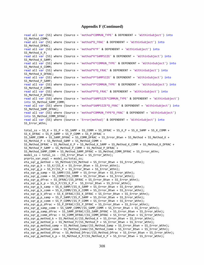
Appendix F (Continued)
308
read all var {SS} where (Source = 'method*COMMUN_TYPE' & DEPENDENT = 'WithinSubject') into SS_Method_COMM; read all var {SS} where (Source = 'method*D_FRAC' & DEPENDENT = 'WithinSubject') into SS_Method_DFRAC; read all var {SS} where (Source = 'method*K*P' & DEPENDENT = 'WithinSubject') into SS_Method_K_P; read all var {SS} where (Source = 'method*K*SAMPSIZE' & DEPENDENT = 'WithinSubject') into SS_Method_K_SAMP; read all var {SS} where (Source = 'method*K*COMMUN_TYPE' & DEPENDENT = 'WithinSubject') into SS_Method_K_COMM; read all var {SS} where (Source = 'method*K*D_FRAC' & DEPENDENT = 'WithinSubject') into SS_Method_K_DFRAC; read all var {SS} where (Source = 'method*P*SAMPSIZE' & DEPENDENT = 'WithinSubject') into SS_Method_P_SAMP; read all var {SS} where (Source = 'method*P*COMMUN_TYPE' & DEPENDENT = 'WithinSubject') into SS_Method_P_COMM; read all var {SS} where (Source = 'method*P*D_FRAC' & DEPENDENT = 'WithinSubject') into SS_Method_P_DFRAC; read all var {SS} where (Source = 'method*SAMPSIZE*COMMUN_TYPE' & DEPENDENT = 'WithinSubject') into SS_Method_SAMP_COMM; read all var {SS} where (Source = 'method*SAMPSIZE*D_FRAC' & DEPENDENT = 'WithinSubject') into SS_Method_SAMP_DFRAC; read all var {SS} where (Source = 'method*COMMUN_TYPE*D_FRAC' & DEPENDENT = 'WithinSubject') into SS_Method_COMM_DFRAC; read all var {SS} where (Source = 'Error(method)' & DEPENDENT = 'WithinSubject') into SS_Error_Wthn; total_ss = SS_K + SS_P + SS_SAMP + SS_COMM + SS_DFRAC + SS_K_P + SS_K_SAMP + SS_K_COMM + SS_K_DFRAC + SS_P_SAMP + SS_P_COMM + SS_P_DFRAC + SS_SAMP_COMM + SS_SAMP_DFRAC + SS_COMM_DFRAC + SS_Error_Btwn + SS_Method + SS_Method_K + SS_Method_P + SS_Method_SAMP + SS_Method_COMM + SS_Method_DFRAC + SS_Method_K_P + SS_Method_K_SAMP + SS_Method_K_COMM + SS_Method_K_DFRAC + SS_Method_P_SAMP + SS_Method_P_COMM + SS_Method_P_DFRAC + SS_Method_SAMP_COMM + SS_Method_SAMP_DFRAC + SS_Method_COMM_DFRAC + SS_Error_Wthn; model_ss = total_ss ‐ (SS_Error_Btwn + SS_Error_Wthn); prprtn_var_expl = model_ss/total_ss; eta_sqr_g_method = SS_Method/(SS_Method + SS_Error_Btwn + SS_Error_Wthn); eta_sqr_g_k = SS_K/(SS_K + SS_Error_Btwn + SS_Error_Wthn); eta_sqr_g_p = SS_P/(SS_P + SS_Error_Btwn + SS_Error_Wthn); eta_sqr_g_samp = SS_SAMP/(SS_SAMP + SS_Error_Btwn + SS_Error_Wthn); eta_sqr_g_comm = SS_COMM/(SS_COMM + SS_Error_Btwn + SS_Error_Wthn); eta_sqr_g_dfrac = SS_DFRAC/(SS_DFRAC + SS_Error_Btwn + SS_Error_Wthn); eta_sqr_g_k_p = SS_K_P/(SS_K_P + SS_Error_Btwn + SS_Error_Wthn); eta_sqr_g_k_samp = SS_K_SAMP/(SS_K_SAMP + SS_Error_Btwn + SS_Error_Wthn); eta_sqr_g_k_comm = SS_K_COMM/(SS_K_COMM + SS_Error_Btwn + SS_Error_Wthn); eta_sqr_g_k_dfrac = SS_K_DFRAC/(SS_K_DFRAC + SS_Error_Btwn + SS_Error_Wthn); eta_sqr_g_p_samp = SS_P_SAMP/(SS_P_SAMP + SS_Error_Btwn + SS_Error_Wthn); eta_sqr_g_p_comm = SS_P_COMM/(SS_P_COMM + SS_Error_Btwn + SS_Error_Wthn); eta_sqr_g_p_dfrac = SS_P_DFRAC/(SS_P_DFRAC + SS_Error_Btwn + SS_Error_Wthn); eta_sqr_g_samp_comm = SS_SAMP_COMM/(SS_SAMP_COMM + SS_Error_Btwn + SS_Error_Wthn); eta_sqr_g_samp_dfrac = SS_SAMP_DFRAC/(SS_SAMP_DFRAC + SS_Error_Btwn + SS_Error_Wthn); eta_sqr_g_comm_dfrac = SS_COMM_DFRAC/(SS_COMM_DFRAC + SS_Error_Btwn + SS_Error_Wthn); eta_sqr_g_method_k = SS_Method_K/(SS_Method_K + SS_Error_Btwn + SS_Error_Wthn); eta_sqr_g_method_p = SS_Method_P/(SS_Method_P + SS_Error_Btwn + SS_Error_Wthn); eta_sqr_g_method_samp = SS_Method_Samp/(SS_Method_Samp + SS_Error_Btwn + SS_Error_Wthn); eta_sqr_g_method_comm = SS_Method_Comm/(SS_Method_Comm + SS_Error_Btwn + SS_Error_Wthn); eta_sqr_g_method_dfrac = SS_Method_Dfrac/(SS_Method_Dfrac + SS_Error_Btwn + SS_Error_Wthn); eta_sqr_g_method_k_p = SS_Method_K_P/(SS_Method_K_P + SS_Error_Btwn + SS_Error_Wthn);
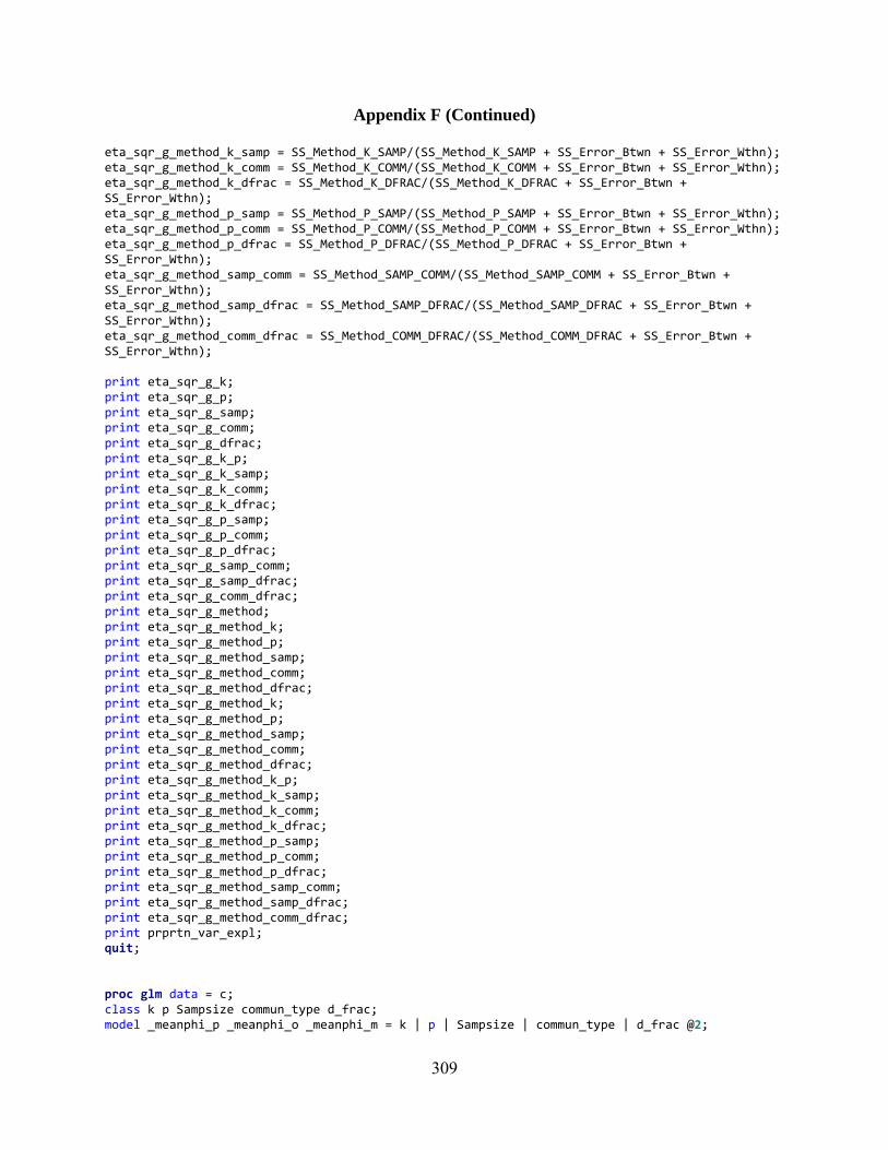
Appendix F (Continued)
309
eta_sqr_g_method_k_samp = SS_Method_K_SAMP/(SS_Method_K_SAMP + SS_Error_Btwn + SS_Error_Wthn); eta_sqr_g_method_k_comm = SS_Method_K_COMM/(SS_Method_K_COMM + SS_Error_Btwn + SS_Error_Wthn); eta_sqr_g_method_k_dfrac = SS_Method_K_DFRAC/(SS_Method_K_DFRAC + SS_Error_Btwn + SS_Error_Wthn); eta_sqr_g_method_p_samp = SS_Method_P_SAMP/(SS_Method_P_SAMP + SS_Error_Btwn + SS_Error_Wthn); eta_sqr_g_method_p_comm = SS_Method_P_COMM/(SS_Method_P_COMM + SS_Error_Btwn + SS_Error_Wthn); eta_sqr_g_method_p_dfrac = SS_Method_P_DFRAC/(SS_Method_P_DFRAC + SS_Error_Btwn + SS_Error_Wthn); eta_sqr_g_method_samp_comm = SS_Method_SAMP_COMM/(SS_Method_SAMP_COMM + SS_Error_Btwn + SS_Error_Wthn); eta_sqr_g_method_samp_dfrac = SS_Method_SAMP_DFRAC/(SS_Method_SAMP_DFRAC + SS_Error_Btwn + SS_Error_Wthn); eta_sqr_g_method_comm_dfrac = SS_Method_COMM_DFRAC/(SS_Method_COMM_DFRAC + SS_Error_Btwn + SS_Error_Wthn); print eta_sqr_g_k; print eta_sqr_g_p; print eta_sqr_g_samp; print eta_sqr_g_comm; print eta_sqr_g_dfrac; print eta_sqr_g_k_p; print eta_sqr_g_k_samp; print eta_sqr_g_k_comm; print eta_sqr_g_k_dfrac; print eta_sqr_g_p_samp; print eta_sqr_g_p_comm; print eta_sqr_g_p_dfrac; print eta_sqr_g_samp_comm; print eta_sqr_g_samp_dfrac; print eta_sqr_g_comm_dfrac; print eta_sqr_g_method; print eta_sqr_g_method_k; print eta_sqr_g_method_p; print eta_sqr_g_method_samp; print eta_sqr_g_method_comm; print eta_sqr_g_method_dfrac; print eta_sqr_g_method_k; print eta_sqr_g_method_p; print eta_sqr_g_method_samp; print eta_sqr_g_method_comm; print eta_sqr_g_method_dfrac; print eta_sqr_g_method_k_p; print eta_sqr_g_method_k_samp; print eta_sqr_g_method_k_comm; print eta_sqr_g_method_k_dfrac; print eta_sqr_g_method_p_samp; print eta_sqr_g_method_p_comm; print eta_sqr_g_method_p_dfrac; print eta_sqr_g_method_samp_comm; print eta_sqr_g_method_samp_dfrac; print eta_sqr_g_method_comm_dfrac; print prprtn_var_expl; quit; proc glm data = c; class k p Sampsize commun_type d_frac; model _meanphi_p _meanphi_o _meanphi_m = k | p | Sampsize | commun_type | d_frac @2;
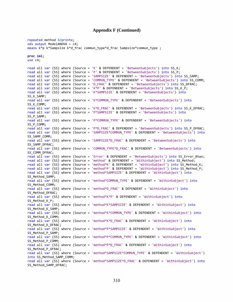
Appendix F (Continued)
310
repeated method 3/printe; ods output ModelANOVA = c4; means k*p k*Sampsize k*d_frac commun_type*d_frac Sampsize*commun_type ; proc iml; use c4; read all var {SS} where (Source = 'K' & DEPENDENT = 'BetweenSubjects') into SS_K; read all var {SS} where (Source = 'P' & DEPENDENT = 'BetweenSubjects') into SS_P; read all var {SS} where (Source = 'SAMPSIZE' & DEPENDENT = 'BetweenSubjects') into SS_SAMP; read all var {SS} where (Source = 'COMMUN_TYPE' & DEPENDENT = 'BetweenSubjects') into SS_COMM; read all var {SS} where (Source = 'D_FRAC' & DEPENDENT = 'BetweenSubjects') into SS_DFRAC; read all var {SS} where (Source = 'K*P' & DEPENDENT = 'BetweenSubjects') into SS_K_P; read all var {SS} where (Source = 'K*SAMPSIZE' & DEPENDENT = 'BetweenSubjects') into SS_K_SAMP; read all var {SS} where (Source = 'K*COMMUN_TYPE' & DEPENDENT = 'BetweenSubjects') into SS_K_COMM; read all var {SS} where (Source = 'K*D_FRAC' & DEPENDENT = 'BetweenSubjects') into SS_K_DFRAC; read all var {SS} where (Source = 'P*SAMPSIZE' & DEPENDENT = 'BetweenSubjects') into SS_P_SAMP; read all var {SS} where (Source = 'P*COMMUN_TYPE' & DEPENDENT = 'BetweenSubjects') into SS_P_COMM; read all var {SS} where (Source = 'P*D_FRAC' & DEPENDENT = 'BetweenSubjects') into SS_P_DFRAC; read all var {SS} where (Source = 'SAMPSIZE*COMMUN_TYPE' & DEPENDENT = 'BetweenSubjects') into SS_SAMP_COMM; read all var {SS} where (Source = 'SAMPSIZE*D_FRAC' & DEPENDENT = 'BetweenSubjects') into SS_SAMP_DFRAC; read all var {SS} where (Source = 'COMMUN_TYPE*D_FRAC' & DEPENDENT = 'BetweenSubjects') into SS_COMM_DFRAC; read all var {SS} where (Source = 'Error' & DEPENDENT = 'BetweenSubjects') into SS_Error_Btwn; read all var {SS} where (Source = 'method' & DEPENDENT = 'WithinSubject') into SS_Method; read all var {SS} where (Source = 'method*K' & DEPENDENT = 'WithinSubject') into SS_Method_K; read all var {SS} where (Source = 'method*P' & DEPENDENT = 'WithinSubject') into SS_Method_P; read all var {SS} where (Source = 'method*SAMPSIZE' & DEPENDENT = 'WithinSubject') into SS_Method_SAMP; read all var {SS} where (Source = 'method*COMMUN_TYPE' & DEPENDENT = 'WithinSubject') into SS_Method_COMM; read all var {SS} where (Source = 'method*D_FRAC' & DEPENDENT = 'WithinSubject') into SS_Method_DFRAC; read all var {SS} where (Source = 'method*K*P' & DEPENDENT = 'WithinSubject') into SS_Method_K_P; read all var {SS} where (Source = 'method*K*SAMPSIZE' & DEPENDENT = 'WithinSubject') into SS_Method_K_SAMP; read all var {SS} where (Source = 'method*K*COMMUN_TYPE' & DEPENDENT = 'WithinSubject') into SS_Method_K_COMM; read all var {SS} where (Source = 'method*K*D_FRAC' & DEPENDENT = 'WithinSubject') into SS_Method_K_DFRAC; read all var {SS} where (Source = 'method*P*SAMPSIZE' & DEPENDENT = 'WithinSubject') into SS_Method_P_SAMP; read all var {SS} where (Source = 'method*P*COMMUN_TYPE' & DEPENDENT = 'WithinSubject') into SS_Method_P_COMM; read all var {SS} where (Source = 'method*P*D_FRAC' & DEPENDENT = 'WithinSubject') into SS_Method_P_DFRAC; read all var {SS} where (Source = 'method*SAMPSIZE*COMMUN_TYPE' & DEPENDENT = 'WithinSubject') into SS_Method_SAMP_COMM; read all var {SS} where (Source = 'method*SAMPSIZE*D_FRAC' & DEPENDENT = 'WithinSubject') into SS_Method_SAMP_DFRAC;
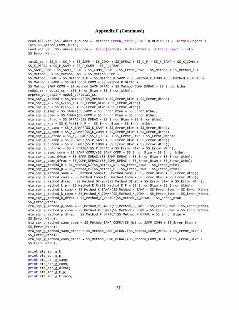
Appendix F (Continued)
311
read all var {SS} where (Source = 'method*COMMUN_TYPE*D_FRAC' & DEPENDENT = 'WithinSubject') into SS_Method_COMM_DFRAC; read all var {SS} where (Source = 'Error(method)' & DEPENDENT = 'WithinSubject') into SS_Error_Wthn; total_ss = SS_K + SS_P + SS_SAMP + SS_COMM + SS_DFRAC + SS_K_P + SS_K_SAMP + SS_K_COMM + SS_K_DFRAC + SS_P_SAMP + SS_P_COMM + SS_P_DFRAC + SS_SAMP_COMM + SS_SAMP_DFRAC + SS_COMM_DFRAC + SS_Error_Btwn + SS_Method + SS_Method_K + SS_Method_P + SS_Method_SAMP + SS_Method_COMM + SS_Method_DFRAC + SS_Method_K_P + SS_Method_K_SAMP + SS_Method_K_COMM + SS_Method_K_DFRAC + SS_Method_P_SAMP + SS_Method_P_COMM + SS_Method_P_DFRAC + SS_Method_SAMP_COMM + SS_Method_SAMP_DFRAC + SS_Method_COMM_DFRAC + SS_Error_Wthn; model_ss = total_ss ‐ (SS_Error_Btwn + SS_Error_Wthn); prprtn_var_expl = model_ss/total_ss; eta_sqr_g_method = SS_Method/(SS_Method + SS_Error_Btwn + SS_Error_Wthn); eta_sqr_g_k = SS_K/(SS_K + SS_Error_Btwn + SS_Error_Wthn); eta_sqr_g_p = SS_P/(SS_P + SS_Error_Btwn + SS_Error_Wthn); eta_sqr_g_samp = SS_SAMP/(SS_SAMP + SS_Error_Btwn + SS_Error_Wthn); eta_sqr_g_comm = SS_COMM/(SS_COMM + SS_Error_Btwn + SS_Error_Wthn); eta_sqr_g_dfrac = SS_DFRAC/(SS_DFRAC + SS_Error_Btwn + SS_Error_Wthn); eta_sqr_g_k_p = SS_K_P/(SS_K_P + SS_Error_Btwn + SS_Error_Wthn); eta_sqr_g_k_samp = SS_K_SAMP/(SS_K_SAMP + SS_Error_Btwn + SS_Error_Wthn); eta_sqr_g_k_comm = SS_K_COMM/(SS_K_COMM + SS_Error_Btwn + SS_Error_Wthn); eta_sqr_g_k_dfrac = SS_K_DFRAC/(SS_K_DFRAC + SS_Error_Btwn + SS_Error_Wthn); eta_sqr_g_p_samp = SS_P_SAMP/(SS_P_SAMP + SS_Error_Btwn + SS_Error_Wthn); eta_sqr_g_p_comm = SS_P_COMM/(SS_P_COMM + SS_Error_Btwn + SS_Error_Wthn); eta_sqr_g_p_dfrac = SS_P_DFRAC/(SS_P_DFRAC + SS_Error_Btwn + SS_Error_Wthn); eta_sqr_g_samp_comm = SS_SAMP_COMM/(SS_SAMP_COMM + SS_Error_Btwn + SS_Error_Wthn); eta_sqr_g_samp_dfrac = SS_SAMP_DFRAC/(SS_SAMP_DFRAC + SS_Error_Btwn + SS_Error_Wthn); eta_sqr_g_comm_dfrac = SS_COMM_DFRAC/(SS_COMM_DFRAC + SS_Error_Btwn + SS_Error_Wthn); eta_sqr_g_method_k = SS_Method_K/(SS_Method_K + SS_Error_Btwn + SS_Error_Wthn); eta_sqr_g_method_p = SS_Method_P/(SS_Method_P + SS_Error_Btwn + SS_Error_Wthn); eta_sqr_g_method_samp = SS_Method_Samp/(SS_Method_Samp + SS_Error_Btwn + SS_Error_Wthn); eta_sqr_g_method_comm = SS_Method_Comm/(SS_Method_Comm + SS_Error_Btwn + SS_Error_Wthn); eta_sqr_g_method_dfrac = SS_Method_Dfrac/(SS_Method_Dfrac + SS_Error_Btwn + SS_Error_Wthn); eta_sqr_g_method_k_p = SS_Method_K_P/(SS_Method_K_P + SS_Error_Btwn + SS_Error_Wthn); eta_sqr_g_method_k_samp = SS_Method_K_SAMP/(SS_Method_K_SAMP + SS_Error_Btwn + SS_Error_Wthn); eta_sqr_g_method_k_comm = SS_Method_K_COMM/(SS_Method_K_COMM + SS_Error_Btwn + SS_Error_Wthn); eta_sqr_g_method_k_dfrac = SS_Method_K_DFRAC/(SS_Method_K_DFRAC + SS_Error_Btwn + SS_Error_Wthn); eta_sqr_g_method_p_samp = SS_Method_P_SAMP/(SS_Method_P_SAMP + SS_Error_Btwn + SS_Error_Wthn); eta_sqr_g_method_p_comm = SS_Method_P_COMM/(SS_Method_P_COMM + SS_Error_Btwn + SS_Error_Wthn); eta_sqr_g_method_p_dfrac = SS_Method_P_DFRAC/(SS_Method_P_DFRAC + SS_Error_Btwn + SS_Error_Wthn); eta_sqr_g_method_samp_comm = SS_Method_SAMP_COMM/(SS_Method_SAMP_COMM + SS_Error_Btwn + SS_Error_Wthn); eta_sqr_g_method_samp_dfrac = SS_Method_SAMP_DFRAC/(SS_Method_SAMP_DFRAC + SS_Error_Btwn + SS_Error_Wthn); eta_sqr_g_method_comm_dfrac = SS_Method_COMM_DFRAC/(SS_Method_COMM_DFRAC + SS_Error_Btwn + SS_Error_Wthn); print eta_sqr_g_k; print eta_sqr_g_p; print eta_sqr_g_samp; print eta_sqr_g_comm; print eta_sqr_g_dfrac; print eta_sqr_g_k_p; print eta_sqr_g_k_samp;
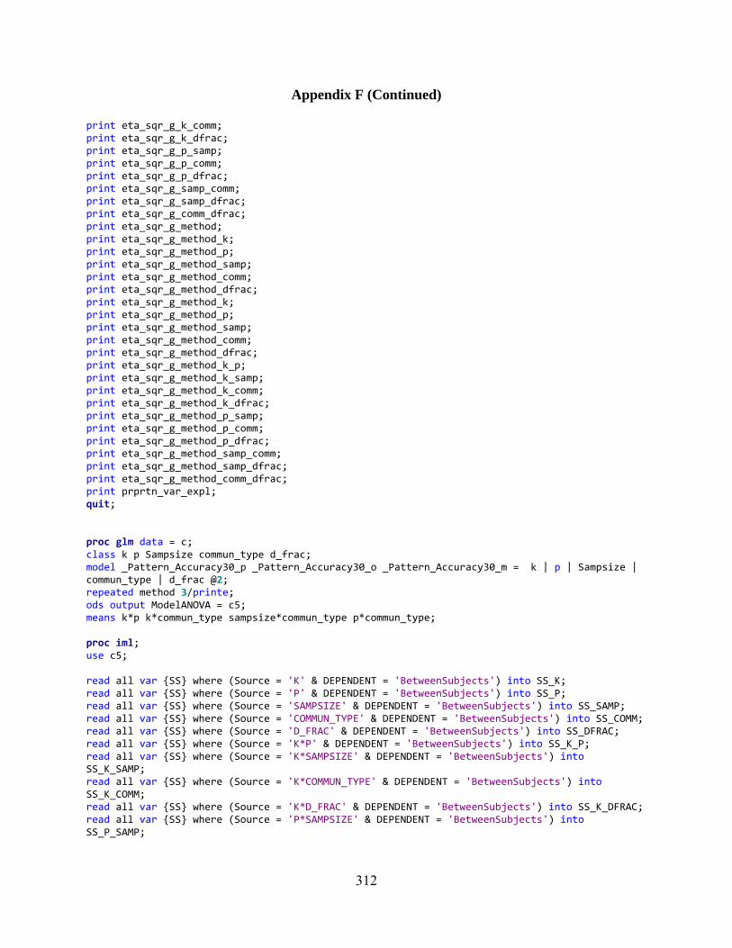
Appendix F (Continued)
312
print eta_sqr_g_k_comm; print eta_sqr_g_k_dfrac; print eta_sqr_g_p_samp; print eta_sqr_g_p_comm; print eta_sqr_g_p_dfrac; print eta_sqr_g_samp_comm; print eta_sqr_g_samp_dfrac; print eta_sqr_g_comm_dfrac; print eta_sqr_g_method; print eta_sqr_g_method_k; print eta_sqr_g_method_p; print eta_sqr_g_method_samp; print eta_sqr_g_method_comm; print eta_sqr_g_method_dfrac; print eta_sqr_g_method_k; print eta_sqr_g_method_p; print eta_sqr_g_method_samp; print eta_sqr_g_method_comm; print eta_sqr_g_method_dfrac; print eta_sqr_g_method_k_p; print eta_sqr_g_method_k_samp; print eta_sqr_g_method_k_comm; print eta_sqr_g_method_k_dfrac; print eta_sqr_g_method_p_samp; print eta_sqr_g_method_p_comm; print eta_sqr_g_method_p_dfrac; print eta_sqr_g_method_samp_comm; print eta_sqr_g_method_samp_dfrac; print eta_sqr_g_method_comm_dfrac; print prprtn_var_expl; quit; proc glm data = c; class k p Sampsize commun_type d_frac; model _Pattern_Accuracy30_p _Pattern_Accuracy30_o _Pattern_Accuracy30_m = k | p | Sampsize | commun_type | d_frac @2; repeated method 3/printe; ods output ModelANOVA = c5; means k*p k*commun_type sampsize*commun_type p*commun_type; proc iml; use c5; read all var {SS} where (Source = 'K' & DEPENDENT = 'BetweenSubjects') into SS_K; read all var {SS} where (Source = 'P' & DEPENDENT = 'BetweenSubjects') into SS_P; read all var {SS} where (Source = 'SAMPSIZE' & DEPENDENT = 'BetweenSubjects') into SS_SAMP; read all var {SS} where (Source = 'COMMUN_TYPE' & DEPENDENT = 'BetweenSubjects') into SS_COMM; read all var {SS} where (Source = 'D_FRAC' & DEPENDENT = 'BetweenSubjects') into SS_DFRAC; read all var {SS} where (Source = 'K*P' & DEPENDENT = 'BetweenSubjects') into SS_K_P; read all var {SS} where (Source = 'K*SAMPSIZE' & DEPENDENT = 'BetweenSubjects') into SS_K_SAMP; read all var {SS} where (Source = 'K*COMMUN_TYPE' & DEPENDENT = 'BetweenSubjects') into SS_K_COMM; read all var {SS} where (Source = 'K*D_FRAC' & DEPENDENT = 'BetweenSubjects') into SS_K_DFRAC; read all var {SS} where (Source = 'P*SAMPSIZE' & DEPENDENT = 'BetweenSubjects') into SS_P_SAMP;

Appendix F (Continued)
313
read all var {SS} where (Source = 'P*COMMUN_TYPE' & DEPENDENT = 'BetweenSubjects') into SS_P_COMM; read all var {SS} where (Source = 'P*D_FRAC' & DEPENDENT = 'BetweenSubjects') into SS_P_DFRAC; read all var {SS} where (Source = 'SAMPSIZE*COMMUN_TYPE' & DEPENDENT = 'BetweenSubjects') into SS_SAMP_COMM; read all var {SS} where (Source = 'SAMPSIZE*D_FRAC' & DEPENDENT = 'BetweenSubjects') into SS_SAMP_DFRAC; read all var {SS} where (Source = 'COMMUN_TYPE*D_FRAC' & DEPENDENT = 'BetweenSubjects') into SS_COMM_DFRAC; read all var {SS} where (Source = 'Error' & DEPENDENT = 'BetweenSubjects') into SS_Error_Btwn; read all var {SS} where (Source = 'method' & DEPENDENT = 'WithinSubject') into SS_Method; read all var {SS} where (Source = 'method*K' & DEPENDENT = 'WithinSubject') into SS_Method_K; read all var {SS} where (Source = 'method*P' & DEPENDENT = 'WithinSubject') into SS_Method_P; read all var {SS} where (Source = 'method*SAMPSIZE' & DEPENDENT = 'WithinSubject') into SS_Method_SAMP; read all var {SS} where (Source = 'method*COMMUN_TYPE' & DEPENDENT = 'WithinSubject') into SS_Method_COMM; read all var {SS} where (Source = 'method*D_FRAC' & DEPENDENT = 'WithinSubject') into SS_Method_DFRAC; read all var {SS} where (Source = 'method*K*P' & DEPENDENT = 'WithinSubject') into SS_Method_K_P; read all var {SS} where (Source = 'method*K*SAMPSIZE' & DEPENDENT = 'WithinSubject') into SS_Method_K_SAMP; read all var {SS} where (Source = 'method*K*COMMUN_TYPE' & DEPENDENT = 'WithinSubject') into SS_Method_K_COMM; read all var {SS} where (Source = 'method*K*D_FRAC' & DEPENDENT = 'WithinSubject') into SS_Method_K_DFRAC; read all var {SS} where (Source = 'method*P*SAMPSIZE' & DEPENDENT = 'WithinSubject') into SS_Method_P_SAMP; read all var {SS} where (Source = 'method*P*COMMUN_TYPE' & DEPENDENT = 'WithinSubject') into SS_Method_P_COMM; read all var {SS} where (Source = 'method*P*D_FRAC' & DEPENDENT = 'WithinSubject') into SS_Method_P_DFRAC; read all var {SS} where (Source = 'method*SAMPSIZE*COMMUN_TYPE' & DEPENDENT = 'WithinSubject') into SS_Method_SAMP_COMM; read all var {SS} where (Source = 'method*SAMPSIZE*D_FRAC' & DEPENDENT = 'WithinSubject') into SS_Method_SAMP_DFRAC; read all var {SS} where (Source = 'method*COMMUN_TYPE*D_FRAC' & DEPENDENT = 'WithinSubject') into SS_Method_COMM_DFRAC; read all var {SS} where (Source = 'Error(method)' & DEPENDENT = 'WithinSubject') into SS_Error_Wthn; total_ss = SS_K + SS_P + SS_SAMP + SS_COMM + SS_DFRAC + SS_K_P + SS_K_SAMP + SS_K_COMM + SS_K_DFRAC + SS_P_SAMP + SS_P_COMM + SS_P_DFRAC + SS_SAMP_COMM + SS_SAMP_DFRAC + SS_COMM_DFRAC + SS_Error_Btwn + SS_Method + SS_Method_K + SS_Method_P + SS_Method_SAMP + SS_Method_COMM + SS_Method_DFRAC + SS_Method_K_P + SS_Method_K_SAMP + SS_Method_K_COMM + SS_Method_K_DFRAC + SS_Method_P_SAMP + SS_Method_P_COMM + SS_Method_P_DFRAC + SS_Method_SAMP_COMM + SS_Method_SAMP_DFRAC + SS_Method_COMM_DFRAC + SS_Error_Wthn; model_ss = total_ss ‐ (SS_Error_Btwn + SS_Error_Wthn); prprtn_var_expl = model_ss/total_ss; eta_sqr_g_method = SS_Method/(SS_Method + SS_Error_Btwn + SS_Error_Wthn); eta_sqr_g_k = SS_K/(SS_K + SS_Error_Btwn + SS_Error_Wthn); eta_sqr_g_p = SS_P/(SS_P + SS_Error_Btwn + SS_Error_Wthn); eta_sqr_g_samp = SS_SAMP/(SS_SAMP + SS_Error_Btwn + SS_Error_Wthn); eta_sqr_g_comm = SS_COMM/(SS_COMM + SS_Error_Btwn + SS_Error_Wthn); eta_sqr_g_dfrac = SS_DFRAC/(SS_DFRAC + SS_Error_Btwn + SS_Error_Wthn); eta_sqr_g_k_p = SS_K_P/(SS_K_P + SS_Error_Btwn + SS_Error_Wthn);
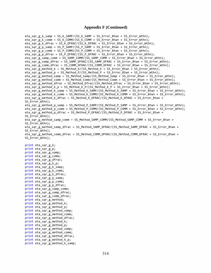
Appendix F (Continued)
314
eta_sqr_g_k_samp = SS_K_SAMP/(SS_K_SAMP + SS_Error_Btwn + SS_Error_Wthn); eta_sqr_g_k_comm = SS_K_COMM/(SS_K_COMM + SS_Error_Btwn + SS_Error_Wthn); eta_sqr_g_k_dfrac = SS_K_DFRAC/(SS_K_DFRAC + SS_Error_Btwn + SS_Error_Wthn); eta_sqr_g_p_samp = SS_P_SAMP/(SS_P_SAMP + SS_Error_Btwn + SS_Error_Wthn); eta_sqr_g_p_comm = SS_P_COMM/(SS_P_COMM + SS_Error_Btwn + SS_Error_Wthn); eta_sqr_g_p_dfrac = SS_P_DFRAC/(SS_P_DFRAC + SS_Error_Btwn + SS_Error_Wthn); eta_sqr_g_samp_comm = SS_SAMP_COMM/(SS_SAMP_COMM + SS_Error_Btwn + SS_Error_Wthn); eta_sqr_g_samp_dfrac = SS_SAMP_DFRAC/(SS_SAMP_DFRAC + SS_Error_Btwn + SS_Error_Wthn); eta_sqr_g_comm_dfrac = SS_COMM_DFRAC/(SS_COMM_DFRAC + SS_Error_Btwn + SS_Error_Wthn); eta_sqr_g_method_k = SS_Method_K/(SS_Method_K + SS_Error_Btwn + SS_Error_Wthn); eta_sqr_g_method_p = SS_Method_P/(SS_Method_P + SS_Error_Btwn + SS_Error_Wthn); eta_sqr_g_method_samp = SS_Method_Samp/(SS_Method_Samp + SS_Error_Btwn + SS_Error_Wthn); eta_sqr_g_method_comm = SS_Method_Comm/(SS_Method_Comm + SS_Error_Btwn + SS_Error_Wthn); eta_sqr_g_method_dfrac = SS_Method_Dfrac/(SS_Method_Dfrac + SS_Error_Btwn + SS_Error_Wthn); eta_sqr_g_method_k_p = SS_Method_K_P/(SS_Method_K_P + SS_Error_Btwn + SS_Error_Wthn); eta_sqr_g_method_k_samp = SS_Method_K_SAMP/(SS_Method_K_SAMP + SS_Error_Btwn + SS_Error_Wthn); eta_sqr_g_method_k_comm = SS_Method_K_COMM/(SS_Method_K_COMM + SS_Error_Btwn + SS_Error_Wthn); eta_sqr_g_method_k_dfrac = SS_Method_K_DFRAC/(SS_Method_K_DFRAC + SS_Error_Btwn + SS_Error_Wthn); eta_sqr_g_method_p_samp = SS_Method_P_SAMP/(SS_Method_P_SAMP + SS_Error_Btwn + SS_Error_Wthn); eta_sqr_g_method_p_comm = SS_Method_P_COMM/(SS_Method_P_COMM + SS_Error_Btwn + SS_Error_Wthn); eta_sqr_g_method_p_dfrac = SS_Method_P_DFRAC/(SS_Method_P_DFRAC + SS_Error_Btwn + SS_Error_Wthn); eta_sqr_g_method_samp_comm = SS_Method_SAMP_COMM/(SS_Method_SAMP_COMM + SS_Error_Btwn + SS_Error_Wthn); eta_sqr_g_method_samp_dfrac = SS_Method_SAMP_DFRAC/(SS_Method_SAMP_DFRAC + SS_Error_Btwn + SS_Error_Wthn); eta_sqr_g_method_comm_dfrac = SS_Method_COMM_DFRAC/(SS_Method_COMM_DFRAC + SS_Error_Btwn + SS_Error_Wthn); print eta_sqr_g_k; print eta_sqr_g_p; print eta_sqr_g_samp; print eta_sqr_g_comm; print eta_sqr_g_dfrac; print eta_sqr_g_k_p; print eta_sqr_g_k_samp; print eta_sqr_g_k_comm; print eta_sqr_g_k_dfrac; print eta_sqr_g_p_samp; print eta_sqr_g_p_comm; print eta_sqr_g_p_dfrac; print eta_sqr_g_samp_comm; print eta_sqr_g_samp_dfrac; print eta_sqr_g_comm_dfrac; print eta_sqr_g_method; print eta_sqr_g_method_k; print eta_sqr_g_method_p; print eta_sqr_g_method_samp; print eta_sqr_g_method_comm; print eta_sqr_g_method_dfrac; print eta_sqr_g_method_k; print eta_sqr_g_method_p; print eta_sqr_g_method_samp; print eta_sqr_g_method_comm; print eta_sqr_g_method_dfrac; print eta_sqr_g_method_k_p; print eta_sqr_g_method_k_samp;
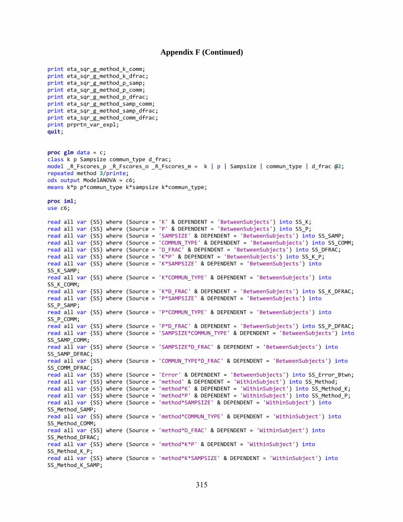
Appendix F (Continued)
315
print eta_sqr_g_method_k_comm; print eta_sqr_g_method_k_dfrac; print eta_sqr_g_method_p_samp; print eta_sqr_g_method_p_comm; print eta_sqr_g_method_p_dfrac; print eta_sqr_g_method_samp_comm; print eta_sqr_g_method_samp_dfrac; print eta_sqr_g_method_comm_dfrac; print prprtn_var_expl; quit; proc glm data = c; class k p Sampsize commun_type d_frac; model _R_Fscores_p _R_Fscores_o _R_Fscores_m = k | p | Sampsize | commun_type | d_frac @2; repeated method 3/printe; ods output ModelANOVA = c6; means k*p p*commun_type k*sampsize k*commun_type; proc iml; use c6; read all var {SS} where (Source = 'K' & DEPENDENT = 'BetweenSubjects') into SS_K; read all var {SS} where (Source = 'P' & DEPENDENT = 'BetweenSubjects') into SS_P; read all var {SS} where (Source = 'SAMPSIZE' & DEPENDENT = 'BetweenSubjects') into SS_SAMP; read all var {SS} where (Source = 'COMMUN_TYPE' & DEPENDENT = 'BetweenSubjects') into SS_COMM; read all var {SS} where (Source = 'D_FRAC' & DEPENDENT = 'BetweenSubjects') into SS_DFRAC; read all var {SS} where (Source = 'K*P' & DEPENDENT = 'BetweenSubjects') into SS_K_P; read all var {SS} where (Source = 'K*SAMPSIZE' & DEPENDENT = 'BetweenSubjects') into SS_K_SAMP; read all var {SS} where (Source = 'K*COMMUN_TYPE' & DEPENDENT = 'BetweenSubjects') into SS_K_COMM; read all var {SS} where (Source = 'K*D_FRAC' & DEPENDENT = 'BetweenSubjects') into SS_K_DFRAC; read all var {SS} where (Source = 'P*SAMPSIZE' & DEPENDENT = 'BetweenSubjects') into SS_P_SAMP; read all var {SS} where (Source = 'P*COMMUN_TYPE' & DEPENDENT = 'BetweenSubjects') into SS_P_COMM; read all var {SS} where (Source = 'P*D_FRAC' & DEPENDENT = 'BetweenSubjects') into SS_P_DFRAC; read all var {SS} where (Source = 'SAMPSIZE*COMMUN_TYPE' & DEPENDENT = 'BetweenSubjects') into SS_SAMP_COMM; read all var {SS} where (Source = 'SAMPSIZE*D_FRAC' & DEPENDENT = 'BetweenSubjects') into SS_SAMP_DFRAC; read all var {SS} where (Source = 'COMMUN_TYPE*D_FRAC' & DEPENDENT = 'BetweenSubjects') into SS_COMM_DFRAC; read all var {SS} where (Source = 'Error' & DEPENDENT = 'BetweenSubjects') into SS_Error_Btwn; read all var {SS} where (Source = 'method' & DEPENDENT = 'WithinSubject') into SS_Method; read all var {SS} where (Source = 'method*K' & DEPENDENT = 'WithinSubject') into SS_Method_K; read all var {SS} where (Source = 'method*P' & DEPENDENT = 'WithinSubject') into SS_Method_P; read all var {SS} where (Source = 'method*SAMPSIZE' & DEPENDENT = 'WithinSubject') into SS_Method_SAMP; read all var {SS} where (Source = 'method*COMMUN_TYPE' & DEPENDENT = 'WithinSubject') into SS_Method_COMM; read all var {SS} where (Source = 'method*D_FRAC' & DEPENDENT = 'WithinSubject') into SS_Method_DFRAC; read all var {SS} where (Source = 'method*K*P' & DEPENDENT = 'WithinSubject') into SS_Method_K_P; read all var {SS} where (Source = 'method*K*SAMPSIZE' & DEPENDENT = 'WithinSubject') into SS_Method_K_SAMP;

Appendix F (Continued)
316
read all var {SS} where (Source = 'method*K*COMMUN_TYPE' & DEPENDENT = 'WithinSubject') into SS_Method_K_COMM; read all var {SS} where (Source = 'method*K*D_FRAC' & DEPENDENT = 'WithinSubject') into SS_Method_K_DFRAC; read all var {SS} where (Source = 'method*P*SAMPSIZE' & DEPENDENT = 'WithinSubject') into SS_Method_P_SAMP; read all var {SS} where (Source = 'method*P*COMMUN_TYPE' & DEPENDENT = 'WithinSubject') into SS_Method_P_COMM; read all var {SS} where (Source = 'method*P*D_FRAC' & DEPENDENT = 'WithinSubject') into SS_Method_P_DFRAC; read all var {SS} where (Source = 'method*SAMPSIZE*COMMUN_TYPE' & DEPENDENT = 'WithinSubject') into SS_Method_SAMP_COMM; read all var {SS} where (Source = 'method*SAMPSIZE*D_FRAC' & DEPENDENT = 'WithinSubject') into SS_Method_SAMP_DFRAC; read all var {SS} where (Source = 'method*COMMUN_TYPE*D_FRAC' & DEPENDENT = 'WithinSubject') into SS_Method_COMM_DFRAC; read all var {SS} where (Source = 'Error(method)' & DEPENDENT = 'WithinSubject') into SS_Error_Wthn; total_ss = SS_K + SS_P + SS_SAMP + SS_COMM + SS_DFRAC + SS_K_P + SS_K_SAMP + SS_K_COMM + SS_K_DFRAC + SS_P_SAMP + SS_P_COMM + SS_P_DFRAC + SS_SAMP_COMM + SS_SAMP_DFRAC + SS_COMM_DFRAC + SS_Error_Btwn + SS_Method + SS_Method_K + SS_Method_P + SS_Method_SAMP + SS_Method_COMM + SS_Method_DFRAC + SS_Method_K_P + SS_Method_K_SAMP + SS_Method_K_COMM + SS_Method_K_DFRAC + SS_Method_P_SAMP + SS_Method_P_COMM + SS_Method_P_DFRAC + SS_Method_SAMP_COMM + SS_Method_SAMP_DFRAC + SS_Method_COMM_DFRAC + SS_Error_Wthn; model_ss = total_ss ‐ (SS_Error_Btwn + SS_Error_Wthn); prprtn_var_expl = model_ss/total_ss; eta_sqr_g_method = SS_Method/(SS_Method + SS_Error_Btwn + SS_Error_Wthn); eta_sqr_g_k = SS_K/(SS_K + SS_Error_Btwn + SS_Error_Wthn); eta_sqr_g_p = SS_P/(SS_P + SS_Error_Btwn + SS_Error_Wthn); eta_sqr_g_samp = SS_SAMP/(SS_SAMP + SS_Error_Btwn + SS_Error_Wthn); eta_sqr_g_comm = SS_COMM/(SS_COMM + SS_Error_Btwn + SS_Error_Wthn); eta_sqr_g_dfrac = SS_DFRAC/(SS_DFRAC + SS_Error_Btwn + SS_Error_Wthn); eta_sqr_g_k_p = SS_K_P/(SS_K_P + SS_Error_Btwn + SS_Error_Wthn); eta_sqr_g_k_samp = SS_K_SAMP/(SS_K_SAMP + SS_Error_Btwn + SS_Error_Wthn); eta_sqr_g_k_comm = SS_K_COMM/(SS_K_COMM + SS_Error_Btwn + SS_Error_Wthn); eta_sqr_g_k_dfrac = SS_K_DFRAC/(SS_K_DFRAC + SS_Error_Btwn + SS_Error_Wthn); eta_sqr_g_p_samp = SS_P_SAMP/(SS_P_SAMP + SS_Error_Btwn + SS_Error_Wthn); eta_sqr_g_p_comm = SS_P_COMM/(SS_P_COMM + SS_Error_Btwn + SS_Error_Wthn); eta_sqr_g_p_dfrac = SS_P_DFRAC/(SS_P_DFRAC + SS_Error_Btwn + SS_Error_Wthn); eta_sqr_g_samp_comm = SS_SAMP_COMM/(SS_SAMP_COMM + SS_Error_Btwn + SS_Error_Wthn); eta_sqr_g_samp_dfrac = SS_SAMP_DFRAC/(SS_SAMP_DFRAC + SS_Error_Btwn + SS_Error_Wthn); eta_sqr_g_comm_dfrac = SS_COMM_DFRAC/(SS_COMM_DFRAC + SS_Error_Btwn + SS_Error_Wthn); eta_sqr_g_method_k = SS_Method_K/(SS_Method_K + SS_Error_Btwn + SS_Error_Wthn); eta_sqr_g_method_p = SS_Method_P/(SS_Method_P + SS_Error_Btwn + SS_Error_Wthn); eta_sqr_g_method_samp = SS_Method_Samp/(SS_Method_Samp + SS_Error_Btwn + SS_Error_Wthn); eta_sqr_g_method_comm = SS_Method_Comm/(SS_Method_Comm + SS_Error_Btwn + SS_Error_Wthn); eta_sqr_g_method_dfrac = SS_Method_Dfrac/(SS_Method_Dfrac + SS_Error_Btwn + SS_Error_Wthn); eta_sqr_g_method_k_p = SS_Method_K_P/(SS_Method_K_P + SS_Error_Btwn + SS_Error_Wthn); eta_sqr_g_method_k_samp = SS_Method_K_SAMP/(SS_Method_K_SAMP + SS_Error_Btwn + SS_Error_Wthn); eta_sqr_g_method_k_comm = SS_Method_K_COMM/(SS_Method_K_COMM + SS_Error_Btwn + SS_Error_Wthn); eta_sqr_g_method_k_dfrac = SS_Method_K_DFRAC/(SS_Method_K_DFRAC + SS_Error_Btwn + SS_Error_Wthn); eta_sqr_g_method_p_samp = SS_Method_P_SAMP/(SS_Method_P_SAMP + SS_Error_Btwn + SS_Error_Wthn); eta_sqr_g_method_p_comm = SS_Method_P_COMM/(SS_Method_P_COMM + SS_Error_Btwn + SS_Error_Wthn); eta_sqr_g_method_p_dfrac = SS_Method_P_DFRAC/(SS_Method_P_DFRAC + SS_Error_Btwn + SS_Error_Wthn);
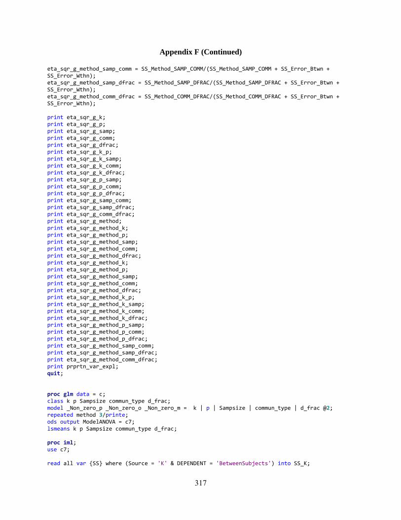
Appendix F (Continued)
317
eta_sqr_g_method_samp_comm = SS_Method_SAMP_COMM/(SS_Method_SAMP_COMM + SS_Error_Btwn + SS_Error_Wthn); eta_sqr_g_method_samp_dfrac = SS_Method_SAMP_DFRAC/(SS_Method_SAMP_DFRAC + SS_Error_Btwn + SS_Error_Wthn); eta_sqr_g_method_comm_dfrac = SS_Method_COMM_DFRAC/(SS_Method_COMM_DFRAC + SS_Error_Btwn + SS_Error_Wthn); print eta_sqr_g_k; print eta_sqr_g_p; print eta_sqr_g_samp; print eta_sqr_g_comm; print eta_sqr_g_dfrac; print eta_sqr_g_k_p; print eta_sqr_g_k_samp; print eta_sqr_g_k_comm; print eta_sqr_g_k_dfrac; print eta_sqr_g_p_samp; print eta_sqr_g_p_comm; print eta_sqr_g_p_dfrac; print eta_sqr_g_samp_comm; print eta_sqr_g_samp_dfrac; print eta_sqr_g_comm_dfrac; print eta_sqr_g_method; print eta_sqr_g_method_k; print eta_sqr_g_method_p; print eta_sqr_g_method_samp; print eta_sqr_g_method_comm; print eta_sqr_g_method_dfrac; print eta_sqr_g_method_k; print eta_sqr_g_method_p; print eta_sqr_g_method_samp; print eta_sqr_g_method_comm; print eta_sqr_g_method_dfrac; print eta_sqr_g_method_k_p; print eta_sqr_g_method_k_samp; print eta_sqr_g_method_k_comm; print eta_sqr_g_method_k_dfrac; print eta_sqr_g_method_p_samp; print eta_sqr_g_method_p_comm; print eta_sqr_g_method_p_dfrac; print eta_sqr_g_method_samp_comm; print eta_sqr_g_method_samp_dfrac; print eta_sqr_g_method_comm_dfrac; print prprtn_var_expl; quit; proc glm data = c; class k p Sampsize commun_type d_frac; model _Non_zero_p _Non_zero_o _Non_zero_m = k | p | Sampsize | commun_type | d_frac @2; repeated method 3/printe; ods output ModelANOVA = c7; lsmeans k p Sampsize commun_type d_frac; proc iml; use c7; read all var {SS} where (Source = 'K' & DEPENDENT = 'BetweenSubjects') into SS_K;

Appendix F (Continued)
318
read all var {SS} where (Source = 'P' & DEPENDENT = 'BetweenSubjects') into SS_P; read all var {SS} where (Source = 'SAMPSIZE' & DEPENDENT = 'BetweenSubjects') into SS_SAMP; read all var {SS} where (Source = 'COMMUN_TYPE' & DEPENDENT = 'BetweenSubjects') into SS_COMM; read all var {SS} where (Source = 'D_FRAC' & DEPENDENT = 'BetweenSubjects') into SS_DFRAC; read all var {SS} where (Source = 'K*P' & DEPENDENT = 'BetweenSubjects') into SS_K_P; read all var {SS} where (Source = 'K*SAMPSIZE' & DEPENDENT = 'BetweenSubjects') into SS_K_SAMP; read all var {SS} where (Source = 'K*COMMUN_TYPE' & DEPENDENT = 'BetweenSubjects') into SS_K_COMM; read all var {SS} where (Source = 'K*D_FRAC' & DEPENDENT = 'BetweenSubjects') into SS_K_DFRAC; read all var {SS} where (Source = 'P*SAMPSIZE' & DEPENDENT = 'BetweenSubjects') into SS_P_SAMP; read all var {SS} where (Source = 'P*COMMUN_TYPE' & DEPENDENT = 'BetweenSubjects') into SS_P_COMM; read all var {SS} where (Source = 'P*D_FRAC' & DEPENDENT = 'BetweenSubjects') into SS_P_DFRAC; read all var {SS} where (Source = 'SAMPSIZE*COMMUN_TYPE' & DEPENDENT = 'BetweenSubjects') into SS_SAMP_COMM; read all var {SS} where (Source = 'SAMPSIZE*D_FRAC' & DEPENDENT = 'BetweenSubjects') into SS_SAMP_DFRAC; read all var {SS} where (Source = 'COMMUN_TYPE*D_FRAC' & DEPENDENT = 'BetweenSubjects') into SS_COMM_DFRAC; read all var {SS} where (Source = 'Error' & DEPENDENT = 'BetweenSubjects') into SS_Error_Btwn; read all var {SS} where (Source = 'method' & DEPENDENT = 'WithinSubject') into SS_Method; read all var {SS} where (Source = 'method*K' & DEPENDENT = 'WithinSubject') into SS_Method_K; read all var {SS} where (Source = 'method*P' & DEPENDENT = 'WithinSubject') into SS_Method_P; read all var {SS} where (Source = 'method*SAMPSIZE' & DEPENDENT = 'WithinSubject') into SS_Method_SAMP; read all var {SS} where (Source = 'method*COMMUN_TYPE' & DEPENDENT = 'WithinSubject') into SS_Method_COMM; read all var {SS} where (Source = 'method*D_FRAC' & DEPENDENT = 'WithinSubject') into SS_Method_DFRAC; read all var {SS} where (Source = 'method*K*P' & DEPENDENT = 'WithinSubject') into SS_Method_K_P; read all var {SS} where (Source = 'method*K*SAMPSIZE' & DEPENDENT = 'WithinSubject') into SS_Method_K_SAMP; read all var {SS} where (Source = 'method*K*COMMUN_TYPE' & DEPENDENT = 'WithinSubject') into SS_Method_K_COMM; read all var {SS} where (Source = 'method*K*D_FRAC' & DEPENDENT = 'WithinSubject') into SS_Method_K_DFRAC; read all var {SS} where (Source = 'method*P*SAMPSIZE' & DEPENDENT = 'WithinSubject') into SS_Method_P_SAMP; read all var {SS} where (Source = 'method*P*COMMUN_TYPE' & DEPENDENT = 'WithinSubject') into SS_Method_P_COMM; read all var {SS} where (Source = 'method*P*D_FRAC' & DEPENDENT = 'WithinSubject') into SS_Method_P_DFRAC; read all var {SS} where (Source = 'method*SAMPSIZE*COMMUN_TYPE' & DEPENDENT = 'WithinSubject') into SS_Method_SAMP_COMM; read all var {SS} where (Source = 'method*SAMPSIZE*D_FRAC' & DEPENDENT = 'WithinSubject') into SS_Method_SAMP_DFRAC; read all var {SS} where (Source = 'method*COMMUN_TYPE*D_FRAC' & DEPENDENT = 'WithinSubject') into SS_Method_COMM_DFRAC; read all var {SS} where (Source = 'Error(method)' & DEPENDENT = 'WithinSubject') into SS_Error_Wthn; total_ss = SS_K + SS_P + SS_SAMP + SS_COMM + SS_DFRAC + SS_K_P + SS_K_SAMP + SS_K_COMM + SS_K_DFRAC + SS_P_SAMP + SS_P_COMM + SS_P_DFRAC + SS_SAMP_COMM + SS_SAMP_DFRAC + SS_COMM_DFRAC + SS_Error_Btwn + SS_Method + SS_Method_K + SS_Method_P + SS_Method_SAMP + SS_Method_COMM +

Appendix F (Continued)
319
SS_Method_DFRAC + SS_Method_K_P + SS_Method_K_SAMP + SS_Method_K_COMM + SS_Method_K_DFRAC + SS_Method_P_SAMP + SS_Method_P_COMM + SS_Method_P_DFRAC + SS_Method_SAMP_COMM + SS_Method_SAMP_DFRAC + SS_Method_COMM_DFRAC + SS_Error_Wthn; model_ss = total_ss ‐ (SS_Error_Btwn + SS_Error_Wthn); prprtn_var_expl = model_ss/total_ss; eta_sqr_g_method = SS_Method/(SS_Method + SS_Error_Btwn + SS_Error_Wthn); eta_sqr_g_k = SS_K/(SS_K + SS_Error_Btwn + SS_Error_Wthn); eta_sqr_g_p = SS_P/(SS_P + SS_Error_Btwn + SS_Error_Wthn); eta_sqr_g_samp = SS_SAMP/(SS_SAMP + SS_Error_Btwn + SS_Error_Wthn); eta_sqr_g_comm = SS_COMM/(SS_COMM + SS_Error_Btwn + SS_Error_Wthn); eta_sqr_g_dfrac = SS_DFRAC/(SS_DFRAC + SS_Error_Btwn + SS_Error_Wthn); eta_sqr_g_k_p = SS_K_P/(SS_K_P + SS_Error_Btwn + SS_Error_Wthn); eta_sqr_g_k_samp = SS_K_SAMP/(SS_K_SAMP + SS_Error_Btwn + SS_Error_Wthn); eta_sqr_g_k_comm = SS_K_COMM/(SS_K_COMM + SS_Error_Btwn + SS_Error_Wthn); eta_sqr_g_k_dfrac = SS_K_DFRAC/(SS_K_DFRAC + SS_Error_Btwn + SS_Error_Wthn); eta_sqr_g_p_samp = SS_P_SAMP/(SS_P_SAMP + SS_Error_Btwn + SS_Error_Wthn); eta_sqr_g_p_comm = SS_P_COMM/(SS_P_COMM + SS_Error_Btwn + SS_Error_Wthn); eta_sqr_g_p_dfrac = SS_P_DFRAC/(SS_P_DFRAC + SS_Error_Btwn + SS_Error_Wthn); eta_sqr_g_samp_comm = SS_SAMP_COMM/(SS_SAMP_COMM + SS_Error_Btwn + SS_Error_Wthn); eta_sqr_g_samp_dfrac = SS_SAMP_DFRAC/(SS_SAMP_DFRAC + SS_Error_Btwn + SS_Error_Wthn); eta_sqr_g_comm_dfrac = SS_COMM_DFRAC/(SS_COMM_DFRAC + SS_Error_Btwn + SS_Error_Wthn); eta_sqr_g_method_k = SS_Method_K/(SS_Method_K + SS_Error_Btwn + SS_Error_Wthn); eta_sqr_g_method_p = SS_Method_P/(SS_Method_P + SS_Error_Btwn + SS_Error_Wthn); eta_sqr_g_method_samp = SS_Method_Samp/(SS_Method_Samp + SS_Error_Btwn + SS_Error_Wthn); eta_sqr_g_method_comm = SS_Method_Comm/(SS_Method_Comm + SS_Error_Btwn + SS_Error_Wthn); eta_sqr_g_method_dfrac = SS_Method_Dfrac/(SS_Method_Dfrac + SS_Error_Btwn + SS_Error_Wthn); eta_sqr_g_method_k_p = SS_Method_K_P/(SS_Method_K_P + SS_Error_Btwn + SS_Error_Wthn); eta_sqr_g_method_k_samp = SS_Method_K_SAMP/(SS_Method_K_SAMP + SS_Error_Btwn + SS_Error_Wthn); eta_sqr_g_method_k_comm = SS_Method_K_COMM/(SS_Method_K_COMM + SS_Error_Btwn + SS_Error_Wthn); eta_sqr_g_method_k_dfrac = SS_Method_K_DFRAC/(SS_Method_K_DFRAC + SS_Error_Btwn + SS_Error_Wthn); eta_sqr_g_method_p_samp = SS_Method_P_SAMP/(SS_Method_P_SAMP + SS_Error_Btwn + SS_Error_Wthn); eta_sqr_g_method_p_comm = SS_Method_P_COMM/(SS_Method_P_COMM + SS_Error_Btwn + SS_Error_Wthn); eta_sqr_g_method_p_dfrac = SS_Method_P_DFRAC/(SS_Method_P_DFRAC + SS_Error_Btwn + SS_Error_Wthn); eta_sqr_g_method_samp_comm = SS_Method_SAMP_COMM/(SS_Method_SAMP_COMM + SS_Error_Btwn + SS_Error_Wthn); eta_sqr_g_method_samp_dfrac = SS_Method_SAMP_DFRAC/(SS_Method_SAMP_DFRAC + SS_Error_Btwn + SS_Error_Wthn); eta_sqr_g_method_comm_dfrac = SS_Method_COMM_DFRAC/(SS_Method_COMM_DFRAC + SS_Error_Btwn + SS_Error_Wthn); print eta_sqr_g_k; print eta_sqr_g_p; print eta_sqr_g_samp; print eta_sqr_g_comm; print eta_sqr_g_dfrac; print eta_sqr_g_k_p; print eta_sqr_g_k_samp; print eta_sqr_g_k_comm; print eta_sqr_g_k_dfrac; print eta_sqr_g_p_samp; print eta_sqr_g_p_comm; print eta_sqr_g_p_dfrac; print eta_sqr_g_samp_comm; print eta_sqr_g_samp_dfrac; print eta_sqr_g_comm_dfrac; print eta_sqr_g_method;
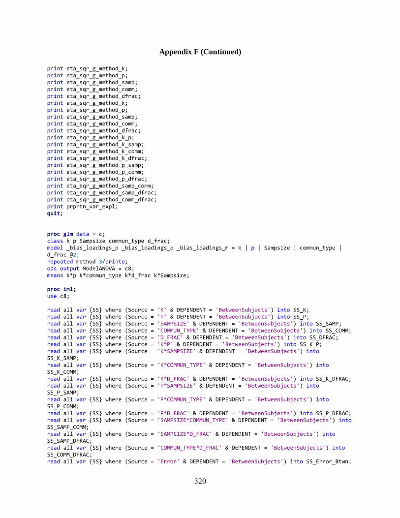
Appendix F (Continued)
320
print eta_sqr_g_method_k; print eta_sqr_g_method_p; print eta_sqr_g_method_samp; print eta_sqr_g_method_comm; print eta_sqr_g_method_dfrac; print eta_sqr_g_method_k; print eta_sqr_g_method_p; print eta_sqr_g_method_samp; print eta_sqr_g_method_comm; print eta_sqr_g_method_dfrac; print eta_sqr_g_method_k_p; print eta_sqr_g_method_k_samp; print eta_sqr_g_method_k_comm; print eta_sqr_g_method_k_dfrac; print eta_sqr_g_method_p_samp; print eta_sqr_g_method_p_comm; print eta_sqr_g_method_p_dfrac; print eta_sqr_g_method_samp_comm; print eta_sqr_g_method_samp_dfrac; print eta_sqr_g_method_comm_dfrac; print prprtn_var_expl; quit; proc glm data = c; class k p Sampsize commun_type d_frac; model _bias_loadings_p _bias_loadings_o _bias_loadings_m = k | p | Sampsize | commun_type | d_frac @2; repeated method 3/printe; ods output ModelANOVA = c8; means k*p k*commun_type k*d_frac k*Sampsize; proc iml; use c8; read all var {SS} where (Source = 'K' & DEPENDENT = 'BetweenSubjects') into SS_K; read all var {SS} where (Source = 'P' & DEPENDENT = 'BetweenSubjects') into SS_P; read all var {SS} where (Source = 'SAMPSIZE' & DEPENDENT = 'BetweenSubjects') into SS_SAMP; read all var {SS} where (Source = 'COMMUN_TYPE' & DEPENDENT = 'BetweenSubjects') into SS_COMM; read all var {SS} where (Source = 'D_FRAC' & DEPENDENT = 'BetweenSubjects') into SS_DFRAC; read all var {SS} where (Source = 'K*P' & DEPENDENT = 'BetweenSubjects') into SS_K_P; read all var {SS} where (Source = 'K*SAMPSIZE' & DEPENDENT = 'BetweenSubjects') into SS_K_SAMP; read all var {SS} where (Source = 'K*COMMUN_TYPE' & DEPENDENT = 'BetweenSubjects') into SS_K_COMM; read all var {SS} where (Source = 'K*D_FRAC' & DEPENDENT = 'BetweenSubjects') into SS_K_DFRAC; read all var {SS} where (Source = 'P*SAMPSIZE' & DEPENDENT = 'BetweenSubjects') into SS_P_SAMP; read all var {SS} where (Source = 'P*COMMUN_TYPE' & DEPENDENT = 'BetweenSubjects') into SS_P_COMM; read all var {SS} where (Source = 'P*D_FRAC' & DEPENDENT = 'BetweenSubjects') into SS_P_DFRAC; read all var {SS} where (Source = 'SAMPSIZE*COMMUN_TYPE' & DEPENDENT = 'BetweenSubjects') into SS_SAMP_COMM; read all var {SS} where (Source = 'SAMPSIZE*D_FRAC' & DEPENDENT = 'BetweenSubjects') into SS_SAMP_DFRAC; read all var {SS} where (Source = 'COMMUN_TYPE*D_FRAC' & DEPENDENT = 'BetweenSubjects') into SS_COMM_DFRAC; read all var {SS} where (Source = 'Error' & DEPENDENT = 'BetweenSubjects') into SS_Error_Btwn;

Appendix F (Continued)
321
read all var {SS} where (Source = 'method' & DEPENDENT = 'WithinSubject') into SS_Method; read all var {SS} where (Source = 'method*K' & DEPENDENT = 'WithinSubject') into SS_Method_K; read all var {SS} where (Source = 'method*P' & DEPENDENT = 'WithinSubject') into SS_Method_P; read all var {SS} where (Source = 'method*SAMPSIZE' & DEPENDENT = 'WithinSubject') into SS_Method_SAMP; read all var {SS} where (Source = 'method*COMMUN_TYPE' & DEPENDENT = 'WithinSubject') into SS_Method_COMM; read all var {SS} where (Source = 'method*D_FRAC' & DEPENDENT = 'WithinSubject') into SS_Method_DFRAC; read all var {SS} where (Source = 'method*K*P' & DEPENDENT = 'WithinSubject') into SS_Method_K_P; read all var {SS} where (Source = 'method*K*SAMPSIZE' & DEPENDENT = 'WithinSubject') into SS_Method_K_SAMP; read all var {SS} where (Source = 'method*K*COMMUN_TYPE' & DEPENDENT = 'WithinSubject') into SS_Method_K_COMM; read all var {SS} where (Source = 'method*K*D_FRAC' & DEPENDENT = 'WithinSubject') into SS_Method_K_DFRAC; read all var {SS} where (Source = 'method*P*SAMPSIZE' & DEPENDENT = 'WithinSubject') into SS_Method_P_SAMP; read all var {SS} where (Source = 'method*P*COMMUN_TYPE' & DEPENDENT = 'WithinSubject') into SS_Method_P_COMM; read all var {SS} where (Source = 'method*P*D_FRAC' & DEPENDENT = 'WithinSubject') into SS_Method_P_DFRAC; read all var {SS} where (Source = 'method*SAMPSIZE*COMMUN_TYPE' & DEPENDENT = 'WithinSubject') into SS_Method_SAMP_COMM; read all var {SS} where (Source = 'method*SAMPSIZE*D_FRAC' & DEPENDENT = 'WithinSubject') into SS_Method_SAMP_DFRAC; read all var {SS} where (Source = 'method*COMMUN_TYPE*D_FRAC' & DEPENDENT = 'WithinSubject') into SS_Method_COMM_DFRAC; read all var {SS} where (Source = 'Error(method)' & DEPENDENT = 'WithinSubject') into SS_Error_Wthn; total_ss = SS_K + SS_P + SS_SAMP + SS_COMM + SS_DFRAC + SS_K_P + SS_K_SAMP + SS_K_COMM + SS_K_DFRAC + SS_P_SAMP + SS_P_COMM + SS_P_DFRAC + SS_SAMP_COMM + SS_SAMP_DFRAC + SS_COMM_DFRAC + SS_Error_Btwn + SS_Method + SS_Method_K + SS_Method_P + SS_Method_SAMP + SS_Method_COMM + SS_Method_DFRAC + SS_Method_K_P + SS_Method_K_SAMP + SS_Method_K_COMM + SS_Method_K_DFRAC + SS_Method_P_SAMP + SS_Method_P_COMM + SS_Method_P_DFRAC + SS_Method_SAMP_COMM + SS_Method_SAMP_DFRAC + SS_Method_COMM_DFRAC + SS_Error_Wthn; model_ss = total_ss ‐ (SS_Error_Btwn + SS_Error_Wthn); prprtn_var_expl = model_ss/total_ss; eta_sqr_g_method = SS_Method/(SS_Method + SS_Error_Btwn + SS_Error_Wthn); eta_sqr_g_k = SS_K/(SS_K + SS_Error_Btwn + SS_Error_Wthn); eta_sqr_g_p = SS_P/(SS_P + SS_Error_Btwn + SS_Error_Wthn); eta_sqr_g_samp = SS_SAMP/(SS_SAMP + SS_Error_Btwn + SS_Error_Wthn); eta_sqr_g_comm = SS_COMM/(SS_COMM + SS_Error_Btwn + SS_Error_Wthn); eta_sqr_g_dfrac = SS_DFRAC/(SS_DFRAC + SS_Error_Btwn + SS_Error_Wthn); eta_sqr_g_k_p = SS_K_P/(SS_K_P + SS_Error_Btwn + SS_Error_Wthn); eta_sqr_g_k_samp = SS_K_SAMP/(SS_K_SAMP + SS_Error_Btwn + SS_Error_Wthn); eta_sqr_g_k_comm = SS_K_COMM/(SS_K_COMM + SS_Error_Btwn + SS_Error_Wthn); eta_sqr_g_k_dfrac = SS_K_DFRAC/(SS_K_DFRAC + SS_Error_Btwn + SS_Error_Wthn); eta_sqr_g_p_samp = SS_P_SAMP/(SS_P_SAMP + SS_Error_Btwn + SS_Error_Wthn); eta_sqr_g_p_comm = SS_P_COMM/(SS_P_COMM + SS_Error_Btwn + SS_Error_Wthn); eta_sqr_g_p_dfrac = SS_P_DFRAC/(SS_P_DFRAC + SS_Error_Btwn + SS_Error_Wthn); eta_sqr_g_samp_comm = SS_SAMP_COMM/(SS_SAMP_COMM + SS_Error_Btwn + SS_Error_Wthn); eta_sqr_g_samp_dfrac = SS_SAMP_DFRAC/(SS_SAMP_DFRAC + SS_Error_Btwn + SS_Error_Wthn); eta_sqr_g_comm_dfrac = SS_COMM_DFRAC/(SS_COMM_DFRAC + SS_Error_Btwn + SS_Error_Wthn); eta_sqr_g_method_k = SS_Method_K/(SS_Method_K + SS_Error_Btwn + SS_Error_Wthn);

Appendix F (Continued)
322
eta_sqr_g_method_p = SS_Method_P/(SS_Method_P + SS_Error_Btwn + SS_Error_Wthn); eta_sqr_g_method_samp = SS_Method_Samp/(SS_Method_Samp + SS_Error_Btwn + SS_Error_Wthn); eta_sqr_g_method_comm = SS_Method_Comm/(SS_Method_Comm + SS_Error_Btwn + SS_Error_Wthn); eta_sqr_g_method_dfrac = SS_Method_Dfrac/(SS_Method_Dfrac + SS_Error_Btwn + SS_Error_Wthn); eta_sqr_g_method_k_p = SS_Method_K_P/(SS_Method_K_P + SS_Error_Btwn + SS_Error_Wthn); eta_sqr_g_method_k_samp = SS_Method_K_SAMP/(SS_Method_K_SAMP + SS_Error_Btwn + SS_Error_Wthn); eta_sqr_g_method_k_comm = SS_Method_K_COMM/(SS_Method_K_COMM + SS_Error_Btwn + SS_Error_Wthn); eta_sqr_g_method_k_dfrac = SS_Method_K_DFRAC/(SS_Method_K_DFRAC + SS_Error_Btwn + SS_Error_Wthn); eta_sqr_g_method_p_samp = SS_Method_P_SAMP/(SS_Method_P_SAMP + SS_Error_Btwn + SS_Error_Wthn); eta_sqr_g_method_p_comm = SS_Method_P_COMM/(SS_Method_P_COMM + SS_Error_Btwn + SS_Error_Wthn); eta_sqr_g_method_p_dfrac = SS_Method_P_DFRAC/(SS_Method_P_DFRAC + SS_Error_Btwn + SS_Error_Wthn); eta_sqr_g_method_samp_comm = SS_Method_SAMP_COMM/(SS_Method_SAMP_COMM + SS_Error_Btwn + SS_Error_Wthn); eta_sqr_g_method_samp_dfrac = SS_Method_SAMP_DFRAC/(SS_Method_SAMP_DFRAC + SS_Error_Btwn + SS_Error_Wthn); eta_sqr_g_method_comm_dfrac = SS_Method_COMM_DFRAC/(SS_Method_COMM_DFRAC + SS_Error_Btwn + SS_Error_Wthn); print eta_sqr_g_k; print eta_sqr_g_p; print eta_sqr_g_samp; print eta_sqr_g_comm; print eta_sqr_g_dfrac; print eta_sqr_g_k_p; print eta_sqr_g_k_samp; print eta_sqr_g_k_comm; print eta_sqr_g_k_dfrac; print eta_sqr_g_p_samp; print eta_sqr_g_p_comm; print eta_sqr_g_p_dfrac; print eta_sqr_g_samp_comm; print eta_sqr_g_samp_dfrac; print eta_sqr_g_comm_dfrac; print eta_sqr_g_method; print eta_sqr_g_method_k; print eta_sqr_g_method_p; print eta_sqr_g_method_samp; print eta_sqr_g_method_comm; print eta_sqr_g_method_dfrac; print eta_sqr_g_method_k; print eta_sqr_g_method_p; print eta_sqr_g_method_samp; print eta_sqr_g_method_comm; print eta_sqr_g_method_dfrac; print eta_sqr_g_method_k_p; print eta_sqr_g_method_k_samp; print eta_sqr_g_method_k_comm; print eta_sqr_g_method_k_dfrac; print eta_sqr_g_method_p_samp; print eta_sqr_g_method_p_comm; print eta_sqr_g_method_p_dfrac; print eta_sqr_g_method_samp_comm; print eta_sqr_g_method_samp_dfrac; print eta_sqr_g_method_comm_dfrac; print prprtn_var_expl; quit;
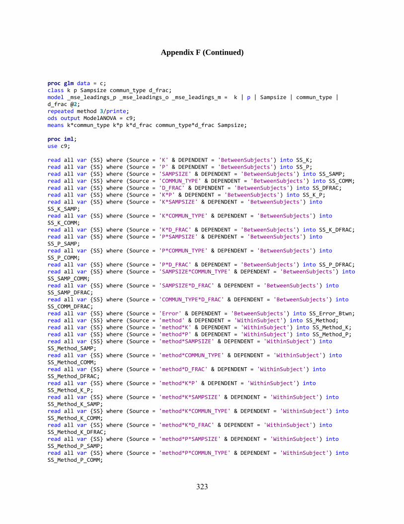
Appendix F (Continued)
323
proc glm data = c; class k p Sampsize commun_type d_frac; model _mse_leadings_p _mse_leadings_o _mse_leadings_m = k | p | Sampsize | commun_type | d_frac @2; repeated method 3/printe; ods output ModelANOVA = c9; means k*commun_type k*p k*d_frac commun_type*d_frac Sampsize; proc iml; use c9; read all var {SS} where (Source = 'K' & DEPENDENT = 'BetweenSubjects') into SS_K; read all var {SS} where (Source = 'P' & DEPENDENT = 'BetweenSubjects') into SS_P; read all var {SS} where (Source = 'SAMPSIZE' & DEPENDENT = 'BetweenSubjects') into SS_SAMP; read all var {SS} where (Source = 'COMMUN_TYPE' & DEPENDENT = 'BetweenSubjects') into SS_COMM; read all var {SS} where (Source = 'D_FRAC' & DEPENDENT = 'BetweenSubjects') into SS_DFRAC; read all var {SS} where (Source = 'K*P' & DEPENDENT = 'BetweenSubjects') into SS_K_P; read all var {SS} where (Source = 'K*SAMPSIZE' & DEPENDENT = 'BetweenSubjects') into SS_K_SAMP; read all var {SS} where (Source = 'K*COMMUN_TYPE' & DEPENDENT = 'BetweenSubjects') into SS_K_COMM; read all var {SS} where (Source = 'K*D_FRAC' & DEPENDENT = 'BetweenSubjects') into SS_K_DFRAC; read all var {SS} where (Source = 'P*SAMPSIZE' & DEPENDENT = 'BetweenSubjects') into SS_P_SAMP; read all var {SS} where (Source = 'P*COMMUN_TYPE' & DEPENDENT = 'BetweenSubjects') into SS_P_COMM; read all var {SS} where (Source = 'P*D_FRAC' & DEPENDENT = 'BetweenSubjects') into SS_P_DFRAC; read all var {SS} where (Source = 'SAMPSIZE*COMMUN_TYPE' & DEPENDENT = 'BetweenSubjects') into SS_SAMP_COMM; read all var {SS} where (Source = 'SAMPSIZE*D_FRAC' & DEPENDENT = 'BetweenSubjects') into SS_SAMP_DFRAC; read all var {SS} where (Source = 'COMMUN_TYPE*D_FRAC' & DEPENDENT = 'BetweenSubjects') into SS_COMM_DFRAC; read all var {SS} where (Source = 'Error' & DEPENDENT = 'BetweenSubjects') into SS_Error_Btwn; read all var {SS} where (Source = 'method' & DEPENDENT = 'WithinSubject') into SS_Method; read all var {SS} where (Source = 'method*K' & DEPENDENT = 'WithinSubject') into SS_Method_K; read all var {SS} where (Source = 'method*P' & DEPENDENT = 'WithinSubject') into SS_Method_P; read all var {SS} where (Source = 'method*SAMPSIZE' & DEPENDENT = 'WithinSubject') into SS_Method_SAMP; read all var {SS} where (Source = 'method*COMMUN_TYPE' & DEPENDENT = 'WithinSubject') into SS_Method_COMM; read all var {SS} where (Source = 'method*D_FRAC' & DEPENDENT = 'WithinSubject') into SS_Method_DFRAC; read all var {SS} where (Source = 'method*K*P' & DEPENDENT = 'WithinSubject') into SS_Method_K_P; read all var {SS} where (Source = 'method*K*SAMPSIZE' & DEPENDENT = 'WithinSubject') into SS_Method_K_SAMP; read all var {SS} where (Source = 'method*K*COMMUN_TYPE' & DEPENDENT = 'WithinSubject') into SS_Method_K_COMM; read all var {SS} where (Source = 'method*K*D_FRAC' & DEPENDENT = 'WithinSubject') into SS_Method_K_DFRAC; read all var {SS} where (Source = 'method*P*SAMPSIZE' & DEPENDENT = 'WithinSubject') into SS_Method_P_SAMP; read all var {SS} where (Source = 'method*P*COMMUN_TYPE' & DEPENDENT = 'WithinSubject') into SS_Method_P_COMM;
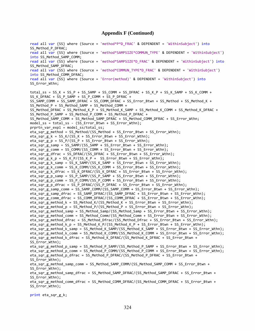
Appendix F (Continued)
324
read all var {SS} where (Source = 'method*P*D_FRAC' & DEPENDENT = 'WithinSubject') into SS_Method_P_DFRAC; read all var {SS} where (Source = 'method*SAMPSIZE*COMMUN_TYPE' & DEPENDENT = 'WithinSubject') into SS_Method_SAMP_COMM; read all var {SS} where (Source = 'method*SAMPSIZE*D_FRAC' & DEPENDENT = 'WithinSubject') into SS_Method_SAMP_DFRAC; read all var {SS} where (Source = 'method*COMMUN_TYPE*D_FRAC' & DEPENDENT = 'WithinSubject') into SS_Method_COMM_DFRAC; read all var {SS} where (Source = 'Error(method)' & DEPENDENT = 'WithinSubject') into SS_Error_Wthn; total_ss = SS_K + SS_P + SS_SAMP + SS_COMM + SS_DFRAC + SS_K_P + SS_K_SAMP + SS_K_COMM + SS_K_DFRAC + SS_P_SAMP + SS_P_COMM + SS_P_DFRAC + SS_SAMP_COMM + SS_SAMP_DFRAC + SS_COMM_DFRAC + SS_Error_Btwn + SS_Method + SS_Method_K + SS_Method_P + SS_Method_SAMP + SS_Method_COMM + SS_Method_DFRAC + SS_Method_K_P + SS_Method_K_SAMP + SS_Method_K_COMM + SS_Method_K_DFRAC + SS_Method_P_SAMP + SS_Method_P_COMM + SS_Method_P_DFRAC + SS_Method_SAMP_COMM + SS_Method_SAMP_DFRAC + SS_Method_COMM_DFRAC + SS_Error_Wthn; model_ss = total_ss ‐ (SS_Error_Btwn + SS_Error_Wthn); prprtn_var_expl = model_ss/total_ss; eta_sqr_g_method = SS_Method/(SS_Method + SS_Error_Btwn + SS_Error_Wthn); eta_sqr_g_k = SS_K/(SS_K + SS_Error_Btwn + SS_Error_Wthn); eta_sqr_g_p = SS_P/(SS_P + SS_Error_Btwn + SS_Error_Wthn); eta_sqr_g_samp = SS_SAMP/(SS_SAMP + SS_Error_Btwn + SS_Error_Wthn); eta_sqr_g_comm = SS_COMM/(SS_COMM + SS_Error_Btwn + SS_Error_Wthn); eta_sqr_g_dfrac = SS_DFRAC/(SS_DFRAC + SS_Error_Btwn + SS_Error_Wthn); eta_sqr_g_k_p = SS_K_P/(SS_K_P + SS_Error_Btwn + SS_Error_Wthn); eta_sqr_g_k_samp = SS_K_SAMP/(SS_K_SAMP + SS_Error_Btwn + SS_Error_Wthn); eta_sqr_g_k_comm = SS_K_COMM/(SS_K_COMM + SS_Error_Btwn + SS_Error_Wthn); eta_sqr_g_k_dfrac = SS_K_DFRAC/(SS_K_DFRAC + SS_Error_Btwn + SS_Error_Wthn); eta_sqr_g_p_samp = SS_P_SAMP/(SS_P_SAMP + SS_Error_Btwn + SS_Error_Wthn); eta_sqr_g_p_comm = SS_P_COMM/(SS_P_COMM + SS_Error_Btwn + SS_Error_Wthn); eta_sqr_g_p_dfrac = SS_P_DFRAC/(SS_P_DFRAC + SS_Error_Btwn + SS_Error_Wthn); eta_sqr_g_samp_comm = SS_SAMP_COMM/(SS_SAMP_COMM + SS_Error_Btwn + SS_Error_Wthn); eta_sqr_g_samp_dfrac = SS_SAMP_DFRAC/(SS_SAMP_DFRAC + SS_Error_Btwn + SS_Error_Wthn); eta_sqr_g_comm_dfrac = SS_COMM_DFRAC/(SS_COMM_DFRAC + SS_Error_Btwn + SS_Error_Wthn); eta_sqr_g_method_k = SS_Method_K/(SS_Method_K + SS_Error_Btwn + SS_Error_Wthn); eta_sqr_g_method_p = SS_Method_P/(SS_Method_P + SS_Error_Btwn + SS_Error_Wthn); eta_sqr_g_method_samp = SS_Method_Samp/(SS_Method_Samp + SS_Error_Btwn + SS_Error_Wthn); eta_sqr_g_method_comm = SS_Method_Comm/(SS_Method_Comm + SS_Error_Btwn + SS_Error_Wthn); eta_sqr_g_method_dfrac = SS_Method_Dfrac/(SS_Method_Dfrac + SS_Error_Btwn + SS_Error_Wthn); eta_sqr_g_method_k_p = SS_Method_K_P/(SS_Method_K_P + SS_Error_Btwn + SS_Error_Wthn); eta_sqr_g_method_k_samp = SS_Method_K_SAMP/(SS_Method_K_SAMP + SS_Error_Btwn + SS_Error_Wthn); eta_sqr_g_method_k_comm = SS_Method_K_COMM/(SS_Method_K_COMM + SS_Error_Btwn + SS_Error_Wthn); eta_sqr_g_method_k_dfrac = SS_Method_K_DFRAC/(SS_Method_K_DFRAC + SS_Error_Btwn + SS_Error_Wthn); eta_sqr_g_method_p_samp = SS_Method_P_SAMP/(SS_Method_P_SAMP + SS_Error_Btwn + SS_Error_Wthn); eta_sqr_g_method_p_comm = SS_Method_P_COMM/(SS_Method_P_COMM + SS_Error_Btwn + SS_Error_Wthn); eta_sqr_g_method_p_dfrac = SS_Method_P_DFRAC/(SS_Method_P_DFRAC + SS_Error_Btwn + SS_Error_Wthn); eta_sqr_g_method_samp_comm = SS_Method_SAMP_COMM/(SS_Method_SAMP_COMM + SS_Error_Btwn + SS_Error_Wthn); eta_sqr_g_method_samp_dfrac = SS_Method_SAMP_DFRAC/(SS_Method_SAMP_DFRAC + SS_Error_Btwn + SS_Error_Wthn); eta_sqr_g_method_comm_dfrac = SS_Method_COMM_DFRAC/(SS_Method_COMM_DFRAC + SS_Error_Btwn + SS_Error_Wthn); print eta_sqr_g_k;

Appendix F (Continued)
325
print eta_sqr_g_p; print eta_sqr_g_samp; print eta_sqr_g_comm; print eta_sqr_g_dfrac; print eta_sqr_g_k_p; print eta_sqr_g_k_samp; print eta_sqr_g_k_comm; print eta_sqr_g_k_dfrac; print eta_sqr_g_p_samp; print eta_sqr_g_p_comm; print eta_sqr_g_p_dfrac; print eta_sqr_g_samp_comm; print eta_sqr_g_samp_dfrac; print eta_sqr_g_comm_dfrac; print eta_sqr_g_method; print eta_sqr_g_method_k; print eta_sqr_g_method_p; print eta_sqr_g_method_samp; print eta_sqr_g_method_comm; print eta_sqr_g_method_dfrac; print eta_sqr_g_method_k; print eta_sqr_g_method_p; print eta_sqr_g_method_samp; print eta_sqr_g_method_comm; print eta_sqr_g_method_dfrac; print eta_sqr_g_method_k_p; print eta_sqr_g_method_k_samp; print eta_sqr_g_method_k_comm; print eta_sqr_g_method_k_dfrac; print eta_sqr_g_method_p_samp; print eta_sqr_g_method_p_comm; print eta_sqr_g_method_p_dfrac; print eta_sqr_g_method_samp_comm; print eta_sqr_g_method_samp_dfrac; print eta_sqr_g_method_comm_dfrac; print prprtn_var_expl; quit; proc glm data = c; class k p Sampsize commun_type d_frac; model _pattern_accuracy_p _pattern_accuracy_o _pattern_accuracy_m = k | p | Sampsize | commun_type | d_frac @2; repeated method 3/printe; ods output ModelANOVA = c10; means k*p k*commun_type k*sampsize p*commun_type sampsize*commun_type; proc iml; use c10; read all var {SS} where (Source = 'K' & DEPENDENT = 'BetweenSubjects') into SS_K; read all var {SS} where (Source = 'P' & DEPENDENT = 'BetweenSubjects') into SS_P; read all var {SS} where (Source = 'SAMPSIZE' & DEPENDENT = 'BetweenSubjects') into SS_SAMP; read all var {SS} where (Source = 'COMMUN_TYPE' & DEPENDENT = 'BetweenSubjects') into SS_COMM; read all var {SS} where (Source = 'D_FRAC' & DEPENDENT = 'BetweenSubjects') into SS_DFRAC; read all var {SS} where (Source = 'K*P' & DEPENDENT = 'BetweenSubjects') into SS_K_P;
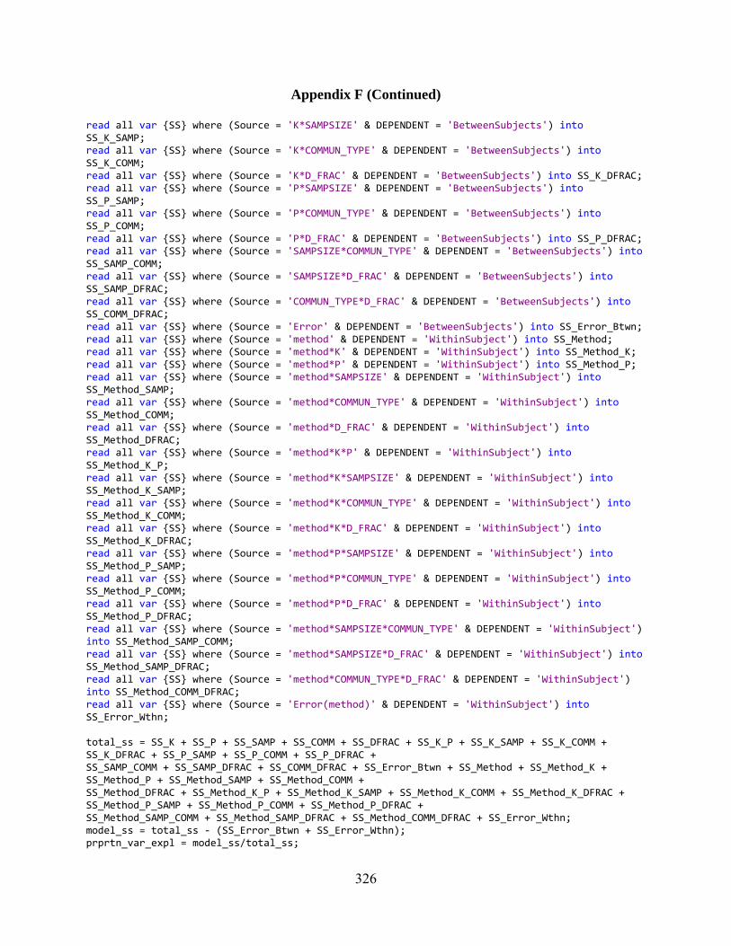
Appendix F (Continued)
326
read all var {SS} where (Source = 'K*SAMPSIZE' & DEPENDENT = 'BetweenSubjects') into SS_K_SAMP; read all var {SS} where (Source = 'K*COMMUN_TYPE' & DEPENDENT = 'BetweenSubjects') into SS_K_COMM; read all var {SS} where (Source = 'K*D_FRAC' & DEPENDENT = 'BetweenSubjects') into SS_K_DFRAC; read all var {SS} where (Source = 'P*SAMPSIZE' & DEPENDENT = 'BetweenSubjects') into SS_P_SAMP; read all var {SS} where (Source = 'P*COMMUN_TYPE' & DEPENDENT = 'BetweenSubjects') into SS_P_COMM; read all var {SS} where (Source = 'P*D_FRAC' & DEPENDENT = 'BetweenSubjects') into SS_P_DFRAC; read all var {SS} where (Source = 'SAMPSIZE*COMMUN_TYPE' & DEPENDENT = 'BetweenSubjects') into SS_SAMP_COMM; read all var {SS} where (Source = 'SAMPSIZE*D_FRAC' & DEPENDENT = 'BetweenSubjects') into SS_SAMP_DFRAC; read all var {SS} where (Source = 'COMMUN_TYPE*D_FRAC' & DEPENDENT = 'BetweenSubjects') into SS_COMM_DFRAC; read all var {SS} where (Source = 'Error' & DEPENDENT = 'BetweenSubjects') into SS_Error_Btwn; read all var {SS} where (Source = 'method' & DEPENDENT = 'WithinSubject') into SS_Method; read all var {SS} where (Source = 'method*K' & DEPENDENT = 'WithinSubject') into SS_Method_K; read all var {SS} where (Source = 'method*P' & DEPENDENT = 'WithinSubject') into SS_Method_P; read all var {SS} where (Source = 'method*SAMPSIZE' & DEPENDENT = 'WithinSubject') into SS_Method_SAMP; read all var {SS} where (Source = 'method*COMMUN_TYPE' & DEPENDENT = 'WithinSubject') into SS_Method_COMM; read all var {SS} where (Source = 'method*D_FRAC' & DEPENDENT = 'WithinSubject') into SS_Method_DFRAC; read all var {SS} where (Source = 'method*K*P' & DEPENDENT = 'WithinSubject') into SS_Method_K_P; read all var {SS} where (Source = 'method*K*SAMPSIZE' & DEPENDENT = 'WithinSubject') into SS_Method_K_SAMP; read all var {SS} where (Source = 'method*K*COMMUN_TYPE' & DEPENDENT = 'WithinSubject') into SS_Method_K_COMM; read all var {SS} where (Source = 'method*K*D_FRAC' & DEPENDENT = 'WithinSubject') into SS_Method_K_DFRAC; read all var {SS} where (Source = 'method*P*SAMPSIZE' & DEPENDENT = 'WithinSubject') into SS_Method_P_SAMP; read all var {SS} where (Source = 'method*P*COMMUN_TYPE' & DEPENDENT = 'WithinSubject') into SS_Method_P_COMM; read all var {SS} where (Source = 'method*P*D_FRAC' & DEPENDENT = 'WithinSubject') into SS_Method_P_DFRAC; read all var {SS} where (Source = 'method*SAMPSIZE*COMMUN_TYPE' & DEPENDENT = 'WithinSubject') into SS_Method_SAMP_COMM; read all var {SS} where (Source = 'method*SAMPSIZE*D_FRAC' & DEPENDENT = 'WithinSubject') into SS_Method_SAMP_DFRAC; read all var {SS} where (Source = 'method*COMMUN_TYPE*D_FRAC' & DEPENDENT = 'WithinSubject') into SS_Method_COMM_DFRAC; read all var {SS} where (Source = 'Error(method)' & DEPENDENT = 'WithinSubject') into SS_Error_Wthn; total_ss = SS_K + SS_P + SS_SAMP + SS_COMM + SS_DFRAC + SS_K_P + SS_K_SAMP + SS_K_COMM + SS_K_DFRAC + SS_P_SAMP + SS_P_COMM + SS_P_DFRAC + SS_SAMP_COMM + SS_SAMP_DFRAC + SS_COMM_DFRAC + SS_Error_Btwn + SS_Method + SS_Method_K + SS_Method_P + SS_Method_SAMP + SS_Method_COMM + SS_Method_DFRAC + SS_Method_K_P + SS_Method_K_SAMP + SS_Method_K_COMM + SS_Method_K_DFRAC + SS_Method_P_SAMP + SS_Method_P_COMM + SS_Method_P_DFRAC + SS_Method_SAMP_COMM + SS_Method_SAMP_DFRAC + SS_Method_COMM_DFRAC + SS_Error_Wthn; model_ss = total_ss ‐ (SS_Error_Btwn + SS_Error_Wthn); prprtn_var_expl = model_ss/total_ss;

Appendix F (Continued)
327
eta_sqr_g_method = SS_Method/(SS_Method + SS_Error_Btwn + SS_Error_Wthn); eta_sqr_g_k = SS_K/(SS_K + SS_Error_Btwn + SS_Error_Wthn); eta_sqr_g_p = SS_P/(SS_P + SS_Error_Btwn + SS_Error_Wthn); eta_sqr_g_samp = SS_SAMP/(SS_SAMP + SS_Error_Btwn + SS_Error_Wthn); eta_sqr_g_comm = SS_COMM/(SS_COMM + SS_Error_Btwn + SS_Error_Wthn); eta_sqr_g_dfrac = SS_DFRAC/(SS_DFRAC + SS_Error_Btwn + SS_Error_Wthn); eta_sqr_g_k_p = SS_K_P/(SS_K_P + SS_Error_Btwn + SS_Error_Wthn); eta_sqr_g_k_samp = SS_K_SAMP/(SS_K_SAMP + SS_Error_Btwn + SS_Error_Wthn); eta_sqr_g_k_comm = SS_K_COMM/(SS_K_COMM + SS_Error_Btwn + SS_Error_Wthn); eta_sqr_g_k_dfrac = SS_K_DFRAC/(SS_K_DFRAC + SS_Error_Btwn + SS_Error_Wthn); eta_sqr_g_p_samp = SS_P_SAMP/(SS_P_SAMP + SS_Error_Btwn + SS_Error_Wthn); eta_sqr_g_p_comm = SS_P_COMM/(SS_P_COMM + SS_Error_Btwn + SS_Error_Wthn); eta_sqr_g_p_dfrac = SS_P_DFRAC/(SS_P_DFRAC + SS_Error_Btwn + SS_Error_Wthn); eta_sqr_g_samp_comm = SS_SAMP_COMM/(SS_SAMP_COMM + SS_Error_Btwn + SS_Error_Wthn); eta_sqr_g_samp_dfrac = SS_SAMP_DFRAC/(SS_SAMP_DFRAC + SS_Error_Btwn + SS_Error_Wthn); eta_sqr_g_comm_dfrac = SS_COMM_DFRAC/(SS_COMM_DFRAC + SS_Error_Btwn + SS_Error_Wthn); eta_sqr_g_method_k = SS_Method_K/(SS_Method_K + SS_Error_Btwn + SS_Error_Wthn); eta_sqr_g_method_p = SS_Method_P/(SS_Method_P + SS_Error_Btwn + SS_Error_Wthn); eta_sqr_g_method_samp = SS_Method_Samp/(SS_Method_Samp + SS_Error_Btwn + SS_Error_Wthn); eta_sqr_g_method_comm = SS_Method_Comm/(SS_Method_Comm + SS_Error_Btwn + SS_Error_Wthn); eta_sqr_g_method_dfrac = SS_Method_Dfrac/(SS_Method_Dfrac + SS_Error_Btwn + SS_Error_Wthn); eta_sqr_g_method_k_p = SS_Method_K_P/(SS_Method_K_P + SS_Error_Btwn + SS_Error_Wthn); eta_sqr_g_method_k_samp = SS_Method_K_SAMP/(SS_Method_K_SAMP + SS_Error_Btwn + SS_Error_Wthn); eta_sqr_g_method_k_comm = SS_Method_K_COMM/(SS_Method_K_COMM + SS_Error_Btwn + SS_Error_Wthn); eta_sqr_g_method_k_dfrac = SS_Method_K_DFRAC/(SS_Method_K_DFRAC + SS_Error_Btwn + SS_Error_Wthn); eta_sqr_g_method_p_samp = SS_Method_P_SAMP/(SS_Method_P_SAMP + SS_Error_Btwn + SS_Error_Wthn); eta_sqr_g_method_p_comm = SS_Method_P_COMM/(SS_Method_P_COMM + SS_Error_Btwn + SS_Error_Wthn); eta_sqr_g_method_p_dfrac = SS_Method_P_DFRAC/(SS_Method_P_DFRAC + SS_Error_Btwn + SS_Error_Wthn); eta_sqr_g_method_samp_comm = SS_Method_SAMP_COMM/(SS_Method_SAMP_COMM + SS_Error_Btwn + SS_Error_Wthn); eta_sqr_g_method_samp_dfrac = SS_Method_SAMP_DFRAC/(SS_Method_SAMP_DFRAC + SS_Error_Btwn + SS_Error_Wthn); eta_sqr_g_method_comm_dfrac = SS_Method_COMM_DFRAC/(SS_Method_COMM_DFRAC + SS_Error_Btwn + SS_Error_Wthn); print eta_sqr_g_k; print eta_sqr_g_p; print eta_sqr_g_samp; print eta_sqr_g_comm; print eta_sqr_g_dfrac; print eta_sqr_g_k_p; print eta_sqr_g_k_samp; print eta_sqr_g_k_comm; print eta_sqr_g_k_dfrac; print eta_sqr_g_p_samp; print eta_sqr_g_p_comm; print eta_sqr_g_p_dfrac; print eta_sqr_g_samp_comm; print eta_sqr_g_samp_dfrac; print eta_sqr_g_comm_dfrac; print eta_sqr_g_method; print eta_sqr_g_method_k; print eta_sqr_g_method_p; print eta_sqr_g_method_samp; print eta_sqr_g_method_comm; print eta_sqr_g_method_dfrac;

Appendix F (Continued)
328
print eta_sqr_g_method_k; print eta_sqr_g_method_p; print eta_sqr_g_method_samp; print eta_sqr_g_method_comm; print eta_sqr_g_method_dfrac; print eta_sqr_g_method_k_p; print eta_sqr_g_method_k_samp; print eta_sqr_g_method_k_comm; print eta_sqr_g_method_k_dfrac; print eta_sqr_g_method_p_samp; print eta_sqr_g_method_p_comm; print eta_sqr_g_method_p_dfrac; print eta_sqr_g_method_samp_comm; print eta_sqr_g_method_samp_dfrac; print eta_sqr_g_method_comm_dfrac; print prprtn_var_expl; quit; /*Box and Whisker plots*/ data c1; set c; d_frac_prct = d_frac*100; data d; set c1; K_x_P = k||'‐'||p; K_x_N = k||'‐'||sampsize; K_x_H = k||'‐'||commun_type; K_x_D = k||'‐'||d_frac_prct; P_x_H = p||'‐'||commun_type; P_x_N = p||'‐'||sampsize; N_x_H = sampsize||'‐'||commun_type; H_x_D = commun_type||'‐'||d_frac_prct; data d1; set d; Loading_sensitivity = _ok_load_p; General_agreement = _Pattern_Accuracy30_p; Per_element_agreement = _pattern_accuracy_p; Total_agreement = _Perfect_Accuracy_p; Mean_phi = _meanphi_p; Factor_score_R = _R_Fscores_p; Bias = _bias_loadings_p; RMSE = _mse_leadings_p; method = 'PAF'; data d2; set d; Loading_sensitivity = _ok_load_o; General_agreement = _Pattern_Accuracy30_o; Per_element_agreement = _pattern_accuracy_o; Total_agreement = _Perfect_Accuracy_o; Mean_phi = _meanphi_o; Factor_score_R = _R_Fscores_o; Bias = _bias_loadings_o;

Appendix F (Continued)
329
RMSE = _mse_leadings_o; method = 'OLS'; data d3; set d; Loading_sensitivity = _ok_load_m; General_agreement = _Pattern_Accuracy30_m; Per_element_agreement = _pattern_accuracy_m; Total_agreement = _Perfect_Accuracy_m; Mean_phi = _meanphi_m; Factor_score_R = _R_Fscores_m; Bias = _bias_loadings_m; RMSE = _mse_leadings_m; method = 'MAX'; data d_comb; set d1; proc append base = d_comb data = d2 force; proc append base = d_comb data = d3 force; proc sort data = d_comb; by method; proc means data = d_comb; var Loading_sensitivity General_agreement Per_element_agreement Total_agreement Mean_phi Factor_score_R Bias RMSE; by method; data d4; set d_comb; xK_x_P = compress(K_x_P); xK_x_N = compress(K_x_N); xK_x_H = compress(K_x_H); xK_x_D = compress(K_x_D); xP_x_N = compress(P_x_N); xP_x_H = compress(P_x_H); xN_x_H = compress(N_x_H); xH_x_D = compress(H_x_D); method_x_N = method||'‐'||sampsize; /*K by P Interaction Boxplots*/ proc sort data = d4; by Method K_x_P; proc boxplot data = d4; plot Loading_sensitivity*xK_x_P (Method)/npanelpos = 27 turnhlabels blockpos = 1 boxstyle = schematic; label xK_x_P = 'Number of Factors by Number of Observed Variables Interaction'; label method = 'Factor Extraction Method'; label Loading_sensitivity ='Loading Sensitivity';

Appendix F (Continued)
330
proc boxplot data = d4; plot General_agreement*xK_x_P (Method)/npanelpos = 27 turnhlabels blockpos = 1 boxstyle = schematic; label xK_x_P = 'Number of Factors by Number of Observed Variables Interaction'; label method = 'Factor Extraction Method'; label General_agreement ='General Pattern Agreement'; proc boxplot data = d4; plot Per_element_agreement*xK_x_P (Method)/npanelpos = 27 turnhlabels blockpos = 1 boxstyle = schematic; label xK_x_P = 'Number of Factors by Number of Observed Variables Interaction'; label method = 'Factor Extraction Method'; label Per_element_agreement ='Per Element Agreement'; proc boxplot data = d4; plot Total_agreement*xK_x_P (Method)/npanelpos = 27 turnhlabels blockpos = 1 boxstyle = schematic; label xK_x_P = 'Number of Factors by Number of Observed Variables Interaction'; label method = 'Factor Extraction Method'; label Total_agreement ='Total Agreement'; proc boxplot data = d4; plot Mean_phi*xK_x_P (Method)/npanelpos = 27 turnhlabels blockpos = 1 boxstyle = schematic; label xK_x_P = 'Number of Factors by Number of Observed Variables Interaction'; label method = 'Factor Extraction Method'; label Mean_phi ='Mean Phi Values'; proc boxplot data = d4; plot Factor_score_R*xK_x_P (Method)/npanelpos = 27 turnhlabels blockpos = 1 boxstyle = schematic; label xK_x_P = 'Number of Factors by Number of Observed Variables Interaction'; label method = 'Factor Extraction Method'; label Factor_score_R ='Factor Score Correlations'; proc boxplot data = d4; plot Bias*xK_x_P (Method)/npanelpos = 27 turnhlabels blockpos = 1 boxstyle = schematic; label xK_x_P = 'Number of Factors by Number of Observed Variables Interaction'; label method = 'Factor Extraction Method'; label Bias ='Factor Loading Bias'; proc boxplot data = d4; plot RMSE*xK_x_P (Method)/npanelpos = 27 turnhlabels blockpos = 1 boxstyle = schematic; label xK_x_P = 'Number of Factors by Number of Observed Variables Interaction'; label method = 'Factor Extraction Method'; label RMSE ='RMSE'; /*K by N Interaction Boxplots*/ proc sort data = d4; by Method K_x_N; proc boxplot data = d4; plot Per_element_agreement*xK_x_N (Method)/npanelpos = 36 turnhlabels blockpos = 1 boxstyle = schematic; label xK_x_N = 'Number of Factors by Sample Size Interaction';
Appendix F (Continued)
331
label method = 'Factor Extraction Method'; label Per_element_agreement ='Per Element Agreement'; proc boxplot data = d4; plot Total_agreement*xK_x_N (Method)/npanelpos = 36 turnhlabels blockpos = 1 boxstyle = schematic; label xK_x_N = 'Number of Factors by Sample Size Interaction'; label method = 'Factor Extraction Method'; label Total_agreement ='Total Agreement'; proc boxplot data = d4; plot Mean_phi*xK_x_N (Method)/npanelpos = 36 turnhlabels blockpos = 1 boxstyle = schematic; label xK_x_N = 'Number of Factors by Sample Size Interaction'; label method = 'Factor Extraction Method'; label Mean_phi ='Mean Phi Values'; proc boxplot data = d4; plot Factor_score_R*xK_x_N (Method)/npanelpos = 36 turnhlabels blockpos = 1 boxstyle = schematic; label xK_x_N = 'Number of Factors by Sample Size Interaction'; label method = 'Factor Extraction Method'; label Factor_score_R ='Factor Score Correlationss'; proc boxplot data = d4; plot Bias*xK_x_N (Method)/npanelpos = 36 turnhlabels blockpos = 1 boxstyle = schematic; label xK_x_N = 'Number of Factors by Sample Size Interaction'; label method = 'Factor Extraction Method'; label Bias ='Factor Loading Bias'; /*K by H Interaction Boxplots*/ proc sort data = d4; by Method K_x_H; proc boxplot data = d4; plot Loading_sensitivity*xK_x_H (Method)/npanelpos = 27 turnhlabels blockpos = 1 boxstyle = schematic; label xK_x_H = 'Number of Factors by Communality Level (Low=1, Wide=2, High=3) Interaction'; label method = 'Factor Extraction Method'; label Loading_sensitivity ='Loading Sensitivity'; proc boxplot data = d4; plot General_agreement*xK_x_H (Method)/npanelpos = 27 turnhlabels blockpos = 1 boxstyle = schematic; label xK_x_H = 'Number of Factors by Communality Level (Low=1, Wide=2, High=3) Interaction'; label method = 'Factor Extraction Method'; label General_agreement ='General Pattern Agreement'; proc boxplot data = d4; plot Per_element_agreement*xK_x_H (Method)/npanelpos = 27 turnhlabels blockpos = 1 boxstyle = schematic;

Appendix F (Continued)
332
label xK_x_H = 'Number of Factors by Communality Level (Low=1, Wide=2, High=3) Interaction'; label method = 'Factor Extraction Method'; label Per_element_agreement ='Per Element Agreement'; proc boxplot data = d4; plot Factor_score_R*xK_x_H (Method)/npanelpos = 27 turnhlabels blockpos = 1 boxstyle = schematic; label xK_x_H = 'Number of Factors by Communality Level (Low=1, Wide=2, High=3) Interaction'; label method = 'Factor Extraction Method'; label Factor_score_R ='Factor Score Correlations'; proc boxplot data = d4; plot Bias*xK_x_H (Method)/npanelpos = 27 turnhlabels blockpos = 1 boxstyle = schematic; label xK_x_H = 'Number of Factors by Communality Level (Low=1, Wide=2, High=3) Interaction'; label method = 'Factor Extraction Method'; label Bias ='Factor Loading Bias'; proc boxplot data = d4; plot RMSE*xK_x_H (Method)/npanelpos = 27 turnhlabels blockpos = 1 boxstyle = schematic; label xK_x_H = 'Number of Factors by Communality Level (Low=1, Wide=2, High=3) Interaction'; label method = 'Factor Extraction Method'; label RMSE ='RMSE'; /*K by D Interaction Boxplots*/ proc sort data = d4; by Method K_x_D; proc boxplot data = d4; plot Loading_sensitivity*xK_x_D (Method)/npanelpos = 45 turnhlabels blockpos = 1 boxstyle = schematic; label xK_x_D = 'Number of Factors by Dichotomization (as a Percentage of Observed Variables) Interaction'; label method = 'Factor Extraction Method'; label Loading_sensitivity ='Loading Sensitivity'; proc boxplot data = d4; plot Mean_phi*xK_x_D (Method)/npanelpos = 45 turnhlabels blockpos = 1 boxstyle = schematic; label xK_x_D = 'Number of Factors by Dichotomization (as a Percentage of Observed Variables) Interaction'; label method = 'Factor Extraction Method'; label Mean_phi ='Mean Phi Values'; proc boxplot data = d4; plot Bias*xK_x_D (Method)/npanelpos = 45 turnhlabels blockpos = 1 boxstyle = schematic; label xK_x_D = 'Number of Factors by Dichotomization (as a Percentage of Observed Variables) Interaction'; label method = 'Factor Extraction Method'; label Bias ='Factor Loading Bias'; proc boxplot data = d4; plot RMSE*xK_x_D (Method)/npanelpos = 45 turnhlabels blockpos = 1 boxstyle = schematic;

Appendix F (Continued)
333
label xK_x_D = 'Number of Factors by Dichotomization (as a Percentage of Observed Variables)Interaction'; label method = 'Factor Extraction Method'; label RMSE ='RMSE'; /*P by N Interaction Boxplots*/ proc sort data = d4; by Method P_x_N; proc boxplot data = d4; plot Total_agreement*xP_x_N (Method)/npanelpos = 36 turnhlabels blockpos = 1 boxstyle = schematic; label xP_x_N = 'Number of Observed Variables by Sample Size Interaction'; label method = 'Factor Extraction Method'; label Total_agreement ='Total Agreement'; /*P by H Interaction Boxplots*/ proc sort data = d4; by Method P_x_H; proc boxplot data = d4; plot Loading_sensitivity*xP_x_H (Method)/npanelpos = 27 turnhlabels blockpos = 1 boxstyle = schematic; label xP_x_H = 'Number of Observed Variables by Communality Level (Low=1, Wide=2, High=3) Interaction'; label method = 'Factor Extraction Method'; label Loading_sensitivity ='Loading Sensitivity'; proc boxplot data = d4; plot General_agreement*xP_x_H (Method)/npanelpos = 27 turnhlabels blockpos = 1 boxstyle = schematic; label xP_x_H = 'Number of Observed Variables by Communality Level (Low=1, Wide=2, High=3) Interaction'; label method = 'Factor Extraction Method'; label General_agreement ='General Pattern Agreement'; proc boxplot data = d4; plot Per_element_agreement*xP_x_H (Method)/npanelpos = 27 turnhlabels blockpos = 1 boxstyle = schematic; label xP_x_H = 'Number of Observed Variables by Communality Level (Low=1, Wide=2, High=3) Interaction'; label method = 'Factor Extraction Method'; label Per_element_agreement ='Per Element Agreement'; proc boxplot data = d4; plot Factor_score_R*xP_x_H (Method)/npanelpos = 27 turnhlabels blockpos = 1 boxstyle = schematic; label xP_x_H = 'Number of Observed Variables by Communality Level (Low=1, Wide=2, High=3) Interaction'; label method = 'Factor Extraction Method'; label Factor_score_R ='Factor Score Correlations'; /*N by H Interaction Boxplots*/ proc sort data = d4;

Appendix F (Continued)
334
by Method N_x_H; proc boxplot data = d4; plot General_agreement*xN_x_H (Method)/npanelpos = 36 turnhlabels blockpos = 1 boxstyle = schematic; label xN_x_H = 'Sample Size by Communality Level (Low=1, Wide=2, High=3) Interaction'; label method = 'Factor Extraction Method'; label General_agreement ='General Pattern Agreement'; proc boxplot data = d4; plot Per_element_agreement*xN_x_H (Method)/npanelpos = 36 turnhlabels blockpos = 1 boxstyle = schematic; label xN_x_H = 'Sample Size by Communality Level (Low=1, Wide=2, High=3) Interaction'; label method = 'Factor Extraction Method'; label Per_element_agreement ='Per Element Agreement'; proc boxplot data = d4; plot Mean_phi*xN_x_H (Method)/npanelpos = 36 turnhlabels blockpos = 1 boxstyle = schematic; label xN_x_H = 'Sample Size by Communality Level (Low=1, Wide=2, High=3) Interaction'; label method = 'Factor Extraction Method'; label Mean_phi ='Mean Phi Values'; /*H by D Interaction Boxplots*/ proc sort data = d4; by Method H_x_D; proc boxplot data = d4; plot Mean_phi*xH_x_D (Method)/npanelpos = 45 turnhlabels blockpos = 1 boxstyle = schematic; label xH_x_D = 'Communality Level (Low=1, Wide=2, High=3) by Dichotomization (as a Percentage of Observed Variables) Interaction'; label method = 'Factor Extraction Method'; label Mean_phi ='Mean Phi Values'; proc boxplot data = d4; plot RMSE*xH_x_D (Method)/npanelpos = 45 turnhlabels blockpos = 1 boxstyle = schematic; label xH_x_D = 'Communality Level (Low=1, Wide=2, High=3) by Dichotomization (as a Percentage of Observed Variables) Interaction'; label method = 'Factor Extraction Method'; label RMSE ='RMSE'; /*sample size main effect*/ data d5; set d4; xMethod_x_N = compress(Method_x_n); proc sort data = d5; by xMethod_x_N;

Appendix F (Continued)
335
proc boxplot data = d5; plot RMSE*xMethod_x_N/boxstyle = schematic; label xMethod_x_N = 'Method by Sample Size Main Effect'; label RMSE ='RMSE'; run; quit;