Embed Size (px)
Citation preview

An Analysis of the Effect of Consolidation on Student Achievement:
Evidence from Arkansas
Jonathan N. Mills*
University of Arkansas
Josh B. McGee
Laura and John Arnold Foundation
Jay P. Greene
University of Arkansas
EDRE Working Paper No. 2013-02
Last Updated March 2013
Please Do Not Cite without Author Permission
Abstract
The consolidation of schools and districts has been one of the most widespread education
reforms of the last century; however, surprisingly little research has directly investigated the
effectiveness of consolidation as a reform strategy. We provide new ev
when policymakers required
the consolidation of all districts with average daily attendance of fewer than 350 students for two
consecutive years. Using both regres models, we
attempt to tease out the effects of state mandated consolidation. In general, we find that
consolidation has a positive, yet practically insignificant performance impact on students from
consolidating districts and a small negative performance impact for students in districts that
merged with consolidating districts. School closure, a consolidation related phenomenon, is
found to have a strong negative impact on affected students.
Key Words: consolidation, district size, regression discontinuity, instrumental variables
* Corresponding author: Address: 208 Graduate Education Building, University of Arkansas, Fayetteville AR,
72701; Tel.:1-479-575-3172; Fax: 1-479-575-3196. E-mail address: [email protected]

1
1. Introduction
District consolidation has been one of the most prevalent education reforms over the last
century. Between 1940 and 2008, for example, the number of public school districts in the U.S.
declined substantially from 117,108 to 13,924.1
Andrews, Duncombe, and Yinger
school size on student outcomes
but the results on the
size of high schools are more ambiguous.
Virtually all of this research examined existing variat
and
Nitta, Holley, and Wrobel, 2010) have focused on out
But all of these studies, both those examining size
as well as those examining consolidation-induced changes in size, are susceptible to endogeneity
issues
their academic quality. Estimates of the
effects of scale on achievemen the fact that scale is also a function of achievement.
1 Source NCES's 2009 Digest of Education Statistics:
http://nces.ed.gov/programs/digest/d09/tables/dt09_086.asp?referrer=list

2
are
This paper contributes to the
that occur
bright-line
discontinuity provides an excellent source of exogenous v learn about the effects
of consolidation and scale in education.
The remainder of this paper proceeds as follows. Section 2 reviews the literature on
district consolidation and returns to scale in education. Section 3 details ’ mandated
district consolidation legislation, Arkansas Act 60. In Section 4, we outline the data used in this
study and Section 5 includes descriptions of the empirical methods employed in this paper as
well as our results. Section 6 concludes the paper with a summary of our findings.
2. Review of Literature on Consolidation in Public Schooling
The ten-fold reduction in the number of public school districts in the U.S. since 1940 has
largely been motivated by arguments focusing on economies of scale. As Duncombe and Yinger
(2007) note, consolidation is often proposed as a means to take advantage of economies of scale
by spreading administrative costs over a larger student body without diminishing quality. In
addition, consolidation proponents claim that larger districts can employ a more efficient
teaching workforce by allowing teachers to specialize within a particular discipline while also
allowing for more collaboration among a more diverse teaching body. At the same time,
consolidation policies are not without detractors. For example, Duncombe and Yinger (2007)
note consolidation opponents argue that larger districts experience diseconomies of scale

3
stemming from higher transportation costs, a stronger union presence, and less buy-in from
parents, students, and teachers. Nevertheless, despite the push back of consolidation opponents,
district consolidation has clearly affected the overwhelming majority of districts and
communities in the U.S. in the last century.
Beyond these arguments, several researchers have highlighted a multitude of social and
economic factors that act as barriers to consolidation. Alesina, Baqir, and Hoxby (2004) find that
income and racial heterogeneity are important determinants in the number and size of school
districts. Furthermore, Brasington (2003) finds that the difference in size between two districts
increases the likelihood of choosing to consolidate for a large district and decreases this
likelihood for smaller districts. District perspectives aside, the large-scale reduction in the
number of school districts in the U.S. is evidence that policy makers have tended to favor the
arguments for consolidation, focusing on the cost benefits that economies of scale arguments
imply. In many states policy makers have employed significant fiscal and regulatory incentives
to encourage district mergers. Tight budgetary conditions at the state and local levels are sure to
fuel discussion of further consolidation in an effort to cut cost.
’ , relatively few studies have been able to directly
examine the impact of consolidation primarily due to data limitations. Instead, the majority of the
empirical research has focused on the impact of consolidation indirectly by confirming the
validity of the underlying theory: economies of scale. This body of research has examined effects
both at the district and school level, with the majority of recent evidence supporting economies
of scale at the district level and diseconomies of scale at the school level.2
2 For reviews of the literature on economies of scale in district and school size, see Andrews, Duncombe, and Yinger
(2002) and Leithwood and Jantzi (2009), respectively.

4
The few studies that directly examine the effects of scale on student performance are
limited and their results are quite mixed. Walberg and Fowler (1987) examine 500 school
districts in New Jersey using a production function methodology, finding consistent evidence of
moderate diseconomies of scale. In contrast, Berry and West (2008) examine data on three
cohorts of students born between 1920 and 1940 from the Public-Use Micro-Sample of the 1980
U.S. Census. They find that an increase in district enrollment of 947 students is associated with a
2.1 percent increase in future earnings and is not harmful to student achievement.
The primary issue facing the study of both consolidation and economies of scale in
education is the fact that district and school enrollment is rarely exogenous. The studies reviewed
above are largely cross-sectional in nature, and the models they employ fail to fully account for
the fact that size and achievement are likely related. Kuziemko (2006) is one of the only studies
to appropriately address this issue. The author employs a two stage least squares (2SLS)
approach exploiting shocks in enrollment due to school openings, closings, and mergers to
investigate the effect of size on student achievement. Kuziemko finds insignificant results in the
first year after an enrollment change. However, she finds significant, negative effects on both
attendance and math scores in the second and third years after a change.
Two works that have recently attempted to directly examine the effects of consolidation.
Duncombe and Yinger (2007) use a cost function approach to examine fiscal impacts of
consolidation using a matched panel of rural districts in New York. They find evidence of
significant cost savings at the district level. The authors found that doubling the enrollment of a
300 student district would result in a 61.7 percent reduction in operating costs, and likewise that
a similar doubling for a 1,500 student district would result in 49.6 percent reduction. The authors
found adjustment costs, largely accounted for by capital spending, lowered the total savings

5
somewhat, but the overall effect remained. While this study is able to investigate the direct
impacts of consolidation through the use of a matched panel, it fails to appropriately control for
endogeneity of enrollment.
Nitta, Holley, and Wrobel (2010) conducted surveys in four districts in Arkansas that
experienced mergers to gain a first-hand understanding of how consolidation impacted the
students and teachers involved. While the results were fairly diverse across the districts, the
authors proposed two general findings: (1) students tended to adapt much better than teachers,
and (2) nearly all people involved experienced at least some type of benefit from consolidation.
Although the small sample size and reliance on survey data make it hard to generalize these
findings to all consolidations, they provide a guide for expectations in our study of consolidation
in Arkansas.
The existing empirical research on the impacts of consolidation broadly suggests
economies of scale at the district level and diseconomies of scale at the school level on a variety
of measures. Unfortunately, the simple fact that districts chose to consolidate implies a selection
bias that is generally not addressed in the empirical literature. Furthermore, few studies have
directly examined the impact of district consolidation on student achievement, an outcome of
importance to policymakers. Fortunately, a mandatory consolidation policy introduced in
Arkansas in 2004 provides us with a unique opportunity to study the impacts of consolidation
while avoiding issues involved with the endogeneity of the consolidation decision.
3. Consolidation in Arkansas: Act 60
The latest wave of school consolidation in Arkansas arose in response to school finance
litigation that occurred throughout the late 1990s and early 2000s. The decade long litigation
C ’

6
system was unconstitutional in Lake View School District vs. Huckabee. Governor Mike
’ State Legislature in the Second
Extraordinary Session of 2003. Governor Huckabee proposed large-scale school district
consolidation to reduce district administrative costs and provide greater educational opportunity
for students. Governor Huckabee's original proposal would have resulted in three-fold reduction
in the number of districts in Arkansas from just over 300 to around 100. Compromise legislation
was passed in early 2004. The Public Education Reorganization Act, Arkansas Act 60, required
any district with average daily attendance of fewer than 350 students for two consecutive years
to consolidate.3
The final enrollment threshold of 350, while not as drastic as the Governors original
proposal, did result in a substantial number of district consolidations in the years that followed.
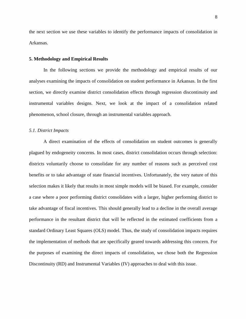
Table 1 presents the number of district consolidations occurring since the 2004-05 school year.
While the majority of district consolidations occurred immediately following the passage of Act
60, the legislation continues to affect Arkansas education as enrolments decline in rural districts.
[Table 1 here]
While Act 60 does not specifically require school closure following a consolidation,
closures often occur in order to eliminate school and grade duplication and to take advantage of
other perceived economies of scale. Table 2 presents the number of school closures that have
occurred following a district consolidation. Unsurprisingly, consolidation has had a non-trivial
impact on school closures.
[Table 2 here]
3 For the remainder of this paper, when we refer to Act 60 or an enrollment level of 350, we are specifically
’ -year average enrollment.

7
4. Data
Our analysis makes use of a rich panel of demographic and performance data for all
students who took the Arkansas mathematics and literacy Benchmark exams between the 2001-
02 and 2009-11 school years. Arkansas did not provide examinations for all grades between the
third and eighth grade until the 2004-05 school year. Thus, ’
current and prior test score can at most use records beginning in the 2003-04 school year. While
the performance of our models should not be strongly affected by these missing data, we do
caution the reader to take these data limitations into account when interpreting our findings.
We also have data on district and school enrollment collected from the Arkansas
Department of Education (ADE) as well as information on district consolidation and school
closure compiled with the help of ADE and district officials. Throughout, we identify post-Act
60 districts that were involved in mergers as one of three types: districts with two-year average
enrollment less t “ ” two-year
“ ”
“ ” We merged these data on key
variables to create a master panel that includes roughly 200,000 records per year across grades
three through eight with multiple records for students across school years.
We identify students as consolidated if they were in a district that was forced to
consolidate in the prior year, and they continue to be identified as such for the remainder of their
appearance in the data. We identify students as being in receiving districts if they are enrolled in
districts that merged with a consolidated district. Similar to the consolidated children, these
students are identified as receiving students for the remainder of their appearance in the data. In
8
the next section we use these variables to identify the performance impacts of consolidation in
Arkansas.
5. Methodology and Empirical Results
In the following sections we provide the methodology and empirical results of our
analyses examining the impacts of consolidation on student performance in Arkansas. In the first
section, we directly examine district consolidation effects through regression discontinuity and
instrumental variables designs. Next, we look at the impact of a consolidation related
phenomenon, school closure, through an instrumental variables approach.
5.1. District Impacts
A direct examination of the effects of consolidation on student outcomes is generally
plagued by endogeneity concerns. In most cases, district consolidation occurs through selection:
districts voluntarily choose to consolidate for any number of reasons such as perceived cost
benefits or to take advantage of state financial incentives. Unfortunately, the very nature of this
selection makes it likely that results in most simple models will be biased. For example, consider
a case where a poor performing district consolidates with a larger, higher performing district to
take advantage of fiscal incentives. This should generally lead to a decline in the overall average
performance in the resultant district that will be reflected in the estimated coefficients from a
standard Ordinary Least Squares (OLS) model. Thus, the study of consolidation impacts requires
the implementation of methods that are specifically geared towards addressing this concern. For
the purposes of examining the direct impacts of consolidation, we chose both the Regression
Discontinuity (RD) and Instrumental Variables (IV) approaches to deal with this issue.

9
5.1.1. Regression Discontinuity Model
First, we examine the impacts of consolidation on student performance in the likely
presence of endogeneity bias through a standard RD approach.4 The explicit enrollment cut-off
designated by Act 60 allows us to employ a fuzzy RD model whereby students in districts with
pre-Act 60 two-year average enrollment of less than 350 students are assigned to the treatment
group and students in the remaining districts represent the control group. Our design is “fuzzy”
because attending a district with average enrollment fewer than 350 students prior to Act 60 is
not a perfect predictor of receiving the consolidation treatment. We investigated the
misclassification of students to the treatment group by estimating a linear probability model
where pre-Act 60 district enrollment was the sole regressor. We then used our estimation results
to predict the probability of assignment to the treatment group. Our results show some overlap
between the treatment and control groups. Specifically, 90 percent of students who did not
receive the treatment had predicted probabilities of consolidation less than 0.27 while about 10
percent of students who actually the consolidation treatment had predicted probability of less
than 0.25.
In choosing the RD
slightly greater than the Act 60 mandated cut-off are essentially the same as students in the
consolidated districts. We estimated the model specified in equation 5.1 below.
(5.1)
In this equation Y represents student i's standardized scale score on a state exam, C is an
indicator variable for consolidation due to Act 60, E is vector of linear and higher-order
4 For a more general treatment of regression discontinuity models, see Imbens, G.W. & Lemieux, T. (2008).
Regression Discontinuity Designs: A Guide to Practice. Journal of Econometrics, 142.

10
transformations of the two-year average enrollment for student i's district5, X is a vector of
individual level controls (ethnicity, gender, etc.), ρ contains a set of grade-by-year indicators, and
ε is random error. β2 represents our estimate of the effect of consolidation, and thus district size,
on student achievement. We estimate this model using both OLS and student fixed effects. In the
student fixed effects specification we drop both prior achievement and the vector of individual
controls from the right-hand-side of the model.
A key component of RD models is the width of the band that you set around the
discontinuity point. In particular, we face an important trade-off when setting our enrollment
window: the wider the chosen band, the less appropriate the control group; the smaller the band,
the less generalizable the results. In our preferred model, we restrict our analysis to those
districts with pre-Act 60 enrollment levels between 250 and 450 students (or 100 students around
the cut-off of 350). We present an analysis of the sensitivity of the results to different band
widths a little later in the paper.
5.1.1. Regression Discontinuity Results
In this section we present the result of estimating the RD model specified in equation 1
using both OLS and student fixed effects. But first it is important to look for differences in
observable characteristics between the treatment and control groups given the key assumption of
the RD specification is the similarity of these two groups. Table 3 includes the distributions for
several key demographic variables for both the control and treatment groups for students in
districts with 2004 average enrollment between 250 and 450 students.
5 In the RD literature, E “ ” “ ”
determines whether or not one is subject to the treatment. For students in districts subject to Act 60, E is the average
enrollment for the consolidated district, independent of their current district. For all other students, E is the average
’
between district enrollment and achievement, we examine specifications using a linear, quadratic, and cubic versions
of the forcing variable.

11
[Table 3 here]
White students represent the majority in both samples, but black students represent a
larger percentage of the treatment group as compared to the control. The control and treatment
groups are relatively similar on the remaining variables: males represent a slight majority across
the samples, the majority of students in smaller districts are Free- or Reduced-Price Lunch (FRL)
eligible, and there are very few students participating in English Language Learner (ELL)
programs. Finally, across both specifications, the distribution of years differ between the two
groups, with treatment individuals most likely appearing in the 2005-06 through the 2006-07
school years. Year fixed effects are included in our model specifications to account for any
differences across years.
Next, we examine the results of our RD model using OLS. Table 4 presents OLS
estimates of the average impact of consolidation on student mathematics and literacy
achievement for our preferred average enrollment band of 250 to 450 students. Coefficient
estimates are presented with robust standard errors in parentheses. We include both a simple
model that only controls for prior performance and a more restricted model that includes controls
for student demographics. In each of the regressions presented in Table 4, the relationship
between average district enrollment and student achievement is modeled using a cubic function
form to allow for maximum flexibility.6 Each of the regressions presented in Table 4 include
Grade*Year fixed effects to control for systematic differences in student performance across
these domains. The estimated coefficients have been omitted from our reported results for the
sake of space; and are available upon request.
[Table 4 here]
6 Alternative specifications of the relationship between the average district enrollment and achievement had little
impact on effect estimates. Results are available upon request.

12
Before examining the estimated coefficients on our consolidation variables, a discussion
of the coefficient estimates on the control variables is merited. In most cases, the various control
variables have both the expected sign and significance levels. Prior performance is a strong
predictor of current performance across all specifications; however, the inclusion of additional
control variables slightly decreases the strength of this relationship. The remaining demographic
variables have the expected sign: female students are expected to perform slightly better than
male students and relatively advantaged students are expected to perform better than
disadvantaged students. Interestingly Hispanic students are expected to have relatively higher
performance than their white counterparts. This is likely explained by the inclusion of the ELL
identifier in our model: Hispanic students for whom English is a second language are likely
captured by the ELL variable; and the remaining students are unlikely to be much worse off than
white students.
Now we turn our attention to the consolidation variable. Across all specifications,
consolidation is found to have a significant and positive estimated impact on student
achievement. Given the demographic differences between our preferred specifications are those
that include controls for individual demographics (columns 2 and 3). These results suggest that
consolidation increases student achievement by an average of 0.03 standard deviations in math
and 0.04 standard deviations in literacy in the years following consolidation. Nevertheless,
despite strong statistical significance of these estimates, the relatively small magnitude of the
coefficient estimates make it very unlikely that the policy is of practical significance for students
in consolidated districts.
It is possible that the impacts of consolidation vary over time especially if students
require several years to adjust to their new surroundings. In Table 5, we examine how time

13
impacts the estimated consolidation coefficient using a series of dummy variables that allow us
to examine the non-linear impacts of time. This specification is more flexible than a continuous
variable because it allows for a non-linear relationship. As the results in Table 5 show, the
consolidation impacts do appear to vary over time for both math and literacy. Focusing first on
math, our estimates indicate small yet significantly positive impacts of consolidation on students
at least two years following a consolidation. Nevertheless, the significance holds only at the
weaker 10 percent standard. Interestingly, the results for literacy suggest are slightly larger
positive impacts for students who were in a consolidated district one year ago or at least three
years ago. These results hold even when we consider the more restricted, yet more appropriate,
specifications which include controls for student demographics.
[Table 5 here]
The OLS RD models indicate benefits of consolidation on both mathematics and literacy
performance; however our estimates of the benefits are very small. Nevertheless, it is still
possible that there are omitted community factors that could be causing these positive findings.
As we saw in Table 3, the treatment and control groups differ slightly in their racial
characteristics despite a narrow-band regression discontinuity design. To examine the extent to
which unobservable factors are influencing our estimates, we estimate a model with student fixed
effects.
A fixed effects specification allows us to effectively cut out any time invariant
unobserved effects that could bias our results; however, our estimates of the impact of
consolidation will be identified solely by the performance of switchers. In other words, the
coefficients on the consolidation variables are identified by changes in the student achievement

14
trajectory for those students who receive the consolidation treatment. The results of the student
fixed effects models are presented in Table 6.
[Table 6 here]
On average, consolidation is found to have a significantly positive impact on both student
mathematics and literacy performance. In addition, consolidation is found to have a significant
positive impact on student achievement in each of the years following a consolidation in nearly
all cases. The estimated coefficient for math achievement for students whose district
consolidated three or more years ago is actually quite large, indicating a gain in achievement of
nearly 0.15 standard deviations. On the other hand, consolidation is not found to have a
significant estimated impact on literacy achievement for students whose district consolidated two
years ago. This result coincides OLS regression results presented in Table 5.
In general, our preferred models –which include controls for student demographics–
indicate impacts that are statistically indistinguishable from zero. Even in the cases of positive
findings, however, it is important to keep practical implications in mind. While our results
indicate a significant positive relationship, the point estimates are actually quite small (between
0.01 and 0.05) standard deviations. Thus, while we find some evidence of positive impacts, our
results are largely either statistically or practically insignificant.
5.1.2. Specification Tests
In this section, we test the stability of our measures by varying the width of the
enrollment bands, both by reduction and expansion. Results are presented for the fully specified
OLS RD models in Table 7.7 Columns 1, 2, 4, and 5 duplicate the analyses presented in Table 4
using two smaller average enrollment bands: pre-Act 60 enrollment between 275 and 425
7 In this section, we present the results from our fully specified OLS models. The results for the models using
student fixed effects are largely similar to those presented in Table 6. Results available upon request.

15
students and pre-Act 60 enrollment between 300 and 400 students.
band: consolidation is
never found to have a significant negative impact on performance. Despite slight differences, the
general similarity between these results and those from our preferred model give us confidence
in our model.
[Table 7 here]
In columns 3 and 6, we examine how the estimates change when the pre-Act 60
enrollment band is significantly expanded. In this case, we chose a pre-Act 60 enrollment band
of 700 students with the assumption that a 700 student district is not significantly different from
a 350 student district. Even with the larger band the general story holds true: consolidation is not
found to have a significant negative impact on student performance and there is slight evidence
of non-linear positive impacts over time. Nevertheless, the coefficient estimates are much
smaller in the expanded sample, again providing weak evidence supporting the benefits of
consolidation.
On the whole, the results presented in this section give us some confidence in our
analyses. Our coefficient estimates are not strongly dependent on the size of the enrollment
bands. However, it is important to note that the estimated effects are not particularly large and
the RD approach may not be approximating random-assignment given the differences that
remain between the characteristics of our treatment and control populations.
5.1.3. Instrumental variables model
Up to this point, we have only examined half of the consolidation story: the impact of
consolidation on students from consolidated districts. In reality, consolidation impacts two
groups of students: those coming from consolidated schools and those students in the receiving

16
schools. Unfortunately, we cannot examine the experience of students in receiving schools
through the robust RD procedure because there are no clear qualifications for receiving districts.
In a naïve setting, we could estimate the impact of consolidation on students in receiving districts
using a simple OLS model with a dummy on the right hand side indicating if a student was in a
receiving district. Nevertheless, as we noted earlier, there is sufficient reason to believe the
consolidation-affected variable suffers from an endogeneity bias. The districts into which
consolidated districts are absorbed are not randomly selected. The receiving districts volunteer,
are chosen by the consolidating district, or are chosen by state authorities to absorb the
consolidated district. Those receiving districts are chosen for a reason and their willingness to
perform this role, or inability to prevent it, are likely to be functions of district characteristics that
are related to their educational quality. Thus, we must employ an appropriate model to deal with
this likely bias.
Our preferred method to address this endogeneity concern is an instrumental variables
analysis that exploits exogenous variation in the distance between a given district and the nearest
consolidated district.8 This variable sufficiently meets the criteria for an instrument because
consolidated districts are very likely to be absorbed by a nearby district, but distance will be
’ erformance.
Our preferred estimation technique is the Two Stage Least Squares (2SLS) procedure. In
the first stage a variable indicating if a student was affected by consolidation is regressed on our
two instruments as well as on the full set of control variables included in equation 5.1. The first
8 Minimum distances are calculated using information on district latitude and longitude downloaded from the
Common Core of Data. In cases of missing data, Google Earth was used to determine the district latitude and
longitude values. The values for this variable correspond to the distance between a consolidated district and the
’ O
held fixed for their remaining time in the data.

17
stage provides a predictor, R , of a student being in a receiving district. This predictor is then
included as a regressor in the second stage of the estimation. The coefficient on this variable
from the second stage will be our estimate of the impact of consolidation on student achievement
in receiving districts. Equations 5.2 and 5.3 provide the specification for the first and second
stage of the 2SLS respectively. All variables are analogous to those presented in equation 5.1.
The only additions are the “ R ” R , discussed above and the
minimum distance to a consolidated district represented by D. The estimated coefficient on this
variable provides our estimated impact of consolidation on students in receiving districts.
(5.2)
(5.3)
The results from our analyses are presented in Table 8. Columns 1, 2, 5, and 6 include
OLS estimates, providing a baseline for our expectations. For both mathematics and literacy, the
results indicate that consolidation increases average student performance for students in
receiving districts. In contrast, our specifications which use minimum distance to a consolidated
district to instrument for receiving districts (columns 3, 4, 7, and 8) present a less favorable
picture for students in receiving districts. Across all specifications, consolidation is found to have
a negative and significant impact on achievement for students in receiving districts, with a
decline in mathematics performance of around 0.12 standard deviations and a decline in literacy
performance of 0.07 standard deviations. The sizeable differences between the OLS and IV
estimates are indicative of a positive bias in the OLS models, further highlighting the need for
methods that appropriately account for the endgoeneity of the consolidation decision.
[Table 8 here]

18
Given the findings from the RD analysis, these results indicate potential performance
tradeoff between sending and receiving district students. We want to verify that the control
variables continue to have effects in the expected directions. They do: prior performance is an
important predictor of current performance, females tend to do better than males, and
disadvantaged students tend to do worse than advantaged students. Again, we note a positive
coefficient on the Hispanic coefficient; however this is largely explained by our inclusion of
other ELL as a control.
5.2. School Closure Impacts
In addition to the direct impacts that consolidation may have on students, consolidation
can indirectly impact students through the closure of schools. Without a research design to
address endogeneity, the study of such closure effects is similarly precarious as schools are
closed for a reason; and it is likely that school closure is based at least in some part on poor
performance. If the factors leading to school closure are also associated with student
performance, then our closure estimates would suffer from bias. In this section, we again attempt
to avoid this bias through an instrumental variables procedure.
Our preferred method in this model is to make use of the clear cut-off created by Act 60.
Again, this variable has intuitive appeal as an instrument: you would expect school closures to
occur when two districts consolidate because the consolidation is supposed to take advantage of
economies of scale. Indeed, our school closure data indicate that 80 percent of the school
closures that occurred due Act 60 occurred within consolidated districts.
In particular, we employ a 2SLS methodology using our consolidation indicator to
instrument for the probability that ’ Equations
5.4 and 5.5 provide the specification for the first and second stage of the 2SLS respectively. The

19
school closure variable, L, is an indicator that takes the value of 1 if a student attended a school
that was closed due to consolidation. All other variables are analogous to those presented in
earlier equations. The estimated coefficient on the instrument for school closure in equation 5.5,
L , is our estimated impact of consolidation related school closure on student performance.
(5.4)
(5.5)
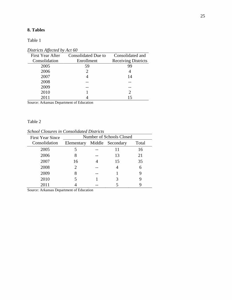
The results of this analysis are presented in Table 9. All specifications indicate a negative
impact of consolidation related school closure on student achievement; however the coefficient
estimates in the IV specifications are again much more negative than those in the OLS
specifications. Using the more specified models, we find that closure due to consolidation can be
expected to lead to performance declines of between 0.17 and 0.11 standard deviations in math
performance and between 0.5 and 1.0 standard deviations in literacy performance. Furthermore,
we note that the coefficient estimates on the control variables are largely unchanged, giving us
more confidence in our results.
[Table 9 here]
These larger, negative effects of school closure in the instrumental variable analysis
relative to the OLS analysis, suggest that the schools selected for closure contain students and
staff that have particular difficulty with transitions.
6. Conclusion
student
achiev
350 students.
Unfortunately, differences in what constitutes appropriate comparison groups does not allow us

20
to separately estimate the effects of consolidation on sending and receiving students in the same
model. In particular, students who were in consolidating districts are appropriately compared
against other students in small districts, while receiving districts are often quite large, requiring
an expanded control group.
among consolidated st -
It should b
-
discontin R -
-
the one just belo
R our
instrumental variable models for all students affected by consol
school closure induced by
consolidation give us some reason to
worried about the effects of district and school scale on student achievement. Even in very

21
small distr
organizations, they ar
Finally, we should note some potential issues with our paper. First, it is important to note
that our analysis treats all consolidations as homogenous, rather than heterogeneous, events. This
is largely because our paper offers an analysis of the effect of a statewide mandatory
consolidation policy rather than a study of individual district mergers. Nevertheless, we note that
the evidence presented in this paper largely focuses on the average effect of consolidation on
different types of students; and that these effects may certainly differ across district mergers.
In addition, preliminary reviewers of this paper raised the concern that districts may have
manipulated their enrollment to avoid consolidation. If this occurred on a large scale the effect
estimates presented in this paper would be biased. Nevertheless, there is little evidence that this
occurred in Arkansas. Furthermore, we note that the majority of districts subject to Act 60
consolidated during the first summer after the passage of the law; and therefore had no chance to
manipulate their enrollment. Thus, this concern, while valid, is unlikely to have had a strong
impact on the findings presented in this paper.
Finally, it is poss

22
improvements in

23
7. References
Alesina, A., Baqir, R., & Hoxby, C. (2004). Political Jurisdictions in Heterogeneous
Communities. Journal of Political Economy, 112(2), 348-396.
Andrews, M., Duncombe, W., & Yinger, J. (2002). Revisiting Economies of Size in American
Education: Are We Any Closer to a Consensus? Economics of Education Review, 21,
245-262.
84 “ 6 ” R ved
from http://www.arkleg.state.ar.us.
Arkansas Department of Education. (2006). Rule Governing the Consolidation or Annexation of
Public School Districts and Boards of Directors of Local School Districts. Retrieved from
http://www.arkansased.org.
Arkansas Bureau of Legislative Research. (2006). Educating Rural Arkansas: Issues of Declining
Enrollment, Isolated Schools, and High-Poverty Districts. Research Project 06-137
(August 2006). Prepared for the Adequacy Study Oversight Subcommittee of the
Arkansas Senate and House Committees on Education.
Barnett, J.H., Ritter, G.W., & Lucas, C.J. (2002). Educational Reform in Arkansas: Making
Sense of the Debate over School Consolidation. Arkansas Education Research & Policy
Studies Journal. 2 (2), 1-21.
Brasington, D. M. (2003). Size and School District Effects: Do Opposites Attract? Economica,
70(280), 673-690.
Berry, C.R. & West, M.R. (2008). Growing Pains: The School Consolidation Movement and
Student Outcomes. The Journal of Law, Economics, & Organization, 26(1).
Duncombe, W. & Yinger, J. (2007). Does School District Consolidation Cut Costs? Education
Finance and Policy. 2(4), 341-375.
Gordon, N. & Knight, B. (2006). The Causes of Political Integration: An Application to School
Districts. NBER Working Paper No 12047.
Hu, Y. & Yinger, J. (2007). The Impact of School District Consolidation on Housing Prices.
Unpublished Paper, Syracuse University.
Leithwood, K. & Jantzi, D. (2009). A Review of Empirical Evidence About School Size Effects:
A Policy Perspective. Review of Educational Research. 79(1), 464-490.

24
Kuziemko, I. (2006). Using Shocks to School Enrollment to Estimate the Effect of School Size
on Student Achievement. Economics of Education Review, 25, 63-75.
Nitta, K.A., Holley, M. J., & Wrobel, S. L. (2010). A Phenomenological Study of Rural School
Consolidation. Journal of Research in Rural Education, 25(2), 1-19. Retrieved from
http://www.jrre.psu.edu/articles/25-2.pdf.
Staiger, D. & Stock, J. H. (1997). Instrumental Variables Regression with Weak Instruments.
Econometrica, 65, pp. 557 – 586.
Walberg, H.J. & Fowler, W.J. (1987). Expenditure and Size Efficiencies of Public School
Districts. Educational Researcher, 16(7), pp. 5-13.
25
8. Tables
Table 1
Districts Affected by Act 60
First Year After
Consolidation
Consolidated Due to
Enrollment
Consolidated and
Receiving Districts
2005 59 99
2006 2 4
2007 4 14
2008 -- --
2009 -- --
2010 1 2
2011 4 15 Source: Arkansas Department of Education
Table 2
School Closures in Consolidated Districts
First Year Since
Consolidation
Number of Schools Closed
Elementary Middle Secondary Total
2005 5 -- 11 16
2006 8 -- 13 21
2007 16 4 15 35
2008 2 -- 4 6
2009 8 -- 1 9
2010 5 1 3 9
2011 4 -- 5 9 Source: Arkansas Department of Education

26
Table 3
Demographic Distributions for RD Models
OLS Regressions Student Fixed Effects
Control Treatment Control Treatment
N % N % N % N %
Total 23,276 --- 5,248 --- 23,331 --- 5,259 ---
Ethnicity
White 18,572 79.8 3,948 75.2 18,575 79.6 3,952 75.1
African American 3,197 13.7 1,131 21.6 3,199 13.7 1,133 21.5
Hispanic 513 2.2 59 1.1 513 2.2 59 1.1
Other 994 4.3 110 2.1 1,002 4.3 111 2.1
Gender
Male 11,902 51.1 2,578 49.1 11,902 51.0 2,578 49.0
Female 11,374 48.9 2,670 50.9 11,374 48.8 2,670 50.8
FRL Eligible 14,599 62.7 3,546 67.6 14,605 62.6 3,549 67.5
ELL 163 0.7 10 0.2 163 0.7 10 0.2
School Year
2003-04 30 0.1 0 0.0 30 0.1 0 0.0
2004-05 1,707 7.3 936 17.8 1,709 7.3 936 17.8
2005-06 4,131 17.7 1,434 27.3 4,138 17.7 1,440 27.4
2006-07 3,641 15.6 1,270 24.2 3,644 15.6 1,271 24.2
2007-08 3,638 15.6 774 14.7 3,638 15.6 774 14.7
2008-09 3,615 15.5 270 5.1 3,616 15.5 270 5.1
2009-10 3,519 15.1 193 3.7 3,546 15.2 196 3.7
2010-11 2,995 12.9 371 7.1 3,010 12.9 372 7.1 Notes: Differences-in-means tests are significant in all cases; however this is largely due to the large samples
available for comparison. Initial analyses confirm that these tests have sufficient power to detect differences as small
as those presented in this table.

27
Table 4
OLS Regressions, Preferred Enrollment Band of 250-450
Mathematics Literacy
Variable (1) (2) (3) (4)
Consolidated 0.017* 0.030*** 0.030*** 0.040***
(0.010) (0.010) (0.009) (0.009)
Lagged district average
enrollment -0.000 -0.000 -0.000** -0.000**
(0.000) (0.000) (0.000) (0.000)
Squared Lagged district
average enrollment 0.000 0.000 0.000 0.000
(0.000) (0.000) (0.000) (0.000)
Cubed Lagged district
average enrollment -0.000 -0.000 -0.000 -0.000
(0.000) (0.000) (0.000) (0.000)
Lagged performance 0.775*** 0.753*** 0.822*** 0.792***
(0.006) (0.006) (0.004) (0.005)
Female 0.035*** 0.106***
(0.006) (0.006)
Hispanic 0.052** 0.071***
(0.027) (0.022)
African American -0.078* -0.084***
(0.009) (0.009)
Other, non-white -0.005 0.009
(0.018) (0.017)
Free- or Reduced-Lunch
eligible -0.106*** -0.091***
(0.007) (0.007)
English Language
Learner -0.108** -0.063
(0.046) (0.046)
N 28,590 28524 28,586 28,520
Adjusted R-Squared 0.61 0.62 0.66 0.67 * denotes significance at the 10% level; ** denotes significance at the 5% level; *** denotes significance at the 1%
level
Notes: Standard errors are clustered at the student level. All specifications include Grade*Year controls.

28
Table 5
Years Since, OLS models only
Mathematics Literacy
Variable (1) (2) (3) (4)
One Year Since
Consolidation 0.009 0.023 0.041*** 0.053***
(0.016) (0.016) (0.016) (0.016)
Two Years Since
Consolidation 0.029 0.036* 0.002 0.008
(0.019) (0.019) (0.018) (0.018)
Three or More Years
Since Consolidation 0.017 0.033* 0.038** 0.052***
(0.017) (0.018) (0.016) (0.017)
Lagged district average
enrollment -0.000 -0.000 -0.000* -0.000*
(0.000) (0.000) (0.000) (0.000)
Squared Lagged district
average enrollment 0.000 0.000 0.000 0.000
(0.000) (0.000) (0.000) (0.000)
Cubed Lagged district
average enrollment -0.000 -0.000 -0.000 -0.000
(0.000) (0.000) (0.000) (0.000)
Lagged performance 0.775*** 0.753*** 0.822*** 0.792***
(0.006) (0.006) (0.004) (0.005)
Demographic Controls No Yes No Yes
N 28,590 28,524 28,586 28,520
Adjusted R-Squared 0.61 0.62 0.66 0.67 * denotes significance at the 10% level; ** denotes significance at the 5% level; *** denotes significance at the 1%
level
Notes: Standard errors are clustered at the student level. All specifications include Grade*Year controls.

29
Table 6
-
Mathematics Literacy
Variable (1) (2) (3) (4)
Consolidated 0.058*** 0.036*
(0.022) (0.022)
One Year Since
Consolidation 0.058** 0.042*
(0.022) (0.022)
Two Years Since
Consolidation 0.067** 0.017
(0.028) (0.028)
Three or More Years
Since Consolidation 0.144*** 0.091***
(0.031) (0.030)
Lagged district average
enrollment 0.000*** 0.000*** 0.000*** 0.000**
(0.000) (0.000) (0.000) (0.000)
Squared Lagged district
average enrollment -0.000*** -0.000** -0.000** -0.000**
(0.000) (0.000) (0.000) (0.000)
Cubed Lagged district
average enrollment 0.000*** 0.000* 0.000** 0.000*
(0.000) (0.000) (0.000) (0.000)
N 28,590 28,590 28,586 28,586 * denotes significance at the 10% level; ** denotes significance at the 5% level; *** denotes significance at the 1%
level
Notes: All specifications include Grade*Year controls.

30
Table 7
Specification Checks, OLS models
Mathematics Literacy
300-400 275-425
Less than
700 300-400 275-425
Less than
700
Variable (1) (2) (3) (4) (5) (6)
Consolidated 0.022* 0.022* 0.007 0.050*** 0.039*** 0.016**
(0.013) (0.011) (0.007) (0.012) (0.010) (0.006)
Lagged district average
enrollment
0.000 -0.000 -0.000 -0.000* -0.000* -0.000*
(0.000) (0.000) (0.000) (0.000) (0.000) (0.000)
Squared Lagged district
average enrollment
-0.000 0.000 -0.000 0.000 0.000 0.000
(0.000) (0.000) (0.000) (0.000) (0.000) (0.000)
Cubed Lagged district
average enrollment
-0.000 -0.000 -0.000 -0.000 -0.000 -0.000
(0.000) (0.000) (0.000) (0.000) (0.000) (0.000)
Lagged performance 0.755*** 0.757*** 0.758*** 0.795*** 0.791*** 0.798***
(0.009) (0.007) (0.003) (0.006) (0.005) (0.002)
Female 0.029*** 0.031*** 0.037*** 0.102*** 0.108*** 0.11***
(0.009) (0.007) (0.003) (0.008) (0.007) (0.003)
Hispanic 0.100** 0.054 0.038*** 0.095*** 0.072 0.031***
(0.051) (0.036) (0.011) (0.036) (0.028) (0.010)
African American -0.080*** -0.074*** -0.119*** -0.082*** -0.08*** -0.106***
(0.012) (0.010) (0.005) (0.011) (0.010) (0.005)
Other, non-white -0.039* -0.03 0.012 -0.005 0.006 0.012
(0.023) (0.021) (0.010) (0.022) (0.020) (0.009)
Free- or Reduced-
Lunch eligible
-0.119*** -0.117*** -0.09*** -0.089*** -0.094*** -0.078***
(0.010) (0.008) (0.004) (0.009) (0.007) (0.003)
English Language
Learner
-0.298*** -0.235*** -0.078*** -0.193 -0.197*** -0.049***
(0.093) (0.074) (0.017) (0.101) (0.073) (0.017)
N 15,400 21,633 108,078 15,399 21,632 108,052
Adjusted R-Squared 0.62 0.62 0.62 0.67 0.67 0.68 * denotes significance at the 10% level; ** denotes significance at the 5% level; *** denotes significance at the 1% level
Notes: Standard errors are clustered at the student level. All specifications include Grade*Year controls.

31
Table 8
Estimated Impacts of Consolidation on Receiving District Student Achievement
Mathematics Literacy
OLS 2SLS OLS 2SLS
Variable (1) (2) (3) (4) (5) (6) (7) (8)
In Receiving District 0.006*** 0.011*** -0.153*** -0.118*** 0.003* 0.007*** -0.113*** -0.066***
(0.002) (0.002) (0.006) (0.006) (0.002) (0.002) (0.005) (0.005)
Lagged performance 0.800*** 0.763*** 0.800*** 0.763*** 0.816*** 0.778*** 0.816*** 0.777***
(0.001) (0.001) (0.001) (0.001) (0.001) (0.001) (0.001) (0.001)
Female 0.023*** 0.023*** 0.096*** 0.096***
(0.001) (0.001) (0.001) (0.001)
Hispanic 0.032*** 0.028*** 0.041*** 0.038***
(0.003) (0.003) (0.003) (0.003)
African American -0.13*** -0.131*** -0.105*** -0.106***
(0.001) (0.002) (0.001) (0.001)
Other, non-white 0.027*** 0.021*** 0.022*** 0.019***
(0.003) (0.003) (0.003) (0.003)
Free- or Reduced-
Lunch eligible -0.126*** -0.124*** -0.11*** -0.109***
(0.001) (0.001) (0.001) (0.001)
English Language
Learner -0.065*** -0.067*** -0.032*** -0.033***
(0.003) (0.004) (0.003) (0.003)
N 1,038,939 1,030,269 1,038,939 1,030,269 1,038,715 1,030,053 1,038,715 1,030,053
Adjusted R-Squared 0.64 0.64 0.63 0.64 0.67 0.68 0.67 0.68 * denotes significance at the 10% level; ** denotes significance at the 5% level; *** denotes significance at the 1% level
Notes: Robust standard errors presented in parentheses. First stage regressions indicate a significant negative relationship between the consolidation instrument
and school closure equal to -0.010 across all specifications. This confirms our expectations about the instrumental variable: districts are significantly more likely
to be identified as receiving districts if they are in close proximity to a consolidated district. First stage F-statistics range from 682.7 to 770.6, which are
substantially higher than acceptable threshold recommended by Staiger and Stock (1997) of 10.
32
Table 9
Estimated Impacts of School Closure due to Consolidation
Mathematics Literacy
OLS 2SLS OLS 2SLS
Variable (1) (2) (3) (4) (5) (6) (7) (8)
Closure affected -0.062*** -0.020*** -0.174*** -0.115*** -0.057*** -0.025*** -0.100*** -0.054***
(0.005) (0.006) (0.020) (0.021) (0.005) (0.005) (0.019) (0.020)
Lagged performance 0.800*** 0.763*** 0.800*** 0.763*** 0.816*** 0.778*** 0.816*** 0.778***
(0.001) (0.001) (0.001) (0.001) (0.001) (0.001) (0.001) (0.001)
Female
0.023*** 0.023***
0.096*** 0.096***
(0.001) (0.001)
(0.001) (0.001)
Hispanic
0.032*** 0.031***
0.041*** 0.04***
(0.003) (0.003)
(0.003) (0.003)
African American
-0.130*** -0.129***
-0.105*** -0.105***
(0.001) (0.002)
(0.001) (0.001)
Other, non-white
0.026*** 0.026***
0.021*** 0.021***
(0.003) (0.003)
(0.003) (0.003)
Free- or Reduced-Lunch
eligible
-0.126*** -0.125***
-0.109*** -0.109***
(0.001) (0.001)
(0.001) (0.001)
English Language
Learner
-0.065*** -0.066***
-0.032*** -0.032***
(0.003) (0.003)
(0.003) (0.003)
N 1,038,939 1,030,269 1,038,939 1,030,269 1,038,715 1,030,053 1,038,715 1,030,053
Adjusted R-Squared 0.63 0.64 0.63 0.64 0.67 0.68 0.67 0.68 * denotes significance at the 10% level; ** denotes significance at the 5% level; *** denotes significance at the 1% level
Notes: Robust standard errors presented in parentheses. First stage regressions indicate a significant relationship between the consolidation instrument and school
closure equal to roughly 0.29 across all specifications. This indicates that schools in districts subject to Act 60 are significantly more likely to be closed, as
expected. First stage F-statistics range from 70.6 to 84.3, which are substantially higher than acceptable threshold recommended by Staiger and Stock (1997) of
10.