An Analysis of the Stability of Deep Drilling Systems

A DISSERTATION

SUBMITTED TO THE FACULTY OF THE GRADUATE SCHOOL

OF THE UNIVERSITY OF MINNESOTA

BY

Carlos Eduardo da Fonseca

IN PARTIAL FULFILLMENT OF THE REQUIREMENTS

FOR THE DEGREE OF

MASTER OF SCIENCE

ADVISER

Emmanuel Detournay

CO-ADVISER

Nathan van de Wouw

July, 2015

c© Carlos Eduardo da Fonseca 2015

ALL RIGHTS RESERVED

Acknowledgements

First of all, I want to express my sincere gratitude to Petróleo Brasileiro S.A - Petrobras,

which supported in many ways my travel to the Minneapolis, and my time at the University of

Minnesota.

My sincere thanks to my adviser Prof. Emmanuel Detournay for the continuous support,

patience, and understanding about everything that had happened during these two years. Also,

my sincere thanks to my co-adviser Prof. Nathan van de Wouw, who was always ready to teach

and help.

Also I have to thanks my new friends. Anna Liakou, who helped me a lot during my rst

semester as a student, and throughout my entire journey. To Julien Marck, for the uncountable

number of great discussions we had. To Yaneng Zhou, who always inspired me to be a nicer

person. And Kaixao Tian, who joined us recently, and has been a wonderful person.

I can not forget about the great number of people who I met and helped me to make the

Minnesota weather more enjoyable. Even though their names are not listed here, they will

always be part of my memories and my life. And last but not least, my family and friends in

Brazil, who has been supporting and waiting for us.

i

Dedication

I dedicate my dissertation to my family, who accepted the challenge to change to a completely

new life. My wife Fabiana, who came with the compromise of bringing our new baby to us.

Gabriel, who had no idea what was about to come, and enjoyed it a lot. And Julia, who just

arrived within this time in Minneapolis.

My family dedicate this journey to my dad, José Geraldo, who left before we came to

Minneapolis.

Also my family dedicate this work to Regina, who left before we went back to Rio de Janeiro.

ii

Abstract

This thesis has focused on analyzing the coupled axial-torsional dynamics of a drilling structure,

due to its importance within the drilling activity. This work builds upon earlier published work

on the coupled axial-torsional dynamics of drilling systems, which addressed the problem by

means of either low-order or nite element models. During the course of this study we realized

that the spatial discrete representation of the drilling system plays an important role in the model

stability properties; in particular the model tends to become more unstable when it is represented

by a larger number of DOF's (i.e. a ner discretization). Ultimately, such a lack of stability can

be an inherent property of the drilling system. If the observed instability of the drilling system

is indeed an inherent property, only signicant changes to the dynamics can provide system

stability. Focusing on that aspect, a nite element model was used to investigate the value of

the use of a simple (industrial) angular velocity drive system control (Soft Torque) to mitigate

stick-slip. The Soft Torque controller can be represented by a spring-dash pot surface boundary

condition which is tuned to damp the rst torsional natural frequency of the drill string. From

the results in the thesis, it can be concluded that the coupled axial-torsional dynamics, with the

bit/rock interface, cannot in general be stabilized by the Soft Torque controller. This is likely to

be related to the fact that higher modes of the drill-string dynamics play a role in instabilities

leading to stick-slip oscillations. Motivated by this observation, this study took on the challenge

of investigating which level of discretization provides and accurate description in the dynamics.

To understand the role of spatial discretization of the drill-string dynamics, discrete models

were developed to understand stability properties and to study the overall time-domain behavior.

Based on a time scale separation argument (between the axial and torsional dynamics), 1-DOF,

2-DOF, and multi-DOF lumped parameter models describing only the axial dynamics of the drill-

string were studied. Subsequently, the coupled dynamics of one and two identical oscillators were

investigated. In all cases, the increasing number of oscillators led to a more unstable system.

iii

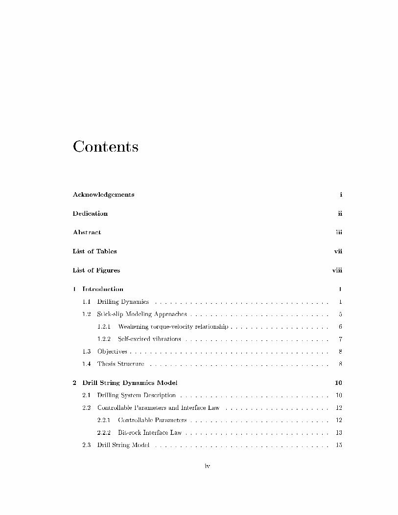
Contents

Acknowledgements i

Dedication ii

Abstract iii

List of Tables vii

List of Figures viii

1 Introduction 1

1.1 Drilling Dynamics . . . . . . . . . . . . . . . . . . . . . . . . . . . . . . . . . . . 1

1.2 Stick-slip Modeling Approaches . . . . . . . . . . . . . . . . . . . . . . . . . . . . 5

1.2.1 Weakening torque-velocity relationship . . . . . . . . . . . . . . . . . . . . 6

1.2.2 Self-excited vibrations . . . . . . . . . . . . . . . . . . . . . . . . . . . . . 7

1.3 Objectives . . . . . . . . . . . . . . . . . . . . . . . . . . . . . . . . . . . . . . . . 8

1.4 Thesis Structure . . . . . . . . . . . . . . . . . . . . . . . . . . . . . . . . . . . . 8

2 Drill String Dynamics Model 10

2.1 Drilling System Description . . . . . . . . . . . . . . . . . . . . . . . . . . . . . . 10

2.2 Controllable Parameters and Interface Law . . . . . . . . . . . . . . . . . . . . . 12

2.2.1 Controllable Parameters . . . . . . . . . . . . . . . . . . . . . . . . . . . . 12

2.2.2 Bit-rock Interface Law . . . . . . . . . . . . . . . . . . . . . . . . . . . . . 13

2.3 Drill String Model . . . . . . . . . . . . . . . . . . . . . . . . . . . . . . . . . . . 15

iv

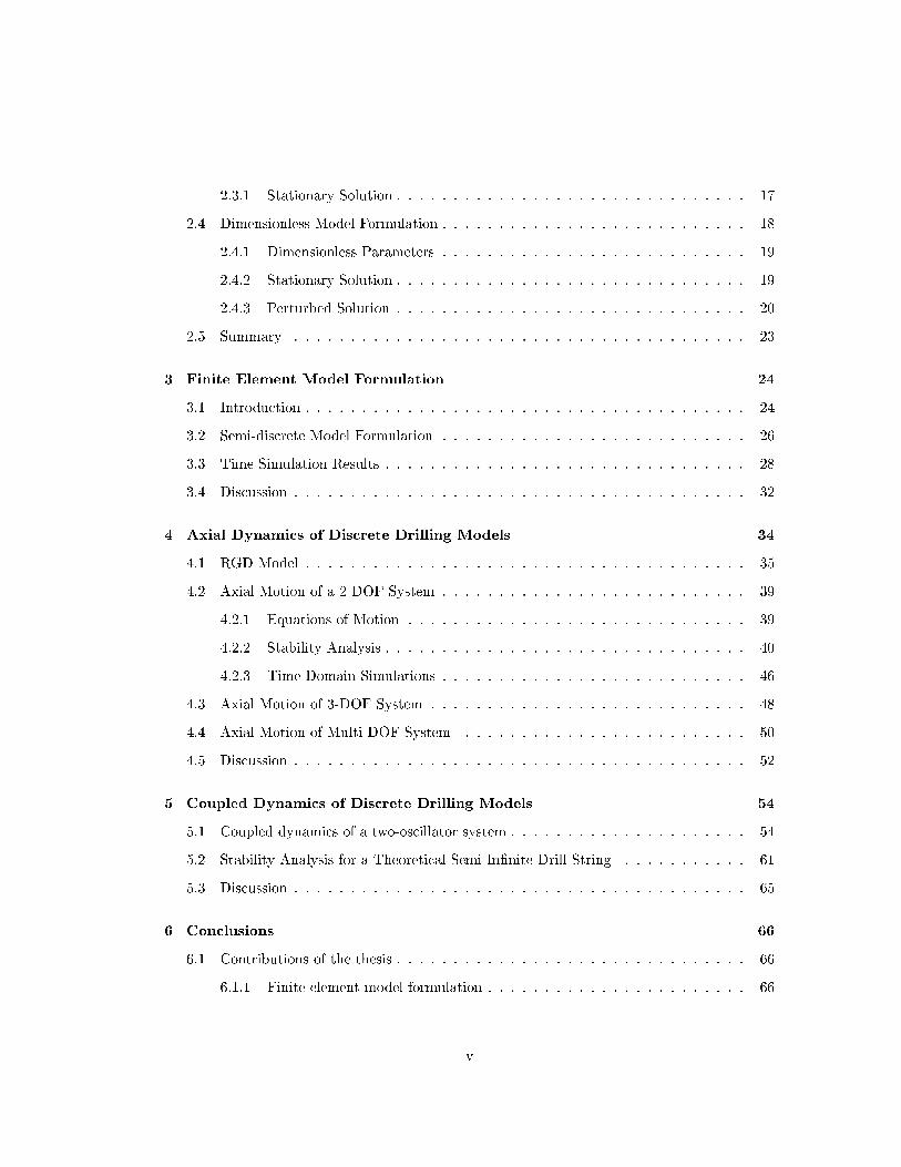
2.3.1 Stationary Solution . . . . . . . . . . . . . . . . . . . . . . . . . . . . . . . 17

2.4 Dimensionless Model Formulation . . . . . . . . . . . . . . . . . . . . . . . . . . . 18

2.4.1 Dimensionless Parameters . . . . . . . . . . . . . . . . . . . . . . . . . . . 19

2.4.2 Stationary Solution . . . . . . . . . . . . . . . . . . . . . . . . . . . . . . . 19

2.4.3 Perturbed Solution . . . . . . . . . . . . . . . . . . . . . . . . . . . . . . . 20

2.5 Summary . . . . . . . . . . . . . . . . . . . . . . . . . . . . . . . . . . . . . . . . 23

3 Finite Element Model Formulation 24

3.1 Introduction . . . . . . . . . . . . . . . . . . . . . . . . . . . . . . . . . . . . . . . 24

3.2 Semi-discrete Model Formulation . . . . . . . . . . . . . . . . . . . . . . . . . . . 26

3.3 Time Simulation Results . . . . . . . . . . . . . . . . . . . . . . . . . . . . . . . . 28

3.4 Discussion . . . . . . . . . . . . . . . . . . . . . . . . . . . . . . . . . . . . . . . . 32

4 Axial Dynamics of Discrete Drilling Models 34

4.1 RGD Model . . . . . . . . . . . . . . . . . . . . . . . . . . . . . . . . . . . . . . . 35

4.2 Axial Motion of a 2 DOF System . . . . . . . . . . . . . . . . . . . . . . . . . . . 39

4.2.1 Equations of Motion . . . . . . . . . . . . . . . . . . . . . . . . . . . . . . 39

4.2.2 Stability Analysis . . . . . . . . . . . . . . . . . . . . . . . . . . . . . . . . 40

4.2.3 Time-Domain Simulations . . . . . . . . . . . . . . . . . . . . . . . . . . . 46

4.3 Axial Motion of 3-DOF System . . . . . . . . . . . . . . . . . . . . . . . . . . . . 48

4.4 Axial Motion of Multi-DOF System . . . . . . . . . . . . . . . . . . . . . . . . . 50

4.5 Discussion . . . . . . . . . . . . . . . . . . . . . . . . . . . . . . . . . . . . . . . . 52

5 Coupled Dynamics of Discrete Drilling Models 54

5.1 Coupled dynamics of a two-oscillator system . . . . . . . . . . . . . . . . . . . . . 54

5.2 Stability Analysis for a Theoretical Semi-Innite Drill String . . . . . . . . . . . 61

5.3 Discussion . . . . . . . . . . . . . . . . . . . . . . . . . . . . . . . . . . . . . . . . 65

6 Conclusions 66

6.1 Contributions of the thesis . . . . . . . . . . . . . . . . . . . . . . . . . . . . . . . 66

6.1.1 Finite element model formulation . . . . . . . . . . . . . . . . . . . . . . . 66

v

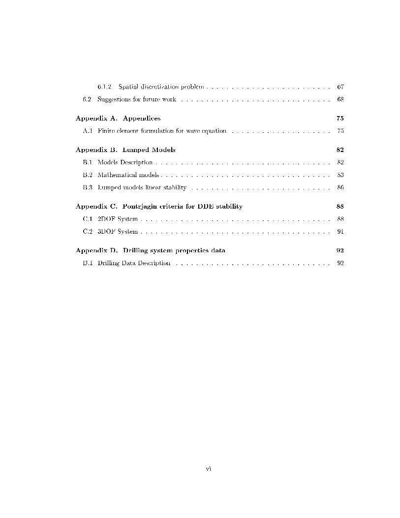
6.1.2 Spatial discretization problem . . . . . . . . . . . . . . . . . . . . . . . . . 67

6.2 Suggestions for future work . . . . . . . . . . . . . . . . . . . . . . . . . . . . . . 68

Appendix A. Appendices 75

A.1 Finite element formulation for wave equation . . . . . . . . . . . . . . . . . . . . 75

Appendix B. Lumped Models 82

B.1 Models Description . . . . . . . . . . . . . . . . . . . . . . . . . . . . . . . . . . . 82

B.2 Mathematical models . . . . . . . . . . . . . . . . . . . . . . . . . . . . . . . . . . 83

B.3 Lumped models linear stability . . . . . . . . . . . . . . . . . . . . . . . . . . . . 86

Appendix C. Pontrjagin criteria for DDE stability 88

C.1 2DOF System . . . . . . . . . . . . . . . . . . . . . . . . . . . . . . . . . . . . . . 88

C.2 3DOF System . . . . . . . . . . . . . . . . . . . . . . . . . . . . . . . . . . . . . . 91

Appendix D. Drilling system properties data 92

D.1 Drilling Data Description . . . . . . . . . . . . . . . . . . . . . . . . . . . . . . . 92

vi

List of Tables

D.1.1Drilling system properties used within this thesis. . . . . . . . . . . . . . . . . . . 93

vii

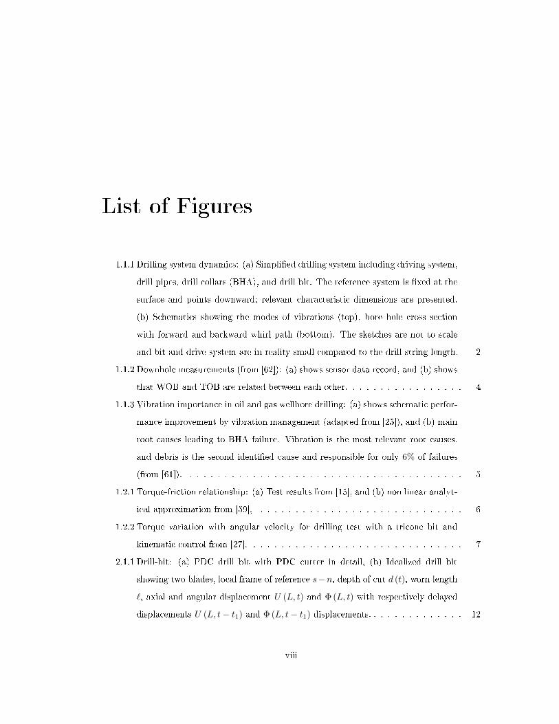
List of Figures

1.1.1 Drilling system dynamics: (a) Simplied drilling system including driving system,

drill pipes, drill collars (BHA), and drill bit. The reference system is xed at the

surface and points downward; relevant characteristic dimensions are presented.

(b) Schematics showing the modes of vibrations (top), bore hole cross section

with forward and backward whirl path (bottom). The sketches are not to scale

and bit and drive system are in reality small compared to the drill string length. 2

1.1.2 Downhole measurements (from [62]): (a) shows sensor data record, and (b) shows

that WOB and TOB are related between each other. . . . . . . . . . . . . . . . . 4

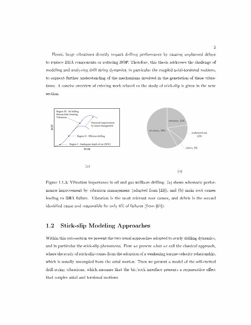
1.1.3 Vibration importance in oil and gas wellbore drilling: (a) shows schematic perfor-

mance improvement by vibration management (adapted from [25]), and (b) main

root causes leading to BHA failure. Vibration is the most relevant root causes,

and debris is the second identied cause and responsible for only 6% of failures

(from [61]). . . . . . . . . . . . . . . . . . . . . . . . . . . . . . . . . . . . . . . . 5

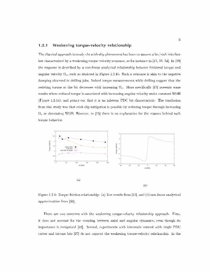
1.2.1 Torque-friction relationship: (a) Test results from [15], and (b) non linear analyt-

ical approximation from [59], . . . . . . . . . . . . . . . . . . . . . . . . . . . . . 6

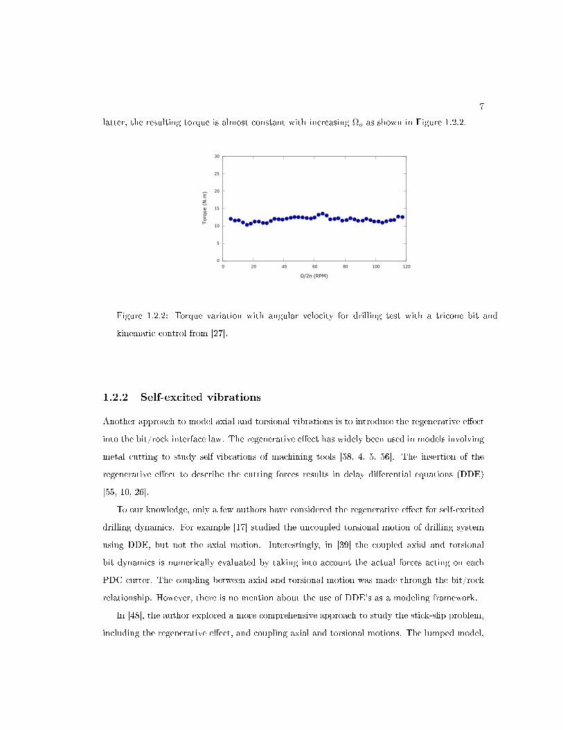
1.2.2 Torque variation with angular velocity for drilling test with a tricone bit and

kinematic control from [27]. . . . . . . . . . . . . . . . . . . . . . . . . . . . . . . 7

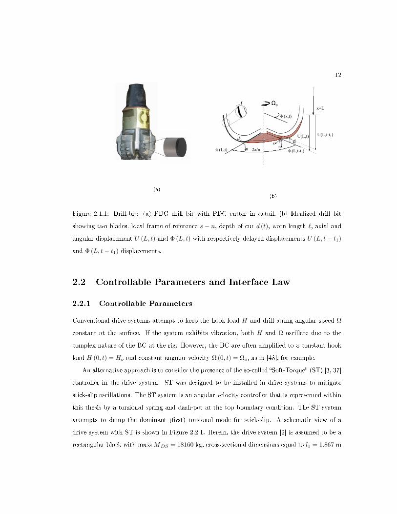
2.1.1 Drill-bit: (a) PDC drill bit with PDC cutter in detail, (b) Idealized drill bit

showing two blades, local frame of reference s−n, depth of cut d (t), worn length

`, axial and angular displacement U (L, t) and Φ (L, t) with respectively delayed

displacements U (L, t− t1) and Φ (L, t− t1) displacements. . . . . . . . . . . . . . 12

viii

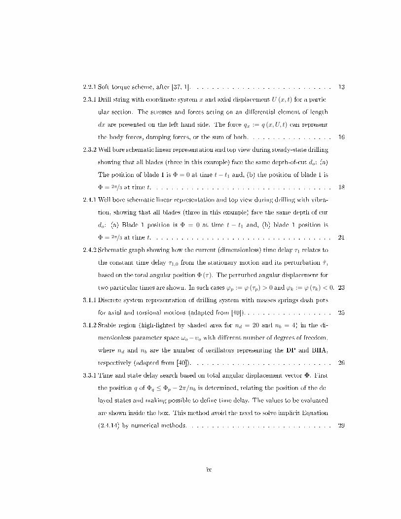
2.2.1 Soft torque scheme, after [37, 1]. . . . . . . . . . . . . . . . . . . . . . . . . . . . 13

2.3.1 Drill string with coordinate system x and axial displacement U (x, t) for a partic-

ular section. The stresses and forces acting on an dierential element of length

dx are presented on the left hand side. The force qx := q (x, U, t) can represent

the body forces, damping forces, or the sum of both. . . . . . . . . . . . . . . . . 16

2.3.2 Well bore schematic linear representation and top view during steady-state drilling

showing that all blades (three in this example) face the same depth-of-cut do: (a)

The position of blade 1 is Φ = 0 at time t− t1 and, (b) the position of blade 1 is

Φ = 2π/3 at time t. . . . . . . . . . . . . . . . . . . . . . . . . . . . . . . . . . . . 18

2.4.1 Well bore schematic linear representation and top view during drilling with vibra-

tion, showing that all blades (three in this example) face the same depth-of-cut

do: (a) Blade 1 position is Φ = 0 at time t − t1 and, (b) blade 1 position is

Φ = 2π/3 at time t. . . . . . . . . . . . . . . . . . . . . . . . . . . . . . . . . . . . 21

2.4.2 Schematic graph showing how the current (dimensionless) time delay τ1 relates to

the constant time delay τ1,0 from the stationary motion and its perturbation τ ,

based on the total angular position Φ (τ). The perturbed angular displacement for

two particular times are shown. In such cases ϕp := ϕ (τp) > 0 and ϕk := ϕ (τk) < 0. 23

3.1.1 Discrete system representation of drilling system with masses-springs-dash pots

for axial and torsional motions (adapted from [40]). . . . . . . . . . . . . . . . . . 25

3.1.2 Stable region (high-lighted by shaded area for nd = 20 and nb = 4) in the di-

mensionless parameter space ωo−υo with dierent number of degrees of freedom,

where nd and nb are the number of oscillators representing the DP and BHA,

respectively (adapted from [40]). . . . . . . . . . . . . . . . . . . . . . . . . . . . 26

3.3.1 Time and state delay search based on total angular displacement vector Φ. First

the position q of Φq ≤ Φp − 2π/nb is determined, relating the position of the de-

layed states and making possible to dene time delay. The values to be evaluated

are shown inside the box. This method avoid the need to solve implicit Equation

(2.4.14) by numerical methods. . . . . . . . . . . . . . . . . . . . . . . . . . . . . 29

ix

3.3.2 Evolution of bit velocities. The dynamics evolves in three phases: (i) axial stick,

(ii) increasing angular oscillations, and (iii) angular stick-slip. Left vertical axis

shows axial velocity, and right one shows angular velocity. . . . . . . . . . . . . . 30

3.3.3 Bit velocities evolution with ST. The three phases are also presented here. Left

vertical axis shows axial velocity, and right one shows angular velocity. . . . . . 31

3.3.4 Search procedure method check for drill system without ST (τ ≤ 250) and with

ST. The delay state must satisfy Equation (2.4.14), with small residual. . . . . . 32

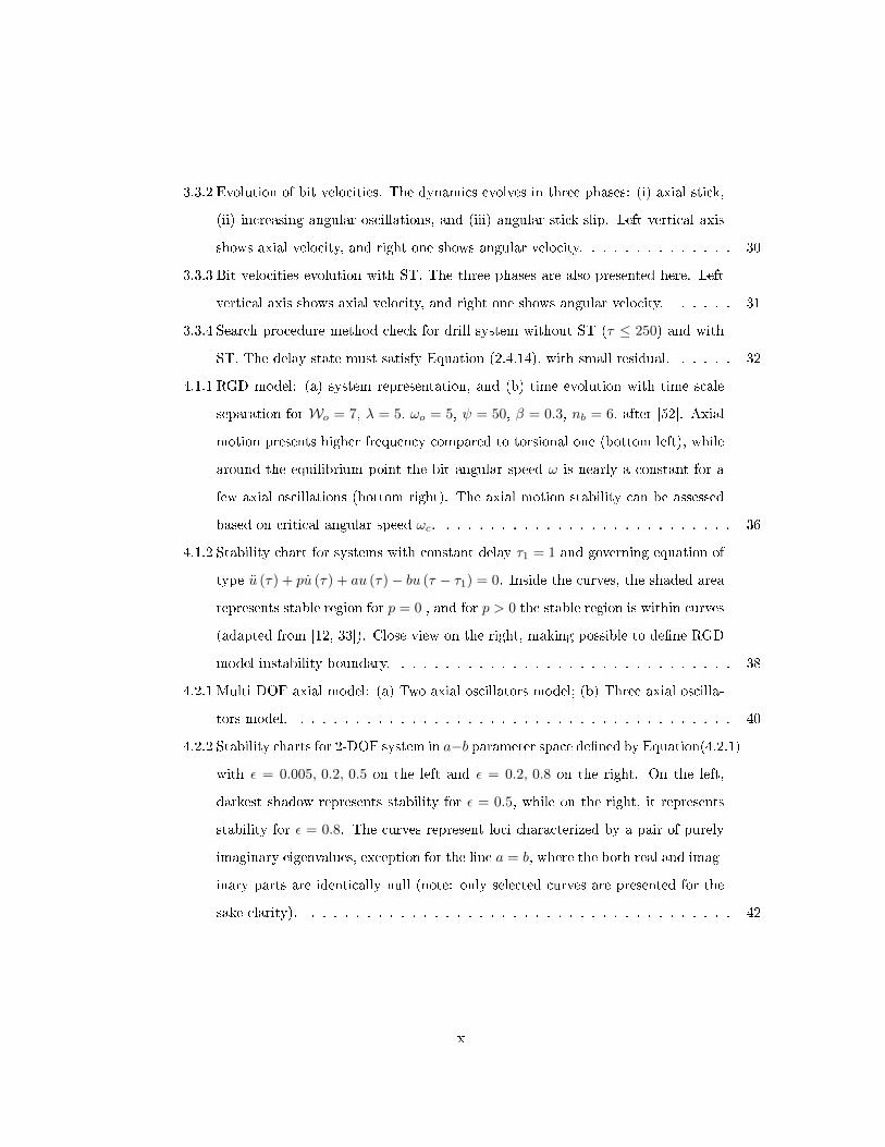
4.1.1 RGD model: (a) system representation, and (b) time evolution with time scale

separation for Wo = 7, λ = 5, ωo = 5, ψ = 50, β = 0.3, nb = 6, after [52]. Axial

motion presents higher frequency compared to torsional one (bottom left), while

around the equilibrium point the bit angular speed ω is nearly a constant for a

few axial oscillations (bottom right). The axial motion stability can be assessed

based on critical angular speed ωc. . . . . . . . . . . . . . . . . . . . . . . . . . . 36

4.1.2 Stability chart for systems with constant delay τ1 = 1 and governing equation of

type u (τ) + pu (τ) + au (τ)− bu (τ − τ1) = 0. Inside the curves, the shaded area

represents stable region for p = 0 , and for p > 0 the stable region is within curves

(adapted from [12, 33]). Close view on the right, making possible to dene RGD

model instability boundary. . . . . . . . . . . . . . . . . . . . . . . . . . . . . . . 38

4.2.1 Multi DOF axial model: (a) Two axial oscillators model; (b) Three axial oscilla-

tors model. . . . . . . . . . . . . . . . . . . . . . . . . . . . . . . . . . . . . . . . 40

4.2.2 Stability charts for 2-DOF system in a−b parameter space dened by Equation(4.2.1)

with ε = 0.005, 0.2, 0.5 on the left and ε = 0.2, 0.8 on the right. On the left,

darkest shadow represents stability for ε = 0.5, while on the right, it represents

stability for ε = 0.8. The curves represent loci characterized by a pair of purely

imaginary eigenvalues, exception for the line a = b, where the both real and imag-

inary parts are identically null (note: only selected curves are presented for the

sake clarity). . . . . . . . . . . . . . . . . . . . . . . . . . . . . . . . . . . . . . . 42

x

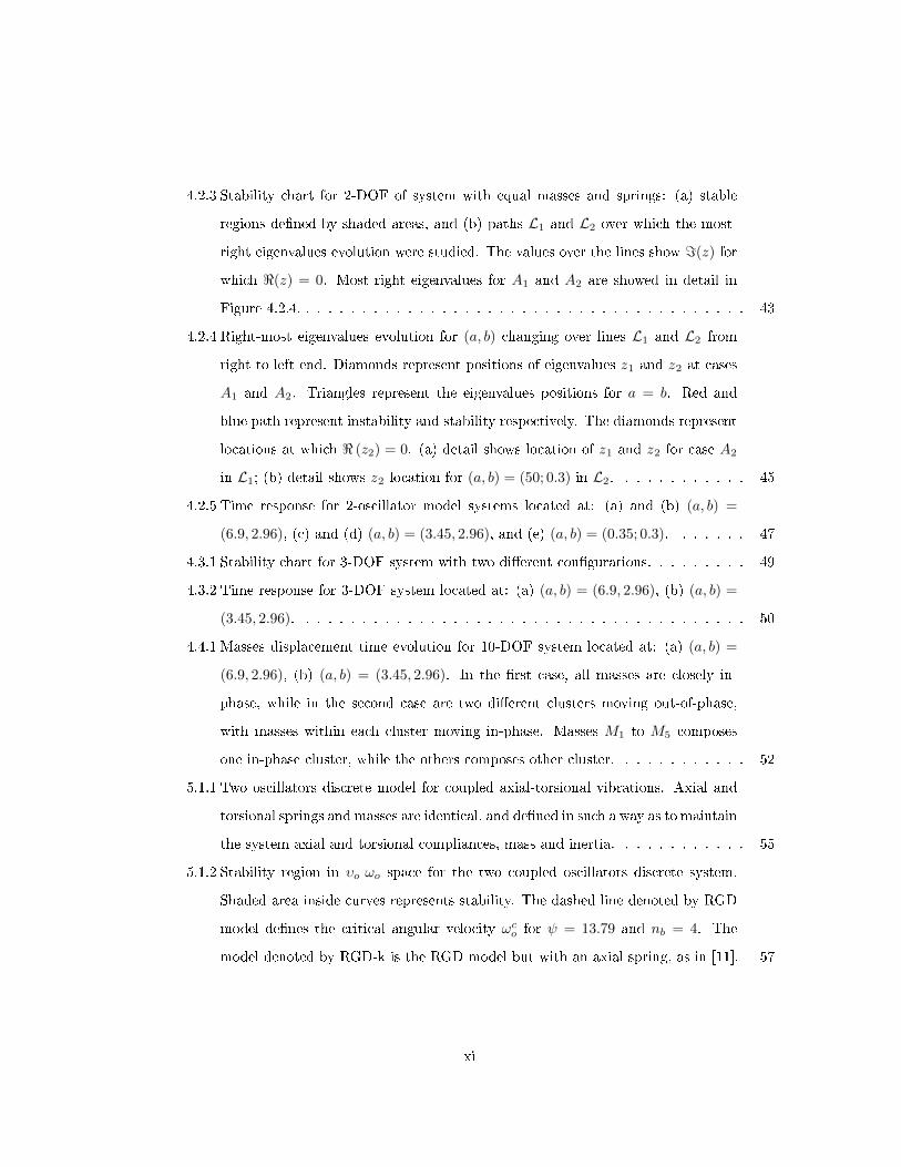
4.2.3 Stability chart for 2-DOF of system with equal masses and springs: (a) stable

regions dened by shaded areas, and (b) paths L1 and L2 over which the most-

right eigenvalues evolution were studied. The values over the lines show =(z) for

which <(z) = 0. Most right eigenvalues for A1 and A2 are showed in detail in

Figure 4.2.4. . . . . . . . . . . . . . . . . . . . . . . . . . . . . . . . . . . . . . . . 43

4.2.4 Right-most eigenvalues evolution for (a, b) changing over lines L1 and L2 from

right to left end. Diamonds represent positions of eigenvalues z1 and z2 at cases

A1 and A2. Triangles represent the eigenvalues positions for a = b. Red and

blue path represent instability and stability respectively. The diamonds represent

locations at which < (z2) = 0. (a) detail shows location of z1 and z2 for case A2

in L1; (b) detail shows z2 location for (a, b) = (50; 0.3) in L2. . . . . . . . . . . . 45

4.2.5 Time response for 2-oscillator model systems located at: (a) and (b) (a, b) =

(6.9, 2.96), (c) and (d) (a, b) = (3.45, 2.96), and (e) (a, b) = (0.35; 0.3). . . . . . . 47

4.3.1 Stability chart for 3-DOF system with two dierent congurations. . . . . . . . . 49

4.3.2 Time response for 3-DOF system located at: (a) (a, b) = (6.9, 2.96), (b) (a, b) =

(3.45, 2.96). . . . . . . . . . . . . . . . . . . . . . . . . . . . . . . . . . . . . . . . 50

4.4.1 Masses displacement time evolution for 10-DOF system located at: (a) (a, b) =

(6.9, 2.96), (b) (a, b) = (3.45, 2.96). In the rst case, all masses are closely in-

phase, while in the second case are two dierent clusters moving out-of-phase,

with masses within each cluster moving in-phase. Masses M1 to M5 composes

one in-phase cluster, while the others composes other cluster. . . . . . . . . . . . 52

5.1.1 Two oscillators discrete model for coupled axial-torsional vibrations. Axial and

torsional springs and masses are identical, and dened in such a way as to maintain

the system axial and torsional compliances, mass and inertia. . . . . . . . . . . . 55

5.1.2 Stability region in υo-ωo space for the two coupled oscillators discrete system.

Shaded area inside curves represents stability. The dashed line denoted by RGD

model denes the critical angular velocity ωco for ψ = 13.79 and nb = 4. The

model denoted by RGD-k is the RGD model but with an axial spring, as in [11]. 57

xi

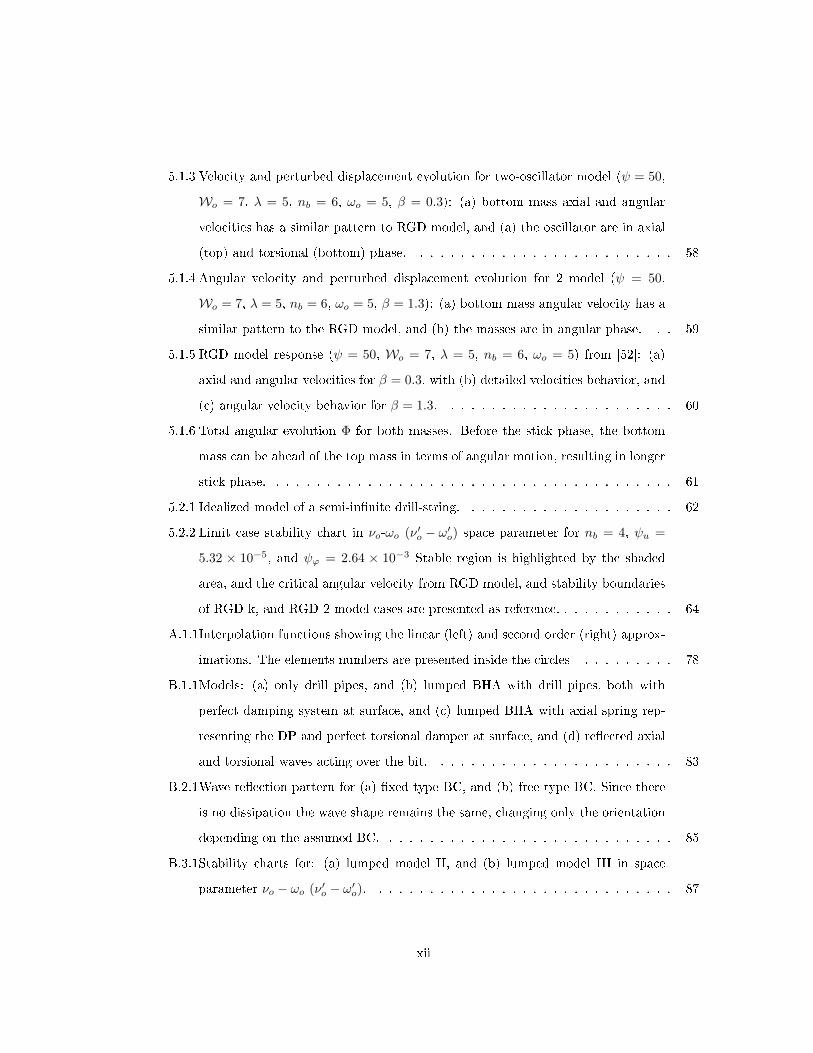
5.1.3 Velocity and perturbed displacement evolution for two-oscillator model (ψ = 50,

Wo = 7, λ = 5, nb = 6, ωo = 5, β = 0.3): (a) bottom mass axial and angular

velocities has a similar pattern to RGD model, and (a) the oscillator are in axial

(top) and torsional (bottom) phase. . . . . . . . . . . . . . . . . . . . . . . . . . 58

5.1.4 Angular velocity and perturbed displacement evolution for 2 model (ψ = 50,

Wo = 7, λ = 5, nb = 6, ωo = 5, β = 1.3): (a) bottom mass angular velocity has a

similar pattern to the RGD model, and (b) the masses are in angular phase. . . 59

5.1.5 RGD model response (ψ = 50, Wo = 7, λ = 5, nb = 6, ωo = 5) from [52]: (a)

axial and angular velocities for β = 0.3, with (b) detailed velocities behavior, and

(c) angular velocity behavior for β = 1.3. . . . . . . . . . . . . . . . . . . . . . . 60

5.1.6 Total angular evolution Φ for both masses. Before the stick phase, the bottom

mass can be ahead of the top mass in terms of angular motion, resulting in longer

stick phase. . . . . . . . . . . . . . . . . . . . . . . . . . . . . . . . . . . . . . . . 61

5.2.1 Idealized model of a semi-innite drill-string. . . . . . . . . . . . . . . . . . . . . 62

5.2.2 Limit case stability chart in νo-ωo (ν′o − ω′o) space parameter for nb = 4, ψu =

5.32 × 10−5, and ψϕ = 2.64 × 10−3 Stable region is highlighted by the shaded

area, and the critical angular velocity from RGD model, and stability boundaries

of RGD-k, and RGD-2 model cases are presented as reference. . . . . . . . . . . . 64

A.1.1Interpolation functions showing the linear (left) and second order (right) approx-

imations. The elements numbers are presented inside the circles . . . . . . . . . 78

B.1.1Models: (a) only drill pipes, and (b) lumped BHA with drill pipes, both with

perfect damping system at surface, and (c) lumped BHA with axial spring rep-

resenting the DP and perfect torsional damper at surface, and (d) reected axial

and torsional waves acting over the bit. . . . . . . . . . . . . . . . . . . . . . . . 83

B.2.1Wave reection pattern for (a) xed type BC, and (b) free type BC. Since there

is no dissipation the wave shape remains the same, changing only the orientation

depending on the assumed BC. . . . . . . . . . . . . . . . . . . . . . . . . . . . . 85

B.3.1Stability charts for: (a) lumped model II, and (b) lumped model III in space

parameter νo − ωo (ν′o − ω′o). . . . . . . . . . . . . . . . . . . . . . . . . . . . . . 87

xii

Chapter 1

Introduction

Wellbore construction is one the most expensive investment in oil and gas production, and thus

makes it an important activity throughout the exploitation chain. Construction of a wellbore

consists of three main tasks: (1) drilling (removing rock down to the hydrocarbon reservoir),

(2) casing (protecting the wellbore previously drilled with pipes), and (3) completion (installing

suitable equipment for hydrocarbon production control) [7, 13, 28].

To drill a well, the surface drive system imposes axial and angular velocities at the drill

pipe (DP) top end, which are transmitted to the bit. In the lower section of the drill string,

thicker pipes (drill collars) push the bit downward and are the main features in the bottom hole

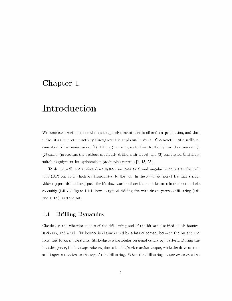
assembly (BHA). Figure 1.1.1 shows a typical drilling site with drive system, drill string (DP

and BHA), and the bit.

1.1 Drilling Dynamics

Classically, the vibration modes of the drill string and of the bit are classied as bit bounce,

stick-slip, and whirl. Bit bounce is characterized by a loss of contact between the bit and the

rock, due to axial vibrations. Stick-slip is a particular torsional oscillatory pattern. During the

bit stick phase, the bit stops rotating due to the bit/rock reaction torque, while the drive system

still imposes rotation to the top of the drill string. When the drill-string torque overcomes the

1

2

resisting bit/rock torque, the bit and drill string accelerate sharply in the slip phase leading

to high torsional velocity. Whirl is the out-of-center rotation of the bit and drill string due to

lateral vibrations; it can be forward or backward compared to the bit rotation orientation. The

three modes of vibrations are illustrated in Figure 1.1.1b.

(a)

(b)

Figure 1.1.1: Drilling system dynamics: (a) Simplied drilling system including driving system,

drill pipes, drill collars (BHA), and drill bit. The reference system is xed at the surface and

points downward; relevant characteristic dimensions are presented. (b) Schematics showing

the modes of vibrations (top), bore hole cross section with forward and backward whirl path

(bottom). The sketches are not to scale and bit and drive system are in reality small compared

to the drill string length.

The development of downhole data acquisition sensors has been the key to understand drilling

3

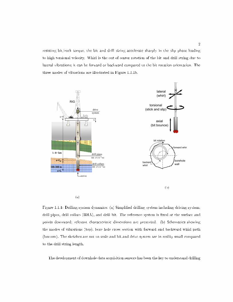
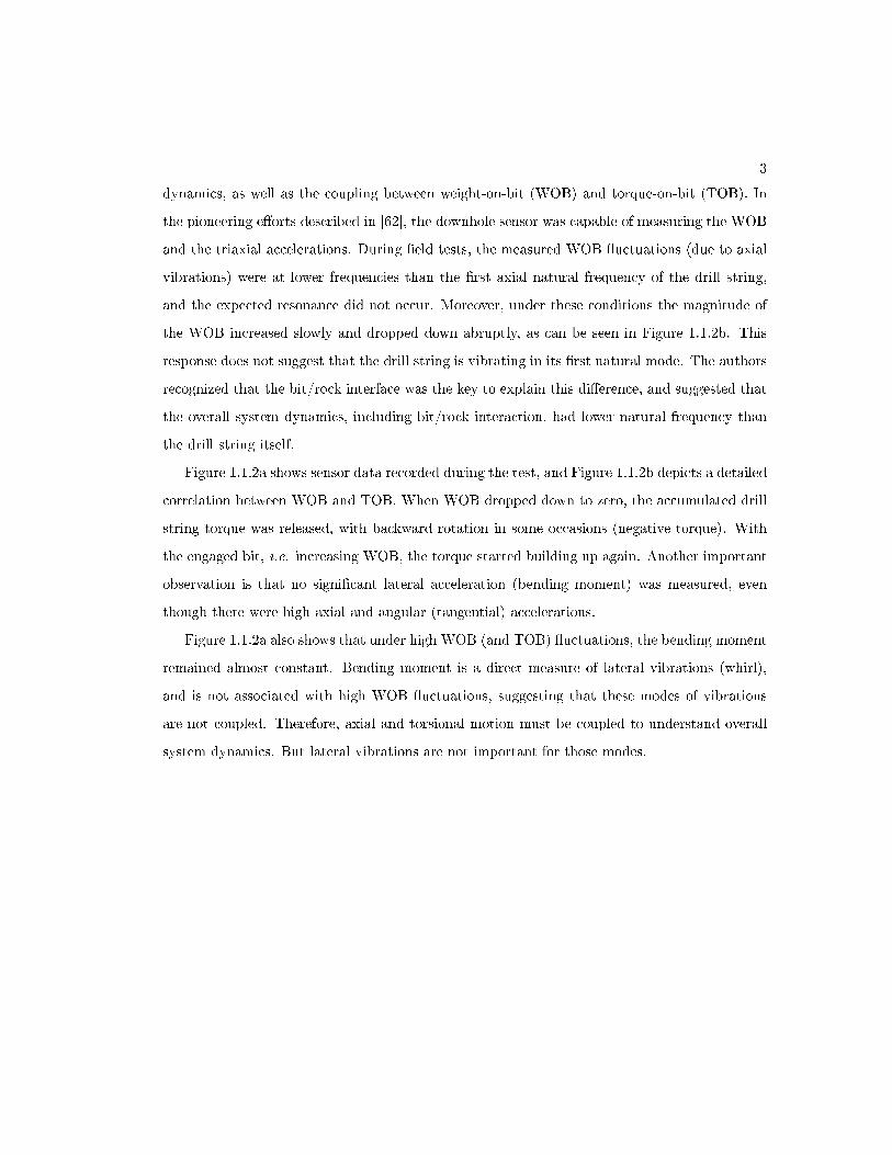
dynamics, as well as the coupling between weight-on-bit (WOB) and torque-on-bit (TOB). In

the pioneering eorts described in [62], the downhole sensor was capable of measuring the WOB

and the triaxial accelerations. During eld tests, the measured WOB uctuations (due to axial

vibrations) were at lower frequencies than the rst axial natural frequency of the drill string,

and the expected resonance did not occur. Moreover, under these conditions the magnitude of

the WOB increased slowly and dropped down abruptly, as can be seen in Figure 1.1.2b. This

response does not suggest that the drill string is vibrating in its rst natural mode. The authors

recognized that the bit/rock interface was the key to explain this dierence, and suggested that

the overall system dynamics, including bit/rock interaction, had lower natural frequency than

the drill string itself.

Figure 1.1.2a shows sensor data recorded during the test, and Figure 1.1.2b depicts a detailed

correlation between WOB and TOB. When WOB dropped down to zero, the accumulated drill

string torque was released, with backward rotation in some occasions (negative torque). With

the engaged bit, i.e. increasing WOB, the torque started building up again. Another important

observation is that no signicant lateral acceleration (bending moment) was measured, even

though there were high axial and angular (tangential) accelerations.

Figure 1.1.2a also shows that under high WOB (and TOB) uctuations, the bending moment

remained almost constant. Bending moment is a direct measure of lateral vibrations (whirl),

and is not associated with high WOB uctuations, suggesting that these modes of vibrations

are not coupled. Therefore, axial and torsional motion must be coupled to understand overall

system dynamics. But lateral vibrations are not important for those modes.

4

(a)

(b)

Figure 1.1.2: Downhole measurements (from [62]): (a) shows sensor data record, and (b) shows

that WOB and TOB are related between each other.

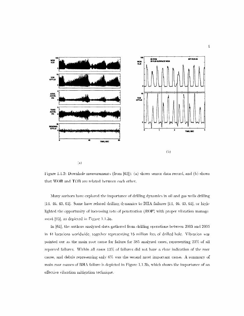
Many authors have explored the importance of drilling dynamics in oil and gas wells drilling

[14, 46, 43, 61]. Some have related drilling dynamics to BHA failures [14, 46, 43, 61], or high-

lighted the opportunity of increasing rate of penetration (ROP) with proper vibration manage-

ment [25], as depicted in Figure 1.1.3a.

In [61], the authors analyzed data gathered from drilling operations between 2003 and 2005

in 44 locations worldwide, together representing 15 million feet of drilled hole. Vibration was

pointed out as the main root cause for failure for 385 analyzed cases, representing 23% of all

reported failures. Within all cases 13% of failures did not have a clear indication of the root

cause, and debris representing only 6% was the second most important cause. A summary of

main root causes of BHA failure is depicted in Figure 1.1.3b, which shows the importance of an

eective vibration mitigation technique.

5

Hence, large vibrations directly impact drilling performance by causing unplanned delays

to replace BHA components or reducing ROP. Therefore, this thesis addresses the challenge of

modeling and analyzing drill string dynamics, in particular the coupled axial-torsional motions,

to support further understanding of the mechanisms involved in the generation of these vibra-

tions. A concise overview of existing work related to the study of stick-slip is given in the next

section.

(a)

(b)

Figure 1.1.3: Vibration importance in oil and gas wellbore drilling: (a) shows schematic perfor-

mance improvement by vibration management (adapted from [25]), and (b) main root causes

leading to BHA failure. Vibration is the most relevant root causes, and debris is the second

identied cause and responsible for only 6% of failures (from [61]).

1.2 Stick-slip Modeling Approaches

Within this sub-section we present the two usual approaches adopted to study drilling dynamics,

and in particular the stick-slip phenomena. First we present what we call the classical approach,

where the study of stick-slip comes from the adoption of a weakening torque-velocity relationship,

which is usually uncoupled from the axial motion. Then we present a model of the self-excited

drill string vibrations, which assumes that the bit/rock interface presents a regenerative eect

that couples axial and torsional motions.

6

1.2.1 Weakening torque-velocity relationship

The classical approach to study the stick-slip phenomena has been to assume a bit/rock interface

law characterized by a weakening torque-velocity response, as for instance in [15, 59, 24]. In [59]

the response is described by a non-linear analytical relationship between frictional torque and

angular velocity Ωo, such as depicted in Figure 1.2.1b. Such a response is akin to the negative

damping observed in drilling jobs. Indeed torque measurements while drilling suggest that the

resisting torque at the bit decreases with increasing Ωo. More specically [15] presents some

results where reduced torque is associated with increasing angular velocity under constant WOB

(Figure 1.2.1a), and points out that it is an inherent PDC bit characteristic. The conclusion

from this study was that stick-slip mitigation is possible by reducing torque through increasing

Ωo or decreasing WOB. However, in [15] there is no explanation for the reasons behind such

torque behavior.

0

0.5

1

1.5

2

2.5

3

0 50 100 150 200 250

Tor

que

(klb

f.ft

)

Ω (RPM)

Sharp PDCDull PDC

Dull PDC in Shale

(a)

-3

-2

-1

0

1

2

3

-60 -40 -20 0 20 40 60

Tor

que

(klb

f.ft

)

Ω (RPM)

(b)

Figure 1.2.1: Torque-friction relationship: (a) Test results from [15], and (b) non linear analytical

approximation from [59],

There are two concerns with the weakening torque-velocity relationship approach. First,

it does not account for the coupling between axial and angular dynamics, even though its

importance is recognized [62]. Second, experiments with kinematic control with single PDC

cutter and tricone bits [27] do not support the weakening torque-velocity relationship. In the

7

latter, the resulting torque is almost constant with increasing Ωo as shown in Figure 1.2.2.

0

5

10

15

20

25

30

0 20 40 60 80 100 120

Tor

que

(N.m

)

Ω/2π (RPM)

Figure 1.2.2: Torque variation with angular velocity for drilling test with a tricone bit and

kinematic control from [27].

1.2.2 Self-excited vibrations

Another approach to model axial and torsional vibrations is to introduce the regenerative eect

into the bit/rock interface law. The regenerative eect has widely been used in models involving

metal cutting to study self-vibrations of machining tools [58, 4, 5, 56]. The insertion of the

regenerative eect to describe the cutting forces results in delay dierential equations (DDE)

[55, 10, 26].

To our knowledge, only a few authors have considered the regenerative eect for self-excited

drilling dynamics. For example [17] studied the uncoupled torsional motion of drilling system

using DDE, but not the axial motion. Interestingly, in [39] the coupled axial and torsional

bit dynamics is numerically evaluated by taking into account the actual forces acting on each

PDC cutter. The coupling between axial and torsional motion was made through the bit/rock

relationship. However, there is no mention about the use of DDE's as a modeling framework.

In [48], the author explored a more comprehensive approach to study the stick-slip problem,

including the regenerative eect, and coupling axial and torsional motions. The lumped model,

8

denoted here as the RGD model [52], is characterized by a set of delay dierential equations [10]

for axial and torsional motion coupled by the bit/rock relationship. Moreover, the authors could

show that the weakening torque-velocity relationship is a consequence of the system behavior,

rather than an intrinsic property of the drilling system as pointed by [15]. After [48], others

authors developed further studies, as for instance [49, 50, 32, 29, 52, 30, 19, 31, 18], and their

works are used as a basis in this thesis. The previous studies were done for the torsional oscillator

with 2-DOF. In [30] a nite element model was used to understand stick-slip conditions in time

domain simulations.

1.3 Objectives

This thesis addresses the study of the stick-slip phenomena using a phenomenological model

based on the regenerative eect. This phenomenological model, imposed as boundary condition

at the bit, couples the axial and torsional motion of the drill string through the variable depth-

of-cut d. A simple angular velocity control system at the surface is compared to a standard

drive system as a stick-slip mitigation solution, even though the control set up is made upon

torque-velocity weakening assumptions.

The role of spatial discretization appeared to be of crucial importance. This issue is addressed

by means of simple models with axial oscillators. Afterwords, the discretization study is extended

to the coupled axial and torsional oscillators, where a hypothetical case of semi-innite drill string

is also studied. The stability study of these discrete system, and their time domain behavior,

are the key to understand stick-slip oscillations, and mitigation possibilities.

1.4 Thesis Structure

This thesis is organized from the continuous system representation to the semi-discretization

problem.

Chapter 2 presents rst a simplied description of a drilling system with relevant information

for the current study. Then the imposed drilling parameters at the surface, and some possible

alternatives to actual rigs are briey introduced. A phenomenological bit/rock interaction law

9

[22] is then presented. This law, in conjunction with a dynamic model of the drilling system,

leads to the formulation of a model described by delay dierential equations. The drill string is

modeled as a continuous wave-propagating medium, on which the imposed boundary conditions

are the drilling parameters at the surface, and the bit/rock interaction law at the bit. The steady-

state problem solution is provided, and dimensionless formulation for the perturbed dynamics

is presented.

The governing equations presented in Chapter 2 are then semi-discretized in Chapter 3,

based on a nite element formulation. The semi-discrete governing equations, representing the

perturbed axial and torsional displacements, are used to understand the evolution of the drilling

dynamics over time, and the conditions leading to stick-slip vibrations. The stability the semi-

discrete form is not assessed, for reasons discussed in the beginning of Chapter 3 and further

explored in Chapter 6.

Chapters 4 and 5 discuss the importance of the spatial discretization used to describe the

dynamics of the drilling system. We start with a simplied model to understand how the

discretization changes the axial drilling dynamics, based on a time scale separation approach

presented in [52]. Lumped models with 2 and 3 oscillators have their stability assessed. The time

behavior based on its stability charts are presented. Time simulation for a 10 axial oscillators

model is presented.

Chapter 6 discusses the main results and limitations of the current study, as well as sugges-

tions for future work.

Chapter 2

Drill String Dynamics Model

This chapter is structured in two main sections. The rst section describes a simplied drilling

system that represents the main features relevant for this study. The second section presents a

general formulation of the drilling system dynamics, with the imposed surface boundary con-

ditions and the bit/rock interface relationship that establishes the boundary conditions at the

bit. Finally, a dimensionless model formulation is presented and the stationary and perturbed

motions are introduced.

2.1 Drilling System Description

The system described here consists of the main components necessary to drill a well: the surface

drive system, the drill string, and the drill-bit. The drive system (rotary table or top drive)

imposes the hook load H and the angular velocity Ω at the surface. The drill string, composed

mainly of drill pipes and drill collars, transmits the vertical force and torque imposed at the

surface to the bit, which drills the rock. The closed-loop circulation drilling uid removes the

cuttings, whose eects are not considered in the present study. Figure 2.1.1a shows a PDC bit

with a view of a PDC cutter, and Figure 2.1.1b illustrates an idealized drill bit of the type

considered in this study.

The coordinate system x is aligned with the borehole, pointing downward. Its origin is at

10

11

the surface. The boundary conditions imposed at the surface, i.e., at x = 0, are the vertical

force (or hook load) H and angular speed Ω.

A bit/rock interface law describes the lower boundary condition (at the bit, i.e., at x = L).

This interface law describes the relationship between the amount of rock removed by the bit

and the applied weight (axial force) and torque on bit (W and T , respectively). The drill-bit is

considered to be rigid and its dimensions can be disregarded in comparison with the total length

of the drill-string (the total length L is the sum of the drill-pipes and BHA lengths, respectively

denoted by Ld and Lb).

The system dynamics is described in terms of the axial and angular displacements (denoted

by U (x, t) and Φ (x, t), respectively), which are measured from a xed reference at the surface.

The drill string eective weight provides the applied weight on bitW . The applied vertical force

H is chosen based on the desired weight on bit W (W =´ L

0A (x) fudx−H, with fu being the

eective weight per unit volume and A (x) the cross sectional area of the drill string) to drill the

well. The axial force F (x, t) and torque T (x, t) elds are the sum of the quasi-static force and

torque (F s and T s) and those arising from the dynamical motion (F d and T d).

It is important to recognize that, although the length of the drill string increases (by adding

more pipes at the surface), the overall dynamics is established during an interval over which the

drill string length is almost constant. In a practical sense, it means that we can evaluate the

entire dynamics of the system for a given wellbore depth or drill string length L.

12

(a)

(b)

Figure 2.1.1: Drill-bit: (a) PDC drill bit with PDC cutter in detail, (b) Idealized drill bit

showing two blades, local frame of reference s − n, depth of cut d (t), worn length `, axial and

angular displacement U (L, t) and Φ (L, t) with respectively delayed displacements U (L, t− t1)

and Φ (L, t− t1) displacements.

2.2 Controllable Parameters and Interface Law

2.2.1 Controllable Parameters

Conventional drive systems attempt to keep the hook load H and drill string angular speed Ω

constant at the surface. If the system exhibits vibration, both H and Ω oscillate due to the

complex nature of the BC at the rig. However, the BC are often simplied to a constant hook

load H (0, t) = Ho and constant angular velocity Ω (0, t) = Ωo, as in [48], for example.

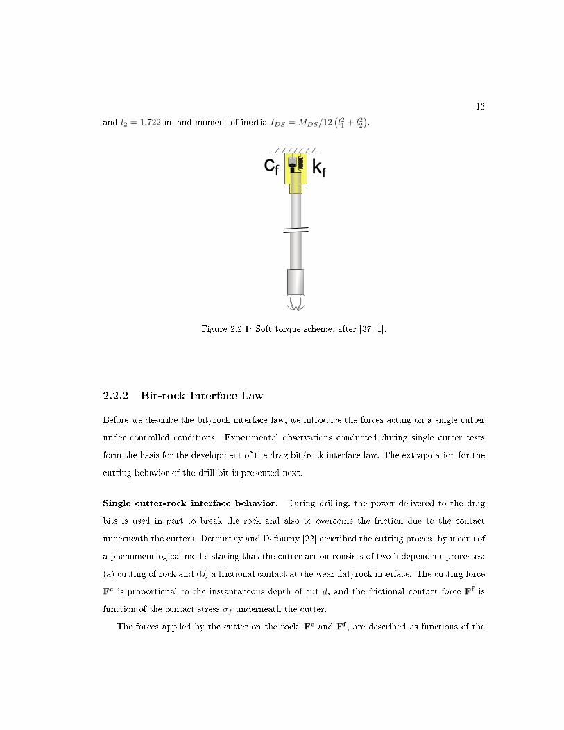
An alternative approach is to consider the presence of the so-called Soft-Torque (ST) [3, 37]

controller in the drive system. ST was designed to be installed in drive systems to mitigate

stick-slip oscillations. The ST system is an angular velocity controller that is represented within

this thesis by a torsional spring and dash-pot at the top boundary condition. The ST system

attempts to damp the dominant (rst) torsional mode for stick-slip. A schematic view of a

drive system with ST is shown in Figure 2.2.1. Herein, the drive system [2] is assumed to be a

rectangular block with mass MDS = 18160 kg, cross-sectional dimensions equal to l1 = 1.867 m

13

and l2 = 1.722 m, and moment of inertia IDS = MDS/12(l21 + l22

).

Figure 2.2.1: Soft torque scheme, after [37, 1].

2.2.2 Bit-rock Interface Law

Before we describe the bit/rock interface law, we introduce the forces acting on a single cutter

under controlled conditions. Experimental observations conducted during single cutter tests

form the basis for the development of the drag bit/rock interface law. The extrapolation for the

cutting behavior of the drill bit is presented next.

Single cutter-rock interface behavior. During drilling, the power delivered to the drag

bits is used in part to break the rock and also to overcome the friction due to the contact

underneath the cutters. Detournay and Defourny [22] described the cutting process by means of

a phenomenological model stating that the cutter action consists of two independent processes:

(a) cutting of rock and (b) a frictional contact at the wear at/rock interface. The cutting force

Fc is proportional to the instantaneous depth of cut d, and the frictional contact force Ff is

function of the contact stress σf underneath the cutter.

The forces applied by the cutter on the rock, Fc and Ff , are described as functions of the

14

intrinsic specic energy (ε), depth-of-cut d, the contact stress (σf ), and the cutter geometry

(cutter width w and blunt length `) [22]:

Fc =

Fcn

Fcs

= εwd

ζ

1

, (2.2.1)

Ff =

Ffn

Ffs

= Ffn

1

µ

. (2.2.2)

The positive sign means that these forces act in the same direction as the cutter velocity,

and the local coordinate system (at the cutter) is dened by the unit vertical axis n pointing

downwards, and the unit horizontal axis s pointing in the same direction as the cutter velocity.

The intrinsic specic energy ε can be understood as the amount of energy necessary to remove

an unit volume of rock, while the parameter ζ characterizes the ratio between the vertical and

horizontal component of force acting on the cutting face. Both ε and ζ can be measured from

single cutter tests.

Now considering that frictional forces are developed under the blunt wear at, the vertical

friction force is a function of contact stress σf and the area of contact (`w). The vertical and

horizontal friction forces can be related through the rate-independent coecient of friction µ:

F fs = µF fn = µσf `w. (2.2.3)

The contact stress assumed is to be constant if the axial velocity V > 0. If there is no

contact, F fs = 0.

Bit-rock interface behavior. The concept developed above for a single cutter can be ex-

tended to a drag bit (see Figure 2.1.1.). The weight W and torque T on bit (now on called

weight- and torque-on-bit, respectively) are comprised by cutting and friction at contact (su-

perscripts f and c ) and forces and torques are written as follows:

W = Wf + Wc, (2.2.4)

T = Tf + Tc. (2.2.5)

The cutting forces are proportional to the depth of cut d and are stated as a function of the

bit radius a, intrinsic specic energy ε, and the depth of cut d, and the number of blades nb.

15

The frictional forces are proportional to the stress underneath the cutters (or blades) σf , and

the contact area. Decomposing the force and torque and assuming that the contact stress σf is

constant throughout the cutters or blades we have the forces acting in the vertical direction:

W c = nbζεad, (2.2.6)

W f = nba`σf . (2.2.7)

The torque will be proportional to the developed forces acting on the bit on horizontal

direction (both cutting and frictional contact).

T c =1

2nbεa

2d, (2.2.8)

T f =1

2nba

2µγ`σf , (2.2.9)

where the constant γ embodies the inuence of the bit design on its mechanical response. If γ

is equal to one it means that the blades are perpendicular to the axis of revolution. The contact

length ` (Figure 2.1.1b) and the bit radius a denes the frictional contact area under the bit.

2.3 Drill String Model

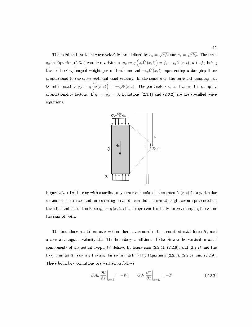
Consider the drill string shown in Figure 2.3.1. The coordinate system x refers to a drill string

cross section position and U (x, t) represents its longitudinal displacement. The axial stress

varies over the element, due to body forces or to accelerations. The quantity qx := q (x, t)

represents the axial body and damping forces per unit volume. The linear momentum balance

for the dierential element with constant cross sectional area A, density ρ, and elastic modulus

E reads:

ρA∂2U

∂t2− EA∂

2U

∂x2+ qx = 0 (2.3.1)

Similarly, the angular momentum balance for constant moment of inertia J , and shear mod-

ulus G reads :

ρJ∂2Φ

∂t2−GJ ∂

2Φ

∂x2+ qφ = 0, (2.3.2)

where Φ (x, t) denotes the angular displacement.

16

The axial and torsional wave velocities are dened by cu =√E/ρ and cφ =

√G/ρ. The term

qx in Equation (2.3.1) can be rewritten as qx := q(x, U (x, t)

)= fu − ςuU (x, t), with fu being

the drill string buoyed weight per unit volume and −ςuU (x, t) representing a damping force

proportional to the cross sectional axial velocity. In the same way, the torsional damping can

be introduced as qφ := q(φ (x, t)

)= −ςφΦ (x, t). The parameters ςu and ςφ are the damping

proportionality factors. If qx = qφ = 0, Equations (2.3.1) and (2.3.2) are the so-called wave

equations.

Figure 2.3.1: Drill string with coordinate system x and axial displacement U (x, t) for a particular

section. The stresses and forces acting on an dierential element of length dx are presented on

the left hand side. The force qx := q (x, U, t) can represent the body forces, damping forces, or

the sum of both.

The boundary conditions at x = 0 are herein assumed to be a constant axial force Ho and

a constant angular velocity Ωo. The boundary conditions at the bit are the vertical or axial

components of the actual weight W dened by Equations (2.2.4), (2.2.6), and (2.2.7) and the

torque on bit T resisting the angular motion dened by Equations (2.2.5), (2.2.8), and (2.2.9).

These boundary conditions are written as follows:

EAb∂U

∂x

∣∣∣∣x=L

= −W, GJb∂Φ

∂x

∣∣∣∣x=L

= −T (2.3.3)

17

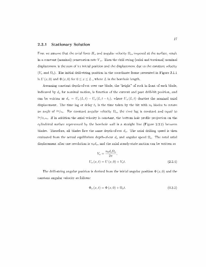
2.3.1 Stationary Solution

First we assume that the axial force Ho and angular velocity Ωo, imposed at the surface, result

in a constant (nominal) penetration rate V o. Then the drill-string (axial and torsional) nominal

displacement is the sum of its initial position and the displacement due to the constant velocity

(Vo and Ωo). The initial drill-string position in the coordinate frame presented in Figure 2.1.1

is U (x, 0) and Φ (x, 0) for 0 ≤ x ≤ L , where L is the borehole length.

Assuming constant depth-of-cut over one blade, the height of rock in front of each blade,

indicated by do for nominal motion, is function of the current and past drill-bit position, and

can be written as do = Uo (L, t) − Uo (L, t− t1), where Uo (L, t) denotes the nominal axial

displacement. The time lag or delay t1 is the time taken by the bit with nb blades to rotate

an angle of 2π/nb. For constant angular velocity Ωo, the time lag is constant and equal to

2π/Ωonb. If in addition the axial velocity is constant, the bottom-hole prole projection on the

cylindrical surface represented by the borehole wall is a straight line (Figure 2.3.2) between

blades. Therefore, all blades face the same depth-of-cut do. The axial drilling speed is then

evaluated from the actual equilibrium depth-of-cut do and angular speed Ωo. The total axial

displacement after one revolution is nbdo, and the axial steady-state motion can be written as

Vo =nbdoΩo

2π,

Uo (x, t) = U (x, 0) + Vot. (2.3.4)

The drill-string angular position is derived from the initial angular position Φ (x, 0) and the

constant angular velocity as follows:

Φo (x, t) = Φ (x, 0) + Ωot. (2.3.5)

18

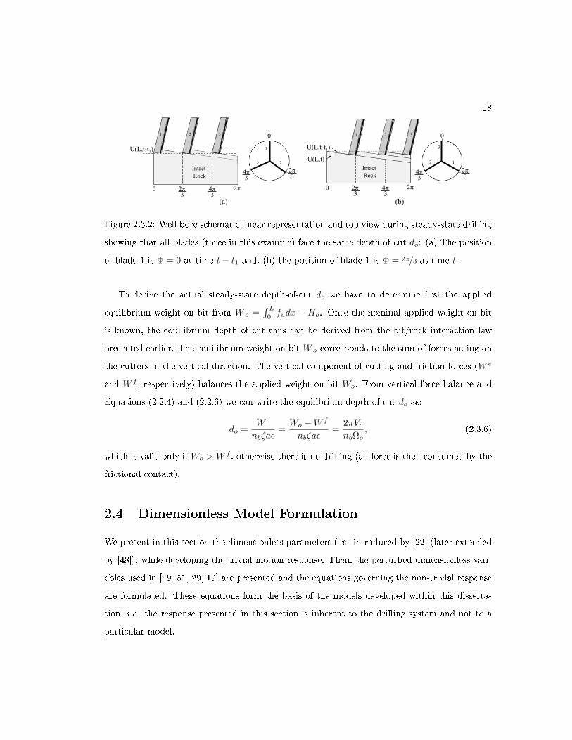
Figure 2.3.2: Well bore schematic linear representation and top view during steady-state drilling

showing that all blades (three in this example) face the same depth-of-cut do: (a) The position

of blade 1 is Φ = 0 at time t− t1 and, (b) the position of blade 1 is Φ = 2π/3 at time t.

To derive the actual steady-state depth-of-cut do we have to determine rst the applied

equilibrium weight on bit from W o =´ L

0fudx − Ho. Once the nominal applied weight on bit

is known, the equilibrium depth of cut thus can be derived from the bit/rock interaction law

presented earlier. The equilibrium weight on bit W o corresponds to the sum of forces acting on

the cutters in the vertical direction. The vertical component of cutting and friction forces (W c

and W f , respectively) balances the applied weight on bit Wo. From vertical force balance and

Equations (2.2.4) and (2.2.6) we can write the equilibrium depth-of-cut do as:

do =W c

nbζaε=Wo −W f

nbζaε=

2πVonbΩo

, (2.3.6)

which is valid only if Wo > W f , otherwise there is no drilling (all force is then consumed by the

frictional contact).

2.4 Dimensionless Model Formulation

We present in this section the dimensionless parameters rst introduced by [22] (later extended

by [48]), while developing the trivial motion response. Then, the perturbed dimensionless vari-

ables used in [49, 51, 29, 19] are presented and the equations governing the non-trivial response

are formulated. These equations form the basis of the models developed within this disserta-

tion, i.e. the response presented in this section is inherent to the drilling system and not to a

particular model.

19

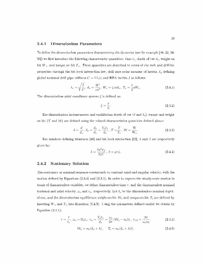
2.4.1 Dimensionless Parameters

To dene the dimensionless parameters characterizing the dynamics (see for example [48, 32, 29,

30]) we rst introduce the following characteristic quantities: time t∗, depth-of-cut d∗, weight on

bit W ∗, and torque on bit T ∗. These quantities are described in terms of the rock and drill-bit

properties through the bit/rock interaction law, drill pipe polar moment of inertia Jp dening

global torsional drill pipe stiness C = GJp/L and BHA inertia I as follows:

t∗ =

√I

C, d∗ =

2C

εa2, W∗ = ζεad∗, T∗ =

1

2aW∗. (2.4.1)

The dimensionless axial coordinate system ξ is dened as:

ξ =x

L. (2.4.2)

The dimensionless instantaneous and equilibrium depth-of-cut (δ and δo), torque and weight

on bit (T and W) are dened using the related characteristics quantities dened above:

δ =d

d∗, δo =

dod∗

=Vot1d∗

, T =T

T∗, W =

W

W∗. (2.4.3)

The numbers dening bluntness [48] and bit/rock interaction [22], λ and β are respectively

given by:

λ =`a2σf2ζC

, β = µγζ. (2.4.4)

2.4.2 Stationary Solution

The stationary or nominal response corresponds to constant axial and angular velocity, with the

motion dened by Equations (2.3.4) and (2.3.5). In order to express the steady-state motion in

terms of dimensionless variables, we dene dimensionless time τ , and the dimensionless nominal

torsional and axial velocity, ωo and υo, respectively. Let δo be the dimensionless nominal depth-

of-cut, and the dimensionless equilibrium weight-on-bit Wo and torque-on-bit To are dened by

inserting W o and T o into Equation (2.4.3). Using the parameters dened earlier we obtain by

Equation (2.4.1):

τ =t

t∗, ωo = Ωot∗, υo =

Vot∗d∗

=ωo2π

(Wo − nbλ) , τ1,0 =2π

ωonb. (2.4.5)

Wo = nb (δo + λ) , To = nb (δo + λβ) . (2.4.6)

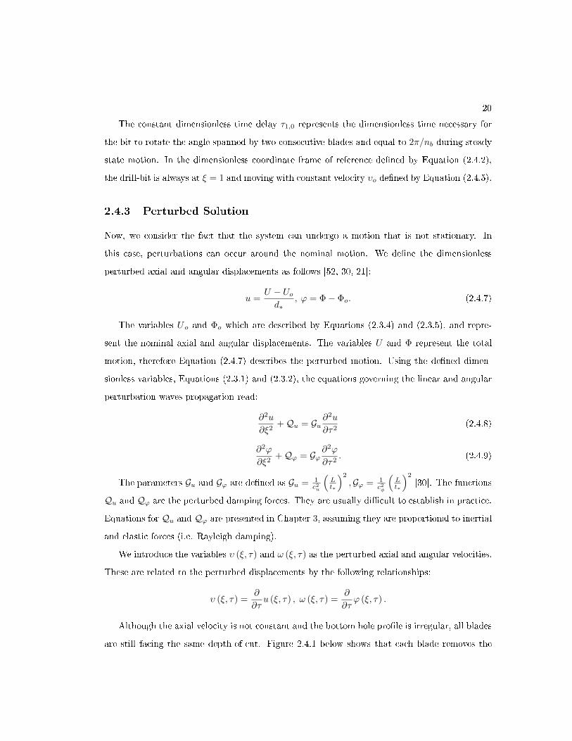
20

The constant dimensionless time delay τ1,0 represents the dimensionless time necessary for

the bit to rotate the angle spanned by two consecutive blades and equal to 2π/nb during steady

state motion. In the dimensionless coordinate frame of reference dened by Equation (2.4.2),

the drill-bit is always at ξ = 1 and moving with constant velocity υo dened by Equation (2.4.5).

2.4.3 Perturbed Solution

Now, we consider the fact that the system can undergo a motion that is not stationary. In

this case, perturbations can occur around the nominal motion. We dene the dimensionless

perturbed axial and angular displacements as follows [52, 30, 21]:

u =U − Uod∗

, ϕ = Φ− Φo. (2.4.7)

The variables Uo and Φo which are described by Equations (2.3.4) and (2.3.5), and repre-

sent the nominal axial and angular displacements. The variables U and Φ represent the total

motion, therefore Equation (2.4.7) describes the perturbed motion. Using the dened dimen-

sionless variables, Equations (2.3.1) and (2.3.2), the equations governing the linear and angular

perturbation waves propagation read:

∂2u

∂ξ2+Qu = Gu

∂2u

∂τ2(2.4.8)

∂2ϕ

∂ξ2+Qϕ = Gϕ

∂2ϕ

∂τ2. (2.4.9)

The parameters Gu and Gϕ are dened as Gu = 1c2u

(Lt∗

)2

,Gϕ = 1c2φ

(Lt∗

)2

[30]. The functions

Qu and Qϕ are the perturbed damping forces. They are usually dicult to establish in practice.

Equations for Qu and Qϕ are presented in Chapter 3, assuming they are proportional to inertial

and elastic forces (i.e. Rayleigh damping).

We introduce the variables υ (ξ, τ) and ω (ξ, τ) as the perturbed axial and angular velocities.

These are related to the perturbed displacements by the following relationships:

υ (ξ, τ) =∂

∂τu (ξ, τ) , ω (ξ, τ) =

∂

∂τϕ (ξ, τ) .

Although the axial velocity is not constant and the bottom hole prole is irregular, all blades

are still facing the same depth-of-cut. Figure 2.4.1 below shows that each blade removes the

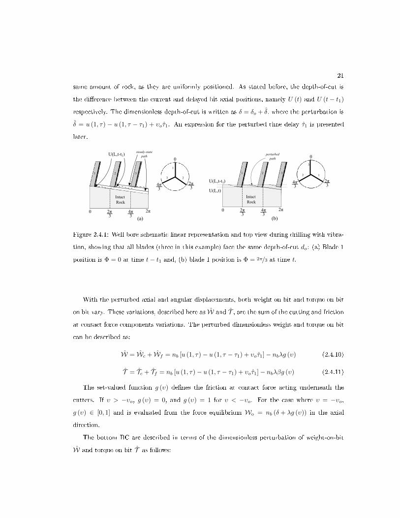
21

same amount of rock, as they are uniformly positioned. As stated before, the depth-of-cut is

the dierence between the current and delayed bit axial positions, namely U (t) and U (t− t1)

respectively. The dimensionless depth-of-cut is written as δ = δo + δ, where the perturbation is

δ = u (1, τ) − u (1, τ − τ1) + υoτ1. An expression for the perturbed time delay τ1 is presented

later.

Figure 2.4.1: Well bore schematic linear representation and top view during drilling with vibra-

tion, showing that all blades (three in this example) face the same depth-of-cut do: (a) Blade 1

position is Φ = 0 at time t− t1 and, (b) blade 1 position is Φ = 2π/3 at time t.

With the perturbed axial and angular displacements, both weight-on-bit and torque-on-bit

on bit vary. These variations, described here as W and T , are the sum of the cutting and friction

at contact force components variations. The perturbed dimensionless weight and torque on bit

can be described as:

W = Wc + Wf = nb [u (1, τ)− u (1, τ − τ1) + υoτ1]− nbλg (υ) (2.4.10)

T = Tc + Tf = nb [u (1, τ)− u (1, τ − τ1) + υoτ1]− nbλβg (υ) (2.4.11)

The set-valued function g (υ) denes the friction at contact force acting underneath the

cutters. If υ > −υo, g (υ) = 0, and g (υ) = 1 for υ < −υo. For the case where υ = −υo,

g (υ) ∈ [0, 1] and is evaluated from the force equilibrium Wo = nb (δ + λg (υ)) in the axial

direction.

The bottom BC are described in terms of the dimensionless perturbation of weight-on-bit

W and torque-on-bit T as follows:

22

∂u

∂ξ

∣∣∣∣ξ=1

= −ψuW,∂ϕ

∂ξ

∣∣∣∣ξ=1

= −ψϕT , (2.4.12)

with ψu = ζεaL/EAb, ψϕ = CL/GJb.

The surface boundaries conditions are assumed to be a constant hook load Ho and a con-

stant angular velocity, Ωo, which corresponds to ∂u/∂ξ = 0 and ϕ = 0, respectively. Another

possibility within this thesis is to assume a constant axial velocity, i.e., impose νo = ∂u/∂τ = 0

instead of ∂u/∂ξ = 0 .

To complete our description, we need to dene the time delay. Once the angular speed is

not constant, the time delay becomes dependent of the state. The state-dependent delay can

be obtained from an implicit algebraic equation, and is equal to the elapsed time for the bit to

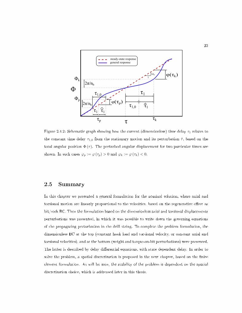
rotate a xed angle 2π/nb. Figure 2.4.2 depicts the total angular bit position Φ as function of the

(dimensionless) time τ . The dashed line represents the steady-state response (Φo = Ωot = ωoτ).

The continuous line represents the response other than the trivial motion. The current di-

mensionless time delay τ1 can be larger or smaller than the constant time delay τ1,0 from the

stationary solution. The implicit algebraic equation dening the current time delay τ1 := τ1 (φ)

is (see [48, 52]):

ϕ (1, τ)− ϕ (1, τ − τ1) + ωoτ1 (1, τ) =2π

nb, (2.4.13)

or in terms of perturbed time delay τ1 (1, τ) = τ1 (1, τ)− 2πωonb

, and reminding that τ1,0 = 2πωonb

is the time delay in the equilibrium conditions (see Equation (2.4.5)):

ϕ (1, τ)− ϕ (1, τ − τ1) + ωoτ1 (1, τ) = 0. (2.4.14)

23

Figure 2.4.2: Schematic graph showing how the current (dimensionless) time delay τ1 relates to

the constant time delay τ1,0 from the stationary motion and its perturbation τ , based on the

total angular position Φ (τ). The perturbed angular displacement for two particular times are

shown. In such cases ϕp := ϕ (τp) > 0 and ϕk := ϕ (τk) < 0.

2.5 Summary

In this chapter we presented a general formulation for the nominal solution, where axial and

torsional motion are linearly proportional to the velocities, based on the regenerative eect as

bit/rock BC. Then the formulation based on the dimensionless axial and torsional displacements

perturbations was presented, in which it was possible to write down the governing equations

of the propagating perturbation in the drill string. To complete the problem formulation, the

dimensionless BC at the top (constant hook load and torsional velocity, or constant axial and

torsional velocities), and at the bottom (weight and torque-on-bit perturbations) were presented.

The latter is described by delay dierential equations, with state dependent delay. In order to

solve the problem, a spatial discretization is proposed in the next chapter, based on the nite

element formulation. As will be seen, the stability of the problem is dependent on the spatial

discretization choice, which is addressed later in this thesis.

Chapter 3

Finite Element Model Formulation

3.1 Introduction

This chapter presents the semi-discrete form of Equations (2.4.8) and (2.4.9), developed based on

a nite element formulation [47, 44]. Stability of the semi-discrete system of equations describing

the drill string dynamics is not analyzed here. There are still unresolved issues in regard to the

role of the discretization on the stability of the system of equations, as rst shown by Liu et al

[40]. These authors studied the stability of a discrete system composed of axial and torsional

oscillators (consisting of a mass and a spring) with dash pots representing the drilling system

with the same bit rock interface law presented here, as depicted in Figure 3.1.1.

The stability study, which was based on the semi-discretization method [34], indicates that

the stable area in the parameter space ωo − υo reduces when increasing the number of degrees

of freedom. The stability result is shown in Figure 3.1.2, with nd and nb being the number

of axial and torsional oscillators representing the DP and BHA, respectively. For instance, a

discrete system with 5 oscillators has a much smaller stability region compared to a system with

only 1 oscillator. For 24 oscillators, there is only a narrow area characterizing stable operating

conditions in terms of νo and ωo.

24

25

Figure 3.1.1: Discrete system representation of drilling system with masses-springs-dash pots

for axial and torsional motions (adapted from [40]).

In Chapters 4 and 5, we study in more detail the eects of the spatial discretization on the

stability of the resulting DDE system of equations. In this current chapter, we only investigate

the occurrence of stick-slip based on time simulations. The benchmark drilling system is the

one already studied in [30]. In doing so, we also study the dynamics of an equivalent system

with ST, which exhibited unstable motion but with slower growth of angular oscillations when

compared to a conventional drive system.

26

Figure 3.1.2: Stable region (high-lighted by shaded area for nd = 20 and nb = 4) in the

dimensionless parameter space ωo − υo with dierent number of degrees of freedom, where nd

and nb are the number of oscillators representing the DP and BHA, respectively (adapted from

[40]).

3.2 Semi-discrete Model Formulation

To solve Equations (2.4.8) and (2.4.9) subject to the boundary conditions at the surface (ξ = 0)

and at the bit (ξ = 1), the governing equations are discretized into n − 1 elements, where n is

the number of nodes. The node labeled as 1 is located at the surface and the one labeled as n

is located at the bit. For more details about the semi-discrete formulation, refer to Appendix

A.1, and also [47, 44, 30]. We can rewrite Equations (2.4.8) and (2.4.9) in semi-discrete form as

follows:

GuMu + χuDu + Ku = F (3.2.1)

GϕJΦ + χϕEΦ+CΦ = T, (3.2.2)

where the matrices and forcing vectors for one element with linear interpolating weighty functions

are given in Appendix A.1, and the assembled matrices M, J, K, and C are given by Equations

(A.1.17)-(A.1.20).

27

Due to the diculty in dening the damping factors χu and χφ, axial and torsional damping

matrices D and E are assumed to be of Rayleigh damping type, i.e. a linear combination of the

mass M (J) and stiness K(C) matrices by the following relationships: χuD = ηuM + ϑuK

and χϕE = ηφJ + ϑφK. The force F and torque T vectors are nonzero at the bit and at the

surface only (the latter depending on the imposed boundary conditions). The reaction force F 1

and torque T 1 at the surface are evaluated for the imposed surface displacement as boundary

conditions. Alternatively, displacements u1 and φ1 at the surface are evaluated for imposed

force and torque boundary conditions at the surface. The applied forces at the bit were derived

in Chapter 2. Equation (2.3.3) denes the bottom BC in terms of total displacements, while

Equation (2.4.12) denes it in terms of dimensionless displacement perturbations.

For both the standard (without any angular velocity controller) and the ST drive system,

the assumed imposed BC is a constant hook load Ho and angular velocity Ωo. But for ST,

it is assumed that internal torque from the drive system (from the equivalent spring-dash pot

system) acts like external torques applied in node 2 (node 1 has prescribed constant torque),

and the drive system mass and inertia (dened in section 2.2.1) are concentrated at node 2.

The external torque acting at node 2, which corresponds to the torque applied by the drive

system is then described by:

GJd∂Φ2

∂x

∣∣∣∣x=x1

= kfΦ2 + cf Φ2, (3.2.3)

which gives the following dimensionless torque perturbation:

∂ϕ2

∂ξ

∣∣∣∣ξ=ξ1

=L

GJd

(kfϕ2 +

cf ϕ2

t∗

). (3.2.4)

Following the proposal in [37], the ST gives optimum performance when its rst natural

torsional frequency is equal to the drill-string rst natural torsional frequency, given that the

drive system damper cf is small. Dening the drive system spring stiness as kf = IDS/t2∗, the

proposed optimum damping ratio in [37] is ξopt ≈√

Γ/2 = 0.06, with Γ = I/IDS . That allows

us to dene the damping parameter as cf = IDS/2ξopt. This design of the ST system in fact

aims do damp the rst torsional resonance mode of the drill-string dynamics.

28

3.3 Time Simulation Results

Time simulations for the benchmark case described by Germay et al [30] were performed to

compare the dierences between a drive system without and with ST. The system has a 1, 000

m long DP, and 200 m long BHA and both cross sectional geometries are described in Appendix

D.1. The spatial discretization has 58 elements (10 representing the BHA), and a forward nite

dierence scheme was used for the time integration. The Newmark time integration method

[6] with the parameters proposed by [8] was also implemented to solve the problem. For the

used small time step size(∆τ = 10−4

), there was no dierence between the results obtained

with these two time integration methods, and we opted for the simple forward Euler method.

Other relevant drilling system properties can be found in Appendix D.1. The axial and torsional

damping factors ϑu and ϑφ were assumed equal to 5.10−4 and 1.10−4, respectively. Both ηu and

ηϕ were assumed to be zero. The drill bit has 6 blades, with nbλ = 5.0, and applied weight on

bit WOB = 15kN . The imposed nominal velocities are νo = 0.47 and ωo = 3.74, and initial

perturbations u, υ, ϕ, ωT = 0.01, 0.01, 0.1, 0.1T were instantaneously imposed to the system

at τ = 0.

The drill bit can present both axial and torsional stick. If axial stick occurs, the axial contact

force is obtained from the force balance by Wf = W −Wc, Wf ≤ nbλ. During axial sticking

the bit can still be rotating.

It is assumed that there is no drilling with angular stick, and axial velocity is also set to zero

in such case. Backward rotation is not allowed, and when the bit presented a (small) negative

angular velocity, it is set to zero. The bit slips when the applied torque on bit overcomes

the reacting bit-rock interface law torque. The torque on bit is evaluated from the system of

equations describing the angular motion.

The time delay τ1 is state-dependent. To solve for the current time delay, it is necessary to

solve the implicit Equation (2.4.14). For the numerical implementation, we search for the angular

bit position equal to the current angular position minus 2π/nb. When looking for the delayed

state u (τp − τ1) and ϕ (τp − τ1), with τp being the time at current time step p, we looked rst

for the position q in the vector of total angular displacement Φ such that Φq ≤ Φp−2π/nb, since

the blades are assumed to be evenly distributed. For the adopted small time step size, linear

29

interpolation was used to nd out τp − τ1, u (τp − τ1) and ϕ (τp − τ1) when Φq 6= Φp − 2π/nb.

A schematic view of the search procedure is shown in Figure 3.3.1. To check the method, the

implicit Equation (2.4.14) must be satised, which means that the residual of its left hand size

must be close to zero.

Figure 3.3.1: Time and state delay search based on total angular displacement vector Φ. First

the position q of Φq ≤ Φp− 2π/nb is determined, relating the position of the delayed states and

making possible to dene time delay. The values to be evaluated are shown inside the box. This

method avoid the need to solve implicit Equation (2.4.14) by numerical methods.

In both cases (without and with ST system), the drill system dynamics showed the three

phases described in [30]: (i) fast axial growth, with axial stick, (ii) increasing angular oscillations,

and (iii) occurrence of stick-slip, as depicted in Figures 3.3.2 and 3.3.3. For the standard

drive system case, it is possible to notice that rst the axial velocity goes to zero, while the

angular velocity oscillates within limited amplitudes, despite the larger applied initial angular

perturbations. After some time, the angular velocity vanishes meaning that the bit enter a

stick phase in both axial and angular motion. As the angular velocity is still applied at ξ = 0,

the torque on bit increases with time, on average linearly, to eventually overcome the reaction

30

torque, causing the system to exit the stick phase. Then, the bit accelerates in the slip phase.

-0.5

0

0.5

1

1.5

2

2.5

3

3.5

4

4.5

0 50 100 150 200 250-10

-8

-6

-4

-2

0

2

4

6

8

10

υ ο +

υ

ωο +

ω

τ

υο + υ

ωο + ω

Figure 3.3.2: Evolution of bit velocities. The dynamics evolves in three phases: (i) axial stick,

(ii) increasing angular oscillations, and (iii) angular stick-slip. Left vertical axis shows axial

velocity, and right one shows angular velocity.

With soft torque, even using the optimum factor proposed by [37], the system still presents

increasing oscillations. It was expected that the ST could minimize, or even mitigate torsional

stick-slip. As evidenced by the simulations results in Figure 3.3.3, fast axial growth still happens.

What is interesting is that there is less upward bit movement compared to the standard drive

system (see 3.3.2). Also the axial amplitude oscillations are smaller. Angular oscillations show

a slower growth rate compared to the previous case. We recall that soft torque only targets

(the damping) of the rst torsional exibility mode and the fact that it has been claimed before

(see for example [60]) that torsional exibility modes at higher frequencies can still trigger stick-

slip oscillations even in the presence of the ST system. Note that, in contrast to the above

publications, which focus on torsional dynamics only and employ a phenomenological velocity-

weakening torque as bit/rock interface law, the results above were obtained for axial-torsional

31

drill string dynamics coupled by the bit/rock interface law introduced in Chapter 2.

The analysis presented above conrms the importance of higher exibility modes for the

modeling and analysis of stick-slip oscillations also in the scope of the type of model presented

in Chapter 2. This observation calls for further research into models for (axial and torsional)

drill-string dynamics including multiple exibility modes and raises the question on what model

complexity is needed to reliably describe such dynamics. The latter is the subject of the inves-

tigation reported in Chapters 4 and 5.

-0.5

0

0.5

1

1.5

2

2.5

3

3.5

4

4.5

0 100 200 300 400 500-10

-8

-6

-4

-2

0

2

4

6

8

10

υ ο +

υ

ωο +

ωτ

υο + υ

ωο + ω

Figure 3.3.3: Bit velocities evolution with ST. The three phases are also presented here. Left

vertical axis shows axial velocity, and right one shows angular velocity.

Figure 3.3.4 shows the low residual obtained by substituting the delayed state and time delay

perturbation in the implicit Equation (2.4.14). Both cases are presented, but for τ ≤ 250 is only

possible to notice the standard drive system case. The overall low residual indicates that the

method provides accurate results.

32

-0.0005-0.00045-0.0004

-0.00035-0.0003

-0.00025-0.0002

-0.00015-0.0001-5ε-005

0 5ε-005 0.0001

0.00015 0.0002

0.00025 0.0003

0.00035 0.0004

0.00045 0.0005

0 100 200 300 400 500

residual w/o EPST

w/ EPST

Figure 3.3.4: Search procedure method check for drill system without ST (τ ≤ 250) and with

ST. The delay state must satisfy Equation (2.4.14), with small residual.

3.4 Discussion

The drilling system described by German et. al. [30] was chosen as benchmark case to study

ways to manage and mitigate stick-slip. But, during our literature review, we faced the spatial

discretization problem, which is that the spatial discretization choice has direct impact on the

system stability. For this reason, the stability of the semi-discrete system of equations based

on nite element formulation was not studied. Hence, vibration mitigation by the choice of the

imposed axial and angular velocities was not possible.

Another option to manage vibrations was to consider a drive system with angular velocity

control, or Soft-Torque. The ST control was implemented as an actual spring and damper ele-

ments connecting the drive system to the upper drill string end, according to [37]. Both time

domain simulations presented the same pattern, with fast development of axial oscillations,

33

resulting in axial stick. The angular velocity oscillations grow slowly compared to axial oscilla-

tions. In particular, the ST delayed the angular oscillations growth compared to the standard

drive system. But, the ST case presented backward rotation, and then the simulation stopped.

Regarding to the numerical time integration scheme, we tested simple Forward Euler and

Newmark's method. For the small step size used, they did not present dierences in the results.

But for the Newmark's method, the integration parameters proposed by [8] introduces a (slight)

numerical damping into the scheme. For that reason, we kept the Forward Euler as the numerical

integration scheme.

A numerical integration based on event driven and variable time step size [9, 54, 16] should

be implemented, especially because of the occurrence of stick phases. The current scheme sets

the angular velocity equals to zero when it is suciently close to it. But with the xed time

step, the axial state correction is compromised. Also the event driven scheme will be very useful

to look for backward rotation and bit bounce.

In order to solve for the state dependent delay, instead of solving the implicit non-linear

Equation (2.4.14), we looked for the time delay based on the drill-bit angular position. It corre-

sponds to the time taken for the bit to rotate the (constant) angle spanned by two consecutive

blades. The evaluated time delay and angular delayed state obeyed Equation (2.4.14) with low

residual, showing that the scheme worked as expected.

Chapter 4

Axial Dynamics of Discrete Drilling

Models

In this chapter, we address the following question: how does the choice of the drill string spatial

discretization impacts its stability? This question arises from the observations of [40], that

were briey presented at the beginning of Chapter 3. To understand the impact of the spatial

discretization, rst we present the stability of axial motion based on time scale separation (see

for example [26]) of the RGD model [29], which allow us to study a simplied partially uncoupled

axial and torsional system. The well-known stability for a lumped axial one DOF system is rst

introduced. Then the stability and time behavior of discrete systems representing the axial

dynamics of the drill string is presented, on the basis of a 2 and 3 DOF representation. The

behavior of a multi-DOF system is also analyzed. For 2 and 3 DOF, the stability analysis

is assessed using semi-analytical tools. For larger order models, stability is conducted with

numerical tools, as the use of analytical tools in such case becomes too complicated. Time

simulation results for all these models display an interesting phase locking behavior.

The analysis of lumped MDOF models is also interesting from another perspective. Namely,

Chapter 3 has revealed that higher exibility modes are important to describe the instabilities

leading to stick-slip oscillations. This raises the question of how the representation of the system

with additional DOF (introducing additional exibility modes) aects such instabilities. This

34

35

question is interesting in its own right, but also bears relevance in the scope of constructing

models serving as a basis for the future development of controllers outperforming ST, although

the latter is outside the scope of this thesis.

4.1 RGD Model

The drill-string in the RGD model is represented by a torsional pendulum for the angular motion

and a dead load on a cable for the axial motion (see Figure 4.1.1a), which is excited by the bit-

rock interaction law introduced in Section 2.2.2. This model exhibits self-excited vibrations

caused by the regenerative eect (and is formulated in terms of delayed dierential equations or

DDE's). The axial and torsional equations of motion are given by:

∂2u

∂τ2= −ψnb [u (1, τ)− u (1, τ − τ1) + υoτ1]− nbλg (υ) , (4.1.1)

∂2ϕ

∂τ2+ ϕ = −nb [u (1, τ)− u (1, τ − τ1) + υoτ1]− nbλβg (υ) . (4.1.2)

If we think of the drill-bit physics, oscillations in the axial direction will lead to oscillations in

depth-of-cut d (see Figure 2.4.1). Oscillations in d result in oscillations of forceW c and torque T c

(see Equations (2.2.6) and (2.2.8)). Also axial oscillations can result in loss of contact underneath

the cutters if the drill bit is moving upward, introducing an additional and important variation

in force Wf and torque Tf (see Equations (2.2.7) and (2.2.9)). It means that the self-excitation

at the bottom-end of the drill-string is oscillatory.

The results from [52] shown in Figure 4.1.1b suggest that axial oscillations trigger angular

oscillations as conrmed by a stability analysis [52, 31]. The study of axial motion as an

independent system comes from the recognition that the RGD model presents a clear time scale

separation between axial and torsional dynamics if the system number ψ is large, as is usually

the case. Figure 4.1.1b illustrates the RGD model response for a typical drilling system [52].

The dimensionless quantities describing the problem are νo = 1.74, ωo = 5, λ = 5, β = 0.3.

The axial motion presents a much smaller period (time scale) than the torsional one. Also in

the early time the axial dynamics is well established while the torsional mode has no signicant

variation. Therefore understanding the axial dynamics is helpful to understand the overall

system behavior.

36

(a) RGD model.

0

1

2

3

4

5

6

0 0.5 1 1.5 2 2.5 3 3.5 4

velocity

τ

ωο+ω

υο+υ

(b) Time scale separation.

Figure 4.1.1: RGD model: (a) system representation, and (b) time evolution with time scale

separation forWo = 7, λ = 5, ωo = 5, ψ = 50, β = 0.3, nb = 6, after [52]. Axial motion presents

higher frequency compared to torsional one (bottom left), while around the equilibrium point

the bit angular speed ω is nearly a constant for a few axial oscillations (bottom right). The

axial motion stability can be assessed based on critical angular speed ωc.

37

In view of the time scale separation, there is an initial short time when the axial vibrations

develop under almost constant angular velocity. Under these conditions we can decouple Equa-

tions (4.1.1) and (4.1.2) assuming that within this interval the time delay (i.e. the torsional

velocity) is almost constant. Then, for the axial motion, the system is (marginally) stable for

an applied angular speed ωo larger than the critical angular speed ωco =√

8ψ/nb. Otherwise,

the system is unstable [52].

The stability of coupled axial and torsional RGD model was further investigated by [20],

following the linearization procedure from [36]. Basically the authors concluded that the linear

system describing the RGD model always presents unstable motion. On the one hand, if the

imposed angular speed ωo is larger than a critical angular speed ωc, the system is in a slow

regime of instability that is associated with the torsional dynamics. On the other hand, if ωo is

smaller than a critical angular speed ωc, the system is dominated by the axial dynamics in the

so-called fast regime, which is characterized by a fast growth of the oscillations compared to the

torsional mode. The critical speed ωc calculated in [19] was close to the one with constant time

delay ωco obtained in [52, 31].

The stability of some classes of second-order autonomous DDE with constant delay was

studied by [12, 33], who analytically developed stability charts for DDE based on Pontrjagin

conditions [45].

The stability chart for systems described by DDE of the type

u (τ) + pu (τ) + au (τ)− bu (τ − 1) = 0

is shown in Figure 4.1.2, noting that the scaling of time is such that the time delay is 1. RGD

model axial dynamics is dened by Equation (4.1.1), and has the same form of the DDE presented

above with a = b = ψ (2π/ωonb)2and p = 0. Based on the stability chart depicted in Figure

4.1.2, the RGD axial dynamics is marginally stable for ψ ≤ 0.25 (ωonb)2or unstable for all other

values of ψ (noting that ψ > 0).

38

Figure 4.1.2: Stability chart for systems with constant delay τ1 = 1 and governing equation of

type u (τ)+pu (τ)+au (τ)−bu (τ − τ1) = 0. Inside the curves, the shaded area represents stable

region for p = 0 , and for p > 0 the stable region is within curves (adapted from [12, 33]). Close

view on the right, making possible to dene RGD model instability boundary.

According to the stability chart shown in Figure 4.1.2, the system is asymptotically stable

if the parameters fall within the shaded area. A lumped model with a > b describes a system

with an axial spring linking the mass to the top boundary condition [11, 42]. Hence, the axial

dynamics can be stable if the axial displacement is imposed at the surface, instead of a force.

For such a case, the axial equation of motion is written as u (τ)+(ψ + κd)u (τ)−ψu (τ − τ1) = 0

for constant angular velocity and κd > 0 represents the presence of the spring. In particular, if

kd < 0 (or a < b), the spring presents a negative stiness, which is not physically relevant. We

also can see that an introduction of a damping-like term into the second order DDE enlarges

the stable area (the curves for which p 6= 0).

39

4.2 Axial Motion of a 2 DOF System

4.2.1 Equations of Motion

In the previous section, we described how the axial dynamics triggers the system instability in

the RGD model. The stability and time evolution for a 2 axial DOF model is now studied.

This model, depicted in Figure (4.2.1a), represents a system with constant angular velocity Ωo

imposed at the surface and with masses M1 and M2 rotating at the same uniform velocity Ωo.

The total system mass and stiness was kept constant, i.e. the 2 DOF discrete model is just

another representation of the same drilling system already presented in the previous section.

The equations of motion are described in terms of the parameters a and b to make it possible

to compare this model with the 1 DOF model. The mass, whose position is given by U2 (t) is

excited by the force from the bit/rock interface for a sharp bit (no friction force component).

The parameter ε describes the relation between the two masses and the system total mass M ,

i.e., M1 = εM , and M2 = (1− ε)M . Also ε relates the two spring stiness to the overall

stiness k as k1 = k/ε and k2 = k/ (1− ε). To conserve the system total mass and stiness, ε is

dened as ε ∈ (0, 1).The governing equations are written in the following form: u1 (t)

u2 (t)

+ K

u1 (t)

u2 (t)

+ B

u1 (t− 1)

u2 (t− 1)

=

0

0

(4.2.1)

K =

( 11−ε + 1

ε

)κdε − κd

(1−ε)ε

− κd(1−ε)2

(1

1−ε

)(κd

1−ε + nbψ) , B = −

0 0

0 nbψ1−ε

. (4.2.2)

In the above equations, κd = t2∗EAd/ (LDPM) represents the squared ratio of two time

scales, i.e., one corresponding to t∗ and the other to the rst natural axial period of oscillations

of the drill-pipes. For ε → 0 or ε → 1, we have M1 → 0 or M2 → 0 and k1 →∝ or k2 →∝,

and we thus recover the 1-DOF model with a spring connecting the mass to the top prescribed

boundary condition. To recover the original parameters from [12] we dene ε → 0 or ε → 1,

κd + κr = a, and κr = nbψ = b .

40

(a) 2-DOF axial model. (b) 3-DOF axial model.

Figure 4.2.1: Multi DOF axial model: (a) Two axial oscillators model; (b) Three axial oscillators

model.

4.2.2 Stability Analysis

The stability analysis has been performed based on Pontrjagin conditions [45], which is pre-

sented in more details in Appendix C.1. The D-subdivision method [34], giving the D-Curves,

and a numerical method to nd out the right-most eigenvalues of the characteristic polynomial-

exponential [63] were also used when it was not possible to nd the parameters satisfying Pon-

trjagin conditions for stability.

The D-Curves are a set of curves in the parameter space associated with a particular imag-

inary conjugate pair of characteristic exponents in the form z = iy, where y is the angular

41

frequency of oscillation. Inside a region bounded by two adjacent D-Curves the system is char-

acterized by the same number of unstable exponents (the D-Curves correspond to a particular

combinations of parameters for which the exponents cross the imaginary axes of the complex

plane). Knowledge of the number of unstable exponents for one particular point inside a region

limited by D-Curves in the parameter space is sucient to dene the system stability inside

that region.

Pontrjagin conditions represent stability criteria for the characteristic exponential polynomial

H (z), z ∈ C, that describes a delayed system. Assuming that z = iy, y ∈ R, the characteristic

exponential polynomial can be rewritten as H (iy) = F (y) + iG (y). If H (iy) has a principal

(see Appendix C.1) term, then all the roots of H (iy) have a negative real part if the following

conditions are satised:

1. All zeros of F (y) (or G (y)) are real, and;

2. For every zero of F (y) (or G (y)) , F ′ (y)G (y) < 0 (or F (y)G′ (y) > 0) holds.

For the characteristic polynomial pertaining to Equation (4.2.1), it is not dicult to show that all

zeros of G (y) are real. Then we have to look for which values of (a, b) condition 2 above holds to

dene the system stability. The stability analysis is then presented in the same parametric space

(a, b) used to describe the single axial oscillator case, presented in Figure 4.1.2. We can dene a

as the term multiplying the current axial state u (τ), and b as the one multiplied by the delayed

stated u (τ − τ1). The stability charts in the original parameter space (a, b) are shown below,

for some values of ε. The triangle in black shows the stability boundaries, already presented in

Figure 4.1.2, which allow us to compare the 2-DOF and 1-DOF approximations. The curves in

both pictures represent loci where there are two imaginary eigenvalues, i.e. z = ±iy, except for

the line a = b representing the locus where z is identically equal to zero.

We can see that for small values of ε the stability boundary is almost the same for the 1-DOF

model. In fact, a small ε means that our system representation is really close to the 1-DOF one,

with a really rigid upper spring connecting the imposed top boundary condition to a small mass.

The lower mass M2 and the lower spring k2, which accounts for almost all system mass and

compliance, are directly subjected to the excitation provided by the bit/rock interaction.

When ε increases, the stability sub-region near the origin of the parametric space becomes

42

itself disconnected. A narrow stability band exists close to the line a = b. This comes from

the fact that the locus z = ±iπ (see Figure 4.2.2) dened by the projection of a hyperbolic

paraboloid on plane (a, b), goes apart with increasing ε.

Let us consider two similar representations, with ε = 0.2 and ε = 0.8, respectively. In both

cases, the eigenvalue problem without the time delay term is the same. But the stability regions

showed in Figure 4.2.2 changes drastically. This result suggests that the response is not only a

function of the discrete system eigenmodes (otherwise the stability for these two cases should

be the same). The delay introduced by the bit/rock relationship evidently plays a key role in

the overall system stability.

Figure 4.2.2: Stability charts for 2-DOF system in a − b parameter space dened by

Equation(4.2.1) with ε = 0.005, 0.2, 0.5 on the left and ε = 0.2, 0.8 on the right. On the

left, darkest shadow represents stability for ε = 0.5, while on the right, it represents stability

for ε = 0.8. The curves represent loci characterized by a pair of purely imaginary eigenvalues,

exception for the line a = b, where the both real and imaginary parts are identically null (note:

only selected curves are presented for the sake clarity).

The system with identical masses and springs (ε = 0.5) was further studied, because it is

the basis of the representation of the drilling system, with equal masses and springs. First we

43

extended the space parameter region, where we studied the stability. Figure 4.2.3a shows three

disconnected areas representing stable regions for the axial system. Figure 4.2.3b shows a closer

look of the parameter space and a more detailed stability chart. This gure shows two paths

dened by lines L1 and L2 along which the evolution of the right-most eigenvalues was studied.

It also shows the so-called D-Curves, which are labeled with the value of the corresponding

imaginary eigenvalue pair. The only exception is for the line where a = b, in which there is

only one eigenvalue crossing the imaginary axis. In this particular case, both real and imaginary

parts are zero. This particular eigenvalue is here denoted as zo.

To understand how the right-most eigenvalues evolve with the system parameters a and b,

these two parameters were varied according to the paths dened by L1 and L2. Usually, at most

one pair of eigenvalues crosses the imaginary axis within both L1 and L2. This eigenvalue pair

is herein denoted z1 and z1. Cases A1 and A2, depicted in Figure 4.2.3b, show where another

eigenvalue pair, referred to as z2 and z2, crosses the imaginary axis instead of z1 and z1. A third

eigenvalue pair was also found. This pair is always stable and its path is no longer studied.

(a) Stability of two DOF model.(b) Stability of two DOF model for ex-

tended parameter space.

Figure 4.2.3: Stability chart for 2-DOF of system with equal masses and springs: (a) stable

regions dened by shaded areas, and (b) paths L1 and L2 over which the most-right eigenvalues

evolution were studied. The values over the lines show =(z) for which <(z) = 0. Most right

eigenvalues for A1 and A2 are showed in detail in Figure 4.2.4.

44

The overall eigenvalues evolution along L1 and L2 is shown in Figure 4.2.4. The arrows shows

the eigenvalues evolution for (a, b) moving from right to left. Cases A1 and A2 are depicted by

diamonds. For unstable eigenvalues, the path is red. For stable, it is blue. The light green color

means that the exponent z2 is located on the imaginary axis, i.e., < (z2) = 0. The detailed view

in Figure 4.2.4a shows the location of eigenvalues z1 and z2 for case A2, and in Figure 4.2.4b

shows z2 when (a, b) is at the right end of L2. Pair (z1, z1) crosses the imaginary axis six times

at ±qπ, q = 1, .., 7, while (z2, z2) crosses only at ±π and ±2π.

Location of pairs (z1, z1) and (z2, z2) denes the stability of the system. If both are in the

left-hand side of the complex plane, i.e. < (zp) < 0, p = 1, 2, the system is dened as stable. The

pair z1 and z1 crosses most often the imaginary axis. Only at points A1 and A2 in Figure 4.2.3b,

the crossing takes place for pair (z2, z2). If we are moving over paths L1 and L2 from right to

left end, the pair (z2, z2) is stable until we reach point A1. The rst eigenvalues crossing is z1

at ±7π, and the next crossing occurs when z1 is at ±6π. Between these two crossings, (z1, z1)

are stable, which means that the system is stable (remembering that z2 and its conjugate are

stable and did not cross the imaginary axis yet).

The next crossing point is dened by A1, with z2 ,z2 crossing at ±2π. From now on, the

system is unstable until we reach A2. The pair z1,z1 crosses at ±5π, ±4π, and ±3π. At A2,

z2 crosses to the left side of the complex plane at ±π, and from now on z2 and z2 are always

stable. Also at point A2, pair z1,z1 is stable, so does the system. The last two (z1, z1) crossing

are at ±2π (becoming unstable) and ±π (becoming stable), respectively.

At a = b , (z1, z1) and (z2, z2) collapse to a single eigenvalue located at the real axis. Since

zo is always located over the real axis, in a = b we have three eigenvalues over the real axis, and

one of them is located at the origin. This condition is represented by the triangles of Figure

4.2.4.

45

(a) Right-most eigenvalues for path L1.

(b) Right-most eigenvalues for path L2.

Figure 4.2.4: Right-most eigenvalues evolution for (a, b) changing over lines L1 and L2 from

right to left end. Diamonds represent positions of eigenvalues z1 and z2 at cases A1 and A2.

Triangles represent the eigenvalues positions for a = b. Red and blue path represent instability

and stability respectively. The diamonds represent locations at which < (z2) = 0. (a) detail

shows location of z1 and z2 for case A2 in L1; (b) detail shows z2 location for (a, b) = (50; 0.3)

in L2.

46

4.2.3 Time-Domain Simulations

Time-domain simulations were performed in reference to the stability diagrams presented above,

and the solutions agreed with the stability conditions, as can be seen in Figures 4.2.5. Three

dierent cases were studied in time-domain. Among then, only one case is located in a stable

area in the stability chart (Figure 4.2.5e), while the other two are located in the unstable

regions (Figures 4.2.5a and 4.2.5c). Interestingly the system presents phase locking, i.e., the

oscillators are vibrating at the same common frequency, with or without phase shift [53, 57].

For systems represented in the parametric space farthest from the origin, the oscillator are in

phase, i.e.,|φi − φj | ≈ 0. However, for parameter values closer to the origin, the oscillators

present a phase shift, i.e., |φi − φj | ≈ π. Figure 4.2.5 shows the results for two dierent points

in the parameter space. Figure 4.2.5a illustrates the response for a system represented by

(a, b) = (6.9, 2.96). It is an unstable system according to Figure 4.2.2, and the oscillations grow

exponentially. But the two oscillators are in phase. Figure 4.2.5e shows the time response for a

system with (a, b) = (0.35, 0.3), which is stable according Figure 4.2.2. Indeed the time response

is asymptotically stable, but the masses are vibrating with a π-phase shift before vanishing.

For the case (a, b) = (3.45, 2.96) the system is unstable and the oscillators are out-of-phase (see

Figures 4.2.5c and 4.2.5d).

47

-0.004

-0.003

-0.002

-0.001

0

0.001

0.002

0.003

0.004

0 20 40 60 80 100

u

τ

(a) Two-oscillator model in phase.

-0.001

-0.0005

0

0.0005

0.001

46 48 50 52 54

u

τ

top

bottom

(b) Two-oscillator model in phase detail.

-0.0004

-0.0003

-0.0002

-0.0001

0

0.0001

0.0002

0.0003

0.0004

0 20 40 60 80 100

u

τ

(c) Two-oscillator model out-of-phase.

-0.0002

-0.00015

-0.0001

-5ε-005

0

5ε-005

0.0001

0.00015

0.0002

50 51 52 53 54 55 56 57 58

u

τ

top

bottom

(d) Two-oscillator model out-of-phase. detail.

-0.0004

-0.0002

0

0.0002

0.0004

0.0006

0.0008

0.001

0.0012

0 10 20 30 40 50 60

u

τ

top

bottom

(e) Stable two-oscillator model.

Figure 4.2.5: Time response for 2-oscillator model systems located at: (a) and (b) (a, b) =

(6.9, 2.96), (c) and (d) (a, b) = (3.45, 2.96), and (e) (a, b) = (0.35; 0.3).

To understand the phase rule between the oscillators, we dene the eigenvalues as z = x+ iy,

x, y ∈ R and describe the solutions by:

u1 = U1ezt+iφ1

u2 = U2ezt+iφ2 .

48

Substituting the above equations into Equation (4.2.1) we obtain the following non-linear system

of equations:

x2 − y2 + 4α(2− r cosφ) = 0

xy − 2αr sinφ = 0

x2 − y2 + 4α(1− r−1 cosφ) + 2b(1− e−x cosx) = 0

2xy + 4αr−1 sinφ+ 2be−x sinx = 0,

with r = U1/U2 and φ = φ1 − φ2. For L1 and L2, we know the right-most eigenvalues values

(x, y). Solving the above system for φ yields:

cotφ =x2 − y2 + 8α

2xy

From Figures 4.2.4a and 4.2.4b we note that x is O(10−1

)and y is O

(101)at the right

ends of L1 and L2. It means that φ→ 0 or φ→ π. Specially when z1 is the dominant mode, x

is O(10−2 − 10−3

), α and y are O

(100)and O

(101), respectively. When z2 presents real and

imaginary parts of the same order of magnitude, both z1 and z2 are stable. Then the imaginary

part of z1 is O(100). Hence, the masses can oscillate only in or out-of-phase.

4.3 Axial Motion of 3-DOF System

The perturbed equations of motion were derived so as to keep the overall mass and stiness

constant, as done before. Parameter ε establishes the relation between total and individual

masses and stinesses. The equation of motion can be written as:u1 (t)

u2 (t)

u3 (t)

+ K

u1 (t)

u2 (t)

u3 (t)

+ B

u1 (t− 1)

u2 (t− 1)

u3 (t− 1)

=

0

0

0

(4.3.1)

K =

2κdε2 −κdε2 0

−κdε22κdε2 − κd

(1−2ε)ε

0 − κd(1−2ε)2

11−2ε

(κd

1−2ε + nbψ) , B =

0 0 0

0 0 0

0 0 nbψ1−2ε

.

49

In this case it, is not easy to apply the Pontrjagin conditions for the stability analysis.

Hence, the D-Subdivision method was applied to determine the conditions for which a conjugate

eigenvalue pair crosses the imaginary axis. Then, using a numerical MatLab package [63], we

search for the number of unstable exponents inside each region dened by the D-Curves. The

resulting stability chart is depicted in Figure 4.3.1 below. For comparison, the case with only

one mass is presented by the black line.

We note again that for small value of ε the system behaves almost like the 1-DOF presented

earlier (but the stable area is reduced compared to the 2-DOF case). When the three oscillators

are identical, the stable region reduces even more when compared to the 2-DOF case, leaving a

narrow stable area.

Figure 4.3.1: Stability chart for 3-DOF system with two dierent congurations.

Time simulations for 3-DOF also show phase locking. If the system parameters are close

to the line a = π2 − b, which is the right boundary of the stable region for ε → 0 in Figure

4.3.1, all oscillators are in phase. If the system is located more on the left side, close to the line

a = b, the oscillators are out-of-phase. During transient motion, the motions of the oscillators

50

are delayed compared to each other. It means that a compressional wave is propagating through

them. After that, the oscillations follow eventually an in or out-of-phase pattern.

-4

-2

0

2

4

0 10 20 30 40 50

u

τ

-4

-2

0

2

4

47.5 48 48.5 49 49.5 50

u

τ

top

middlebottom

(a)

-20

-10

0

10

20

0 10 20 30 40 50

u

τ

-30

-20

-10

0

10

20

30

47.5 48 48.5 49 49.5 50

u

τ

bottom

middle

top

(b)

Figure 4.3.2: Time response for 3-DOF system located at: (a) (a, b) = (6.9, 2.96), (b) (a, b) =

(3.45, 2.96).

4.4 Axial Motion of Multi-DOF System

Suppose that we have a system with N oscillators. The individual masses are M i = ε1M

for i = 1, 2, .., N − 1, and the bottom mass MN = (1− (N − 1) ε1)M , conserving the system

total mass. The same is done for the spring stiness connecting the masses, ki = EAd/ (Ldε2)

for i = 1, 2, .., N − 1 and the bottom spring is kN = EAd/ (1− (N − 1) ε2)Ld. The system

of equations of motion is written in terms of the dimensionless perturbed displacements ui,

51

i = 1, 2, .., N as:

u1

u2

...

uN−1

uN

+ K

u1

u2

...

uN−1

uN

−B

u1

u2

...

uN−1

uN

=

0

0

...

0

0

, (4.4.1)

with the non-zeros entries for matrices K and B written as:

K =

2κdε1ε2

−κdε1ε2

0 ... 0

−κdε1ε2

2κdε1ε2

−κdε1ε2

... 0

... ... ... ... ...

κdε1

[1ε2

+ 11−(N−1)ε2

]−κd

ε1−(N−1)ε1ε2

−κd/[1−(N−1)ε1][1−(N−1)ε2]

11−(N−1)ε1

(κd

1−(N−1)ε2+ nbψ

)

B =

0 0 0 ... 0

0 0 0 ... 0

0 0 0 ... 0

... ... ... ... ...

0 0 0 ... nbψ1−(N−1)ε1

.

The semi-analytical stability analysis is not presented here for N ≥ 4, due to its complexity

and also because a stability analysis of a system of three identical oscillators shows that there is

almost no stable area. The dynamics for a system with 10 identical oscillators (ε1 = ε2 = 0.1) also

presents a synchronous pattern, as shown in Figure 4.4.1. For some systems, all the oscillators

are in-phase (Figure 4.4.1a). But for other systems (as in Figure 4.4.1b), there exists two groups

of oscillators, a lower and upper one which are internally in phase, but the two groups are out-of-

phase. In both cases, the transient vibrations reect the propagation of a wave. The excitation

from the bit/rock interface propagates up and down through the oscillators, which eventually

become synchronized.

52

-20

-15

-10

-5

0

5

10

15

20

0 10 20 30 40 50

u

τ

-20

-15

-10

-5

0

5

10

15

20

47.5 48 48.5 49 49.5 50

u

τ

123456789

10

(a)

-30

-20

-10

0

10

20

30

0 10 20 30 40 50

u

τ

-30

-20

-10

0

10

20

30

40

47.5 48 48.5 49 49.5 50

u

τ

123456789

10

(b)

Figure 4.4.1: Masses displacement time evolution for 10-DOF system located at: (a) (a, b) =

(6.9, 2.96), (b) (a, b) = (3.45, 2.96). In the rst case, all masses are closely in-phase, while in

the second case are two dierent clusters moving out-of-phase, with masses within each cluster

moving in-phase. Masses M1 to M5 composes one in-phase cluster, while the others composes

other cluster.

4.5 Discussion

In this chapter, we studied how the spatial discretization of a given drilling system aects the

overall dynamical behavior. Based on the time scale separation between the axial and torsional

dynamics, the axial dynamics of the drilling system with a sharp bit was uncoupled from the

angular dynamics, and hence studied separately. The semi-analytic stability study of the drilling

system showed that the system axial stability changes within the same parameter space, when

53

rening its discrete spatial representation. For instance, for two equivalent 2-DOF systems,

where the masses, springs, and eigenfrequencies were the same, but with elements swapping

position in relations to the BC's, the stability analysis showed a considerable change in the

stable area. Moreover, increasing the number of DOF's, for instance from 2 to 3, resulted in

a more unstable system. Although the Pontrjagin's conditions make it possible to study the

stability of a characteristic exponential-polynomial of any order, the complexity faced to study

the axial system with 3-DOF did not encourage us to perform the same analytic study to assess

system stability with larger number of DOF's.

For a system represented by a 2-DOF model with equal masses and springs, the evolution of

the right-most eigenvalues when varying linearly the system parameters was studied. This study

showed the possibility of phase locking between oscillators, i.e. the phase dierence between

oscillators remains constant over time during the steady-state response. Even more interesting,

the studied showed that the oscillators are able to be approximately in- or 180oout-of-phase.

The time simulation of the drill string axial motion showed that phase-lock pattern, also for

a larger number of DOF's. For cases with 3 and 10 DOF's, two interesting motion patterns

occurred. In the rst one, all masses were in phase. In the second pattern, the drill string

top and bottom were in out-of-phase motion. We can make a parallel between the 3-DOF and

10-DOF models response. For the 10 DOF model, the top masses cluster presented an in-phase

motion, as well as the bottom masses cluster. But these two cluster were in an out-of-phase

motion compared to each other. Compared to the 3-DOF model representation, it means that

the top cluster in the 10-DOF model is represented by the top mass in the 3-DOF model. The

same occurred for the bottom cluster, represented by the bottom mass in the 3-DOF model.

But in both cases, there was a mass located at the center (mass 2 in the 3-DOF, and mass 6 in

the 10-DOF models) with minimum displacement compared to the others.

Now, we have to look if the stability of a coupled system is also aected by the spatial

discretization, and if there is any phase locking pattern, which is the subject of the next chapter.

Chapter 5

Coupled Dynamics of Discrete

Drilling Models

In this chapter, we study the coupled axial and torsional dynamics of a discrete representation of

the drilling system that consists of two axial and two torsional oscillators, as depicted in Figure

5.1.1. This system has four DOF's and is analyzed in detail in Section 5.1. We also present

in Section 5.2 a limiting case system, consisting of a semi-innite drill-string with a lower BC

corresponding to the bit/rock interface law. The latter study bears relevance for the top BC

that avoids wave reection (both axially and torsionally). Herewith we can investigate how such

BC aects the drill-string dynamics with the down-hole bit/rock interface law.

5.1 Coupled dynamics of a two-oscillator system

The drilling system is modeled as two identical axial and torsional oscillators, i.e., M1 = M2 =

12M , k1 = k2 = 2k, I1 = I2 = 1

2I, k1 = k2 = 2kdp, and C1 = C2 = 2Cdp. The imposed surface

BC are constant axial and angular velocities, and the bottom BC is dened by the bit/rock

interface law. The axial and torsional displacements are denoted by U i and Φi, respectively.

54

55

Figure 5.1.1: Two oscillators discrete model for coupled axial-torsional vibrations. Axial and

torsional springs and masses are identical, and dened in such a way as to maintain the system

axial and torsional compliances, mass and inertia.

For a discrete system with equal masses and compliances the dimensionless perturbation

EOM reads:

u1 (τ)

u2 (τ)

ϕ1 (τ)

ϕ2 (τ)

= Ao

u1 (τ)

u2 (τ)

ϕ1 (τ)

ϕ2 (τ)

+ A1

u1 (τ − τ1)

u2 (τ − τ1)

ϕ1 (τ − τ1)

ϕ2 (τ − τ1)

+ g (υ)λ

0

1

0

β

, (5.1.1)

where u = u1, u2, ϕ1, ϕ2T represents the perturbations of the motion of the oscillators with

56

respect to the steady-state solution. The matrices Ao and A1 are dened as follows:

Ao =

−8κd 4κd 0 0

4κd −2 (2κd + nbψ) 0 2nbψαo

0 0 −8 4

0 −2nb 4 −2 (2 + nbαo)

A1 =

0 0 0 0

0 2nbψ 0 2nbψαo

0 0 0 0

0 2nb 0 −2nbαo

,

with αo = υo/ωo. Since Ao and A1 are time-invariant, the linear approximation associated with

the system presents exactly the same system of equations, except for the last term on the RHS

of Equation (5.1.1), which is related to the contact force and torque at the wear at. It happens

because the friction force is assumed constant around the nominal solution.

A numerical tool based on spectral analysis [63] was used to assess the stability of the

equilibrium (zero) solution of Equation (5.1.1) (without the last term); the result is presented in

Figure 5.1.2. For comparison purposes, the stability boundaries for a single axial and torsional

oscillator are also presented in Figure 5.1.2; the system is stable if the pair (υo, ωo) is inside

the region bounded by the solid lines. For comparison purpose, the stability of the RGD model

based on time scale separation derived by [52] is presented in the same gure by the dashed

curve. The linearized equations of motion in this case reads (see [11]):

∂2u

∂τ2+ κdu = −ψnb [u (1, τ)− u (1, τ − τ1)− αoϕ (1, τ) + αoϕ (1, τ − τ1)] , (5.1.2)

∂2ϕ

∂τ2+ ϕ = −nb [u (1, τ)− u (1, τ − τ1)− αoϕ (1, τ) + αoϕ (1, τ − τ1)] . (5.1.3)

First, compared to the system represented by a single axial and torsional oscillator, the stable

area shrinks for the two coupled oscillators, as already shown for a system of axial oscillators

in this thesis and in accordance with the results of [40]. The system studied in [30] was our

benchmark case to study the oscillators stability since it contains all necessary data, as the

geometry of the drill-pipe section, for instance.

57

Figure 5.1.2: Stability region in υo-ωo space for the two coupled oscillators discrete system.

Shaded area inside curves represents stability. The dashed line denoted by RGD model denes

the critical angular velocity ωco for ψ = 13.79 and nb = 4. The model denoted by RGD-k is the

RGD model but with an axial spring, as in [11].

Time domain simulations were carried out based on [52], for the RGD model and two axial

and two torsional oscillators, called here the RGD-2 model. The parameters governing the

problem are ψ = 50, Wo = 7, λ = 5, nb = 6, ωo = 5, and two dierent β values: 0.3 and

1.3. Figure 5.1.3 shows the evolution of the lower oscillator velocity, as well as the evolution of

the perturbed displacement of the two oscillators. The velocity history of the lower oscillator is

shown in Figure 5.1.3a and is in agreement with the results from [52]. Figure 5.1.3b shows the

axial and angular displacement of the two mixed oscillators are in phase.

58

0

2

4

6

8

10

12

0 20 40 60 80 100 120 140

Velocity

τ

υο + υ

ωο+ω

0

2

4

6

8

10

12

76 78 80 82 84 86 88 90

Velocity

τ

ωο+ω

υο+υ

(a)

0

1

2

3

4

5

6

7

8

9

0 50 100 150 200 250 300

u

τ

Top

Bottom

-6

-4

-2

0

2

4

6

0 20 40 60 80 100 120 140

φ

τ

Top

Bottom

(b)

Figure 5.1.3: Velocity and perturbed displacement evolution for two-oscillator model (ψ = 50,

Wo = 7, λ = 5, nb = 6, ωo = 5, β = 0.3): (a) bottom mass axial and angular velocities has a

similar pattern to RGD model, and (a) the oscillator are in axial (top) and torsional (bottom)

phase.

For β = 1.3, the model still presents a phase locking in torsional mode, and the angular

velocity response of the lower oscillator is also close to the RGD model.

59

4

4.5

5

5.5

6

0 20 40 60 80 100

ω +

ωο

τ

Bottom

(a)

0

0.2

0.4

0.6

0.8

1

1.2

0 20 40 60 80 100

φ

τ

Bottom

Top

(b)

Figure 5.1.4: Angular velocity and perturbed displacement evolution for 2 model (ψ = 50,

Wo = 7, λ = 5, nb = 6, ωo = 5, β = 1.3): (a) bottom mass angular velocity has a similar

pattern to the RGD model, and (b) the masses are in angular phase.

For comparison purposes, the RGD responses are depicted in Figure 5.1.5, where it is possible

to see a good correlation with the response of the two oscillator system. When presenting stick-

slip, the axial vibration and stick phase time can be larger in the two oscillator model compared

to the RGD model. The change in axial dynamics comes from the kinematic nature of the surface

BC considered as well as the introduction of and additional axial stiness and the compliance

representing the top axial oscillator, in addition to the compliance between masses, changes the

axial dynamics.

The larger stick phase in the two-oscillators model comes from the fact that the torque build

up necessary to make the bit free takes longer compared to the RGD model. Immediately before

the stick phase, the lower oscillator can present larger angular position compared to the top one,

as depicted in Figure 5.1.6. Hence, the time taken to develop the necessary torque to overcome

the bit-rock reacting torque increases.

60

0

2

4

6

8

10

12

0 50 100 150 200 250 300

velocities

τ

ωο+ω

(a)

0

2

4

6

8

10

12

80 85 90 95 100 105 110

velocity

τ

ωο+ω

υο+υ

(b)

4.6

4.8

5

5.2

5.4

0 20 40 60 80 100 120 140

ω +

ωο

τ

(c)

Figure 5.1.5: RGD model response (ψ = 50, Wo = 7, λ = 5, nb = 6, ωo = 5) from [52]: (a) axial

and angular velocities for β = 0.3, with (b) detailed velocities behavior, and (c) angular velocity

behavior for β = 1.3.

61

370

380

390

400

410

420

430

440

450

460

76 78 80 82 84 86 88 90

Φ

τ

Top

Bottom

Equilibrium

Figure 5.1.6: Total angular evolution Φ for both masses. Before the stick phase, the bottom

mass can be ahead of the top mass in terms of angular motion, resulting in longer stick phase.

5.2 Stability Analysis for a Theoretical Semi-Innite Drill

String

If the drill-string is suciently long, the system dynamics may evolve before any wave (reected

at the surface) hits the bit. Such a system could thus be seen, in the limiting case, as a semi-

innite drill-string.

Figure 5.2.1 depicts a schematic view of the idealized system. The representation of the

semi-innite drill string is done by the imposition of the radiation BC above the bit, which can

be written as a force proportional to the bit velocity. Therefore, we can replace the drill-string

by a damper BC, which will not have any reection back to the bit. No reection means that

there is no torque build up through the drill pipes when the bit sticks. Hence, once the bit sticks

it remains stuck. For this reason this model can only be used to assess the system stability of

62

the nominal operation conditions (constant hook load and angular velocity), in contrast to the

FEM and discrete models presented earlier.

Figure 5.2.1: Idealized model of a semi-innite drill-string.

The forces acting on the system are the weight and torque on bit (W and T ), and the force

F and torque T at the drill pipes. At x = 0, these forces and torques must be balanced. i.e.

W =´fudx − F and T = T c + T f , with fu being the drill pipes self weight per unit length.

For the equilibrium solution Uo and Φo, torque and forces are constant, and Wo =´fudx−F o.

From the semi-innite drill string without dispersion, we can relate the force F and torque T

perturbation to the bit velocity as follow:

∂ (U − Uo)∂t

= −cu∂ (U − Uo)

∂x= −cu

δF

AE, (5.2.1)

∂ (Φ− Φo)

∂t= −cϕ

∂ (Φ− Φo)

∂x= −cϕ

δT

GJ. (5.2.2)

The terms δF and δT denote perturbations in the weight-on-bit and torque-on-bit generated

at the bit/rock interface, i.e.,

δF = Wo −(W c +W f

)(5.2.3)

δT = To −(T c + T f

). (5.2.4)

These perturbations propagated upward in the drillstring while remaining shape-invariant

in view of the assumptions of a semi-innite homogeneous elastic drillstring.

63

Expressions for WOB and TOB cutting and frictions components were previously presented

in Equations (2.2.6), (2.2.7), (2.2.8), and (2.2.9). We can write the dimensionless perturbed

linear and angular momentum balances equations. Dening a new dimensionless time τ ′ = t/ts,

where ts is the characteristic wave traveling time ts = L/cu, and substituting (5.2.1), and (5.2.2)

into Equations (5.2.3) and (5.2.4), we have:

∂

∂τu (1, τ ′) = −ψunb [u (1, τ ′)− u (1, τ ′ − τ ′1) + υ′oτ

′1 + λg (υ′)] , (5.2.5)

ϑϕ∂

∂τϕ (1, τ ′) = −ψϕnb [u (1, τ ′)− u (1, τ ′ − τ ′1) + υ′oτ

′1 + λβg (υ′)] . (5.2.6)

with the dimensionless groups ϑϕ, ψu, and ψϕ and dimensionless nominal axial velocity υ′o

dened by:

ψu =ζεad∗AE

=W∗AE

, υ′o =Votsd∗

, ω′o = Ωo (5.2.7)

ψϕ =εa2d2

∗2GJ

, ϑϕ =cucθ. (5.2.8)

The linear stability analysis is performed based on [35], in which the system of delayed

dierential equations x = g (x (τ) ,x (τ − τ1) , τ (x)) has the linear approximation around the

equilibrium point x = x given by:

δx = D1g (x (τ ′) , x (τ ′ − τ ′1) , τ1 (xτ ′)) y (τ ′) +D2g (x (τ ′) , x (τ ′ − τ ′1) , τ ′1 (xτ ′)) y (τ ′ − τ ′1)

+D3g (x (τ ′) , x (τ ′ − τ ′1) , τ ′1 (xτ ′))Dτ′1 (xτ ′) y (τ ′) ,

where Djg denotes the derivative of g with respect to the j-th argument of g, and Dτ ′1

denotes the Fréchet derivative 1 of the time delay with respect to xτ ′ , and y represent-

ing the perturbation around the equilibrium solution. Using Equation (2.4.14) to replace

τ ′1 = [−ϕ (1, τ ′) + ϕ (1, τ ′ − τ ′1)] /ω′o, with ω′o = Ωots, all DDE's have constant coecients and

no time delay explicitly involved. Therefore D1g and D2g are constant, and Dτ ′ = 0.

Let u and ϕ denote perturbations around the equilibrium point; the linear system of equations

governing the evolution of these perturbations reads:

1 The Fréchet derivative is commonly used to generalize the derivative of a real-valued function of a singlereal variable to the case of a vector-valued function. Similarly to the derivative of real-valued functions, Fréchetdierential of τ1 can be understood as the best local linear approximation of τ1 (xτ ) [38].

64

∂

∂τu (1, τ ′) = −ψunb

[u (1, τ ′)− u

(1, τ ′ − τ ′1,0

)+ α1ϕ

(1, τ ′ − τ ′1,0

)− α1ϕ (1, τ ′)

], (5.2.9)

ϑϕ∂

∂τϕ (1, τ ′) = −ψϕnb

[u (1, τ ′)− u

(1, τ ′ − τ ′1,0

)+ α1ϕ

(1, τ ′ − τ ′1,0

)− α1ϕ (1, τ ′)

], (5.2.10)

with α1 = υ′o/ω′o, and τ

′1,0 representing the nominal constant time delay.

Numerical techniques for the computation of the eigenvalues of DDE's was used [63] to assess

the stability of the above system. The study in the parameter space υo-ωo (ν′o − ω′o) shows that

increasing angular velocity (or decreasing time delay) enhances system stability, as shown in

Figure 5.2.2.

Figure 5.2.2: Limit case stability chart in νo-ωo (ν′o − ω′o) space parameter for nb = 4, ψu =

5.32 × 10−5, and ψϕ = 2.64 × 10−3 Stable region is highlighted by the shaded area, and the

critical angular velocity from RGD model, and stability boundaries of RGD-k, and RGD-2 model

cases are presented as reference.

65

5.3 Discussion

The stability of the linearized system representing the original drilling system modeled as two

identical axial-torsional oscillators was assessed by means of stability analysis and numerical sim-

ulation. The analysis shows that the 2-oscillator representation (RGD-2) has a reduced stability

region area in the parametric space of the dimensionless velocities, compared to the original RGD

model Time simulations showed that the overall dynamic response of the 2-oscillator represen-

tations agrees with the 1-oscillator representation, with a larger stick phase in 2-mass model due

to the dierence between angular positions of the top and bottom masses. The 2-mass model

presented a phase-lock pattern between masses in both axial and torsional motion.

The theoretical semi-innite model (with no mass) did not bring any additional stability,

but changed the stable region in the parametric space.

Chapter 6

Conclusions

6.1 Contributions of the thesis

6.1.1 Finite element model formulation

A recent publication [41] suggests that increasing the number of elements/nodes in the spatial

discretization of the dynamical model of a drill string decreases the stability region of the discrete

system. Based on these results, it seemed likely that the nite element model used by Germay

et. al. [30] would always be unstable, independent of the imposed parameters, drill-bit design, or

drilling system geometries. This results imposes an additional diculty to understand and nd

an eective way to mitigate stick-slip, and the follow question arose: how it is possible to mitigate

stick-slip in a drilling system which is likely to be always unstable? The consideration of the

drive system with angular velocity control, the Soft-Torque, could be the answer. Time-domain

numerical simulation of the developed nite element model including bit/rock interaction were

performed to compare the standard and ST drive system for a benchmark case.

Both time domain simulations (standard and ST drive systems) exhibited the same pattern,

with fast development of axial oscillations compared to the angular velocity oscillations. The bit

presented axial and angular stick with the standard drive system. However, the ST only delayed

the angular speed oscillations growth, not mitigating it, and nished with backward rotation.

This study shows that Soft Torque can not stabilize this model, which is due to the fact that i)

66

67

Soft Torque only damps the rst torsional resonance mode, and ii) higher exibility modes play

a dominant role in the dynamics. Motivated by these observations, we subsequently studied

discretized models aiming to understand the key dynamics responsible for such instability and

stick-slip oscillations.

6.1.2 Spatial discretization problem

The role of the model spatial discretization is the most important outcome of this thesis, and

must be further investigated. It is not clear if the pronounced instability is an inherent property

of the continuous system or if it is just related to the discrete representation itself. If it is a system

inherent property, system changes must be done to provide stability. Otherwise, the reasons

behind the discrete representation instability must be understood, and proper representation

should be proposed.

According to numerical results from the eigenvalues evolution study for axial 2-DOF model,

the masses can approximately be in-phase or 180oout-of-phase, which suggests an interesting

pattern result. The time simulations results agreed with such results, and the two oscillators

were either in- or out-of-phase for the considered cases. The same also occurred for the axial

models with 3 DOF and 10 DOF. But now, the in- or out-of-phase happened between groups or

clusters, at the top and bottom of the system. When comparing the out-of-phase response from

these latter two cases, there is an oscillator located at an intermediate position with minimum

displacement compared to the others, establishing the phase inversion location. Basically, all

three models time responses presented a good correlation among themselves.

In Chapter 5, we studied the eect of the coupling between axial and torsional modes.

The stability area reduced when comparing the 2 oscillators model to the single one. It is in

accordance to the observations made for the axial models, and also to the results presented

in [41]. But it seems that coupled motion resulted in a smaller reduction of the stability area

compared to that observed for the models describing the axial dynamics only. Time domain

simulation revealed that the responses are in good agreement between themselves.

68

6.2 Suggestions for future work

Certain assumptions and limitations are associated with the present study, which should be

addressed in future work. But the main research should be addressed to answer the following:

• Evaluate stability analysis for continuous models, for both axial and coupled dynamics;

• Understand the discretization importance to assess the drilling system stability

Also a better representation of the boundary conditions can also be addressed, as:

• Actual drill bits are not characterized by a continuous cutter surface distributed over

identical blades with an even angular distribution. The cutters distribution over the blades

is in fact quite complex, resulting in non-homogeneous depth-of-cuts. This depth-of-cut

variation comes from the alignment among the cutters, which results in multiple delays

per one particular bit design;

• The contact stress acting underneath the cutter shall be changed for the most representa-

tive case developed by Zhou and Detournay [64];

• The bit-rock interface law describes well the average cutting behavior under quasi-static

conditions. This behavior may represent well the interface law for low frequency waves

hitting the drill bit. But for high frequencies, there is no clear evidence of what happens;

• A proper controller for the Soft-Torque should be included. Or, in the other way around,

if the continuous system is always unstable, the controller can be designed to bring proper

system stability;

• Imposed axial velocity is assumed as surface BC. But the actual system is a composed of

a dead load suspended by cables what introduces a non-linear BC;

Bibliography

[1] Presentation electroproject - EPST. www.softorque.com.

[2] Tesco 750 esi top drive. Technical report.

[3] ElectroProject Aandrijftechniek. EPST - Electroproject Soft Torque System information.

Technical report, 1033 RH Amsterdan, August 2010.

[4] Y. Altintas. Manufacturing Automation - Metal Cutting Mechanics, Machine tool vibra-

tions, and CNC design. Cambridge University Press, 2000.

[5] Y. Altintas. Manufacturing Automation - Metal Cutting Mechanics, Machine tool vibra-

tions, and CNC design. Cambridge University Press, Englewood Clis, N.J., 2000.

[6] ASCE-IABSE. A method of computation for structural dynamics. J. of Eng Mech Division,

October 1958.

[7] R. Baker. A primer of oilwell drilling: a basic text of oil and gas drilling. 6th Edition.

Petroleum Extension Service, Austin, TX, 2001.

[8] K. J. Bathe and G. Noh. Insight into an implict time integration scheme for structural

dynamics. Computer and Structures, pages 16, 2012.

[9] A. Bellen and M. Zennaro. Numerical Methods for Delay Dierential Equations. Numerical

Mathematics and Scientic Computation. Oxford Science Publications, 2003.

[10] R. Bellman and K. L. Cooke. Diferential-Dierence Equations. Academic Press, New York,

1963.

69

70

[11] B. Besselink, N. van de Wouw, and H. Nijmeijer. A semi-analytical study of stick-slip oscil-

lations in drillling systems. Journal of Computational and Nonlinear Dynamics, 6:021001,

2011.

[12] S. J. Bhatt and C. S. Hsu. Stability criteria for second-order dynamical systems with time

lag. ASME Journal of Applied Mechanics, 33(1):113118, 1966.

[13] A.T. Bourgoyne Jr., K.K. Millheim, M.E. Chevernet, and F.S. Young Jr. Applied Drilling

Engineering. SPE Textbook series. Society of Petroleum Engineers, Richardson, TX, 1991.

[14] J. Brehme and J.T.Travis Jr. Total BHA reliability - an improved method to measure

success. IADC/SPE, March 2008.

[15] J.F. Brett. The genesis of torsional drillstring vibrations. 7(21943-PA):168174, 1992.

[16] R.M. Corless and N. Fillion. A Graduate Introduction to Numerical Methods: From the

Viewpoint of Backward Error Analysis. Springer, 2013.

[17] D. Dareing, J. Tlusty , and C. Zamudio. Self-excited vibrations induced by drag-bits.

Transactions of ASME, 112:5461, March 1990.

[18] A. Depouhon, V. Denoël, and E. Detournay. A drifting impact oscillator with periodic

impulsive loading: Application to percussive drilling. Physica D, 258:110, 2013.

[19] A. Depouhon and E. Detournay. Apparent coexistence of multiple regimes of self-excited

vibrations in drilling systems. In V. Denoël and E. Detournay, editors, First International

Colloquium on Non-Linear Dynamics of Deep Drilling Systems, pages 5963, Liege, Bel-

gium, March 2009.

[20] A. Depouhon and E. Detournay. Instability regimes and self-excited vibrations in deep

drilling systems. Journal of Sound and Vibration, April 2013.

[21] A. Depouhon and E. Detournay. Instability regimes and self-excited vibrations in deep

drilling systems. Journal of Sound and Vibration, 333(7):20192039, July 2014.

71

[22] E. Detournay and P. Defourny. A phenomenological model for the drilling action of drag

bits. International Journal of Rock Mechanics and Mining Sciences and Geomechanics

Abstracts, 29(1):1323, 1992.

[23] L.E. Dickson. First course in theory of equations. Braunworth & Co. Inc, 2009.

[24] S. Divenyi, M. A. Wiercigroch, and E. Pavlovskaia. Drill-string vibration analysis using

non-smooth dynamics approach. Nonlinear Dynamics, 70:10171030, 2012.

[25] F.E. Dupriest and W.L. Koederitz. Maximizing real drill rates with real time surveillance

of mechanical specic energy. SPE/IADC Drilling Conference, 2005.

[26] T. Erneux. Applied Delay Dierential Equations, volume 3 of Surveys and Tutorials in the

applied mathematical sciences. Springer, 2009.

[27] L.F.P Franca. Drilling action of roller-cone bits: modeling and experimental validation.

Journal of Energy Resources Technology, 132, 2010.

[28] C. Gatlin. Petroleum Egineering - drilling and well completion. Prentice Hall Inc., Engle-

wood Clis, N.J., 1960.

[29] C. Germay, V. Denoël, and E. Detournay. Self-excited vibrations of a drilling system with

drag bits, 2006. Submitted in September 2006.

[30] C. Germay, V. Denoël, and E. Detournay. Multiple mode analysis of the self-excited vibra-

tions of rotary drilling systems. Journal of Sound and Vibration, 325:362381, 2009.

[31] C. Germay, N. van de Wouw, H. Nijmeijer, and R. Sepulchre. Nonlinear drillstring dynamics

analysis. SIAM Journal On Applied Dynamical Systems, 8:527553, 2009.

[32] C. Germay, N van de Wouw, R. Sepulchre, and H. Nijmeijer. Axial stick-slip limit cycling

in drill-string dynamics with delay. In Proceedings of the 5th EUROMECH Nonlinear

Oscillations Conference (ENOC), pages 11361143, Eindhoven, Netherlands, 2005.

[33] C. S. Hsu and S. J. Bhatt. Stability charts for second-order dynamical systems with time

lag. ASME Journal of Applied Mechanics, 33(1):119124, 1966.

72

[34] T. Insperger and G. Stépán. Semi-discretization for time-delay sistems: Stability and En-

gineering Applications. Springer, 2011.

[35] T. Insperger, G. Stepan, and J. Turi. State-dependent delay model for regenerative cutting

processes. In Proceedings of Fifth EUROMECH Nonlinear Dynamics Conference, ENOC

2005, pages 11241129, Eindhoven, Netherlands, August 2005.

[36] T. Insperger, G. Stepan, and J. Turi. State-dependent delay in regenerative turning pro-

cesses. Nonlinear Dynamics, 47:275283, 2007.

[37] J. D. Jansen and L. van den Steen. Active damping of self-excited torsional vibrations in

oil-well drillstrings. Journal of Sound and Vibration, 179(4):647668, 1995.

[38] Debnath L. and P. Mikusinski. An Introduction to Hilbert Spaces with applications. Elsevier

Academic Press, 3rd edition, January 2005.

[39] C.J. Langeveld. Pdc bit dynamics (suplement to iadc/spe 23867). In SPE/IADC, editor,

IADC/SPE Drilling Conference, number SPE 23873, 1992.

[40] X. Liu, N. Vlajic, X. Long, G. Meng, and B. Balachandran. State-dependent delay inueced

drill string dynamics and stability analysis. In International Design Engineering Technical

Conferences and Computers and Information in Engineering Conference, Portland, USA,

2013.

[41] X. Liu, N. Vlajic, X. Long, G. Meng, and B. Balachandran. Multiple regenerative eects

in cutting process and nonlinear oscillations. International Journal of Dynamic Control,

pages 160168, 2014.

[42] K. Nandakumar and M. Wiercigroch. Stability analysis of a state dependent delayed,

coupled two DOF model of drill-string vibration. Journal of Sound and Vibration, 332:2575

2592, 2013.

[43] F. Ng. Recommendations for MWD toll reliability statistics. SPE, October 1989.

[44] Zienkiewicz O.C., R.L.Taylor, and J.Z.Zhu. The Finite Element Method: Its Basis and

Fundamentals. Elsevier, 7 edition, September 2013.

73

[45] L.S. Pontryagin. On the zeros of some eleelement transcendental functions,. American

Mathematical society translations, 1(2):95110, 1955.

[46] H. Reckmann, P. Jogi, F. Kpetehoto, S. Chandrasekaran, and J. Mcpherson. MWD failure

rates due to drilling dynamics. IADC/SPE, February 2010.

[47] J.N. Reddy. An Introduction to the Finite Element Method. McGraw-Hill Book Co, 1st

edition edition, 1984.

[48] T. Richard. Self-Excited Stick-Slip Oscillations of Drag Bits. Ph. D. Thesis, Faculty of the

Graduate School of the University of Minnesota, Minneapolis, Minnesota, U.S.A., December

2001.

[49] T. Richard and E. Detournay. Stick-slip vibrations of PDC bits. In J. Girard, M. Liebman,

C. Breeds, and T. Doe, editors, Pacic Rocks 2000: Rock Around the Rim, pages 3340.

Balkema, 2000.

[50] T. Richard, E. Detournay, B. Miller, M. Fear, R. Clayton, and O. Matthews. Inuence

of bit-rock interaction on stick-slip vibrations of PDC bits. In SPE Annual Technical

Conference and Exhibition, number SPE 77616, pages 112, San Antonio, Texas, U.S.A.,

September-October 2002. Society of Petroleum Engineers.

[51] T. Richard, C. Germay, and E. Detournay. Self-excited stick-slip oscillations of drill bits.

Comptes Rendus Mecanique, 332(8):619626, 2004.

[52] T. Richard, C. Germay, and E. Detournay. A simplied model to explore the root cause

of stick-slip vibrations in drilling systems with drag bits. Journal of Sound and Vibration,

305(3):432456, 2007.

[53] H.G. Schuster and P. Wagner. Mutual entrainment of two limit cycle oscillatiors with time

delay coupling. Progress of Theoretical Physics, 81(5):939945, September 1989.

[54] L.F. Shampine. Solving ODEs and DDEs with residual control. Applied Numerical

Mathematics, 52(1):113 127, 2005.

74

[55] G. Stépán. Retarded dynamical systems: stability and characteristic functions. Longman,

1989.

[56] D.A. Stephenson and J. S. Agapiou. Metal cutting theory and practice. 2nd Edition. CRC

Press, 2006.

[57] S. H. Strogatz. From kuramoto model to crawford: exploring the onset of synchronization

in populations of coupled oscillators. Physica D., 143:120, 2000.

[58] S.A. Tobias. Vibration of machine tools. In Craneld Conf. Paper, volume 43 (12), pages

599608. Craneld Conference Paper, 1964.

[59] R.W. Tucker and C. Wang. An integrated model for drill-string dynamics. Journal of Sound

and Vibration, 224(1):123165, 1999.

[60] T.G.M. Vromen, N. van de Wouw, A. Doris, P. Astrid, and H. Nijmeijer. Output-feedback

control to eliminate torsional drill string vibration. In 53rd IEEE Conference on Decision

and Control, LA, CA, U.S.A,, 2014.

[61] P. Wand, M. Bible, and I. Silvester. Risk-based reliability engineering enables im-

proved rotary-steerable-system performance and denes new industry performance metrics.

IADC/SPE, February 2006.

[62] S.F. Wolf, M. Zacksenhoue, and A. Arian. Field measurements of downhole drillstring

vibrations. IADC/SPE, September 1985.

[63] Z. Wu and W. Michiels. Reliably computing all characteristic roots of delay diferential-

dierence equations in a given right half plane using a spectral method. Technical report,

Department of Computer Science, K.U. Leuven, October 2011.

[64] Y. Zhou and E. Detournay. Analysis of the contact forces on a blunt PDC bit. 2014.

[65] O.C. Zienkiewicz, R.L. Taylor, and P. Nithiarasu. The Finite Element Method for Fluid

Dynamics. Butterworth-Heinemann, Oxford, seventh edition edition, 2014.

Appendix A

Appendices

A.1 Finite element formulation for wave equation

In this appendix we show briey the nite element formulation (see [47, 65]) for drill string

dynamics dened by Equations (2.4.8) and (2.4.9). First we rewrite Equations (2.4.8) and

(2.4.9) in their original perturbed form. Equations (2.4.8) and (2.4.9) in perturbed coordinates

reads:

ρA∂2u

∂t2+Aςu

∂u

∂t− E ∂

∂x

[A (x)

∂u

∂x

]= 0 (A.1.1)

ρJ∂2ϕ

∂t2+ Jςφ

∂ϕ

∂t−G ∂

∂x

[J (x)

∂ϕ

∂x

]= 0 (A.1.2)

Pipe cross section geometry is piece-wise constant with A (x) = Ap, J (x) = Jp for 0 ≤ x ≤ Lp,

and A (x) = AB , J (x) = JB for Lp ≤ x ≤ L . We can integrate the above equations over length

L as follow:

ˆ Lp

0

(ρAp

∂2u

∂t2+Apςu

∂u

∂t− EAp

∂2u

∂x2

)dx+

ˆ L

Lp

(ρAB

∂2u

∂t2+Abςu

∂u

∂t− EAB

∂2u

∂x2

)dx = 0

(A.1.3)

75

76

ˆ Lp

0

(ρJp

∂2ϕ

∂t2+ Jpςφ

∂ϕ

∂t−GJp

∂2ϕ

∂x2

)dx+

ˆ L

Lp

(ρJB

∂2ϕ

∂t2+ JBςφ

∂ϕ

∂t−GJp

∂2ϕ

∂x2

)dx = 0

(A.1.4)

We can rewrite above equations in dimensionless form as:

ˆ ξp

0

(Gu∂2u

∂τ2+ χu

∂u

∂τ− ∂2u

∂ξ2

)dξ +

ABAp

ˆ 1

ξp

(Gu∂2u

∂τ2+ χu

∂u

∂τ− ∂2u

∂ξ2

)dξ = 0 (A.1.5)

ˆ ξp

0

(Gϕ

∂2ϕ

∂τ2+ χϕ

∂ϕ

∂t− ∂2ϕ

∂x2

)dξ +

JBJp

ˆ 1

ξp

(Gφ

∂2ϕ

∂τ2+ χϕ

∂ϕ

∂t− ∂2ϕ

∂x2

)dξ = 0 (A.1.6)

The dimensionless parameters Gu = ρL2/Et2∗ and Gϕ = ρL2/Gt2∗, coordinate system ξ =

x/L, and time τ = t/t∗ where previously presented by [30]. Dimensionless damping parameters

are χu = ςuL2/t∗E and χϕ = ςφL

2/t∗G. Since the rst and second integrands are the same, we

can derive a general nite element formulation and take into account the geometry multiplier

factor (ABAp and JBJp) for the equations representing the i-th nodes (i = np, ..., n) located at ξi ∈

[ξp, 1]. Multiplying Equations (A.1.5) and (A.1.6) by an arbitrary function ψ and integrating

by parts the latter integrand term we obtain:

Guˆ

D

∂2u

∂τ2ψdξ + χu

ˆD

∂u

∂τψdξ +

ˆD

∂u

∂ξ

∂ψ

∂ξdξ −

[∂u

∂ξψ

]ξi+1

ξi

= 0 (A.1.7)

Gϕˆ

D

∂2ϕ

∂τ2ψdξ + χϕ

ˆD

∂ϕ

∂τψdξ +

ˆD

∂ϕ

∂ξ

∂ψ

∂ξdξ −

[∂ϕ

∂ξψ

]ξi+1

ξi

= 0 (A.1.8)

For notation simplicity, let us assume that the functions u and ϕ are the approximation of

the real solution dened by u ≈n∑i=1

uiψi and ϕ ≈n∑i=1

ϕiψi, where ψ (ξ) is called the interpolation

(or weight) function. Figure A.1.1 shows two interpolation functions (ψ) examples. The values

ui and ϕi represent the actual nodal values for the approximation at the nodes located at ξi

(0 ≤ ξi ≤ 1), with i = 1, 2, .., n and n representing the total number of nodes in the semi-discrete

formulation.

77

n∑i=1

[Guˆ

D

∂2ui∂τ2

ψiψjdξ + χu

ˆD

∂ui∂τ

ψiψjdξ+

+

ˆD

ui∂ψ

∂τ

∂ψj∂ξ

dξ − Pi+1ψj (ξi+1)− Piψj (ξi)

]= 0 (A.1.9)

n∑i=1

[Gϕˆ

D

∂2ϕi∂τ2

ψiψjdξ + χϕ

ˆD

∂ϕi∂τ

ψiψjdξ+

+

ˆD

ϕi∂ψi∂τ

∂ψj∂ξ

dξ −Qi+1ψj (ξi+1)−Qiψj (ξi)

]= 0 (A.1.10)

The terms Pi = ∂ui∂ξ

∣∣∣ξiandQi = ∂ϕi

∂ξ

∣∣∣ξiare internal force and torque at i-th node respectively.

Integrals dened in Equations (A.1.9) and (A.1.10) are nonzero only in D ∈ [ξi, ξi+1], which

allow us to rewrite the equations above per element. For the i-th element, Equations (A.1.9)

and (A.1.10) are written in matricial form as follow:

GuM(e)u(e) + χuD(e)u(e) + K(e)u(e) = F(e) (A.1.11)

GϕJ(e)Φ(e) + χϕE(e)Φ(e) + C(e)Φ(e) = T(e) (A.1.12)

with u(e) = ui, ui+1T and Φ(e) = ϕi, ϕi+1T being the nodal displacements at nodes i and

i + 1. The element matrices representing the mass and inertia M and J, axial and torsional

damping and stiness D, E, K, and C can be written as:

M(e) = D(e) =

n∑i=1

ˆ ξi+1

ξi

ψiψjdξ, J(e) = E(e) =

N∑i=1

ˆ ξi+1

ξi

ψiψjdξ

K(e) =

n∑i=1

ˆ ξi+1

ξi

∂ψi∂ξ

∂ψj∂ξ

dξ, C(e) =

N∑i=1

ˆ ξi+1

ξi

∂ψi∂ξ

∂ψj∂ξ

dξ

The vectors F(e) = Fi, Fi+1T and T(e) = Ti, Ti+1T can encompass the external applied

loads (force f or torque fϕ) and natural boundary conditions and internal forces at the nodal

points ξi and ξi+1 and are dened by:

F(e) =

ˆ ξi+1

ξi

fψjdξ + Pi+1ψj (ξi+1) + Piψj (ξi) (A.1.13)

and

T(e) =

ˆ ξi+1

ξi

fϕψjdξ +Qi+1ψj (ξi+1) +Qiψj (ξi) (A.1.14)

78

For the i-th element (i = np, ..., n− 1) formed by nodes located at ξi ∈ [ξp, 1] mass (inertia),

damping, stiens matrices and forces (torques) shall be multiplied by ABAp

or JBJp to keep Equations

(A.1.1) and (A.1.2) valid for 0 < ξ < 1.

Figure A.1.1: Interpolation functions showing the linear (left) and second order (right) approx-

imations. The elements numbers are presented inside the circles

The choice of basis functions ψi (ξ) shall meet the natural boundary conditions requirements

and is a function of the problem we want to solve. In our particular case, where we are looking

for displacements, the linear basis functions (left in Figure A.1.1) are a good option (noting that

the forces and torques present discontinuities at nodes). The approximation linear functions

over one element of length 4ξi = ξi+1 − ξi are: ψ1 (ξ) := ξi+1−ξξi+1−ξi ,

ψ2 (ξ) := ξ−ξiξi+1−ξi ,

ξ ∈ [ξi, ξi+1]

ψ1 (ξ) = ψ2 (ξ) = 0, ξ /∈ [ξi, ξi+1]

which results in the following matrices components for i-th element with nodes i and i+ 1:

M(e)kk = a1

4ξi3, J

(e)kk = a2

4ξi3, k = 1, 2

M(e)kl = a1

4ξi6, J

(e)kl = a2

4ξi6, k, l = 1, 2, k 6= l

79

D(e)kk = a1

4ξi3, E

(e)kk = a2

4ξi3, k = 1, 2

D(e)kl = a1

4ξi6, E

(e)kl = a2

4ξi6, k, l = 1, 2, k 6= l

K(e)kk =

a1

4ξi, C

(e)kk =

a2

4ξi, k = 1, 2

K(e)kl =

−a1

4ξi, C

(e)kl =

−a2

4ξi, k, l = 1, 2, k 6= l

The Constants a1, a2, are equal to unit for elements in DP, or (AB/Ap and JB/Jp) for elements

in the BHA.

The nodal forces and torques can also be re-written applying the values of weight functions

at nodes i and i + 1 of the i-th element. Applying the values ψ1 (ξi) = ψ2 (ξi+1) = 1 and

ψ1 (ξi+1) = ψ2 (ξi) = 0 in Equations (A.1.13) and (A.1.14), force and torque vectors for the i-th

element are written as:

Fi =

ˆ ξi+1

ξi

fψidξ + Pi (A.1.15)

Ti =

ˆ ξi+1

ξi

fϕψidξ +Qi (A.1.16)

Assembling all matrices including the element geometric properties contribution for node nd

(node located at ξd representing the transition between drill pipes and drill collars), assuring the

continuity conditions. The mass and inertia, and stinesses matrices, in terms of i-th element

length 4ξi−1 = ξi − ξi−1 are assembled in the following form:

M =

4ξ13

4ξ16 0 ... 0 0 0

4ξ16

4ξ1+4ξ23

4ξ26 ...

...

0 ... 4ξd6

4ξd+a14ξd+1

3a14ξd+1

6 ... 0

...

... 4ξn−2

64ξn−2+4ξn−1

34ξn−1

6

... 0 4ξn−1

64ξn−1

3

(A.1.17)

80

J =

4ξ13

4ξ16 0 ... 0 0 0

4ξ16

4ξ1+4ξ23

4ξ26 ...

4ξ26 ...

0 ... 4ξd6

4ξd+a24ξd+1

3a24ξd+1

6 ... 0

...

... 4ξn−2

64ξn−2+4ξn−1

34ξn−1

6

... 0 4ξn−1

64ξn−1

3

(A.1.18)

K =

1∆ξ1

−1∆ξ1

0 ... 0 0 0

−1∆ξ1

1∆ξ1

+ 1∆ξ2

−1∆ξ2

... 0 0 0

...

0 ... −1∆ξd−1

1∆ξd−1

+ a1∆ξd

− a1∆ξd

... 0

...

0 0 0 ... −1∆ξn−2

1∆ξn−2

+ 1∆ξn−1

−1∆ξn−1

0 0 0 ... 0 −1∆ξn−1

1∆ξn−1

(A.1.19)

C =

1∆ξ1

−1∆ξ1

0 ... 0 0 0

−1∆ξ1

1∆ξ1

+ 1∆ξ2

−1∆ξ2

...

0 ... −1∆ξd−1

1∆ξd−1

+ a2∆ξd

− a2∆ξd

.... 0

...

0 0 0 −1∆ξn−2

1∆ξn−2

+ 1∆ξn−1

−1∆ξn−1

0 0 0 0 −1∆ξn−1

1∆ξn−1

(A.1.20)

with a1 = AB/Ap and a2 = JB/Jp . One can note that the geometric factors actually aect

the equations related to elements connected to node nd only. It is possible to simplify the inter

element boundaries Pi and Qi to:

Pi = ∂ui∂ξ

∣∣∣i−1

ξi+ ∂ui

∂ξ

∣∣∣iξi, and Qi = ∂ϕi

∂ξ

∣∣∣i−1

ξi+ ∂ϕi

∂ξ

∣∣∣iξifor i = 1, ...nd−1, nd+1, ...N − 1 and,

81

Pi = ∂ui∂ξ

∣∣∣i−1

ξi+ a1

∂ui∂ξ

∣∣∣iξi, and Qi = ∂ϕi

∂ξ

∣∣∣i−1

ξi+ a2

∂ϕi∂ξ

∣∣∣iξifor i = nd.

with subscript i− 1 and i representing the elements interconnected by the i-th node located at

ξi.

Appendix B

Lumped Models

B.1 Models Description

This section presents some lumped models used to simulate the drill-string dynamics subjected

to bit-rock interface law and dierent surface BC's. First we assumed that only the drill pipes

matters for the drilling dynamics, and was described in Section 5.2. Then the BHA is introduced

by means of a lumped mass, with a drive system that damps all axial and torsional waves. Next

model considers that only torsional waves are damped, with imposed axial displacement. The

last model assumes a lumped model with axial and torsional wave reection as another delayed

term. The time delay is the wave traveling time from bit to the driven system, and coming back

to the bit again. The lumped models were named as follow:

• Model I - lumped BHA with drill pipes compliance and perfectly damper at driven system;

• Model II - lumped BHA with drill pipes compliance, and driven system with perfect

damper for torsional modes. Imposed constant vertical force as surface axial BC,

• Model III - lumped BHA with drill pipes compliance, with delayed force and torque from

surface reection.

82

83

Figure B.1.1: Models: (a) only drill pipes, and (b) lumped BHA with drill pipes, both with

perfect damping system at surface, and (c) lumped BHA with axial spring representing the DP

and perfect torsional damper at surface, and (d) reected axial and torsional waves acting over

the bit.

B.2 Mathematical models

Herein the models are aimed to simulate the axial and torsional dynamics of the drill pipe, with

bit rock interface law acting at the drill pipe lower end. The surface BC simulates a perfect

damper, or imposed velocity. The vertical forces acting on the system are: weight and torque on

84

bit (W and T ), the force Fd and torque Td at the drill pipes. At x = 0, these forces and torques

must be balanced. i.e. W =´fudx− Fd and T = Td, with fu being the drill pipes self weight

per unit length. For the equilibrium solution Uo and Φo, torque and forces are constant, and

Wo =´fudx− F od and To = T od . If the drill pipe - dash pot system behaves like a semi-innite

media, we can relate the damping force F and torque T perturbation as follow:

For the model with the lumped mass, we have:

MU = −δFd +Wo −(W c +W f

), (B.2.1)

IΦ = −δTd + To −(T c + T f

). (B.2.2)

and combining Equations (2.4.7), (5.2.1), and (5.2.2) with Equations (5.2.3) and (5.2.4), the

resulting equation of motions for dimensionless displacement perturbations are:

εu∂2u

∂τ2+ ϑu

∂u

∂τ= −ψunb [u (1, τ)− u (1, τ − τ1) + υoτ1 + λg (υ)] , (B.2.3)

εϕ∂2ϕ

∂τ2+ ϑϕ

∂ϕ

∂τ= −ψϕnb [u (1, τ)− u (1, τ − τ1) + υoτ1 + λβg (υ)] . (B.2.4)

with εu = Md∗/AEt2∗, εϕ = Id∗/GJt

2∗, ψu = ζεad∗/AE, ψuε

−1u = ψ = ζεad∗/(MC) from [48]

and ψϕε−1ϕ = 1. For M → 0, Equations (B.2.3) and (B.2.4) become Equations (5.2.5) and

(5.2.6).

For the system with an axial spring, only the axial equation of motion change, which writes

as MU = −∆H −(W c +W f −Wo

), with ∆H = Ks (U − Uo). The equations of motion are

written in the dimensionless axial and torsional displacement perturbations forms:

εu∂2u

∂t2+ κu (τ) = −ψunb [u (1, τ)− u (1, τ − τ1) + υoτ1 + λg (υ)] , (B.2.5)

εϕ∂2ϕ

∂τ2+ ϑϕ

∂ϕ

∂τ= −ψϕnb [u (1, τ)− u (1, τ − τ1) + υoτ1 + λβg (υ)] . (B.2.6)

where Equation (B.2.6) was written only for the sake of system completeness, with κ = d∗/L,

and κ/εu representing the scaled drill pipes compliance.

The last model considers that the axial and torsional waves of perturbations are reected at

the surface, but there overall shape does not change because there is no dissipation. It means

that Equations (5.2.1) and (5.2.2) holds. The nature of the wave of perturbations reection

depends on the type of the BC. Axial BC must respect ∂u (0, t) /∂ξ = 0 for imposed constant

85

hook load Ho, or u (0, t) = 0 for constant axial velocity υo. Torsional BC was always assumed

such that wave reection must respectϕ (0, t) = 0. Figure depicts the reected shape of a

triangular wave facing both BC.

Figure B.2.1: Wave reection pattern for (a) xed type BC, and (b) free type BC. Since there

is no dissipation the wave shape remains the same, changing only the orientation depending on

the assumed BC.

The time taken for axial and torsional waves to get the bit are dierent, due to dierence

in wave propagation speeds cu and cφ. Then the coupled model introduces two additional time

delays, namely τ2 and τ3. The rst one reects the time taken for the axial wave of perturbations

traveling, and the second reects the torsional one. The time delays are constant for a given

86

drilling depth, and written in the following form:

τ2 =2Ldcut∗

, τ3 =2Ldcφt∗

.

and the equations of motions reads:

εu∂2u

∂τ2+ ϑu

∂u (τ − τ2)

∂τ= −ψunb [u (1, τ)− u (1, τ − τ1) + υoτ1 + λg (υ)] , (B.2.7)

εϕ∂2ϕ

∂τ2+ ϑϕ

∂ϕ (τ − τ3)

∂τ= −ψϕnb [u (1, τ)− u (1, τ − τ1) + υoτ1 + λβg (υ)] . (B.2.8)

This system is equivalent to the system described by Equations (B.2.3) and (B.2.4). In

the previous case, since there is no reections, the damping force acts (like) instantaneously,

while in the latter there is a time delay related to the wave propagation. Before the waves are

able to hit the bit back, there is no applied force, therefore ∂u (L, τ) /∂ξ = 0 for τ < τ2 and

∂ϕ (L, τ) /∂ξ = 0 for τ < τ3.

B.3 Lumped models linear stability

Following the linearization process described in Section 5.2, the linearized models are written

as:

Model I

εu∂2u

∂τ2+ ϑu

∂u

∂τ= −ψunb [u (1, τ)− u (1, τ − τ1) + αoϕ (1, τ − τ1)− αoϕ (1, τ)] , (B.3.1)

εϕ∂2ϕ

∂τ2+ ϑϕ

∂ϕ

∂τ= −ψϕnb [u (1, τ)− u (1, τ − τ1) + αoϕ (1, τ − τ1)− αoϕ (1, τ)] . (B.3.2)

Model II

εu∂2u

∂t2+ κu (τ) = −ψnb [u (1, τ)− u (1, τ − τ1) + αoϕ (1, τ − τ1)− αoϕ (1, τ)] , (B.3.3)

εϕ∂2ϕ

∂τ2+ ϑϕ

∂ϕ

∂τ= −ψϕnb [u (1, τ)− u (1, τ − τ1) + αoϕ (1, τ − τ1)− αoϕ (1, τ)] . (B.3.4)

Model III

εu∂2u

∂τ2+ ϑu

∂u (τ − τ2)

∂τ= −ψunb [u (1, τ)− u (1, τ − τ1) + αoϕ (1, τ − τ1)− αoϕ (1, τ)] ,

(B.3.5)

εϕ∂2ϕ

∂τ2+ ϑϕ

∂ϕ (τ − τ3)

∂τ= −ψϕnb [u (1, τ)− u (1, τ − τ1) + αoϕ (1, τ − τ1)− αoϕ (1, τ)] .

(B.3.6)

87

Following the numerical approach described in Chapter 3, the stability charts for models II

and III are presented below in the parameter space υo-ωo. Model IV did not present any stable

region, revealing that the inclusion of the time delay into damping like terms ∂u (τ − τ2) /∂τ and

∂ϕ (τ − τ3) /∂τ resulted in a fully unstable system, for both imposed surface axial BC (constant

force or constant velocity).

Figure B.3.1: Stability charts for: (a) lumped model II, and (b) lumped model III in space

parameter νo − ωo (ν′o − ω′o).

Appendix C

Pontrjagin criteria for DDE stability

C.1 2DOF System

Consider that the characteristic equation is described by the transcendental equation H (x) =

h (x, ex) and that h (x, z) is a polynomial. The principal term of h (x, z) =∑m,n

amnxmzn is

dened as arsxrzs if ars 6= 0 and the exponents r and s attain their maximum [45]. Therefore

r and s are such that for all other terms amnxmzn we have one of the following conditions:

i.r > m and s > n, or

ii.r = m and s > n, or

iii.r > m and s = n.

For example h (x, z) = x3z + x2z + xz + x2 + 1 presents principal term with ars = 1, r = 3,

and s = 1 , with r and s corresponding to the maximum m and n exponents respectively. But

h (x, z) = x3 + x2z + x2 + 1 does not present a principal term.

We can rewrite H (iy) = F (y) + iG (y), y ∈ R . If H (x) has principal term then all

roots of H (x) have negative real part if the following conditions are satised [45] (herein called

Pontryagin conditions):

1. All zeros of F (y) (or G (y)) are real, and;

2. For every zero of F (y) (or G (y)) , F ′ (y)G (y) < 0 (or F (y)G′ (y) > 0) holds.

88

89

The necessary and sucient conditions that the function F (y) (or G (y)) present only real roots

is that in the interval −2kπ+ε ≤ y ≤ 2kπ+ε, F (y) (or G (y)) has exactly 4sk+r zeros, starting

with suciently large k.

For 2-DOF system under consideration, the polynomial h (x, z) reads:

h (x, z) = x4z +

[α

(1− ε)2+α

ε2+

α

(1− ε)ε+

bo1− ε

]x2z +

+

[α2

(1− ε)2ε2+

αbo(1− ε)2ε

+αbo

(1− ε)ε2

]z +

− bo1− ε

x2 − αbo(1− ε)ε2

− αbo(1− ε)2ε

,

which present a principal term with r = 4 and s = 1. The function G (y) now writes G (y) =

g1(y) sin (y). The function g1 (y) is a forth order polynomial. First let's assume that g1 (y) has

four distinct roots (see Equation (C.1.1)). If these roots yi, i = 1, 2, 3, 4 are such that yi 6= `π,

` = 0,±1,±2,±3.., then G (y) = g1(y) sin (y) can present 4k + 4 zeros within −2kπ + ε ≤ y ≤

2kπ + ε with appropriated choice of ε, and all zeros of G (y) are real. Then we have to study

the properties of the function g1 (y), which is written as:

g1 (y) = y4 −(

α

(1− ε)2+α

ε2+

α

(1− ε)ε+

bo1− ε

)y2 +

α2

(1− ε)2ε2+ (C.1.1)

+αbo

(1− ε)ε2+

αbo(1− ε)2ε

and can be rewritten as(y2 + c/2

)2= (c/2)

2 − e. Therefore the roots of g1 (y) are dened by:

yi = ±

√− c

2±√( c

2

)2

− e i = 1, 2, 3, 4

If (c/2)2−e > 0, for e > 0 we have |c/2| >

√(c/2)

2 − e. The sucient condition for that g1 (y)

presents four real and distinct roots is then that the polynomial D = (c/2)2 − e > 0, given that

c < 0. The term D for some discrete ε values (ε = 0.05, 0.02 and 0.5), named as Di, i = 1, 2, 3

for increasing ε reads:

D1 = 44111.7α2 − 221.023αbo + 0.277008b2o

D2 = 230.103α2 − 18.5547αbo + 0.390625b2o

D3 = 20.α2 − 4.αbo + b2o

90

The parameters α and bo are O(100 − 102

)and O

(100 − 101

), respectively. With these

parameters Di are always positive. Then g1 (y) has four real and distinct roots and Pontryagin

condition I holds.

Another Approach First we introduce the discriminant ∆ (see [23]) which is dened as the

product of the squared roots dierence, i.e.

∆ = (y1 − y2)2

(y1 − y3)2

(y1 − y4)2

(y2 − y3)2

(y2 − y4)2

(y3 − y4)2.

For a general quartic equation on the form ay4 + by3 + cy2 + dy + e, if ∆ > 0, all roots are

distinct. They also real if P = 8a · c− 3b2 and D = 64a3e− 16a2c2 + 16ab2c− 16a2bd− 3b4 are

negative. The discriminant ∆ can be written as:

∆ = −4p3 − 27q2, p = −c2

3+ bd− 4e, q = −2c3

27+bcd

3− d2 − b2e+

8ce

3

The g1 (y) = y4 + cy2 + e discriminant ∆ and polynomials P and D are written as:

∆ (g1) = 256e3 − 128c2e2 + 16c4· e

P = 8c

D = 64e− 16c2

The polynomial P is always negative (c < 0). Also note that the polynomial D is the same

as before, but with opposite sign. Therefore we are going to look for 4 and D behavior for some

discrete ε values (ε = 0.01, 0.2, and 0.5), named as ∆i, Di, i = 1, 2, 3 for increasing ε:

∆1 = 1.69878× 1021α6 + 1.6981× 1021α5bo − 6.79475× 1017α4b2o +

+1.0194× 1014α3b3o − 6.79695× 109α2b4o + 169945.αb5o

D1 = −1.63216× 109α2 + 326464.αbo − 16.3249b2o

∆2 = 1.69878× 1021α6 + 1.6981× 1021α5bo − 6.79475× 1017α4b2o +

+1.0194× 1014α3b3o − 6.79695× 109α2b4o + 169945.αb5o

D2 = −14726.6α2 + 1187.5αbo − 25.b2o

91

∆3 = 5.29472× 108α6 + 4.44082× 108α5bo − 8.01492× 107α4b2o +

+5.09548× 106α3b3o − 143433.α2b4o + 1525.88αb5o

D3 = −1280.α2 + 256.αbo − 64.b2o

The parameters α and bo are O(100 − 102

)and O

(100 − 101

)respectively. With these

parameters ∆i are always positive and Di are always negative; g1 (y) has four real and distinct

roots and Pontryagin condition I holds. Therefore, to look for the system stability, we just have

to nd regions in the parametric space that condition II also holds.

C.2 3DOF System

For 3-DOF system under consideration, the polynomial h (x, z) reads:

h (x, z) = −x6z +x4zao

(1− 2ε)2+

4x4zaoε2

− 3x2za2o

ε4− 4x2za2

o

(1− 2ε)2ε2+

x2za2o

(1− 2ε)3ε

+3za3

o

(1− 2ε)2ε4− 2za3

o

(1− 2ε)3ε3− x4zbo

(1− 2ε)2− x4bo

1− 2ε+x4zbo1− 2ε

+

−4x4zboε2

+6x2zaobo

ε4+

8x2zaobo(1− 2ε)2ε2

+4x2aobo

(1− 2ε)ε2− 4x2zaobo

(1− 2ε)ε2−

2x2zaobo(1− 2ε)3ε

− 9za2obo

(1− 2ε)2ε4− 3a2

obo(1− 2ε)ε4

+3za2

obo(1− 2ε)ε4

+6za2

obo(1− 2ε)3ε3

+

−3x2zb2oε4

− 4x2zb2o(1− 2ε)2ε2

− 4x2b2o(1− 2ε)ε2

+4x2zb2o

(1− 2ε)ε2+

x2zb2o(1− 2ε)3ε

+

+9zaob

2o

(1− 2ε)2ε4+

6aob2o

(1− 2ε)ε4− 6zaob

2o

(1− 2ε)ε4− 6zaob

2o

(1− 2ε)3ε3− 3zb3o

(1− 2ε)2ε4+

− 3b3o(1− 2ε)ε4

+3zb3o

(1− 2ε)ε4+

2zb3o(1− 2ε)3ε3

Function G (y) reads:

G (y) = −(y4 − 4y2ao

ε2+

3a2o

ε4+

4y2boε2− 6aobo

ε4+

3b2oε4

)sin (y) bo1− 2ε

We note that we have a more complicated fourth order function that we need to study the

roots. Hence, for 3-DOF system, the D-Curves were used, with numerical evaluation of the

eigenvalues, to establish the system stability.

Appendix D

Drilling system properties data

D.1 Drilling Data Description

This section shows the main parameter dening the drilling system studied in Chapter 3 and (to

be added chapter). Drill pipes and BHA characteristic range lengths are shown in Table D.1.1

. In Chapter 3 the maximum lengths were used (Lb = 200 m and Ld = 1000 m).

92

93

Parameter Quantity unity

Lb [100, 200] m

Ld [200, 1000] m

Rb 0.0762 m

rb 0.0286 m

Ab 0.0156 m2

Jb 5.19× 10−5 m4

Ib 41.5 kg.m2

Mb 12541 kg

Rd 0.0635 m

rd 0.053975 m

Ad 0.00351 m2

Jd 1.22× 10−5 m4

a 0.10795 m

Wo 1.5× 104 N

Ωo 12.57 rad/s

C 4700 N.m

ε 60 GPa

σf 60 GPa

` 3 mm/blade

t∗ 0.3 s

d∗ 2.66 mm

W∗ 5.22× 104 N

T∗ 2.82E + 03 N.m

ζ 0.6

γ 1

µ 0.6

Table D.1.1: Drilling system properties used within this thesis.