An Analytical Investigation of the Bullwhip Effect

An Analytical Investigation of theBullwhip Effect

Roger D. H. WarburtonUniversity of Massachusetts, Dartmouth, North Dartmouth, Massachusetts 02747, USA

[email protected]

The Bullwhip Effect is problematic: order variability increases as orders propagate along the supplychain. The fundamental differential delay equations for a retailer’s inventory reacting to a surge in

demand are solved exactly. Much of the rich and complex inventory behavior is determined by thereplenishment delay. The analytical solutions agree with numerical integrations and previous controltheory results. Managerially useful ordering strategies are proposed. Exact expressions are derived forthe retailer’s orders to the manufacturer, and the Bullwhip Effect arises naturally. The approach is quitegeneral and applicable to a wide variety of supply chain problems.

Key words: Bullwhip Effect; supply chain management; ordering policySubmissions and Acceptance: Received March 2002; revisions received November 2002 and May 2003;

accepted October 2003 by Seungjin Wang.

1. IntroductionLee, Padmanabhan, and Whang (1997a) and Lee, So, andTang (2000) popularized the term “Bullwhip Effect,”where a retailer’s orders to their suppliers tend to have alarger variance than the consumer demand that trig-gered the orders. This demand distortion propagatesupstream with amplification occurring at each echelon.Lee, Padmanabhan, and Whang (1997b) identified fourmajor causes of the Bullwhip Effect: (1) users interpret-ing orders (the demand); (2) order batching; (3) promo-tions, which artificially stimulate demand; and (4) sup-ply shortages, which also lead to artificial demands. TheBullwhip Effect has been documented as a significantproblem in an experimental, managerial context (Ster-man 1989), as well as in a wide variety of companies andindustries (Buzzell, Quelch, and Salmon 1990; Kelly1995; Holmstrom 1997; Metters 1997). Many proposedstrategies for mitigating the Bullwhip Effect have a his-tory of successful application (Clark 1994; Gill andAbend 1997; Hammond 1993; Towill 1997).

Fine (2000) discusses the Bullwhip Effect as one of twolaws that govern supply chain dynamics, focusing on thestrategic issues that arise. Anderson and Morrice (2000)analyzed the Bullwhip Effect in service industries, whichcannot hold inventory, and in which backlogs can onlybe managed by adjusting capacity. Anderson, Fine, and

Parker (2000) suggest the amplification of demand vol-atility is particularly large in distribution and componentparts supply chains, e.g., machine tools. Johnson andWhang (2002) survey emerging research on the impactof e-business on supply chains.

Much earlier, however, Forrester (1961) had defined asimplified form for the equations describing the relationbetween inventory and orders. In this paper, it is dem-onstrated that the fundamental differential delay equa-tions describing an inventory reacting to a surge in con-sumer demand can be solved exactly. Forresterpioneered the simulation approach and established theimportance of integrating information flow with mate-rial flow. Burbidge (1961) emphasized the now well-accepted principles of cycle time reduction and ordersynchronization, and later coined his Law of IndustrialDynamics (Burbidge 1984): “If demand is transmittedalong a series of inventories using stock control ordering,then the demand variation will increase with each trans-fer.” Simulation has since been employed extensively toanalyze supply chains (Berry and Towill 1995; Disneyand Towill 2002a, 2002c).

1.1. Related Theoretical AnalysesKahn (1987) showed that a serially correlated demandresults in the Bullwhip Effect. Lee, Padmanabhan, and

POMSPRODUCTION AND OPERATIONS MANAGEMENTVol. 13, No. 2, Summer 2004, pp. 150–160issn 1059-1478 � 04 � 1302 � 150$1.25 © 2004 Production and Operations Management Society

150

Whang (1997a) used the same demand assumption inwhich orders, Dt, depend on the orders in the previoustime interval, Dt�1, as:

Dt � �Dt�1 � d � ut, (1)

where d and � are constants such that d � 0 and �1� � � 1, and ut is normally distributed with zero meanand variance, �2. (Negative demands are unlikelywhen � �� d.) A cost minimization approach showedthat distortion in demand arises when retailers opti-mize orders, and amplification increases as the replen-ishment lead-time increases. Various demand distri-butions and numerical experiments have beenemployed to study the Bullwhip Effect. Bourland,Powell, and Pyke (1996) examined the case in whichthe review period of the manufacturer is not synchro-nized with the retailer, while Gavirneni, Kapuscinski,and Tayur (1999) considered a manufacturer with lim-ited capacity.

Disney and Towill (2002a) provide a useful compi-lation of the control theory literature applicable to theBullwhip Effect. Dejonckheere, Disney, Lambrecht,and Towill (2002) used z-transforms to investigatebullwhip performance of order-up-to models. Partic-ularly relevant is that John, Naim, and Towill (1994)used the Final Value Theorem to prove that, for stepfunction shocks to the inventory, a long-term inven-tory deficit can occur; and they verified the predictionthrough simulation.

2. The Retailer’s Supply ChainRetailers attempt to minimize their inventory whilemaintaining sufficient on hand to guard against fluc-tuations in demand. The challenge is to formalize theordering process with simple, robust policies that ac-complish optimal inventory replenishment. The in-ventory, I(t), is depleted by the demand rate, D(t), andincreased by the receiving rate, R(t), so the inventorybalance equation is:

dIdt � R�t� � D�t�. (2)

Initially (t � 0), the inventory has the value, Io,which may be different from its desired value, ID. Weconsider the impact of a step function surge in de-mand rate beginning at t � 0, and assume the surge, d,to be constant and permanent. In Section 6, we discussthe impact of relaxing this assumption. The responseto a deterministic step input is important because theresponses are easily interpreted, and it is a usefulmeasure of a system’s ability to cope with suddenchanges. The step function surge in demand is also acommon feature in control theory analyses (John,Naim, and Towill 1994; Disney and Towill 2002a,2002b).

As the consumer demand depletes the retailer’s in-ventory, replenishment orders are issued to the man-ufacturer to bring the inventory back toward the de-sired value. A typical ordering policy is to orderproportional to the inventory deficit:

O�t� �ID � I�t�

T for I�t� � ID and (3a)

O�t� � 0 otherwise. (3b)

Forrester (1961) originally proposed the policy in (3a)and referred to the quantity, T, as the “adjustmenttime.” This policy has been extensively studied, andboth simulation and control theory analyses suggest itis misguided practice to attempt to recover the entiredeficit in one time period, i.e., setting T � 1 (Disney,Naim, and Towill 2000).

Equation (3b) adds the realistic constraint in whichretailers and manufacturers stop ordering when theirinventory exceeds its desired value. Using (3a) in thatsituation would represent negative production orders,i.e., returning items. Including (3b) is somewhat morerealistic than previous approaches, all of which as-sume that excess inventory can be returned at no cost(Kahn 1987; Lee, Padmanabhan, and Whang 1997a,1997b; Disney and Towill 2002c). We shall see thatincluding (3b) significantly impacts inventory behav-ior. Due to manufacturing and shipping times, there isa delay in replenishment. The retailer’s receipts fromthe manufacturer are the retailer’s orders, just delayedby the replenishment time, �, which is assumed to beconstant:

R�t� � O�t � ��. (4)

If the manufacturer carries inventory, the replenish-ment time will be much shorter than if goods are madeto order. However, in either case, the manufacturer,and not the retailer, determines the replenishmenttime. The adjustment time, T, allows the retailer totune the order rate, and since T can be adjusted moreeasily and quickly than �, it is reasonable to consider �to be a constant.

The “inventory position” is usually considered to bethe deficit minus the unfulfilled orders, or work inprocess (WIP), which was not included in the aboveequations. However, we present evidence in the Ap-pendix that many of the critical features of the aboveequations should also occur in models that includeWIP terms. For example, the inventory deficit predic-tions of this model are corroborated by results fromcontrol theory (John, Naim, and Towill 1994). Also,several of the model’s theoretical implications (e.g.,stability) depend directly on the replenishment delay,and any model or simulation that correctly treats the

Warburton: An Analytical Investigation of the Bullwhip EffectProduction and Operations Management 13(2), pp. 150–160, © 2004 Production and Operations Management Society 151

replenishment delay should inherit the stability prop-erties discussed here. Therefore, even without the WIPterm, the above ordering policy will turn out to be ofconsiderable theoretical, as well as practical, interest.

Substituting the ordering policy in (2) and the timedelay in (4) gives:

dIdt �

I�t � ��

T �ID

T � d. (5)

Because of the replenishment delay, no items are re-ceived for t � �, and (5) becomes:

dIdt � �df I�t� � Io � dt. (6)

Since the inventory is less than its desired value, theorder rate, (3a), is for t � � :

O�t� � �ID � Io �/T � td/T. (7)

The order rate has two contributions: a term at-tempting to fill the initial inventory deficit and anotherreacting to the demand.

2.1. The Exact SolutionThe exact solution to (5) is derived in the Appendix.The critical feature is that the solution contains theLambert W function (Corless et al. 1996). The solutionis for t � � :

I�t� � Io � dt, (8)

and for t � :

I�t� � ID � dT � A exp�Wt/�� A � a � i

W � W��/T� W � � � i (9)

a � �e��/�� J� cos � � sin � � K sin �

J � Io � ID � d�T � �� (10)

� �e��/�� J�� cos � sin � � K cos �

K � �ID � Io)�/T�d�. (11)

Equation (9) shows that the inventory behavior isdominated by the properties of the Lambert W func-tion, W(z), which can be either real or complex, andwhose real part can be either positive or negative(Corless et al. 1996). Figure 1 shows several solutionsand verifies that the divergence of the inventory re-sponse is extremely sensitive to �/T, eloquently sug-gesting a relation to the Bullwhip Effect, which we willpursue in Section 4. The accuracy of these solutions isexplored in the Appendix.

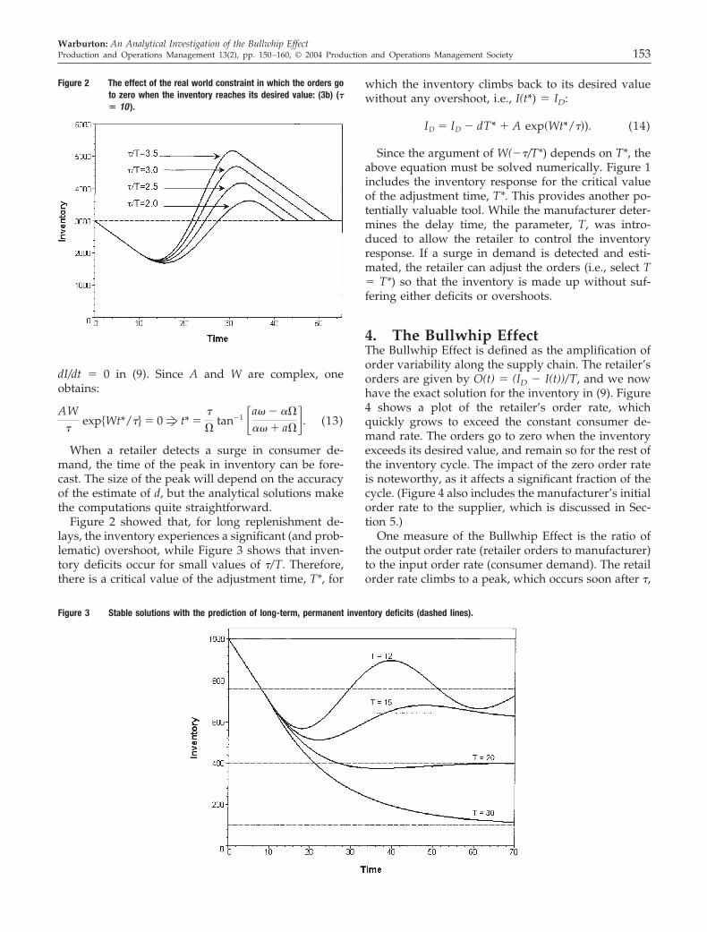
2.2. Inventory CyclesWe next demonstrate the importance of the real worldconstraint that the orders should go to zero when theinventory exceeds the desired value, (3b). The time at

which the inventory returns to its desired value, ID, isdefined as D. At D, the order rate goes to zero, butitems continue arriving, because there are still ordersin the pipeline. The inventory overshoots and it takesa further time, �, the replenishment time, until thepipeline empties. After t � TD � �, only the continuingconsumer demand remains, and so (6) applies again.When the inventory falls to its desired level, the cyclerepeats. The different characteristics of Figures 1 and 2are due to the orders stopping when the inventoryreaches its desired value.

2.3. Permanent Inventory DeficitsThe theoretical solution in the stable regime predictspermanent inventory deficits. When �/T � �/2, the realpart of W(z) is negative, and for large t, therefore, (9)becomes:

I�t 3 �� 3 ID � Td. (12)

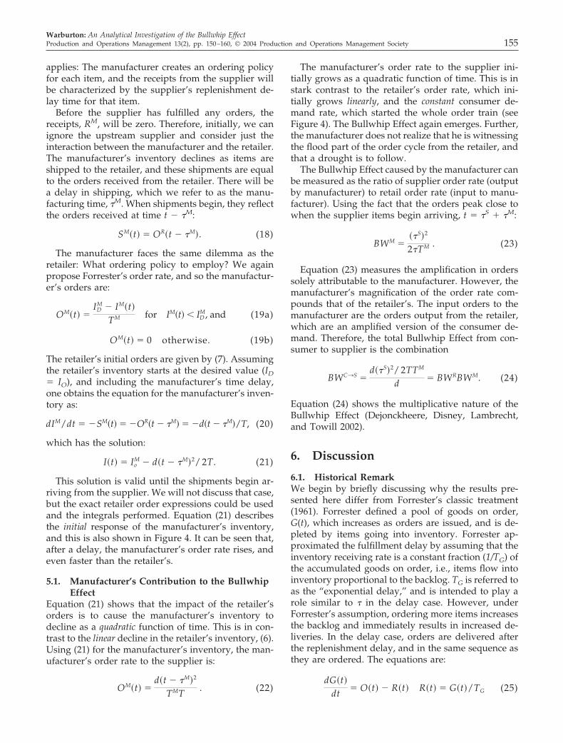
The inventory falls to a value permanently below itsdesired value by Td. Using the Final Value Theorem,John, Naim, and Towill (1994) proved analytically thatpermanent deficits occur. Figure 3 shows solutions inthis stable regime, which approach the predicted long-term deficits (dashed lines). For small z � �1/e, W(z)is real, and the solutions no longer oscillate, which canbe seen in Figure 3, where the curve for T � 30 showsno oscillation.

3. Managing the InventoryHaving derived the analytical solutions, we brieflyexplore some properties that will be useful when wediscuss the Bullwhip Effect. The time of the inventorypeak, referred to as t*, can be calculated by setting

Figure 1 Four exact solutions of the inventory equation. T* is the criticaladjustment rate, which brings the inventory exactly back to itsdesired value (� � 10 ).

Warburton: An Analytical Investigation of the Bullwhip Effect152 Production and Operations Management 13(2), pp. 150–160, © 2004 Production and Operations Management Society

dI/dt � 0 in (9). Since A and W are complex, oneobtains:

AW�

exp Wt*/�� 0f t* ��

tan�1 �a� �

� � a�. (13)

When a retailer detects a surge in consumer de-mand, the time of the peak in inventory can be fore-cast. The size of the peak will depend on the accuracyof the estimate of d, but the analytical solutions makethe computations quite straightforward.

Figure 2 showed that, for long replenishment de-lays, the inventory experiences a significant (and prob-lematic) overshoot, while Figure 3 shows that inven-tory deficits occur for small values of �/T. Therefore,there is a critical value of the adjustment time, T*, for

which the inventory climbs back to its desired valuewithout any overshoot, i.e., I(t*) � ID:

ID � ID � dT* � A exp�Wt*/��). (14)

Since the argument of W(��/T*) depends on T*, theabove equation must be solved numerically. Figure 1includes the inventory response for the critical valueof the adjustment time, T*. This provides another po-tentially valuable tool. While the manufacturer deter-mines the delay time, the parameter, T, was intro-duced to allow the retailer to control the inventoryresponse. If a surge in demand is detected and esti-mated, the retailer can adjust the orders (i.e., select T� T*) so that the inventory is made up without suf-fering either deficits or overshoots.

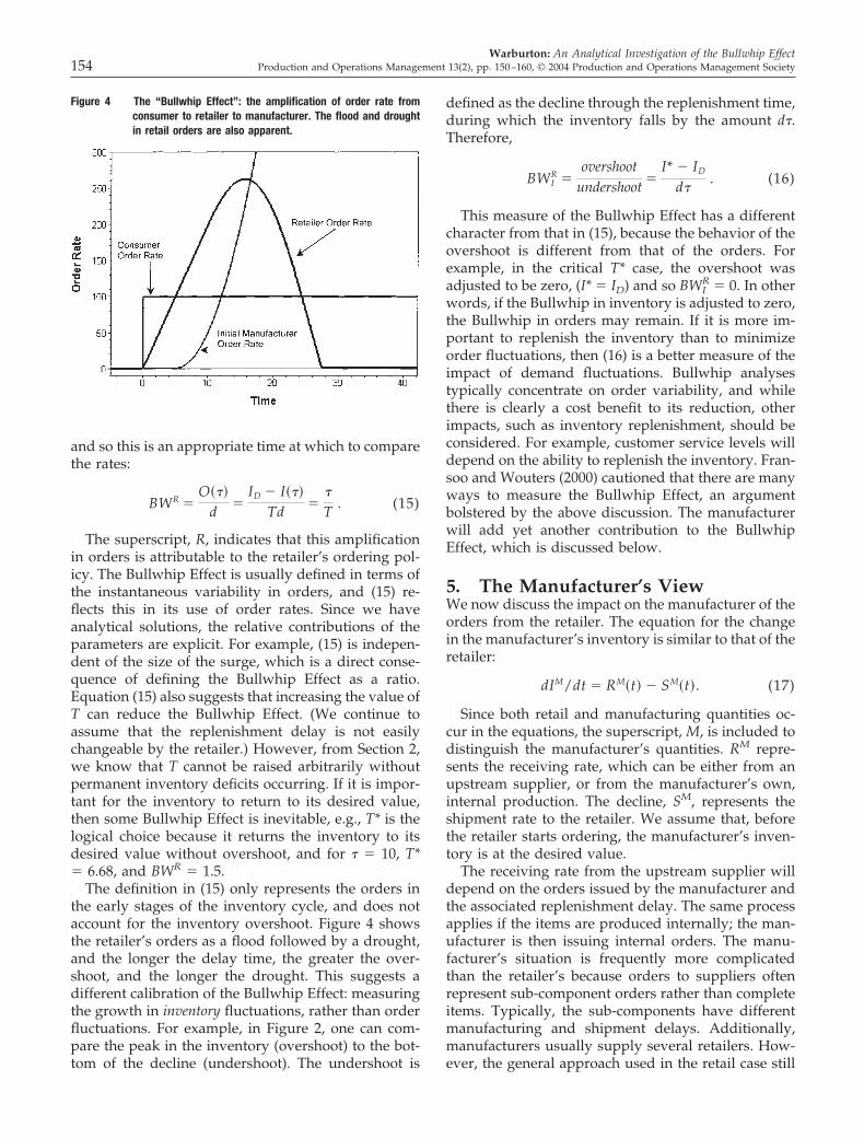
4. The Bullwhip EffectThe Bullwhip Effect is defined as the amplification oforder variability along the supply chain. The retailer’sorders are given by O(t) � (ID � I(t))/T, and we nowhave the exact solution for the inventory in (9). Figure4 shows a plot of the retailer’s order rate, whichquickly grows to exceed the constant consumer de-mand rate. The orders go to zero when the inventoryexceeds its desired value, and remain so for the rest ofthe inventory cycle. The impact of the zero order rateis noteworthy, as it affects a significant fraction of thecycle. (Figure 4 also includes the manufacturer’s initialorder rate to the supplier, which is discussed in Sec-tion 5.)

One measure of the Bullwhip Effect is the ratio ofthe output order rate (retailer orders to manufacturer)to the input order rate (consumer demand). The retailorder rate climbs to a peak, which occurs soon after �,

Figure 2 The effect of the real world constraint in which the orders goto zero when the inventory reaches its desired value: (3b) (�� 10 ).

Figure 3 Stable solutions with the prediction of long-term, permanent inventory deficits (dashed lines).


and so this is an appropriate time at which to comparethe rates:

BWR �O��

d �ID � I��

Td ��

T . (15)

The superscript, R, indicates that this amplificationin orders is attributable to the retailer’s ordering pol-icy. The Bullwhip Effect is usually defined in terms ofthe instantaneous variability in orders, and (15) re-flects this in its use of order rates. Since we haveanalytical solutions, the relative contributions of theparameters are explicit. For example, (15) is indepen-dent of the size of the surge, which is a direct conse-quence of defining the Bullwhip Effect as a ratio.Equation (15) also suggests that increasing the value ofT can reduce the Bullwhip Effect. (We continue toassume that the replenishment delay is not easilychangeable by the retailer.) However, from Section 2,we know that T cannot be raised arbitrarily withoutpermanent inventory deficits occurring. If it is impor-tant for the inventory to return to its desired value,then some Bullwhip Effect is inevitable, e.g., T* is thelogical choice because it returns the inventory to itsdesired value without overshoot, and for � � 10, T*� 6.68, and BWR � 1.5.

The definition in (15) only represents the orders inthe early stages of the inventory cycle, and does notaccount for the inventory overshoot. Figure 4 showsthe retailer’s orders as a flood followed by a drought,and the longer the delay time, the greater the over-shoot, and the longer the drought. This suggests adifferent calibration of the Bullwhip Effect: measuringthe growth in inventory fluctuations, rather than orderfluctuations. For example, in Figure 2, one can com-pare the peak in the inventory (overshoot) to the bot-tom of the decline (undershoot). The undershoot is

defined as the decline through the replenishment time,during which the inventory falls by the amount d�.Therefore,

BWIR �

overshootundershoot �

I* � ID

d�. (16)

This measure of the Bullwhip Effect has a differentcharacter from that in (15), because the behavior of theovershoot is different from that of the orders. Forexample, in the critical T* case, the overshoot wasadjusted to be zero, (I* � ID) and so BWI

R � 0. In otherwords, if the Bullwhip in inventory is adjusted to zero,the Bullwhip in orders may remain. If it is more im-portant to replenish the inventory than to minimizeorder fluctuations, then (16) is a better measure of theimpact of demand fluctuations. Bullwhip analysestypically concentrate on order variability, and whilethere is clearly a cost benefit to its reduction, otherimpacts, such as inventory replenishment, should beconsidered. For example, customer service levels willdepend on the ability to replenish the inventory. Fran-soo and Wouters (2000) cautioned that there are manyways to measure the Bullwhip Effect, an argumentbolstered by the above discussion. The manufacturerwill add yet another contribution to the BullwhipEffect, which is discussed below.

5. The Manufacturer’s ViewWe now discuss the impact on the manufacturer of theorders from the retailer. The equation for the changein the manufacturer’s inventory is similar to that of theretailer:

dIM/dt � RM�t� � SM�t�. (17)

Since both retail and manufacturing quantities oc-cur in the equations, the superscript, M, is included todistinguish the manufacturer’s quantities. RM repre-sents the receiving rate, which can be either from anupstream supplier, or from the manufacturer’s own,internal production. The decline, SM, represents theshipment rate to the retailer. We assume that, beforethe retailer starts ordering, the manufacturer’s inven-tory is at the desired value.

The receiving rate from the upstream supplier willdepend on the orders issued by the manufacturer andthe associated replenishment delay. The same processapplies if the items are produced internally; the man-ufacturer is then issuing internal orders. The manu-facturer’s situation is frequently more complicatedthan the retailer’s because orders to suppliers oftenrepresent sub-component orders rather than completeitems. Typically, the sub-components have differentmanufacturing and shipment delays. Additionally,manufacturers usually supply several retailers. How-ever, the general approach used in the retail case still

Figure 4 The “Bullwhip Effect”: the amplification of order rate fromconsumer to retailer to manufacturer. The flood and droughtin retail orders are also apparent.


applies: The manufacturer creates an ordering policyfor each item, and the receipts from the supplier willbe characterized by the supplier’s replenishment de-lay time for that item.

Before the supplier has fulfilled any orders, thereceipts, RM, will be zero. Therefore, initially, we canignore the upstream supplier and consider just theinteraction between the manufacturer and the retailer.The manufacturer’s inventory declines as items areshipped to the retailer, and these shipments are equalto the orders received from the retailer. There will bea delay in shipping, which we refer to as the manu-facturing time, �M. When shipments begin, they reflectthe orders received at time t � �M:

SM�t� � OR�t � �M�. (18)

The manufacturer faces the same dilemma as theretailer: What ordering policy to employ? We againpropose Forrester’s order rate, and so the manufactur-er’s orders are:

OM�t� �ID

M � IM�t�TM for IM�t� � ID

M, and (19a)

OM�t� � 0 otherwise. (19b)

The retailer’s initial orders are given by (7). Assumingthe retailer’s inventory starts at the desired value (ID

� IO), and including the manufacturer’s time delay,one obtains the equation for the manufacturer’s inven-tory as:

dIM/dt � �SM�t� � �OR�t � �M� � �d�t � �M�/T, (20)

which has the solution:

I�t� � IoM � d�t � �M�2/ 2T. (21)

This solution is valid until the shipments begin ar-riving from the supplier. We will not discuss that case,but the exact retailer order expressions could be usedand the integrals performed. Equation (21) describesthe initial response of the manufacturer’s inventory,and this is also shown in Figure 4. It can be seen that,after a delay, the manufacturer’s order rate rises, andeven faster than the retailer’s.

5.1. Manufacturer’s Contribution to the BullwhipEffect

Equation (21) shows that the impact of the retailer’sorders is to cause the manufacturer’s inventory todecline as a quadratic function of time. This is in con-trast to the linear decline in the retailer’s inventory, (6).Using (21) for the manufacturer’s inventory, the man-ufacturer’s order rate to the supplier is:

OM�t� �d�t � �M�2

TMT . (22)

The manufacturer’s order rate to the supplier ini-tially grows as a quadratic function of time. This is instark contrast to the retailer’s order rate, which ini-tially grows linearly, and the constant consumer de-mand rate, which started the whole order train (seeFigure 4). The Bullwhip Effect again emerges. Further,the manufacturer does not realize that he is witnessingthe flood part of the order cycle from the retailer, andthat a drought is to follow.

The Bullwhip Effect caused by the manufacturer canbe measured as the ratio of supplier order rate (outputby manufacturer) to retail order rate (input to manu-facturer). Using the fact that the orders peak close towhen the supplier items begin arriving, t � �S � �M:

BWM ��S�2

2�TM . (23)

Equation (23) measures the amplification in orderssolely attributable to the manufacturer. However, themanufacturer’s magnification of the order rate com-pounds that of the retailer’s. The input orders to themanufacturer are the orders output from the retailer,which are an amplified version of the consumer de-mand. Therefore, the total Bullwhip Effect from con-sumer to supplier is the combination

BWC3S �d��S�2/ 2TTM

d � BWRBWM. (24)

Equation (24) shows the multiplicative nature of theBullwhip Effect (Dejonckheere, Disney, Lambrecht,and Towill 2002).

6. Discussion

6.1. Historical RemarkWe begin by briefly discussing why the results pre-sented here differ from Forrester’s classic treatment(1961). Forrester defined a pool of goods on order,G(t), which increases as orders are issued, and is de-pleted by items going into inventory. Forrester ap-proximated the fulfillment delay by assuming that theinventory receiving rate is a constant fraction (1/TG) ofthe accumulated goods on order, i.e., items flow intoinventory proportional to the backlog. TG is referred toas the “exponential delay,” and is intended to play arole similar to � in the delay case. However, underForrester’s assumption, ordering more items increasesthe backlog and immediately results in increased de-liveries. In the delay case, orders are delivered afterthe replenishment delay, and in the same sequence asthey are ordered. The equations are:

dG�t�dt � O�t� � R�t� R�t� � G�t�/TG (25)


The order rate is again given by Forrester’s expres-sion, (3a), which results in an ordinary, second orderdifferential equation for the inventory:

I� � I�/TG � I�/TG T � ID /TG T. (26)

Forrester ignored the real world constraint in whichthe order rate goes to zero when the inventory exceedsits desired value. The solution to (26) is:

I � ID � exp�t��A sin � t� � B cos � t��. (27)

Substitution into the homogeneous equation deter-mines the constants and , while the boundaryconditions (G(0) � Go and dI/dt � Go/TG) determinethe constants A and B:

� �1/�2TG� 2 �1

TGT �1 �T

4TG�

A �Go

TG�

�Io � ID�

B � Io � ID. (28)

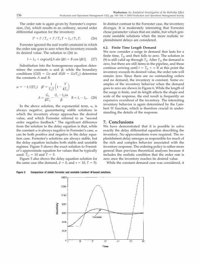
In the above solution, the exponential term, , isalways negative, guaranteeing stable solutions inwhich the inventory always approaches the desiredvalue, and which Forrester referred to as “secondorder negative feedback.” The significant differencefrom the solution to the delay equation is that, whilethe constant is always negative in Forrester’s case, �can be both positive and negative in the delay equa-tion case. Forrester’s solutions are always stable, butthe delay equation includes both stable and unstableregimes. Figure 5 shows the exact solution to Forrest-er’s approximate equation for values that he typicallyused: TG � 10 and T � 5.

Figure 5 also shows the delay equation solution forthe same case (the demand, d � 0, and � � 10, T � 5).

In distinct contrast to the Forrester case, the inventorydiverges. It is moderately interesting that Forresterchose parameter values that are stable, but which gen-erate unstable solutions when the more realistic re-plenishment delays are considered.

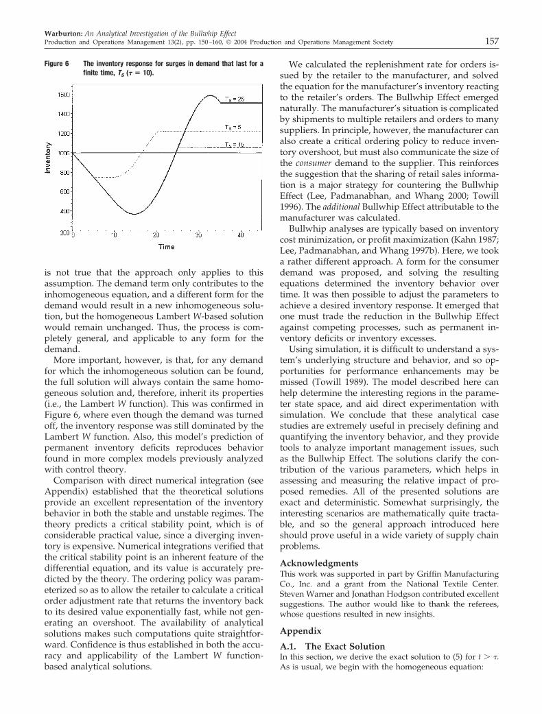
6.2. Finite Time Length DemandWe now consider a surge in demand that lasts for afinite time, TS, and then falls to zero. The solution in(9) is still valid up through TS. After TS, the demand iszero, but there are still items in the pipeline, and thesecontinue arriving until t � TS � �. If at this point theinventory exceeds its desired value, the order rate willremain zero. Since there are no outstanding ordersand no demand, the inventory is constant. Some ex-amples of the inventory behavior when the demandgoes to zero are shown in Figure 6. While the length ofthe surge is finite, and its length affects the shape andscale of the response, the end result is frequently anexpensive overshoot of the inventory. The interestinginventory behavior is again determined by the Lam-bert W function, which is therefore crucial in under-standing the details of the response.

7. ConclusionsWe have demonstrated that it is possible to solveexactly the delay differential equation describing theinventory. No approximations were required. The re-plenishment delay emerges as responsible for much ofthe rich and complex behavior associated with theinventory response. The ordering policy is rather moregeneral than previous theoretical analyses because itincludes the realistic condition that the order rate iszero once the inventory reaches its desired value.

While the constant demand case was considered, it

Figure 5 Comparison of stable Forrester and unstable Lambert W-based solutions.


is not true that the approach only applies to thisassumption. The demand term only contributes to theinhomogeneous equation, and a different form for thedemand would result in a new inhomogeneous solu-tion, but the homogeneous Lambert W-based solutionwould remain unchanged. Thus, the process is com-pletely general, and applicable to any form for thedemand.

More important, however, is that, for any demandfor which the inhomogeneous solution can be found,the full solution will always contain the same homo-geneous solution and, therefore, inherit its properties(i.e., the Lambert W function). This was confirmed inFigure 6, where even though the demand was turnedoff, the inventory response was still dominated by theLambert W function. Also, this model’s prediction ofpermanent inventory deficits reproduces behaviorfound in more complex models previously analyzedwith control theory.

Comparison with direct numerical integration (seeAppendix) established that the theoretical solutionsprovide an excellent representation of the inventorybehavior in both the stable and unstable regimes. Thetheory predicts a critical stability point, which is ofconsiderable practical value, since a diverging inven-tory is expensive. Numerical integrations verified thatthe critical stability point is an inherent feature of thedifferential equation, and its value is accurately pre-dicted by the theory. The ordering policy was param-eterized so as to allow the retailer to calculate a criticalorder adjustment rate that returns the inventory backto its desired value exponentially fast, while not gen-erating an overshoot. The availability of analyticalsolutions makes such computations quite straightfor-ward. Confidence is thus established in both the accu-racy and applicability of the Lambert W function-based analytical solutions.

We calculated the replenishment rate for orders is-sued by the retailer to the manufacturer, and solvedthe equation for the manufacturer’s inventory reactingto the retailer’s orders. The Bullwhip Effect emergednaturally. The manufacturer’s situation is complicatedby shipments to multiple retailers and orders to manysuppliers. In principle, however, the manufacturer canalso create a critical ordering policy to reduce inven-tory overshoot, but must also communicate the size ofthe consumer demand to the supplier. This reinforcesthe suggestion that the sharing of retail sales informa-tion is a major strategy for countering the BullwhipEffect (Lee, Padmanabhan, and Whang 2000; Towill1996). The additional Bullwhip Effect attributable to themanufacturer was calculated.

Bullwhip analyses are typically based on inventorycost minimization, or profit maximization (Kahn 1987;Lee, Padmanabhan, and Whang 1997b). Here, we tooka rather different approach. A form for the consumerdemand was proposed, and solving the resultingequations determined the inventory behavior overtime. It was then possible to adjust the parameters toachieve a desired inventory response. It emerged thatone must trade the reduction in the Bullwhip Effectagainst competing processes, such as permanent in-ventory deficits or inventory excesses.

Using simulation, it is difficult to understand a sys-tem’s underlying structure and behavior, and so op-portunities for performance enhancements may bemissed (Towill 1989). The model described here canhelp determine the interesting regions in the parame-ter state space, and aid direct experimentation withsimulation. We conclude that these analytical casestudies are extremely useful in precisely defining andquantifying the inventory behavior, and they providetools to analyze important management issues, suchas the Bullwhip Effect. The solutions clarify the con-tribution of the various parameters, which helps inassessing and measuring the relative impact of pro-posed remedies. All of the presented solutions areexact and deterministic. Somewhat surprisingly, theinteresting scenarios are mathematically quite tracta-ble, and so the general approach introduced hereshould prove useful in a wide variety of supply chainproblems.

AcknowledgmentsThis work was supported in part by Griffin ManufacturingCo., Inc. and a grant from the National Textile Center.Steven Warner and Jonathan Hodgson contributed excellentsuggestions. The author would like to thank the referees,whose questions resulted in new insights.

Appendix

A.1. The Exact SolutionIn this section, we derive the exact solution to (5) for t � �.As is usual, we begin with the homogeneous equation:

Figure 6 The inventory response for surges in demand that last for afinite time, TS (� � 10).


dIdt

�I�t � ��

T� 0. (A.1)

The complexity of this equation is associated with thereplenishment delay. The equation is referred to as the lo-gistics equation, and is a member of the class of delaydifferential equations (Bellman and Cooke 1963). We pro-pose a solution of the form I � A exp(st), to obtain:

Aest s � e�s�/T� � 0. (A.2)

The term in braces can be rearranged into the followingsuggestive form:

s�es� � ��/T. (A.3)

Equation (A.3) can be solved exactly in terms of the LambertW function, which is defined as:

W� z�eW� z� � z. (A.4)

A review of the history, theory, and applications of theLambert W function may be found in Corless et al. (1996).There are an infinite number of complex values of the Lam-bert W function, denoted as W(k, z). By the linearity of (A.1),any combination of the W(k, z) can be used in the solution,and we could consider a solution of the form:

I�t� � �k

ck exp�W�k, ��/T�t/��. (A.5)

This is an infinite formula and we are interested in prac-tical, easy-to-implement solutions. It turns out that usingjust the first term (k � 0) results in a sufficiently accuraterepresentation of the inventory response. Therefore, our“practical” solution is:

I�t� � A exp�Wt/�� with W � W�0, ��/T�. (A.6)

The inventory behavior is extremely sensitive to the prop-erties of W(z), because it occurs in the exponential. Fortu-nately, the Lambert W function is readily available in effi-cient and accurate implementations, such as in MAPLE(2002), where it is defined as Lambert W(k, z). W(z) onlyenters (A.6) as a parameter; there is no time dependence inthe W(z) term.

We now proceed to solve the inhomogeneous equation.The inhomogeneous term is a constant, so we propose theconstant, K, as a solution. Substitution in (5) determines K asK � ID � dT. Adding this to the homogeneous solutiongives:

I�t� � ID � dT � A exp�Wt/��. (A.7)

The constant, A, is determined by the imposition ofboundary conditions. The inventory must be continuous,and so (A.7) must match the solution in (6) at t � �. In orderto guarantee appropriate behavior at t � �, it is also neces-sary to specify the slope of the inventory there, and (2)provides the required condition. Two conditions on theinventory require two integration constants. Noting that Wis complex suggests that A can be also. Treating A as acomplex constant results in a solution that turns out toprovide an excellent representation of the inventory over theentire range of �/T. Therefore, we consider A and W as:

A � a � i W � � � i. (A.8)

Matching the solution in (6) to that of (A.7) at t � �, gives:

a cos � sin � e��Io � ID � d�T � ��. (A.9)

Differentiating (A.7) at t � �, gives the required condition onthe derivative:

dIdt� t��

� R�� d � O�0� � d

�ID � Io

T� d �

AW�

eW. (A.10)

This provides a second relation between a and , whichcan thus be determined in terms of � and . The complete,exact solution to (5) is thus determined, and is given in (9).

A number of combinations of solutions from (A.5) weretried. Despite adding complexity, including more LambertW functions, doesn’t significantly improve the match to thenumerical solution. Considering the constant, A, as complex,provides two parameters, and guarantees the continuity ofthe solution and its derivative at t � �. From a practicalperspective, once the inventory climbs back to ID, (3b) ap-plies, and the solution changes. In practice, therefore, theLambert W function is only required until I � ID. We con-clude that the k � 0 term with a complex constant providesa practical representation of the inventory behavior in boththe stable and unstable regimes.

A.2. The Accuracy of the Theoretical SolutionThe above discussion suggests that only the first term in theseries in (A.5) is required, and we now examine the accuracyof that assumption. Figure 7 compares the analytical solu-tions with numerical integrations of the same differentialequation. The difference between the theoretical and numer-ical solutions in the unstable regime is less than 3% at thefirst peak. In the stable regime, there is very little differencebetween the theoretical and numerical solutions. The theo-retical solution also predicts the period of oscillation tobetter than 0.4%. Therefore, in practical situations wherethere is likely to be noise in the data, the one-term LambertW function provides an easy-to-compute, accurate represen-tation of the inventory response.

A.3. The Impact of the Lambert W FunctionThe properties of the solutions are determined by the char-acteristics of the Lambert W function. For large �/T, the realpart of the Lambert function, �, is positive and the solutionsdiverge (Figure 1). However, for small values of �/T � �,W(��) � ��, which is real, and results in stable, decayingsolutions. The issue is to determine the critical stabilitypoint. There are two interesting values for the argument ofW(z), �1/e and ��/2.

When �/T � �/2, the real part of W(z) is positive, and thesolution in (9) applies. The oscillation is due to the imagi-nary part of the Lambert function, . As �/T increases, increases, resulting in a decrease in the period, which can beclearly seen in Figure 1.

The real part of W(z) � 0 at ��/2. Therefore, the transitionfrom unstable to stable solutions occurs when �/T � �/2. Adetailed numerical integration of the delay equation was


performed on either side of the critical stability value (�� 10.0f T � 6.36 � 0.1). One slowly diverged and the otherslowly converged, validating that the critical stability pointis in fact an inherent feature of the differential equation. Theability to predict this critical stability point is very valuable,because it divides stable from unstable inventory behavior.

A.4. Analysis of AssumptionsWhile we considered the constant demand case, it is not truethat the solution only applies to this assumption. Since (5) islinear, its solution is always the sum of homogeneous andinhomogeneous components. A different demand wouldresult in a new inhomogeneous component, but the homo-geneous Lambert W-based component would remain un-changed. Therefore, the process is completely general andapplicable to any form for the demand.

The analytical solutions reproduced the inventory def-icit prediction of control theory, and we can hypothesizeas to why the simplified model (without a WIP term)includes such behavior found in more complex models.The critical stability point and other interesting character-istics are properties of the exponential Lambert W func-tion, which arises from the solution to the homogeneousequation. Therefore, any system of equations that in-cludes the replenishment delay (a homogeneous term)should inherit these characteristics. In contrast, the de-mand leads to inhomogeneous terms, e.g., d is on theright-hand side of (5). As long as the ordering policyincludes a time delay in fulfillment, adding WIP termsshould merely add inhomogeneous terms to the homoge-neous Lambert W solutions. We tentatively concludethat it is reasonable to expect more complex models toinherit the properties described here. In which case, de-spite its apparent simplicity, the present model has sig-nificant predictive power, and is of considerable theoret-ical interest. Further research is underway to confirm thisconjecture.

ReferencesAnderson Jr., E. G., D. J. Morrice. 2000. A simulation game for

service-oriented supply chain management: Does informationsharing help managers with service capacity decisions? Produc-tion and Operations Management 9(1) 40–55.

Anderson Jr., E. G., C. H. Fine, G. G. Parker. 2000. Upstreamvolatility in the supply chain: The machine tool industry as acase study. Production and Operations Management 9(3) 239–261.

Bellman, R. E., K. L. Cooke. 1963. Differential-difference equations.Academic Press, New York.

Berry, D., D. R. Towill. 1995. Reduce costs: Use a more intelligentproduction and inventory policy. BPICS Control Journal 1(7)26–30.

Bourland, K., S. Powell, D. Pyke. 1996. Exploring timely demandinformation to reduce inventories. European Journal of Opera-tions Research 92 239–253.

Burbidge, J. L. 1961. The “new approach” to production. ProductionEngineer 40 3–19.

Burbidge, J. L. 1984. Automated production control with a simula-tion capability. Proceedings of IFIP Conference WG 5–7, Copen-hagen, 1–14.

Buzzell, R. D., J. A. Quelch, W. J. Salmon. 1990. The costly bargainof trade promotion. Harvard Business Review 68(March April)141–148.

Clark, T. 1994. Campbell Soup: A leader in continuous replenish-ment innovations. Harvard Business School Case, Boston, Massa-chusetts.

Corless, R. M., G. H. Gonnet, D. E. G. Hare, D. J. Jeffrey, D. E. Knuth.1996. On the Lambert W function. Advances in ComputationalMathematics 5 329–359.

Dejonckheere, J., S. M. Disney, M. R. Lambrecht, D. R. Towill. 2002.Transfer function analysis of forecasting induced bullwhip insupply chains. International Journal of Production Economics 78133–144.

Disney, S. M., M. M. Naim, D. R. Towill. 2000. Genetic algorithmoptimization of a class of inventory control systems. Interna-tional Journal of Production Economics 68 259–278.

Disney, S. M., D. R. Towill. 2002a. Inventory drift and instability in

Figure 7 Comparison of theoretical and numerical solutions, showing differences of less than 3% (at the peak) in the unstable regime, and smalldifferences in the stable regime (� � 10 ).


order-up-to replenishment policies. Proceedings of the 12th Inter-national Symposium on Inventories, August, Budapest, Hungary.

Disney, S. M., D. R. Towill. 2002b. A discrete transfer functionmodel to determine the dynamic stability of a vendor managedinventory supply chain. International Journal of Production Re-search 40(1) 179–204.

Disney, S. M., D. R. Towill. 2002c. A procedure for the optimizationof the dynamic response of a vendor managed inventory sys-tem. Computers and Industrial Engineering 43 27–58.

Fine, C. 2000. Clockspeed-based strategies for supply chain design.Production and Operations Management 9(3) 213–221.

Forrester, J. W., 1961. Industrial Dynamics, MIT Press, Cambridge,Massachusetts.

Fransoo, M., J. F. Wouters. 2000. Measuring the bullwhip effect inthe supply chain. Supply Chain Management 5(2) 78.

Gavirneni, S., R. Kapuscinski, S. Tayur. 1999. Value of informationin capacitated supply chains. Management Science 45(1) 16–24.

Gill, P., J. Abend. 1997. Wal-Mart: The supply chain heavyweightchamp. Supply Chain Management Review 1(1) 8–16.

Hammond, J. 1993. Quick response in retail/manufacturing chan-nels in Globalization, technology and competition: The fusion ofcomputers and telecommunication in the 1990’s, Bradley et al. (ed.),Harvard Business School Press, Boston, Massachusetts, 185–214.

Holmstrom, J. 1997. Product range management: a case study ofsupply chain operations in the European grocery industry.Supply Chain Management 2(3) 107–115.

John, S., M. M. Naim, D. R. Towill. 1994. Dynamic analysis of a WIPcompensated decision support system. International Journal ofManufacturing Design 1(4) 283–297.

Johnson, M. E., S. Whang. 2002. E-business and supply chain man-agement: An overview and framework. Production and Opera-tions Management 11(4) 413–423.

Kahn, J. 1987. Inventories and the volatility of production. AmericanEconomic Review 77 667–679.

Kelly, K. 1995. Burned by busy signals: Why Motorola ramped upproduction way past demand. Business Week 6 36.

Lee, H. L., V. Padmanabhan, S. Whang. 1997a. Information distor-tion in the supply chain: The Bullwhip Effect. ManagementScience 43(4) 546–558.

Lee, H. L., V. Padmanabhan, S. Whang. 1997b. The bullwhip effectin supply chains. Sloan Management Review 38(3) 93–102.

Lee, H. L., K. C. So, C. S. Tang. 2000. The value of informationsharing in a two-level supply chain. Management Science 46(5)626–643.

MAPLE. 2002. Computer Program, Version 8. Waterloo Maple, Inc.,Ontario, Canada.

Metters, R. 1997. Quantifying the bullwhip effect in supply chains.Journal of Operations Management, Columbia, May.

Sterman, J. D. 1989. Modeling managerial behavior: Misperceptionsof feedback in a dynamic decision-making experiment. Man-agement Science 35(3) 321–339.

Towill, D. 1989. The dynamic analysis approach to manufacturingsystems design. Journal of Advanced Management Engineering 1131–140.

Towill, D. 1996. Time compression and the supply chain: A guidedtour. Supply Chain Management 1(1) 15–27.

Towill, D. 1997. FORRIDGE: Principles of good practice in materialflow. Production Planning and Control 8(7) 622–632.


Documents

An Analytical Investigation of the Bullwhip Effect