\AN APPLICATION OF RELAXATION METHODS

TO

TRANSONIC NOZZLE FLO~

by

Kevin Eugene ~Walsh/,>

Thesis submitted to the Graduate Faculty of the

Virginia Polytechnic Institute and State University

in partial fulfillment of the requirements for the degree of

MASTER OF SCIENCE

in

Mechanical Engineering

APPROVED:

}fled '-«' , F, O'Brien '7

September, 1974

Blacksburg, Virginia

LD 5G55 Y<655 I q7Jf W37 (}, ~

ACKNOWLEDGEMENTS

This work was funded by the Douglas Aircraft Company, McDonnell

Douglas Corporation, under a research contract. I would like to thank

the secretarial staff of the Mechanical Engineering Department for

typing the manuscript and the Graphic Arts Department of the University's

Media Services for preparing the figures. Thanks are also due

Professors Walter F. O'Brien and George W. Swift for their help in

course and administrative work over the past year. But I am especially

grateful to my advisor, Dr. Eugene F. Brown, whose encouragement and

insight are responsible for the successful results obtained.

ii

TABLE OF CONTENTS

Page

1. Introduction ............................................... 1

1.1 Problem Description 1

1.2 The Need for Numerical Relaxation 2

2. Literature Review •••••••••••••••••••••••••••••••••••••••••••••• 5

2.1 Solution of Transonic Small Perturbation Equation 5

2.2 Solution of Euler's Equations 8

2.3 A Comment on Relaxation Factors and Convergence ••••••••••• 11

3. Method Des cription ••••••••••••••••••••••••••••••••••••••••••••• 13

3.1 Governing Equations ••••••••••••••••••••••••••••••••••••••• 13

3.2 Coordinate Transformation ................................. 14

3.3 Finite-Difference Approximation . . . . . . . . . . . . . . . . . . . . . . .. 17

3.4 Boundary Conditions ••••••••••••••••••••••••••••••••••••••• 18

3.5 Relaxation Process •••. 21

4. Results and Discussion ••••••••••••••••••••••••••••••••••••••••• 24

5. Conclusions. • • • • • • • • • • • • • • • • • • • • • • • • • • • • • • • • • • • • • • • • • • • • • • • • • •• 33

6. Appendix. . . . . . . . . . . . . . . . . . . . . . . . . . . . . . . . . . . . . . . . . . . . . . . . . . . . . .. 34

6.1 Derivation of the Column Matrix Form of the Governing Equation ••••••••••••••••••••••••••••••••• 34

6.2 Flow Chart of Relaxation Program ••• 37

7. References ••••••••••••••••••••••••••••••••••••••••••••••••••••• 42

8. Vita ............................•.............................. 44

iii

LIST OF FIGURES

Figure No. Title Page

1 Coordinate Transformation •••••••••••••••••••••••• 15

2 Finite-Difference Molecules •••••••••••••••••••••• 19

3 Test-Case Nozzle Geometry •••••••••••••••••••••••• 25

4 Lines of Constant Mach Number •••••••••••••••••••• 26

5 Change of Mach Number at Various Nozzle Locations with Number of Iterations •••••••••••••• 27

6 Discharge Coefficient •••••••••••••••••••••••••••• 29

7 Effect of Boundary Treatment and Finite-Difference Form on Relaxation Solution ••••••••••• 31

iv

A., B., C

A

c

c

CD

Cv D

f

K

L

M

m

n

p

Pb

r

R

T

u

v

V

x

LIST OF SYMBOLS

Coefficients of the second derivatives in the governing equation

Coefficient matrix of governing equation in tridiagonal form

Speed of sound

c/c o

Discharge coefficient

Velocity coefficient

Non-homogeneous term in tridiagonal form of governing equation

Non-homogeneous vector in tridiagonal form of governing equation

Transonic similarity parameter

Total length of constant-area section and nozzle

Mach number

Mass flow rate

Number of iterations

Pressure

Nozzle back pressure

Radial coordinate in the physical plane

Nozzle wall radius

Thrust

Axial velocity component

Radial velocity component

Velocity

Axial coordinate in the physical plane

v

w

Subscripts

a

e

id

i

I

j

J

o

vi

Lateral coordinate in the physical plane (for planar flow)

Ratio of specific heats

Mesh spacing in axial direction (physical plane)

Mesh spacing in radial direction (physical plane)

Mesh spacing in axial direction (computational plane)

Mesh spacing in radial direction (computational plane)

Flow angle

Nozzle wall angle

Axial coordinate in the computational plane

Density

Velocity potential function

Non-dimensionalized potential function

Column vector of unknown ~'s

Radial coordinate in the computational plane

Steam function

Relaxation factor

Actual

Refers to nozzle exit

Ideal

Mesh point index in the axial direction

Largest axial index

Mesh point index in the radial direction

Largest radial index

Stagnation conditions

r

th

W

x

~

1P

Superscripts

*

vii

Radial derivative in the physical plane

Refers to nozzle throat

Refers to nozzle wall

Axial derivative in the physical plane

Axial derivative in the computational plane

Radial derivative in the computational plane

Refers to sonic conditions

Average

Matrix or vector

1. INTRODUCTION

1.1 Problem Description

An exhaust nozzle is a critical component of any turbojet propulsion

system. Its purpose is to create thrust by accelerating exhaust gases

to a high velocity. In the exhaust nozzles found on today's turbojet

aircraft, velocities reach and exceed the speed of sound. Accurate

analytical methods capable of handling these transonic flows are required

for the design and development of new nozzle configurations. This is

underscored by studies of supersonic transport aircraft (1) which have

shown that errors of one percent in such operating characteristics as

the velocity coefficient result in errors in the predicted specific fuel

consumption of over two percent and errors in the operating cost

predictions of over three percent.

The desired nozzle performance data could be obtained analytically

by the solution of the Navier-Stokes equations. Although some progress

is today being made in their solution, the mathematical complexity of

these equations preclude their use in this study. Instead, the simpler

Euler's equations which assume inviscid flow were used. Adiabatic

flow was also assumed, giving isentropic flow. These assumptions were

justified by the simplicity of Euler's equations, the ability to

include viscous effects by means of boundary layer analysis once

Euler's equations are solved, and the fact that low Mach number shocks

(M ~ 1.3) cause negligible entropy changes.

-1-

-2-

Even Euler's equations, when further simplified by the assumption

of steady flow of a perfect gas, are presently without a closed-form,

analytical (as opposed to numerical) solution. The equations contain

second order partial derivatives and are only quasi-linear, or linear

in the highest order derivatives. An additional difficulty arises from

a change in equation type with the local Mach number, from elliptic

in subsonic flow to hyperbolic in supersonic flow. Any solution method,

therefore, must be capable of handling non-linear, partial differential

equations of mixed type.

1.2 The Need for Numerical Relaxation

In 150 years of transonic nozzle flow investigation, observers

have commented that as many solution methods have appeared as there

are problems and investigators in the field. These methods, however,

can be divided into two types, indirect and direct (1). In the indirect

methods a boundary geometry is calculated from a specified velocity

or pressure distribution, while in the direct methods a geometry is

specified and the characteristics of the resulting flow field are

calculated. Only direct methods will be considered here because in

most exhaust nozzle problems the boundary geometry is specified and

the resulting performance is desired. Direct methods can with a few

exceptions be divided into series expansion, time-dependent, and

relaxation methods. Of most current interest are the time-dependent and

relaxation methods which require the use of digital computers.

The series expansion methods make use of polynomial representations

of the dependent variables. The coefficients of these polynomials are

-3-

obtained from the specified nozzle geometry. Most of these methods use

the small perturbation form of the transonic flow equation, and thus the

results are restricted to nozzles with large radii of curvature. Further­

more the accuracy of the solution is reduced in regions away from the

nozzle throat. Even methods which use the full governing equations,

such as Oswatitsch and Rothstein (2), are limited in terms of the throat

radius of curvature. In addition, convergent nozzles cannot be handled

due to the required specification of boundary geometry (1).

In time-dependent methods, the difficulty introduced by the

equation being of a mixed type is overcome by the introduction of

unsteady, time-dependent terms which change the governing equation to

hyperbolic type independent of the local Mach number. The steady,

mixed-flow, boundary (elliptic) and initial value (hyperbolic) problem

is then solved as the asymptotic limit of an unsteady, initial value

problem. Unlike series expansion methods, time-dependent solutions have

been obtained for convergent nozzles, are accurate for very small radii

of curvature, and have shown promise in calculating shock and viscous

flows and flows with inlet non-uniformities (1). Disadvantages are

excessive computation time (1) and inaccuracy in the subsonic region (3).

Relaxation methods encompass the iterative techniques of Richardson,

Liebman (or Gauss and Seidel) and Southwell (as applied cyclically for

machine computation) (4). Stripped of modifications which increase the

rate of convergence, relaxation consists simply of obtaining successive

approximations to the solution of the finite-difference form of the

governing equations. The method as originally developed was applied

-4-

to the solution of elliptic, boundary value problems, but Murman and

Cole (5) determined that the use of backward differencing in forming

derivative approximations in hyperbolic (supersonic) regions would enable

relaxation to handle mixed-type problems. According to l1urman,

relaxation methods when thus modified are capable not only of handling

transonic flows, but of doing so at five to ten times the computational

speed of time-dependent methods with no loss in accuracy (6). A study

by Brown (1) comparing times for the two methods in terms of computation

time per point, normalized with respect to the same computer, shows

relaxation to be an order of magnitude faster than time-dependent

solutions. The computational efficienqy of relaxation methods has as

yet only been demonstrated for external flow problems such as airfoil

calculations; however, similar economy is expected for nozzle flow

problems. Because of this the relaxation method was chosen for use in

this investigation.

2. LITERATURE REVIEW

The papers on numerical relaxation related to transonic flows deal

almost exclusively with external flow, specifically flow about airfoils

and bodies of revolution such as cone-cylinder combinations. In a

later section the extension of these methods to the problem of transonic

nozzle flow 'viII be discussed.

2.1 Solution of Transonic Small Perturbation Equation

In his first paper with Cole (5) and in a later individual work (6),

Murman described the use of relaxation with a type-dependent, finite-

difference technique to solve the transonic small perturbation equation

which was written as

[K - (y + 1) 4> ] 4> + 4> = 0 x xx yy

where K is the transonic similarity parameter. The type-dependent

finite-difference technique had the purpose of maintaining the domain

of dependence of the differential equation in its finite-difference

representation by relating the finite-difference expressions to the

local Mach number.

In the subsonic (elliptic) region, a centered difference expression

was used for the derivatives in the flow direction (4)x and 4>xx) con­

sistent with the equation's domain of dependence which extends infinitely

far in all directions. In the supersonic (hyperbolic) region, however,

an upwind difference expression was used for these derivatives since

-5-

-6-

the domain of dependence extends only upstream, bounded by right and

left running characteristics. (This bounded domain of dependence in

supersonic flow is ~epresented physically as the well-known zones of

silence and action.) This retarded differencing, with either an

explicit formulation obeying the Courant-Friedrichs-Lewy criterion or

an implicit formulation, is necessary for stability in the supersonic

region. The centered difference is consistent with the domain of

dependence of the radial derivative ($ ) in both regions, since yy

a column of points is solved simultaneously.

Murman and Cole's centered differences were of second order

accuracy and used two mesh points for the first derivative and three

points for the second. Both first order accurate (two and three point)

and second order accurate (four point) backward differences were tried,

with the conclusion that the first order form gave more reliable

results. The algebraic equations obtained by the substitution of these

finite-difference expressions were solved column by column in the down-

stream direction by successive line relaxation using a tridiagonal

algorithm (7).

The small perturbation method of Murman and Cole was modified to

handle sonic mesh points by Murman and Krupp (8), to insure that

exactly sonic points resulted in hyperbolic equations. The method

was applied successfully to numerous external flow problems involving

airfoils and bodies of revolution by these investigators (9), and by

Bailey (10), Bailey and Ballhaus (11), Ballhaus and Bailey (12), and

Caughey (13). Bailey and Steger (14) used a combination of the potential

-7-

function and primitive velocity variable forms of the small

disturbance equation. All results agreed well with available

theoretical and experimental data.

Yoshihara (15) discussed the small disturbance procedure of

Murman and Cole in a general review of transonic computational methods.

He noted the possibility of a matching problem between flow types along

the sonic line in cases where the centered difference indicated a

supersonic point, but the backward difference resulted in a subsonic

velocity at the point. Yoshihara added that Krupp (16) arbitrarily

used a centered finite-difference in such cases, and that while such

a treatment has no physical or mathematical basis, it would have

significant consequences only when a shock occurred near the sonic

line.

Yoshihara also pointed out the stabilizing effect of line

relaxation by columns for transonic flow. According to Yoshihara, point

relaxation converges for nearly incompressible flows because the low

propagation of disturbances causes only small residuals at points

surrounding the point being relaxed. In high subsonic flows, however,

propagation of disturbances in the radial direction is greatly increased.

Point relaxation of these flows would result in large residuals forming

at points above and below the point being relaxed, inhibiting the

convergence of a solution. Relaxing all points in a given column

simultaneously avoids this problem and aids convergence.

Yoshihara felt that solutions of the transonic small perturbation

equation were incapable of properly capturing shocks. In any event

-8-

he concluded that since for two-dimensional flows the use of the full

governing equations requires essentially the same computation time,

little was gained by using the small perturbation approximation in the

first place.

2.2 Solution of Euler's Equations

The second group of procedures reviewed are those which use the

type-dependent procedure of Murman and Cole to solve Euler's equations

rather than the transonic small perturbation equation. Garabedian and

Korn (17) used the potential function form of Euler's equations, which

for planar, two-dimensional flow is

2 2 2 2 (c - u)~ - 2uv ~ + (c - v )~ = 0 xx xy yy

where

u

v

and c, the local speed of sound, is given by the first law of thermo-

dynamics as

2 2 c = c o

y-1 2 2 V.

The potential function is used because, according to Steger and Lomax

(18), the governing equation in terms of a derived variable (the

potential function, ~, or stream function, V) converges to solution

more rapidly than the equation in terms of primitive velocity variables.

Furthermore, the potential function is used in preference to the stream

function because the density-stream function relationship is non-unique,

-9-

as noted by Steger and Lomax (18) and Colehour (19).

Garabedian and Korn (17) used a type-dependent difference for the

second derivatives in the flow direction ($ and $ ), but used a xx xy

centered difference for the axial first derivative ($ ), regardless of x

the local Mach number. Unlike Murman and Cole, a four and six point

retarded difference was used for supersonic $xx and $xy respectively,

and a damping coefficient was introduced to control the amount of

artificial viscosity. The purpose of the increased number of points

and the damping coefficient was to obtain a stable supersonic procedure

of second order accuracy. The geometry considered was that of a shock-

less airfoil for which wind tunnel data was available. The calculated

values agreed well with this data, and Garabedian and Korn concluded

that boundary layer effects were not large enough to make the inviscid

equation unrealistic.

Colehour (19) mentioned the importance of having the proper finite-

difference forms for a stable solution, and similar to Garabedian and

Korn used type dependent differences only for the axial second

derivatives )($' and $ ). These differences, using three and four xx xy

mesh points respectively, were first order accurate and did not employ

the damping coefficient of Garabedian and Korn. Colehour also performed

a coordinate transformation in order to obtain a curvilinear, ortho-

gonal coordinate system which was always aligned with the local flow

direction. This was done to insure stability by maintaining the

proper domains of dependence of the finite-difference equations.

Colehour applied his method to airfoils, axisymmetric bodies, and

-10-

turbine engine inlets. He found good agreement with predicted airfoil

results, except downstream of shocks due to shock-boundary layer inter­

actions. For the inlet calculations he noted deviation from predicted

results caused by boundary layer blockage. Colehour concluded that

the lack of viscous effects significantly influenced his calculations,

and recommended the addition of a boundary layer calculation.

Similar to Colehour, Jameson (20) and South and Jameson (21) used

centered differences for all first derivatives and retarded differences

for the axial and mixed supersonic second derivatives. Jameson's super­

sonic derivatives are identical to Colehour's, except that they contain

both old and new potential function values. To guarantee stability,

South and Jameson used a rotating difference scheme in the supersonic

region to align the coordinate system with the flow direction. These

investigators reported good agreement between calculated pressure

distributions and wind tunnel data for a variety of lifting airfoils

and axisymmetric bodies in regions where the entropy change was not

large. A large discrepancy was noted in a comparison with a time­

dependent numerical solution which did not assume irrotational flow.

The supersonic differences of Steger and Lomax (22) included a

retarded, three point, axial first derivative along with four and six

point models for the second derivatives. All of these were of second

order accuracy. Steger and Lomax considered airfoils and bodies for

which experimental data and theoretical hodograph and time-dependent

solutions were available. Pressure distributions were generally in

good agreement. Shock location differences were attributed to

-11-

boundary layer interaction.

2.3 A Comment on Relaxation Factors and Convergence

The relaxation factor, 00, when used in an expression such as

=

can perform the critical functions of increasing the convergence rate

or insuring computational stability, if chosen correctly. Yet at

this time there are no rigorous methods for selecting this

parameter. According to Murman (6), who recommended values between

0.5 and 1.95 for subsonic flow and a value less than 1.0 for supersonic

flow to insure stability, the optimum w. must be found by numerical

experimentation. Steger and Lomax (22) state that theoretical guidelines

for an optimum w will come only after future study of the eigenvalue

spectrums of the finite-difference flow equations. Meanwhile, they and

Bailey (10) recommend user adjustment of the relaxation factor during

computer runs by means of "interactive graphics" with a cathode ray

tube display_

The proper selection of convergence criteria is even more poorly

established. Many authors do not discuss this at all. Some, such as

Murman and Krupp (8), and Bailey and Ba11haus (11)" required, for

example, that airfoil surface pressures or coefficients of lift and

drag change by less than 0.02% during the course of ten iterations.

Others, such as Colehour, examined the change in potential function as

the solution progressed, and assumed convergence when the maximum

-5 change in $ from one iteration to the next was less than ~O • Any

-12-

stricter criteria, he said, was wasteful and would not noticeably

improve the accuracy of the resulting solution.

3. METHOD DESCRIPTION

This section describes the application of the relaxation methods

to the problem of transonic nozzle flow. The governing equations are

stated, a coordinate transformation used to simplify computation is

described, and the finite-difference representation of the governing

equations is discussed. The treatment of the boundary conditions is

described, and the relaxation process used to solve the resulting

algebraic equations is outlined.

3.1 Governing Equations

The potential function, ~, is introduced so that the derivatives

of ~ in the physical plane represent the velocity components, or

~ = dX

u

li dr

v

The equation of steady, axisymmetric, isentropic flow can then be

written as

where c is the local speed of sound, given in terms of the stagnation

sound velocity, co' by

-13-

-14-

In this investigation, the velocity components are non-dimension-

alized by the speed of sound at stagnation conditions, resulting in a

redefined potential function, ~', given by

and

~ = ax

~ = v ar c o

The sound speed term in Eq. 1 then becomes

"'2 c =

2 (E-) = c o

1 _ y-l (~ 2 + ~ 2) 2 x r

and the potential function form of Euler's equations is

... 2

2~x~r~xr + ~ ~r = 0

where the primes introduced in the redefined potential function have

been dropped for simplicity.

3.2 Coordinate Transformation

In order to simplify the numerical application of Eq. 2 at the

wall boundary of a given nozzle, a coordinate transformation from the

physical plane to a computational plane was performed (see Fig. 1).

The transformation results in a rectangular computational grid,

avoiding the problem of irregular finite-difference molecules at the

nozzle wall. Tranformation equations of the form

~ = ~ (x)

tP 1P (x, r)

(2)

-15-

r

R

o ~~------~----------~----------~----------~------~~~--~ x

o L Physical Plane

1

i .

o 1 1

o 1 Computational Plane

Fig. 1. Coordinate Transformation.

-16-

were used. Derivatives of the potential function with respect to the

transformed variables were obtained through the chain rule, resulting

in

= <P1jJ ljJ r

<Pxx = 2

<P t;, t;, E;x + <P t;,ljJ E; x 1jJ x + <P 1jJ1jJ ljJ x 2

<Pl/J1/J ljJ r 2

<Pxr =

Using these relationships, Euler's equation can be written in the

quasi-linear form

= D (3)

where A, B, C, and D are functions containing the first derivatives of

<P in the computational plane, <Pt;, and ~l/J' and the transformation

derivatives, E; , 1/J , and ljJ. In the work reported here, the specific x x r

transformation equations used were

x =

L

where L is the total nozzle length and R is the nozzle wall radius

which is a function of the axial coordinate. The particular transfor-

mation derivatives used were then

=

$ = x

I L

r dR - R2 dx

-17-

and 1 = R

3.3 Finite-Difference Approximation

The transformed governing equation was solved numerically using

finite-difference expressions to approximate the derivatives in the

computational plane. The differences in the flow direction were type

dependent, that is, were altered depending on the local Mach number.

In the subsonic region, centered differences of second order

accuracy were used which results in

i,j

and =

=

= «Pi+l,j - $i-l,j

2li t;

«P '+1 . - 2$, , + $. 1 . 1 ,J 1,J :1.- ,)

(lit;) 2

$'+1 '+1 - $'+1 ' 1 - ~. 1 '+1 + $. 1 . 1 1,J 1 ,]- 1- ,] 1- ZJ-4lit;liljJ

In the supersonic region, backward finite-differences of first order

accuracy were used for axial derivatives. The relationships used were

$, . - $-, 1 ' 1,J 1- ,J

i,j lit;

= i,j

and = $, '+1 - «P .. 1 - ~. 2 '+1 + «P. 2 . 1 l.zJ 1,J- 1- Z] 1- ,]-

4liE;.liljJ • i,j

-18-

In both the subsonic and supersonic regions, the radial derivatives of

$ were approximated by centered differences of second order accuracy,

given by

= $i '+1 - $. '-1 ,J 1,J

~l/Jl/J I i,j =

These finite-difference relationships can be visualized as computational

molecules, which are shown in Fig. 2.

3.4 Boundary Conditions

The finite-differences of the previous section were used to

evaluate derivatives at interior points, that is, points lying one or

more mesh spaces within the boundary of the computational grid. As with

exact solutions of differential equations, finite-difference ca1cu1a-

tions require specification of the boundary conditions to obtain the

desired solution. For the problem of transonic nozzle flow, conditions

at the wall, inlet, and centerline are required; the hyperbolic nature

of the equation in the supersonic region precludes the need for an exit

boundary condition.

At the centerline, the radial velocity component vanishes. Thus

v = = = o

or = o .

-19-

$t; $6 - $4

= 28~ i,j

I 8["

2 3

i-I,j+l i,j+l i+l,j+l $1/J

$2 - $8 =

i,j 2t:.\jJ

~ljJ

4 5 6 $t;t;

$6 - 2$5 + 4>4 =

(8~J2 i-l,j i,j i+l,j i,j

$1/J1/J 4>2 - 2<P5 + 4>8

= (8l/J)

2 7 8 9 i,j

i-I,j-l i,j-l i+l,j-1

<Pt;1/J <P3 - <P9 - <PI + <P7

= i,j 48t;8l/J

Centered

$t; cJ>6 - 4>5

= 1 2 3 i,j 8t;

i-2,j+l i-l,j+l i,j+1

4>ljIji,j 4>3 - <P9

= 2t:.1/J

4 5 6 i-2,j i-l,j <P6 - 2<P5 + <P4

4>~~ j. . = (8t;)2 1,J

7 8 9 <P3 - 2<P6 + <P9

i-2,j-l i-1,j-l <P = (~ljJ)2 i,j-l 1/J1/J ..

1.,J

<Pt;$ $3 - <P9 - $1 + $7

Backward i,j 48t;8$

Fig. 2. Finite-Difference Molecules.

-20-

At the wall, the tangency condition requires that

v u = = tan a =

w dR(x)

dx

Expressing $ and ~ in terms of derivatives in the computational plane r x

allows the evaluation of ~$ as a function of the wall slope, transform

derivatives, and ~~ or

= [$ - (dR/dx) $ ] • r x

Since the radial derivatives of ~ on the wall and centerline can now

be calculated, the values of ~ on the wall and centerline can be

obtained by means of the one-sided finite-difference expressions

= ~. 2 1.,

and 4>. J 1., =

where $w is the average of the values of 4>$ at the boundary and at the

adjacent interior point for the centerline and wall, respectively.

The values of 4> at the inlet of the constant area duct upstream of

the nozzle (see Fig. 1) were obtained by linear extrapolation from the

$ values at the two adjacent interior points. The expression used was

$1 . ,J =

-21-

3.5 Relaxation Process

In the solution of the potential function form of Euler's equa-

tions A, B, C, and D were held constant, resulting in a linearization

of the governing equation. If only a single column in the matrix of

unknown cp values is considered, ~. 3 can be rewritten in matrix form as

A cp = f

where A is the coefficient matrix which contains A, B, and C, cP is a

vector of the unknown cp's, or

<P- 2 1.,

<fJ =

and f contains D and all products of A, B, or C and the <p values

upstream or downstream of the column under consideration (se'e Appendix).

The coefficient matrix A is tridiagonal, and the matrix equation

can be easily solved for <p by the Thomas algorithm (7). However, due

to the first derivatives of <p appearing in A, B, and C, values of <p in

the column under consideration also appear in A and f. The Thomas

algorithm must therefore be applied repeatedly to the linearized

equation, updating A and f after each application, as in

where n is the iteration number. This column iteration procedure was

applied column by column to solve for interior <p values, proceeding

downstream from the column adjacent to the inlet of the constant area

section to the column forming the nozzle exit plane. New <p values were

-22-

used as soon as available, making the procedure one of successive

line relaxation (SLR). After new ~ values were obtained in the

nozzle interior, the boundary conditions were applied to obtain

updated boundary ~ values.

The application of this procedure requires the calculation of

the Mach number at each point to determine the appropriate finite-

difference type. When these calculations (using centered differences)

indicated that any column contained even one supersonic point, the

change to backward differences was made for the entire column. After

new ~ values in each column had been obtained, the ~ array was over-

relaxed in the subsonic region to speed convergence and under-relaxed

in the supersonic region to insure stability. The equation used for

this was

n+l ~. . 1,J

n ~. .

1.,J + n+l

w(~. j 1,

n q,. .) 1,J

where 00, the relaxation factor, was calculated according to Frankel

(4) in the subsonic region. This resulted in values between 1.5 and

2.0 depending on the size of the computational mesh. In the super-

sonic region the relaxation factor was set equal to 0.9.

The convergence criterion used for the column iteration was that

the maximum change in ~ from one iteration to the next be less than

-4 1 x 10 • The number of nozzle iterations required for a final

solution was determined by examination of the behavior of the Mach

number at the nozzle inlet, throat, and exit. This will be discussed

in greater detail in the following section.

-23-

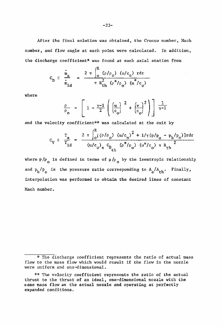
After the final solution was obtained, the Crocco number, Mach

number, and flow angle at each point were calculated. In addition,

the discharge coefficient* was found at each axial station from

where

m J..

[ 1 -1f ( (:J 2 + [:J 2

) J I y-l

and the velocity coefficient** was calculated at the exit by

R 2 2 ~ [(pIp) (u/c )+ l/y(p/p - Pb!po)]rdr o 0 0 0

where pIp is defined in terms of p Ip . by the isentropic relationship o 0

and Pb/Po is the pressure ratio corresponding to Ae/Ath. Finally,

interpolation was performed to obtain the desired lines of constant

Mach number.

* The discharge coefficient represents the ratio of actual mass flow to the mass flow which would result if the flow in the nozzle were uniform and one-dimensional.

** The velocity coefficient represents the ratio of the actual thrust to the thrust of an ideal, one-dimensional nozzle with the same mass flow as the actual nozzle and operating at perfectly expanded conditions.

4. RESULTS AND DISCUSSION

To determine the accuracy of the relaxation technique when applied

to the solution of transonic nozzle-flow problems, the procedure des­

cribed in the preceding section was coded for an IBM 370/158 digital

computer using FORTRAN IV (see Appendix for flow chart). The test case

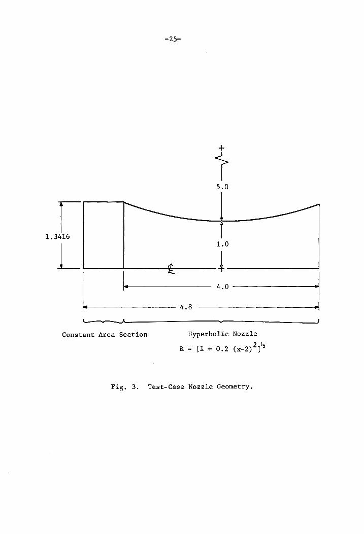
chosen was an axisymmetric, hyperbolic nozzle with a radius of curvature

of five inches and a throat radius of one inch (see Fig. 3). The

results of this calculation were compared with a theoretical solution

obtained by Hopkins and Hill (23) using a series expansion method. A

constant-area section upstream of the nozzle inlet was found necessary

to provide compatibility with the inlet boundary treatment which

was used.

The results presented here were obtained with a grid of 25 points

in the axial direction and 11 points in the radial direction. A solu­

tion was also obtained for a 25 x 21 grid, but these results differed

negligibly from the 25 x 11 grid and will therefore not be reported here.

The present solution is compared with the results of Hopkins and Hill

in Fig. 4, which shows lines of constant Mach number. The results

shown were obtained with 300 nozzle iterations. This was determined to

be the final solution by examination of the curves in Fig. 5 in which

the Mach number at various locations in the nozzle is plotted as a

function of the number of iterations. Inspection of this figure shows

that no significant change in the Mach number occurs after the 300th

iteration. The calculated points of constant Mach number in Fig. 4

-24-

-25-

+

t 5.0

r 1.3416

~ 1.0

------------------~

~------------------ 4.8

4.0~j

~ __ ----------------vv---------------__ ~ Constant Area Section

Fig. 3.

Hyperbolic Nozzle

R = [1 + 0.2 (x-2)2]~

Test-Case Nozzle Geometry.

1.2

1.0

,..... 0.8 .

f;: H ....... CI) 0.6 =' "r"I

"t:l ~ ~

0.4

0.2

0.0

-- Hopkins and Hill (23)

-1.5 -1.0 -0.5 o 0.5

Distance From Throat (In.)

Fig. 4. Lines of Constant Mach Number.

1.0 1.5

I N 0'\ I

+J or! ~ ~

::t:

+J ro 0 H

..c: E-i ~

+J Q)

'1"""1 ~

1-1 ::t:

2.20

2.10

2.00

1.90

1.80

1.12 .

1.08

1.04

1.00 .

0.96

0.40

0.30

0.20 .

0

-27-

100 200 300 400

Number of Iterations

Fig. 5. Change of Mach Number At Various Nozzle Locations With Number of Iterations (6 = Wall, 0 = Centerline).

500

-28-

show excellent agreement with the series expansion method in the

entire region shown.

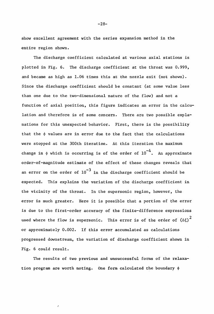
The discharge coefficient calculated at various axial stations is

plotted in Fig. 6. The discharge coefficient at the throat was 0.999,

and became as high as 1.06 times this at the nozzle exit (not shown).

Since the discharge coefficient should be constant (at some value less

than one due to the two-dimensional nature of the flow) and not a

function of axial position, this figure indicates an error in the calcu-

lation and therefore is of some concern. There are two possible expla­

nations for this unexpected behavior. First, there is the possibility

that the ~ values are in error due to the fact that the calculations

were stopped at the 300th iteration. At this iteration the maximum

change in ~ which is occurring is of the order of 10-4 • An approximate

order-of-magnitude estimate of the effect of these changes reveals that

an error on the order of 10-3 in the discharge coefficient should be

expected. This explains the variation of the discharge coefficient in

the vicinity of the throat. In the supersonic region, however, the

error is much greater. Here it is possible that a portion of the error

is due to the first-order accuracy of the finite-difference expressions

used where the flow is supersonic. This error is of the order of (~~)2

or approximately 0.002. If this error accumulated as calculations

progressed downstream, the variation of discharge coefficient shown in

Fig. 6 could result.

The results of two previous and unsuccessful forms of the relaxa­

tion program are worth noting. One form calculated the boundary ~

1.04

1.03

1.02

1.01

CD 1.00

0.99

0.98

0.97

-1.5 -1.0 -0.5 0 0.5

Distance From Throat (In.)

Fig. 6. Discharge Coefficient.

1.0 1.5

I N \.0 I

-30-

values at the wall and centerline from the radial first derivative of ~

at the adjacent~ interior points only, rather than by averaging the

derivatives as described in section 3.4. This effectively ignored the

known radial derivatives on the wall and centerline, and the results

shown in Fig. 7 underline the importance of imposing the proper boundary

conditions in obtaining an accurate solution. The second unsuccessful

program used type-dependent axial first derivatives in the column itera­

tion procedure, but calculated the axial first derivative by centered

differences everywhere for the final output after 300 iterations. These

results, shown in Fig. 7, are quite different from the output obtained

with type-dependent first derivatives (Fig. 4). The finite-difference

solution is thus dependent on the finite-difference expressions used in

its calculation, and these expressions cannot be changed even when

stability is no longer a factor.

Although successful runs were made with grids of 25 x 11 and 25 x

21 points, runs of a 49 x 21 grid failed because the column iterations

in the throat region did not converge. A slight improvement resulted

when centered differences were used to reassign the flow type in columns

which were indicated as being subsonic with backward differences. Also,

using under-relaxation in the column iterations themselves seemed to

improve convergence. A recent run which delayed the use of backward

differences until the physical throat was reached (instead of one or

two columns upstream of the throat) has allowed 25 complete nozzle

iterations with no apparent difficulties. At this time, all that can

be said is that the problem may be caused by the way in which the

1.2

1.0

--. . 0.8 ~

H '-"

CIl ::s 0.6 or!

"tj tU ~

0.4

0.2

0.0 -1.5

~ Supersonic Centered ¢~ ~ No ¢~ Averaging

Hopklns and Hill (23)

~ - \

~ 8J\ ~

~ ~

~ 11\, ~

Distance From Throat (In.)

& ~

....

Fig. 7. Effect of Boundary Treatment and Finite-Difference Form On Relaxation Solutions.

& I W ~ I

1.5

-32~

change of finite-difference expressions from centered to backward

is handled.

The CPU time required for 300 iterations of the 25 x 11 mesh was

199 seconds, corresponding to a time per point of 0.72 seconds. Normal­

izing this time with respect to an I~M 370/165 computer according to

Peitsch (24) gives a time per point of 0.24 seconds. This time is less

than that required by the time-dependent solutions of internal flow

tabulated by Brown (1) by an approximate factor of four and less than

the time required by error-minimization-type internal flow solutions by

a factor of five. Although this present method is not as fast as the

majority of external flow relaxation solutions, it must be kept in mind

that no attempt has been made to optimize the program logic from the

standpoint of computational efficiency. Variation of the subsonic

relaxation factor from 1.4 to 1.9 and the supersonic factor from 0.9

to 1.0 indicates that an optimum subsonic factor is given by Frankel's

method and that little improvement is obtained by an increase of the

supersonic factor. It is not unlikely, however, that refinements in

the program logic will produce significant improvements in the compu­

tational time.

5. CONCLUSIONS

The relaxation method reported here shows excellent agreement with

the series solution of Hopkins and Hill. In the throat region, the

calculated discharge coefficients are reasonable and within the expected

error. The computational time required is less than that of time­

dependent and error-minimization-type internal flow solutions. The

relaxation program in its present form is an accurate and competitive

computational tool for transonic nozzle-flow problems, and deserves

further development.

Further work is needed to devise a procedure for handling the

finite-difference scheme in the throat so that column convergence is

not jeopardized. Also program refinements should be sought to decrease

the computational time and thus further increase the computational­

speed advantage which the present method has over other nozzle analysis

methods.

-33-

6. APPENDIX

6.1 'DerivationOf~he'ColumnMatrixFormOf'The Governing Equation

The potential function form of Euler's equations is given in

Section 3.1 as

,,2 c r

J. = 0 (2) "'r •

When the transformation relations for the derivatives of ~ obtained

in Section 3.2 are introduced t the transformed governing equation can

be written as

222 2 (e - [~~ ~x + 4>~ ~x] ) (4)~~~x + ~~~~x~x + ~~~~x )

+ (e2

- [4>~~r]2) (4)~~~r2)

- 2(~~~x + ~~~x) (~~~r) (~~~~~~r + ~~~~x~r)

c2 + -

r

This equation is written in Section 3.2 as

where

A = ee2 - [~~~x + 4>~Wx]2) ~x2

B = (e2

- [4>~~x + ~~~x]2) ~x~x

- 2 (4)~~x + 4>~~x) (~w~r) ~x~r

C = (e2

- [4>~~x + ~~~x]2) ~x2

+ ee2 _ [$ ~ ]2) ~ 2 ~ r r

-34-

(3)

-35-

and

D = r

Because of its non-linear character, expressing this equation in

finite-difference form would result in an equation not suited to solution

by the Thomas algorithm. Thus the coefficients A, B, and C are taken to

be constants which are updated after each application of the Thomas

algorithm. Replacing the second derivatives in Eq. 3 by their finite-

difference approximations (for subsonic flow) gives

+ B($3 - $9 - $1 + $7)/(4d~6~)

+ C($2 - 2$5 + $8)/(6~)2 = D

where the nomenclature introduced in Fig. 2 has been used. Since it is

desired to solve the governing equation column by column and $2' $5'

and $8 all lie in the column under consideration, the equation above

is written as

C

(d1jJ) 2 $ -8

C = (d~)2

Similar consideration of a point lying in the supersonic region

of the flow field gives, in the nomenclature of Fig. 2,

-36-

A(~6 - 2~5 + ~4)/(~~)2

+ B ($3 - ~9 - ~l + ~7)(4~~6$)

+ c (<P3 - 2$6 + $9)/(6$)2 = D

or

[- B 46~6$ + (~:) 2 ] <P9 + [ (~;)2 2C ]

(6$)2 $6

+ [411~~ljJ + C ] ~ A (-2$5 + ~4) =

(~$) 2 3 (A~)2

Since it is assumed in the above equations that the central point

in the computational molecule lies in the interior region of the flow

field, consideration must next be given to points lying on the boundary

of the interior region (at j = 2 or J-l). At the nozzle wall ~2 or $3

(depending on whether the flow is subsonic or supersonic) is assumed

to be known, and at the nozzle centerline ~8 or <P9 is assumed to be

known. This means that the number of unknowns in the two'

equations written at the interior boundaries is reduced from three to

two. Therefore writing these equations for all interior points in a

given column gives rise to a set of simultaneous equations with a

tridiagonal coefficient matrix when written in the form

A 4> = f

of Section 3.2.

-37-

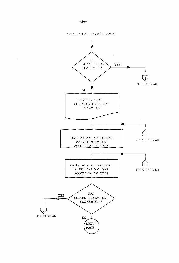
6.2 Flow Chart of RelaxatiortProgram

FROM PAGE 40

YES

-38-

START

INITIAL SOLUTION

BEGIN NOZZLE SCAN

CENTERED ~S AND ~~

BACKWARD ~S' CENTERED ~tjJ

CALCULATE q, , q, , AND M; x r

ASSIGN FLOW TYPE USING CENTERED DIFFERENCES

FROM PAGE 41

YES

2 TO PAGE 40

-39-

ENTER FROM PREVIOUS PAGE

NO

PRINT INITIAL SOLUTION ON FIRST

ITERATION

LOAD ARRAYS OF COLUMN MATRIX EQUATION

ACCORDING TO TYPE

CALCULATE ALL COLUMN FIRST DERIVATIVES ACCORDING TO TYPE

YES

TO PAGE 40

FROM PAGE 40

FROM PAGE 40

FROM PAGE 39

UPDATE COLUMN FIRST DERIVATIVES

TO PAGE 41

-40-

ENTER FROM PREVIOUS PAGE

NO

OBTAIN NEW COLUMN <pIS WITH TRI­

DIAGONAL ALGORITHM

OVER/UNDER- RELAX ENTIRE NOZZLE

CALCULATE M, a, CD' AND Cv

TO PAGE 39

3

TO PAGE 39

39

FROM PAGE 40

-41-

ENTER FROM PREVIOUS PAGE

PRINT PHI ARRAY, M, e, Cn' AND Cv

YES

STOP

TO' PAGE 38

NO

7 • REFERENCES

1. Brown, E. F., "Transonic Nozzle Flow: A Critical Survey of Analytical Methods," Douglas Aircraft Company, Report MDC J6223, September 1973.

2. Oswatitsch, K., and Rothstein, W., "Flow Pattern in a Converging -Diverging Nozzle," NACA Tech. Memo. No. 1215, 1949.

3. Barnwell, R. W., Theoretical Aerodynamics section, Loads Division, NASA Langley Research Center, Hampton, Va., Private Communication, January 1974.

4. Roache, P. J., Computational Fluid Dynamics, Hermosa Publishers, Albuquerque, N. M., 1972, pp. 114-117.

5. Murman, E. M., and Cole, J. D., "Calculation of Plane Steady Transonic Flows," AIM J., Vol. 9, No.1, January 1971, pp. l14'!"" 121.

6. Murman, E. M., "Computational Methods for Inviscid Transonic Flows With Imbedded Shock Waves," Numerical 'Methods 'in Fluid Dynamics, J. J. Smolderen, Ed., AGARD Lecture Series No. 48, May 1972, pp. 13/1 - 13/34.

7. Carnahan, B., Luther, H. A., and Wilkes, J. 0., Applied Numerical Methods, John Wiley & Sons, Inc., New York, 1969, pp. 441-446.

8. Murman, E. M., and Krupp, J. A., "Solution of the Transonic Potential Equation Using a Mixed Finite Difference System" Proceedirtgsof the Second International Conference on Numerical Methods in Fluid Dynamics, M. Holt, Ed., Lecture Notes in Physics, Vol. 8, Springer­Verlag, 1970, pp. 199-208.

9. Krupp, J. A., and Murman, E. M., "The Numerical Calculation of Steady Transonic Flows Past Thin Lifting Airfoils and Slender Bodies," AIM Paper No. 71-566, 1971.

10. Bailey, F. R., "Numerical Calculation of Transonic Flow About Slender Bodies of Revolution," NASA TN D-6582, December 1971.

11. Bailey, F. R., and Ballhaus, t~. F., "Relaxation Methods for Transonic Flow About Wing-Cylinder Combinations and Lifting Swept Wings," Proceedings of The 'Third Intetnational'Conference on Numerical Methods in Fluid Mechanics, Vol. II, July 3-7, 1972, H. Cabannes and R. Temam, Eds., Lecture Notes in Physics, Vol. 19, Springer-Verlag, 1973.

12. Ballhaus, W. F., and Bailey, F. R., "Numerical Calculation of Transonic Flow About Swept Wings," AlAA Paper No. 72-677, 1972.

-42-

-43-

13. Caughey, D. A., "A New Transonic Small Disturbance Theory for Numerical Analysis," McDonnell Douglas Research Laboratories, Report MOC Q0478, December 1972.

14. Bailey, F. R., and Steger, J. L., "Relaxati.on Techniques for Three­Dimensional Transonic Flow About Wings," AIM Paper No. 72-189, 1972.

15. Yoshihara, H., "Computational Methods for 2D and 3D Transonic Flows with Shocks," General Dynamics, Report No. GDCA-ERR-l726, December 1972.

16. Krupp, J., "The Numerical Calculation of Plane Steady Transonic Flows Past Thin Lifting Airfoils," Boeing Co. Report D180-23958-l, 1971.

17. Garabedian, P., and Korn, D., "Analysis of Transonic Airfoils," Comma Pur~pl. Math., Vol. XXIV, 1971, pp. 841-851.

18. Steger, J. L., and Lomax, H., "Generalized Relaxation Methods Applied to Problems in Transonic Flow,tf Proceedings of the Second International Conference on Numerical Methods in Fluid Dynamics, M. Holt, Ed., Lecture Notes in Physics, Vol. 8, Springer-Verlag, 1970, pp. 193-197.

19. Colehour, J. L., "Transonic Flow Analysis Using a Streamline Coordinate Transformation Procedure,H AIM Paper No. 73-657, 1973.

20. Jameson, A., "Numerical Calculation of the Three Dimensional Tran­sonic Flow Over a Yawed Wing," Proceedings AIM Computational Fluid Dynamics Conference, Palm Springs, California, July 19-20, 1973, pp. 18-26.

21. South, J. C., Jr., and Jameson, A., "Rela.xation Solutions for Inviscid Axisymmetric Transonic Flow Over Blunt or Pointed Bodies," Proceedings AIM Computational Fluid Dynamics Conference, Palm Springs, California, July 19-20, 1973, pp. 8-17.

22. Steger, J. L., and Lomax, H., "Numerical Calculation of Transonic Flow About Two-Dimensional Airfoils by Relaxation Procedures," AIM Paper No. 71-569, 1971.

23. Hopkins, D. F., and Hill, D. E., f1Effect of Small Radius of Curvature on Transonic Flow in Axisymmetric Nozzles," AIM J., Vol. 4, No.8, August 1966, pp. 1337-1343.

24. Peitsch, H. E., Manager, Technical Services Development, McDonnell Douglas Automation Co., Huntington Beach, California, Private Communication, August 1974.

8. VITA

The author was born on July 10, 1950, in Alexandria, Virginia. He

attended school in Annandale, Virginia; Djakarta, Indonesia; and Manila,

Republic of the Philippines. He graduated from Annandale High School in

June of 1968.

In September of 1968 he entered Virginia Polytechnic Institute and

State University_ While there he participated in the Cooperative

Education Program, working for the Ford Motor Company and the Central

Intelligence Agency_ He obtained a Bachelor of Science degree in

Mechanical Engineering in June of 1973, and began graduate study in

September of that year toward a Master of Science degree in Mechanical

Engineering.

The author is a member of Pi Tau Sigma and the American Society of

Mechanical Engineers, and is an Engineer-in-Training registered with

the Commonwealth of Virginia. He is presently employed as a product

engineer at the Allegany Ballistics Laboratory of Hercules, Inc.

-44-

AN ~~LICATION OF RELAXATION METHODS

TO

TRANSONIC NOZZLE FLOW

By

Kevin Eugene Walsh

(ABSTRACT)

An application of relaxation techniques to the solution of transonic

flow in a converging - diverging nozzle is presented. The assumptions

of steady, isentropic flow of a perfect gas were made. Successive line

relaxation, similar to that of Garabedian and Korn, was employed in a

transformed computational plane. The potential function at interior

points was obtained column by column through repeated application of the

Thomas algorithm. Once the interior-point calculations were complete

the values of the potential function on the boundaries were obtained by

extrapolation using the wall-tangency and centerline-symmetry conditions

where appropriate. A final solution was considered obtained when negli­

gible changes were observed in the Mach number at all flow-field points

from one iteration to the next.

To determine the accuracy of the method, the flow through a hyper­

bolic converging - diverging nozzle was calculated and the results were

compared with an existing solution obtained by a series expansion method.

The calculated lines of constant Mach number were in excellent agreement

with the series expansion solution. The time required for this solution

was faster than time-dependent and error-minimization-type solutions

by more than a factor of four even though no attempt was made to opti­

mize the computational efficiency of the program logic.