IEEE ROBOTICS AND AUTOMATION LETTERS. PREPRINT VERSION. ACCEPTED JANUARY, 2017 1

An Approach for Imitation Learning on Riemannian Manifolds

Martijn J.A. Zeestraten1, Ioannis Havoutis2,3, Joao Silverio1, Sylvain Calinon2,1, Darwin. G. Caldwell1

Abstract—In imitation learning, multivariate Gaussians arewidely used to encode robot behaviors. Such approaches do notprovide the ability to properly represent end-effector orientation,as the distance metric in the space of orientations is notEuclidean. In this work we present an extension of commonimitation learning techniques to Riemannian manifolds. Thisgeneralization enables the encoding of joint distributions thatinclude the robot pose. We show that Gaussian conditioning,Gaussian product and nonlinear regression can be achievedwith this representation. The proposed approach is illustratedwith examples on a 2-dimensional sphere, with an example ofregression between two robot end-effector poses, as well as anextension of Task-Parameterized Gaussian Mixture Model (TP-GMM) and Gaussian Mixture Regression (GMR) to Riemannianmanifolds.

Index Terms—Learning and Adaptive Systems, Probability andStatistical Methods

I. INTRODUCTION

THE Gaussian is the most common distribution for the

analysis of continuous data streams. Its popularity can

be explained on both theoretical and practical grounds. The

Gaussian is the maximum entropy distribution for data defined

in Euclidean spaces: it makes the least amount of assumptions

about the distribution of a dataset given its first two moments

[1]. In addition, operations such as marginalization, condition-

ing, linear transformation and multiplication, all result in a

Gaussian.

In imitation learning, multivariate Gaussians are widely used

to encode robot motion [2]. Generally, one encodes a joint

distribution over the motion variables (e.g. time and pose),

and uses statistical inference to estimate an output variable

(e.g. desired pose) given an input variable (e.g. time). The

variance and correlation encoded in the Gaussian allow for

interpolation and, to some extent, extrapolation of the original

demonstration data. Regression with a mixture of Gaussians

is fast compared to data-driven approaches, because it does

not depend on the original training data. Multiple models

relying on Gaussian properties have been proposed, including

Manuscript received: September, 10, 2016; Revised December, 8, 2016;Accepted January, 3, 2017.

This paper was recommended for publication by Editor Dongheui Lee uponevaluation of the Associate Editor and Reviewers’ comments. The researchleading to these results has received funding from the People Programme(Marie Curie Actions) of the European Union’s 7th Framework ProgrammeFP7/2007-2013/ under REA grant agreement number 608022. It is alsosupported by the DexROV Project through the EC Horizon 2020 programme(Grant #635491) and by the Swiss National Science Foundation through theI-DRESS project (CHIST-ERA).

1 Department of Advanced Robotics, Istituto Italiano di Tecnologia, ViaMorego 30, 16163 Genova, Italy. name.surname@iit.it

2 Idiap Research Institute, Rue Marconi 19, 1920 Martigny, Switzerland.name.surname@idiap.ch

3 Oxford Robotics Institute, Department of Engineering Science, Universityof Oxford, United Kingdom. ihavoutis@robots.ox.ac.uk

Digital Object Identifier (DOI): see top of this page.

distributions over movement trajectories [3], and the encoding

of movement from multiple perspectives [4].

Probabilistic encoding using Gaussians is restricted to vari-

ables that are defined in the Euclidean space. This typically

excludes the use of end-effector orientation. Although one can

approximate orientation locally in the Euclidean space [5], this

approach becomes inaccurate when there is large variance in

the orientation data.

The most compact and complete representation for orienta-

tion is the unit quaternion1. Quaternions can be represented

as elements of the 3-sphere, a 3 dimensional Riemannian

manifold. Riemannian manifolds allow various notions such as

length, angles, areas, curvature or divergence to be computed,

which is convenient in many applications including statistics,

optimization and metric learning [6]–[9].

In this work we present a generalization of common prob-

abilistic imitation learning techniques to Riemannian mani-

folds. Our contributions are twofold: (i) We show how to

derive Gaussian conditioning and Gaussian product through

likelihood maximization. The derivation demonstrates that

parallel transportation of the covariance matrices is essential

for Gaussian conditioning and Gaussian product. This aspect

was not considered in previous generalizations of Gaussian

conditioning to Riemannian manifolds [10], [11]; (ii) We show

how the elementary operations of Gaussian conditioning and

Gaussian product can be used to extend Task-Parameterized

Gaussian Mixture Model (TP-GMM) and Gaussian Mixture

Regression (GMR) to Riemannian manifolds.

This paper is organized as follows: Section II introduces

Riemannian manifolds and statistics. The proposed methods

are detailed in Section III, evaluated in Section IV, and

discussed in relation to previous work in Section V. Section

VI concludes the paper. This paper is accompanied by a video.

Source code related to the work presented is available through

http://www.idiap.ch/software/pbdlib/.

II. PRELIMINARIES

Our objective is to extend common methods for imitation

learning from Euclidean space to Riemannian manifolds. Un-

like the Euclidean space, the Riemannian Manifold is not a

vector space where sum and scalar multiplication are defined.

Therefore, we cannot directly apply Euclidean methods to data

defined on a Riemannian manifold. However, these methods

can be applied in the Euclidean tangent spaces of the manifold,

which provide a way to indirectly perform computation on the

manifold. In this section we introduce the notions required to

enable such indirect computations to generalize methods for

imitation learning to Riemannian manifolds. We first introduce

1A unit quaternion is a quaternion with unit norm. From here on, we willjust use quaternion to refer to the unit quaternion.

2 IEEE ROBOTICS AND AUTOMATION LETTERS. PREPRINT VERSION. ACCEPTED JANUARY, 2017

=Logg(p)

p=Expg( )

g

TgM

(a)

gpg

phh

Ahg (pg)

(b)

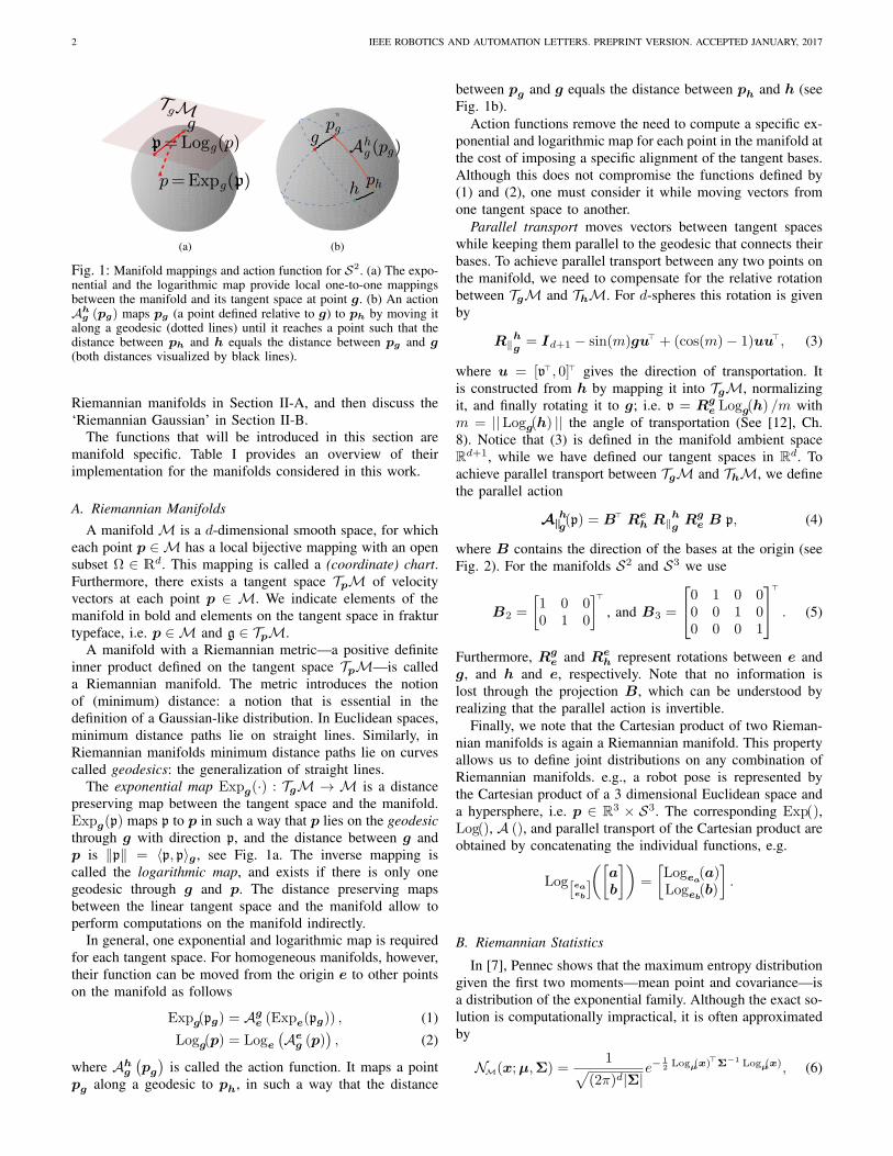
Fig. 1: Manifold mappings and action function for S2. (a) The expo-nential and the logarithmic map provide local one-to-one mappingsbetween the manifold and its tangent space at point g. (b) An actionAh

g (pg) maps pg (a point defined relative to g) to ph by moving italong a geodesic (dotted lines) until it reaches a point such that thedistance between ph and h equals the distance between pg and g(both distances visualized by black lines).

Riemannian manifolds in Section II-A, and then discuss the

‘Riemannian Gaussian’ in Section II-B.

The functions that will be introduced in this section are

manifold specific. Table I provides an overview of their

implementation for the manifolds considered in this work.

A. Riemannian Manifolds

A manifoldM is a d-dimensional smooth space, for which

each point p ∈M has a local bijective mapping with an open

subset Ω ∈ Rd. This mapping is called a (coordinate) chart.

Furthermore, there exists a tangent space TpM of velocity

vectors at each point p ∈ M. We indicate elements of the

manifold in bold and elements on the tangent space in fraktur

typeface, i.e. p ∈M and g ∈ TpM.

A manifold with a Riemannian metric—a positive definite

inner product defined on the tangent space TpM—is called

a Riemannian manifold. The metric introduces the notion

of (minimum) distance: a notion that is essential in the

definition of a Gaussian-like distribution. In Euclidean spaces,

minimum distance paths lie on straight lines. Similarly, in

Riemannian manifolds minimum distance paths lie on curves

called geodesics: the generalization of straight lines.

The exponential map Expg(·) : TgM → M is a distance

preserving map between the tangent space and the manifold.

Expg(p) maps p to p in such a way that p lies on the geodesic

through g with direction p, and the distance between g and

p is ‖p‖ = 〈p, p〉g , see Fig. 1a. The inverse mapping is

called the logarithmic map, and exists if there is only one

geodesic through g and p. The distance preserving maps

between the linear tangent space and the manifold allow to

perform computations on the manifold indirectly.

In general, one exponential and logarithmic map is required

for each tangent space. For homogeneous manifolds, however,

their function can be moved from the origin e to other points

on the manifold as follows

Expg(pg) = Age (Expe(pg)) , (1)

Logg(p) = Loge(

Aeg (p)

)

, (2)

where Ahg

(

pg

)

is called the action function. It maps a point

pg along a geodesic to ph, in such a way that the distance

between pg and g equals the distance between ph and h (see

Fig. 1b).

Action functions remove the need to compute a specific ex-

ponential and logarithmic map for each point in the manifold at

the cost of imposing a specific alignment of the tangent bases.

Although this does not compromise the functions defined by

(1) and (2), one must consider it while moving vectors from

one tangent space to another.

Parallel transport moves vectors between tangent spaces

while keeping them parallel to the geodesic that connects their

bases. To achieve parallel transport between any two points on

the manifold, we need to compensate for the relative rotation

between TgM and ThM. For d-spheres this rotation is given

by

R‖h

g= Id+1 − sin(m)gu⊤ + (cos(m)− 1)uu⊤, (3)

where u = [v⊤, 0]⊤ gives the direction of transportation. It

is constructed from h by mapping it into TgM, normalizing

it, and finally rotating it to g; i.e. v = Rge Logg(h) /m with

m = ||Logg(h) || the angle of transportation (See [12], Ch.

8). Notice that (3) is defined in the manifold ambient space

Rd+1, while we have defined our tangent spaces in R

d. To

achieve parallel transport between TgM and ThM, we define

the parallel action

A‖h

g(p) = B⊤ Re

h R‖h

gRg

e B p, (4)

where B contains the direction of the bases at the origin (see

Fig. 2). For the manifolds S2 and S3 we use

B2 =

[

1 0 00 1 0

]

⊤

, and B3 =

0 1 0 00 0 1 00 0 0 1

⊤

. (5)

Furthermore, Rge and Re

h represent rotations between e and

g, and h and e, respectively. Note that no information is

lost through the projection B, which can be understood by

realizing that the parallel action is invertible.

Finally, we note that the Cartesian product of two Rieman-

nian manifolds is again a Riemannian manifold. This property

allows us to define joint distributions on any combination of

Riemannian manifolds. e.g., a robot pose is represented by

the Cartesian product of a 3 dimensional Euclidean space and

a hypersphere, i.e. p ∈ R3 × S3. The corresponding Exp(),

Log(), A (), and parallel transport of the Cartesian product are

obtained by concatenating the individual functions, e.g.

Log[eaeb

]

([

a

b

])

=

[

Logea(a)

Logeb(b)

]

.

B. Riemannian Statistics

In [7], Pennec shows that the maximum entropy distribution

given the first two moments—mean point and covariance—is

a distribution of the exponential family. Although the exact so-

lution is computationally impractical, it is often approximated

by

NM(x;µ,Σ) =1

√

(2π)d|Σ|e−

1

2Logµ(x)

⊤Σ

−1 Logµ(x), (6)

ZEESTRATEN et al.: AN APPROACH FOR IMITATION LEARNING ON RIEMANNIAN MANIFOLDS 3

e

(a)

TgM

g

h= g

h=Ahg ( g)

Th M

g

e

h

(b)

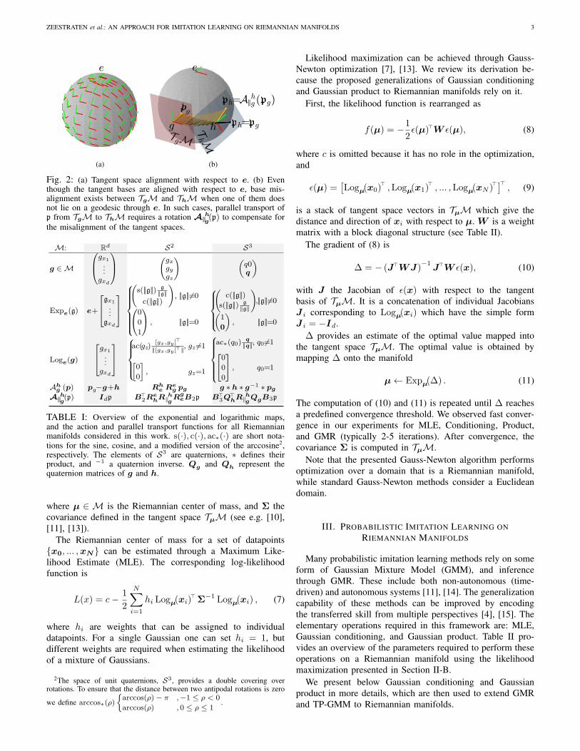
Fig. 2: (a) Tangent space alignment with respect to e. (b) Eventhough the tangent bases are aligned with respect to e, base mis-alignment exists between TgM and ThM when one of them doesnot lie on a geodesic through e. In such cases, parallel transport ofp from TgM to ThM requires a rotation A‖

h

g(p) to compensate for

the misalignment of the tangent spaces.

M: Rd S2 S3

g ∈ M

gx1

...gxd

(

gxgygz

)

(

q0q

)

Expe(g) e+

gx1

...gxd

(

s(||g||) g

||g||

c(||g||)

)

, ||g||6=0

0

0

1

, ||g||=0

(

c(||g||)

s(||g||) g

||g||

)

,||g||6=0

(

1

0

)

, ||g||=0

Loge(g)

gx1

...gxd

ac(gz)[gx,gy ]

⊤

||[gx,gy ]⊤||, gz 6=1

[

0

0

]

, gz=1

ac∗(q0)q

||q||, q0 6=1

0

0

0

, q0=1

Ahg (p) pg−g+h Rh

e Reg pg g ∗ h ∗ g−1 ∗ pg

A‖hg(p) Idp B⊤

2RehR‖

hgR

geB2p B⊤

3Q⊤

hR‖hgQgB3p

TABLE I: Overview of the exponential and logarithmic maps,and the action and parallel transport functions for all Riemannianmanifolds considered in this work. s(·), c(·), ac∗(·) are short nota-tions for the sine, cosine, and a modified version of the arccosine2,respectively. The elements of S3 are quaternions, ∗ defines theirproduct, and −1 a quaternion inverse. Qg and Qh represent thequaternion matrices of g and h.

where µ ∈ M is the Riemannian center of mass, and Σ the

covariance defined in the tangent space TµM (see e.g. [10],

[11], [13]).

The Riemannian center of mass for a set of datapoints

x0, ... ,xN can be estimated through a Maximum Like-

lihood Estimate (MLE). The corresponding log-likelihood

function is

L(x) = c−1

2

N∑

i=1

hi Logµ(xi)⊤

Σ−1 Logµ(xi) , (7)

where hi are weights that can be assigned to individual

datapoints. For a single Gaussian one can set hi = 1, but

different weights are required when estimating the likelihood

of a mixture of Gaussians.

2The space of unit quaternions, S3, provides a double covering overrotations. To ensure that the distance between two antipodal rotations is zero

we define arccos∗(ρ)

arccos(ρ)− π ,−1 ≤ ρ < 0

arccos(ρ) , 0 ≤ ρ ≤ 1.

Likelihood maximization can be achieved through Gauss-

Newton optimization [7], [13]. We review its derivation be-

cause the proposed generalizations of Gaussian conditioning

and Gaussian product to Riemannian manifolds rely on it.

First, the likelihood function is rearranged as

f(µ) = −1

2ǫ(µ)⊤W ǫ(µ), (8)

where c is omitted because it has no role in the optimization,

and

ǫ(µ) =[

Logµ(x0)⊤

,Logµ(x1)⊤

, ... ,Logµ(xN )⊤]

⊤

, (9)

is a stack of tangent space vectors in TµM which give the

distance and direction of xi with respect to µ. W is a weight

matrix with a block diagonal structure (see Table II).

The gradient of (8) is

∆ = − (J⊤WJ)−1

J⊤W ǫ(x), (10)

with J the Jacobian of ǫ(x) with respect to the tangent

basis of TµM. It is a concatenation of individual Jacobians

J i corresponding to Logµ(xi) which have the simple form

J i = −Id.

∆ provides an estimate of the optimal value mapped into

the tangent space TµM. The optimal value is obtained by

mapping ∆ onto the manifold

µ← Expµ(∆) . (11)

The computation of (10) and (11) is repeated until ∆ reaches

a predefined convergence threshold. We observed fast conver-

gence in our experiments for MLE, Conditioning, Product,

and GMR (typically 2-5 iterations). After convergence, the

covariance Σ is computed in TµM.

Note that the presented Gauss-Newton algorithm performs

optimization over a domain that is a Riemannian manifold,

while standard Gauss-Newton methods consider a Euclidean

domain.

III. PROBABILISTIC IMITATION LEARNING ON

RIEMANNIAN MANIFOLDS

Many probabilistic imitation learning methods rely on some

form of Gaussian Mixture Model (GMM), and inference

through GMR. These include both non-autonomous (time-

driven) and autonomous systems [11], [14]. The generalization

capability of these methods can be improved by encoding

the transferred skill from multiple perspectives [4], [15]. The

elementary operations required in this framework are: MLE,

Gaussian conditioning, and Gaussian product. Table II pro-

vides an overview of the parameters required to perform these

operations on a Riemannian manifold using the likelihood

maximization presented in Section II-B.

We present below Gaussian conditioning and Gaussian

product in more details, which are then used to extend GMR

and TP-GMM to Riemannian manifolds.

4 IEEE ROBOTICS AND AUTOMATION LETTERS. PREPRINT VERSION. ACCEPTED JANUARY, 2017

ǫ(µ) W J ∆ Σ

ML

E

Logµ(xn)...

Logµ(xn)

diag

Σ−1

...

Σ−1

−I...

−I

1∑

Ni

hi

N∑

n=1hi Logµ(xn)

1∑

Ni

hi

N∑

n=1hi Logµ(xn) Logµ(xn)

⊤

Pro

du

ct

−Logµ(µ1)...

−Logµ(µP )

diag

Σ−1‖1...

Σ−1‖P

−I...

−I

(

P∑

p=1Σ

−1

‖p

)−1P∑

p=1Σ

−1‖p

Logµ(

µp

)

(

∑Pp=1 Σ

−1‖p

)−1

Co

nd

itio

n

[

LogxI(µI)

LogxO(µO)

]

Λ‖

[

0

−I

]

LogxO(µO) +Λ

−1‖OO

Λ⊤

‖OILogxI(µI

) Λ−1‖OO

TABLE II: Overview of the parameters used in the likelihood maximization procedure presented in Sections II-B, III-A and

III-B.

g1

g2

g1g2

(a)

g1

g2

g1g2

(b)

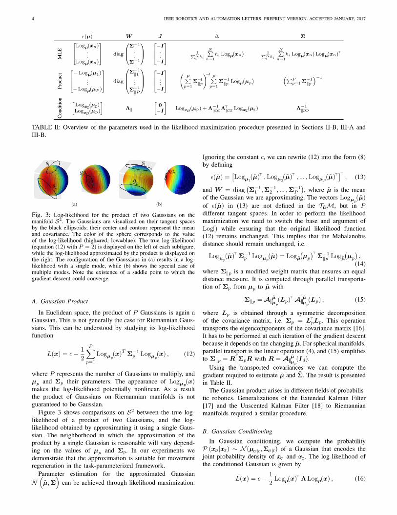
Fig. 3: Log-likelihood for the product of two Gaussians on themanifold S2. The Gaussians are visualized on their tangent spacesby the black ellipsoids; their center and contour represent the meanand covariance. The color of the sphere corresponds to the valueof the log-likelihood (high=red, low=blue). The true log-likelihood(equation (12) with P = 2) is displayed on the left of each subfigure,while the log-likelihood approximated by the product is displayed onthe right. The configuration of the Gaussians in (a) results in a log-likelihood with a single mode, while (b) shows the special case ofmultiple modes. Note the existence of a saddle point to which thegradient descent could converge.

A. Gaussian Product

In Euclidean space, the product of P Gaussians is again a

Gaussian. This is not generally the case for Riemannian Gaus-

sians. This can be understood by studying its log-likelihood

function

L(x) = c−1

2

P∑

p=1

Logµp(x)

TΣ

−1p Logµp

(x) , (12)

where P represents the number of Gaussians to multiply, and

µp and Σp their parameters. The appearance of Logµp(x)

makes the log-likelihood potentially nonlinear. As a result

the product of Gaussians on Riemannian manifolds is not

guaranteed to be Gaussian.

Figure 3 shows comparisons on S2 between the true log-

likelihood of a product of two Gaussians, and the log-

likelihood obtained by approximating it using a single Gaus-

sian. The neighborhood in which the approximation of the

product by a single Gaussian is reasonable will vary depend-

ing on the values of µp and Σp. In our experiments we

demonstrate that the approximation is suitable for movement

regeneration in the task-parameterized framework.

Parameter estimation for the approximated Gaussian

N(

µ, Σ)

can be achieved through likelihood maximization.

Ignoring the constant c, we can rewrite (12) into the form (8)

by defining

ǫ(µ) =[

Logµ1

(µ)⊤

,Logµ2

(µ)⊤

, ... ,LogµP(µ)

⊤]⊤

, (13)

and W = diag(

Σ−11 ,Σ−1

2 , ... ,Σ−1P

)

, where µ is the mean

of the Gaussian we are approximating. The vectors Logµp(µ)

of ǫ(µ) in (13) are not defined in the TµM, but in Pdifferent tangent spaces. In order to perform the likelihood

maximization we need to switch the base and argument of

Log() while ensuring that the original likelihood function

(12) remains unchanged. This implies that the Mahalanobis

distance should remain unchanged, i.e.

Logµp(µ)

⊤

Σ−1p Logµp

(µ) = Logµ(

µp

)

⊤

Σ−1‖p Logµ

(

µp

)

,(14)

where Σ‖p is a modified weight matrix that ensures an equal

distance measure. It is computed through parallel transporta-

tion of Σp from µp to µ with

Σ‖p = A‖µ

µp

(Lp)⊤

A‖µ

µp

(Lp) , (15)

where Lp is obtained through a symmetric decomposition

of the covariance matrix, i.e. Σp = L⊤

pLp. This operation

transports the eigencomponents of the covariance matrix [16].

It has to be performed at each iteration of the gradient descent

because it depends on the changing µ. For spherical manifolds,

parallel transport is the linear operation (4), and (15) simplifies

to Σ‖p = R⊤ΣpR with R = A‖

µ

µp

(Id).

Using the transported covariances we can compute the

gradient required to estimate µ and Σ. The result is presented

in Table II.

The Gaussian product arises in different fields of probabilis-

tic robotics. Generalizations of the Extended Kalman Filter

[17] and the Unscented Kalman Filter [18] to Riemannian

manifolds required a similar procedure.

B. Gaussian Conditioning

In Gaussian conditioning, we compute the probability

P (xO|xI) ∼ N (µO|I,ΣO|I) of a Gaussian that encodes the

joint probability density of xO and xI . The log-likelihood of

the conditioned Gaussian is given by

L(x) = c−1

2Logµ(x)

⊤

ΛLogµ(x) , (16)

ZEESTRATEN et al.: AN APPROACH FOR IMITATION LEARNING ON RIEMANNIAN MANIFOLDS 5

with

x =

[

xI

xO

]

, µ =

[

µI

µO

]

, Λ =

[

ΛII ΛIO

ΛOI ΛOO

]

, (17)

where the subscriptsO andI indicate respectively the input and

the output, and the precision matrix Λ = Σ−1 is introduced

to simplify the derivation.

Equation (16) is in the form of (8). Here we want to estimate

xO given xI (i.e. µO|I). Similarly to the Gaussian product, we

cannot directly optimize (16) because the dependent variable,

xO, is in the argument of the logarithmic map. This is again

resolved by parallel transport, namely

Λ‖ = A‖x

µ(V )

⊤

A‖x

µ(V ) , (18)

where V is obtained through a symmetric decomposition of

the precision matrix: Λ = V⊤V . Using the transformed

precision matrix, the values for ǫ(xt), and J (both found in

Table II), we can apply (11) to obtain the update rule. The

covariance obtained through Gaussian conditioning is given by

Λ−1‖ . Note that we maximize the likelihood only with respect

to xO, and therefore 0 appears in the Jacobian.

C. Gaussian Mixture Regression

Similarly to a Gaussian Mixture Model (GMM) in Eu-

clidean space, a GMM on a Riemannian manifold is defined

by a weighted sum of Gaussians

P (x) =

K∑

i=1

πiN (x;µi,Σi),

where πi are the priors, with∑K

i πi = 1. In imitation

learning, they are used to represent nonlinear behaviors in a

probabilistic manner. Parameters of the GMM can be estimated

by Expectation Maximization (EM), an iterative process in

which the data are given weights for each cluster (Expectation

step), and in which the clusters are subsequently updated using

a weighted MLE (Maximization step). We refer to [10] for a

detailed description of EM for Riemannian GMMs.

A popular regression technique for Euclidean GMM is

Gaussian Mixture Regression (GMR) [4]. It approximates the

conditioned GMM using a single Gaussian, i.e.

P (xO|xI) ≈ N(

µO, ΣO

)

.

In Euclidean space, the parameters of this Gaussian are formed

by a weighted sum of the expectations and covariances,

namely,

µO=

K∑

i=1

hi E [N (xO|xI;µi,Σi)] , (19)

ΣO =

K∑

i=1

hi cov[N (xO|xI;µi,Σi)] , (20)

with hi =N

(

xI;µi,I,Σi,II

)

∑K

j=1N(

xI;µj,I,Σj,II

). (21)

We cannot directly apply (19) and (20) to a GMM defined

on a Riemannian manifold. First, because the computation of

A

e

(a) Transformation A (b) Translation b

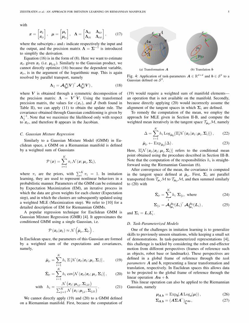
Fig. 4: Application of task-parameters A ∈ Rd×d and b ∈ S2 to a

Gaussian defined on S2.

(19) would require a weighted sum of manifold elements—

an operation that is not available on the manifold. Secondly,

because directly applying (20) would incorrectly assume the

alignment of the tangent spaces in which Σi are defined.

To remedy the computation of the mean, we employ the

approach for MLE given in Section II-B, and compute the

weighted mean iteratively in the tangent space TµOM, namely

∆ =

K∑

i=1

hi LogµO(E[N (xO|xI;µi,Σi)]) , (22)

µO← ExpµO

(∆) . (23)

Here, E[N (xO|xI;µi,Σi)] refers to the conditional mean

point obtained using the procedure described in Section III-B.

Note that the computation of the responsibilities hi is straight-

forward using the Riemannian Gaussian (6).

After convergence of the mean, the covariance is computed

in the tangent space defined at µO

. First, Σi are parallel

transported from TµiM to TµO

M, and then summed similarly

to (20) with

ΣO =

K∑

i

hi Σ‖i, where (24)

Σ‖i = A‖µO

µi

(Li)⊤

A‖µO

µi

(Li) , (25)

and Σi = LiL⊤

i .

D. Task-Parameterized Models

One of the challenges in imitation learning is to generalize

skills to previously unseen situations, while keeping a small set

of demonstrations. In task-parameterized representations [4],

this challenge is tackled by considering the robot end-effector

motion from different perspectives (frames of reference such

as objects, robot base or landmarks). These perspectives are

defined in a global frame of reference through the task

parameters A and b, representing a linear transformation and

translation, respectively. In Euclidean spaces this allows data

to be projected to the global frame of reference through the

linear operation Au+ b.

This linear operation can also be applied to the Riemannian

Gaussian, namely

µA,b = Expb(ALoge(µ)) , (26)

ΣA,b = (AΣA⊤)‖µA,b

b

, (27)

6 IEEE ROBOTICS AND AUTOMATION LETTERS. PREPRINT VERSION. ACCEPTED JANUARY, 2017

1

2

3

e

1

2

3

e

(a)

12

31

2

3

e

e2

e1

(b)

e1

e2

e

(c)

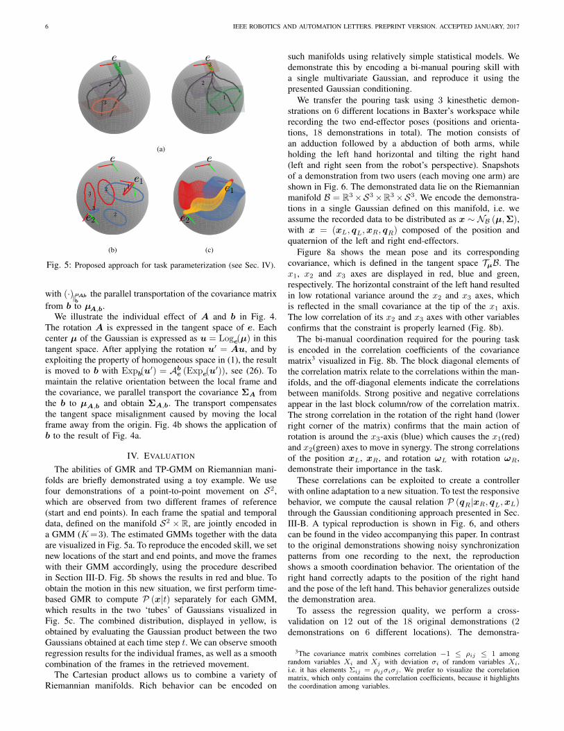
Fig. 5: Proposed approach for task parameterization (see Sec. IV).

with (·)‖µA,b

b

the parallel transportation of the covariance matrix

from b to µA,b.

We illustrate the individual effect of A and b in Fig. 4.

The rotation A is expressed in the tangent space of e. Each

center µ of the Gaussian is expressed as u = Loge(µ) in this

tangent space. After applying the rotation u′ = Au, and by

exploiting the property of homogeneous space in (1), the result

is moved to b with Expb(u′) = Ab

e (Expe(u′)), see (26). To

maintain the relative orientation between the local frame and

the covariance, we parallel transport the covariance ΣA from

the b to µA,b and obtain ΣA,b. The transport compensates

the tangent space misalignment caused by moving the local

frame away from the origin. Fig. 4b shows the application of

b to the result of Fig. 4a.

IV. EVALUATION

The abilities of GMR and TP-GMM on Riemannian mani-

folds are briefly demonstrated using a toy example. We use

four demonstrations of a point-to-point movement on S2,

which are observed from two different frames of reference

(start and end points). In each frame the spatial and temporal

data, defined on the manifold S2 × R, are jointly encoded in

a GMM (K=3). The estimated GMMs together with the data

are visualized in Fig. 5a. To reproduce the encoded skill, we set

new locations of the start and end points, and move the frames

with their GMM accordingly, using the procedure described

in Section III-D. Fig. 5b shows the results in red and blue. To

obtain the motion in this new situation, we first perform time-

based GMR to compute P (x|t) separately for each GMM,

which results in the two ‘tubes’ of Gaussians visualized in

Fig. 5c. The combined distribution, displayed in yellow, is

obtained by evaluating the Gaussian product between the two

Gaussians obtained at each time step t. We can observe smooth

regression results for the individual frames, as well as a smooth

combination of the frames in the retrieved movement.

The Cartesian product allows us to combine a variety of

Riemannian manifolds. Rich behavior can be encoded on

such manifolds using relatively simple statistical models. We

demonstrate this by encoding a bi-manual pouring skill with

a single multivariate Gaussian, and reproduce it using the

presented Gaussian conditioning.

We transfer the pouring task using 3 kinesthetic demon-

strations on 6 different locations in Baxter’s workspace while

recording the two end-effector poses (positions and orienta-

tions, 18 demonstrations in total). The motion consists of

an adduction followed by a abduction of both arms, while

holding the left hand horizontal and tilting the right hand

(left and right seen from the robot’s perspective). Snapshots

of a demonstration from two users (each moving one arm) are

shown in Fig. 6. The demonstrated data lie on the Riemannian

manifold B = R3×S3×R

3×S3. We encode the demonstra-

tions in a single Gaussian defined on this manifold, i.e. we

assume the recorded data to be distributed as x ∼ NB (µ,Σ),with x = (xL, qL,xR, qR) composed of the position and

quaternion of the left and right end-effectors.

Figure 8a shows the mean pose and its corresponding

covariance, which is defined in the tangent space TµB. The

x1, x2 and x3 axes are displayed in red, blue and green,

respectively. The horizontal constraint of the left hand resulted

in low rotational variance around the x2 and x3 axes, which

is reflected in the small covariance at the tip of the x1 axis.

The low correlation of its x2 and x3 axes with other variables

confirms that the constraint is properly learned (Fig. 8b).

The bi-manual coordination required for the pouring task

is encoded in the correlation coefficients of the covariance

matrix3 visualized in Fig. 8b. The block diagonal elements of

the correlation matrix relate to the correlations within the man-

ifolds, and the off-diagonal elements indicate the correlations

between manifolds. Strong positive and negative correlations

appear in the last block column/row of the correlation matrix.

The strong correlation in the rotation of the right hand (lower

right corner of the matrix) confirms that the main action of

rotation is around the x3-axis (blue) which causes the x1(red)

and x2(green) axes to move in synergy. The strong correlations

of the position xL, xR, and rotation ωL with rotation ωR,

demonstrate their importance in the task.

These correlations can be exploited to create a controller

with online adaptation to a new situation. To test the responsive

behavior, we compute the causal relation P (qR|xR, qL,xL)through the Gaussian conditioning approach presented in Sec.

III-B. A typical reproduction is shown in Fig. 6, and others

can be found in the video accompanying this paper. In contrast

to the original demonstrations showing noisy synchronization

patterns from one recording to the next, the reproduction

shows a smooth coordination behavior. The orientation of the

right hand correctly adapts to the position of the right hand

and the pose of the left hand. This behavior generalizes outside

the demonstration area.

To assess the regression quality, we perform a cross-

validation on 12 out of the 18 original demonstrations (2demonstrations on 6 different locations). The demonstra-

3The covariance matrix combines correlation −1 ≤ ρij ≤ 1 amongrandom variables Xi and Xj with deviation σi of random variables Xi,i.e. it has elements Σij = ρijσiσj . We prefer to visualize the correlationmatrix, which only contains the correlation coefficients, because it highlightsthe coordination among variables.

ZEESTRATEN et al.: AN APPROACH FOR IMITATION LEARNING ON RIEMANNIAN MANIFOLDS 7

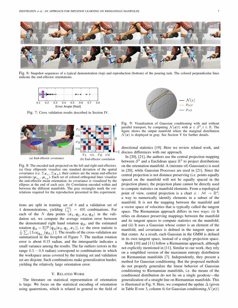
Fig. 6: Snapshot sequences of a typical demonstration (top) and reproduction (bottom) of the pouring task. The colored perpendicular linesindicate the end-effector orientations.

0.1 0.2 0.3 0.4 0.5 0.6 0.7 0.8

Error Angle [Rad]

Fig. 7: Cross validation results described in Section IV.

(a) End-effector covariance

xL xR

xL

xR

−1

0

1

(b) End-effector correlation

Fig. 8: The encoded task projected on the left and right end-effectors.(a) Gray ellipsoids visualize one standard deviation of the spatialcovariance (i.e. ΣXL

, ΣXR), their centers are the mean end-effector

positions (µxL, µxR

). Each set of colored orthogonal lines visualizethe end-effector mean orientation, its covariance is visualized by theellipses at the end of each axis. (b) Correlation encoded within andbetween the different manifolds. The gray rectangles mark the cor-relations required for the reproduction presented in this experiment.

tions are split in training set of 8 and a validation set of

4 demonstrations, yielding(

128

)

= 495 combinations. For

each of the N data points (xL, qL,xR, qR) in the vali-

dation set, we compute the average rotation error between

the demonstrated right hand rotation qR, and the estimated

rotation qR = E[P (qR|xR, qL,xL)], i.e. the error statistic is1N

∑

i ‖LogqR,i

(

qR,i

)

‖. The results of the cross-validation are

summarized in the boxplot of Figure 7. The median rotation

error is about 0.15 radian, and the interquartile indicates a

small variance among the results. The far outliers (errors in the

range 0.5− 0.8 radian) correspond to combinations in which

the workspace areas covered by the training set and validation

set are disjoint. Such combinations make generalization harder,

yielding the relatively large orientation error.

V. RELATED WORK

The literature on statistical representation of orientation

is large. We focus on the statistical encoding of orientation

using quaternions, which is related in general to the field of

Fig. 9: Visualization of Gaussian conditioning with and withoutparallel transport, by computing N (x|t) with x ∈ S2, t ∈ R. Thefigure shows the output manifold where the marginal distributionN (x) is displayed in gray. See Section V for further details.

directional statistics [19]. Here we review related work, and

discuss differences with our approach.

In [20], [21], the authors use the central projection mapping

between S3 and a Euclidean space R3 to project distributions

on the orientation manifold. A (mixture of) Gaussian(s) is used

in [20], while Gaussian Processes are used in [21]. Since the

central projection is not distance preserving (i.e. points equally

spaced on the manifold will not be equally spaced in the

projection plane), the projection plane cannot be directly used

to compute statistics on manifold elements. From a topological

point of view, central projection is a chart φ : M → Rd;

a way to numerically identify elements in a subset of the

manifold. It is not the mapping between the manifold and

a vector space of velocities that is typically called the tangent

space. The Riemannian approach differs in two ways: (i) It

relies on distance preserving mappings between the manifold

and its tangent spaces to compute statistics on the manifold;

and (ii) It uses a Gaussian whose center is an element of the

manifold, and covariance is defined in the tangent space at

that center. As a result, each Gaussian in the GMM is defined

in its own tangent space, instead of a single projection space.

Both [10] and [11] follow a Riemannian approach, although

not explicitly mentioned in [11]. Similar to our work, they rely

on a simplified version of the maximum entropy distribution

on Riemannian manifolds [7]. Independently, they present a

method for Gaussian conditioning. But the proposed methods

do not properly generalize the linear behavior of Gaussian

conditioning to Riemannian manifolds, i.e. the means of the

conditioned distribution do not lie on a single geodesic—the

generalization of a straight line on Riemannian manifolds. This

is illustrated in Fig. 9. Here, we computed the update ∆ (given

in Table II row 3, column 4) for Gaussian conditioning N (x|t)

8 IEEE ROBOTICS AND AUTOMATION LETTERS. PREPRINT VERSION. ACCEPTED JANUARY, 2017

with and without parallel transport, i.e. using Λ and Λ‖,

respectively. Without parallel transport the regression output

(solid blue line) does not lie on a geodesic, since it does not

coincide with the (unique) geodesic between the outer points

(dotted blue line). Using the proposed method that relies on

the parallel transported precision matrix Λ‖, the conditioned

means µ‖x|t (displayed in yellow) follow a geodesic path

on the manifold, thus generalizing the ‘linear’ behavior of

Gaussian conditioning to Riemannian manifolds.

Furthermore, the generalization of GMR proposed in [11]

relies on the weighted combination of quaternions presented

in [22]. Although this method seems to be widely accepted,

it skews the weighting of the quaternions. By applying this

method, one computes the chordal mean instead of the re-

quired weighted mean [23].

In general, the objective in probabilistic imitation learning is

to model behavior τ as the distribution P (τ). In this work we

take a direct approach and model a (mixture of) Gaussian(s)

over the state variables. Inverse Optimal Control (IOC) uses

a more indirect approach: it uses the demonstration data to

uncover an underlying cost function cθ(τ) parameterized by

θ. In [24], [25], pose information is learned by demonstration

by defining cost features for specific orientation and position

relationships between objects of interest and the robot end-

effector. An interesting parallel exists between our ‘direct’ ap-

proach and recent advances in IOC where behavior is modeled

as the maximum entropy distribution p(τ) = 1Zθ

exp(−cθ(τ))[26]–[28]. The Gaussian used in our work can be seen as an

approximation of this distribution, where the cost function is

the Mahalanobis distance defined on a Riemannian manifold.

The benefits of such an explicit cost structure are the ease of

finding the optimal reward (we learn its parameters through

EM), and the derivation of the policy (which we achieve

through conditioning).

VI. CONCLUSION

In this work we showed how a set of probabilistic imitation

learning techniques can be extended to Riemannian manifolds.

We described Gaussian conditioning, Gaussian Product and

parallel transport, which are the elementary tools required to

extend TP-GMM and GMR to Riemannian manifolds. The

selection of the Riemannian manifold approach is motivated

by the potential of extending the developed approach to other

Riemannian manifolds, and by the potential of drawing bridges

between other robotics challenges that involve a rich variety

of manifolds (including perception, planning and control prob-

lems).

REFERENCES

[1] K. P. Murphy, Machine Learning: A Probabilistic Perspective. TheMIT Press, 2012.

[2] A. G. Billard, S. Calinon, and R. Dillmann, “Learning from humans,”in Handbook of Robotics, B. Siciliano and O. Khatib, Eds. Secaucus,NJ, USA: Springer, 2016, ch. 74, pp. 1995–2014, 2nd Edition.

[3] A. Paraschos, C. Daniel, J. Peters, and G. Neumann, “Probabilisticmovement primitives,” in Advances in Neural Information ProcessingSystems (NIPS), 2013, pp. 2616–2624.

[4] S. Calinon, “A tutorial on task-parameterized movement learning andretrieval,” Intelligent Service Robotics, vol. 9, no. 1, pp. 1–29, January2016.

[5] J. Silverio, L. Rozo, S. Calinon, and D. G. Caldwell, “Learning bimanualend-effector poses from demonstrations using task-parameterized dy-namical systems,” in Proc. IEEE/RSJ Intl Conf. on Intelligent Robotsand Systems (IROS), 2015, pp. 464–470.

[6] R. Hosseini and S. Sra, “Matrix manifold optimization for Gaussian mix-tures,” in Advances in Neural Information Processing Systems (NIPS),2015, pp. 910–918.

[7] X. Pennec, “Intrinsic statistics on Riemannian manifolds: Basic tools forgeometric measurements,” Journal of Mathematical Imaging and Vision,vol. 25, no. 1, pp. 127–154, 2006.

[8] N. Ratliff, M. Toussaint, and S. Schaal, “Understanding the geometry ofworkspace obstacles in motion optimization,” in Proc. IEEE Intl Conf.on Robotics and Automation (ICRA), 2015, pp. 4202–4209.

[9] S. Hauberg, O. Freifeld, and M. J. Black, “A geometric take onmetric learning,” in Advances in Neural Information Processing Systems(NIPS), 2012, pp. 2024–2032.

[10] E. Simo-Serra, C. Torras, and F. Moreno-Noguer, “3D Human PoseTracking Priors using Geodesic Mixture Models,” International Journalof Computer Vision (IJCV), pp. 1–21, August 2016.

[11] S. Kim, R. Haschke, and H. Ritter, “Gaussian mixture model for 3-doforientations,” Robotics and Autonomous Systems, vol. 87, pp. 28 – 37,October 2017.

[12] P.-A. Absil, R. Mahony, and R. Sepulchre, Optimization Algorithms onMatrix Manifolds. Princeton, NJ: Princeton University Press, 2008.

[13] G. Dubbelman, “Intrinsic statistical techniques for robust pose estima-tion,” Ph.D. dissertation, University of Amsterdam, September 2011.

[14] S. M. Khansari-Zadeh and A. Billard, “Learning stable non-lineardynamical systems with Gaussian mixture models,” IEEE Trans. onRobotics, vol. 27, no. 5, pp. 943–957, 2011.

[15] S. Calinon, D. Bruno, and D. G. Caldwell, “A task-parameterizedprobabilistic model with minimal intervention control,” in Proc. IEEEIntl Conf. on Robotics and Automation (ICRA), 2014, pp. 3339–3344.

[16] O. Freifeld, S. Hauberg, and M. J. Black, “Model transport: Towardsscalable transfer learning on manifolds,” in Proceedings IEEE Conf. onComputer Vision and Pattern Recognition (CVPR), 2014, pp. 1378 –1385.

[17] B. B. Ready, “Filtering techniques for pose estimation with applica-tions to unmanned air vehicles,” Ph.D. dissertation, Brigham YoungUniversity-Provo, November 2012.

[18] S. Hauberg, F. Lauze, and K. S. Pedersen, “Unscented Kalman filteringon Riemannian manifolds,” Journal of mathematical imaging and vision,vol. 46, no. 1, pp. 103–120, 2013.

[19] K. V. Mardia and P. E. Jupp, Directional statistics. John Wiley & Sons,2009, vol. 494.

[20] W. Feiten, M. Lang, and S. Hirche, “Rigid Motion Estimation usingMixtures of Projected Gaussians,” in 16th International Conference onInformation Fusion (FUSION), 2013, pp. 1465–1472.

[21] M. Lang, M. Kleinsteuber, O. Dunkley, and S. Hirche, “Gaussianprocess dynamical models over dual quaternions,” in European ControlConference (ECC), 2015, pp. 2847–2852.

[22] F. L. Markley, Y. Cheng, J. L. Crassidis, and Y. Oshman, “Averaging qua-terions,” Journal of Guidance, Control, and Dynamics (AIAA), vol. 30,pp. 1193–1197, July 2007.

[23] R. I. Hartley, J. Trumpf, Y. Dai, and H. Li, “Rotation averaging,”International Journal of Computer Vision, vol. 103, no. 3, pp. 267–305,July 2013.

[24] P. Englert and M. Toussaint, “Inverse KKT–learning cost functionsof manipulation tasks from demonstrations,” in Proc. Intl Symp. onRobotics Research (ISRR), 2015.

[25] A. Doerr, N. Ratliff, J. Bohg, M. Toussaint, and S. Schaal, “Directloss minimization inverse optimal control,” in Proceedings of Robotics:Science and Systems (RSS), 2015, pp. 1–9.

[26] B. D. Ziebart, A. L. Maas, J. A. Bagnell, and A. K. Dey, “Maximum en-tropy inverse reinforcement learning.” in AAAI Conference on ArtificialIntelligence, 2008, pp. 1433–1438.

[27] S. Levine and V. Koltun, “Continuous inverse optimal control withlocally optimal examples,” in Proceedings of the 29th InternationalConference on Machine Learning (ICML), July 2012, pp. 41–48.

[28] C. Finn, S. Levine, and P. Abbeel, “Guided cost learning: Deep in-verse optimal control via policy optimization,” in Proceedings of 33rdInternational Conference on Machine Learning (ICML), June 2016, pp.49–58.