An approach to feature location in distributed systems

www.elsevier.com/locate/jss

The Journal of Systems and Software 79 (2006) 57–68

An approach to feature location in distributed systems

Dennis Edwards, Sharon Simmons, Norman Wilde *

Department of Computer Science, University of West Florida, 11000 University Parkway, Pensacola, FL 32514, USA

Received 11 March 2004; received in revised form 20 December 2004; accepted 24 December 2004Available online 20 January 2005

Abstract

This paper describes an approach to the feature location problem for distributed systems, that is, to the problem of locating whichcode components are important in providing a particular feature for an end user. A feature is located by observing system executionand noting time intervals in which it is active. Traces of execution in intervals with and without the feature are compared. Earlierexperience has shown that this analysis is difficult because distributed systems often exhibit stochastic behavior and because timeintervals are hard to identify with precision.

To get around these difficulties, the paper proposes a definition of time interval based on the causality analysis introduced byLamport and others. A strict causal interval may be defined, but it must often be extended to capture latent events and to representthe inherent imprecision in time measurement. This extension is modeled using a weighting function which may be customized to thespecific circumstances of each study.

The end result of the analysis is a component relevance index, denoted pc, which can be used to measure the relevance of a softwarecomponent to a particular feature. Software engineers may focus their analysis efforts on the top components as ranked according topc.

Two case studies are presented. The first study demonstrates the feasibility of pc by applying our method to a well-defined dis-tributed system. The second study demonstrates the versatility of pc by applying our method to message logs obtained from a largemilitary system. Both studies indicate that the suggested approach could be an effective guide for a software engineer who is main-taining or enhancing a distributed system.� 2005 Elsevier Inc. All rights reserved.

Keywords: Feature location; Distributed systems; Software reconnaissance

1. Introduction

Software engineers who deal with complex softwareare often faced with the problem of locating where spe-cific features of a program are implemented. Featuresare services that the software provides to its users andare usually described in terms appropriate to the prob-lem domain in which the software operates. For exam-ple, product literature for a word processor would

0164-1212/$ - see front matter � 2005 Elsevier Inc. All rights reserved.doi:10.1016/j.jss.2004.12.018

* Corresponding author. Tel.: +1 850 474 2542; fax: +1 850 8576056.

E-mail addresses: [email protected] (D. Edwards), [email protected] (S. Simmons), [email protected] (N. Wilde).

mention features for entering and editing text, movingthe cursor, setting and changing fonts, printing, and sav-ing the resulting file in numerous formats.

The software engineer, in making enhancements orrepairing faults, works with the program as a collectionof software components: at a high level these are modulesand object classes; at a lower level they are subroutinesand data items; at the lowest level they may be individ-ual lines of code. However the tasks the software engi-neer is assigned are often stated in feature terms. Hemay be asked, for example, to add a ‘‘bookmark facil-ity’’ to the word processor, a new user feature which willrequire understanding the editor and cursor moving fea-tures of the existing code.

mailto:[email protected]




58 D. Edwards et al. / The Journal of Systems and Software 79 (2006) 57–68

Unfortunately, user features rarely map cleanly ontosoftware components, especially in a large system whichhas been worked on by many hands. Thus software engi-neers are faced with the feature location problem: given afeature stated in user terms, how do I locate the softwarecomponents most intimately involved?

There has been some study of the feature locationproblem for sequential software, but very little workhas been done in the distributed domain. One would ex-pect that the need for effective techniques of featurelocation will be even greater in the distributed world,given the added complexities introduced by distribution,concurrency, and timing effects.

In this paper we first describe the approaches to fea-ture location that have been proposed for sequentialsoftware. We then describe an early attempt to applyone of these methods to Joint STARS, a real, large scale,distributed system, and some of the difficulties that wereencountered. Drawing on this experience, we describe anew approach to address these problems based on theconcept of causality developed by Lamport and others.We provide some results from a small scale case studyto explore the feasibility of the approach. Finally, we re-visit the Joint STARS data to see how our approachmight have been usable in that real-world case.

2. The feature location problem in sequential systems

As a practical matter, it has long been clear that soft-ware engineers dealing with an industrial-scale softwaresystem can rarely afford themselves the luxury of under-standing it completely. Instead they adopt an as-neededstrategy of locating the most relevant software compo-nents and understanding these as well as they can(Koenemann and Robertson, 1991).

The problem is, of course, the location of the relevantcomponents in the hundreds of thousands of lines thatmake up a real system. Early work by Weiser (1982)introduced the concept of program slicing. A programslice is an executable subset of a program computed stat-ically according to some criterion. In the most commonexample, a slice is taken on a particular variable at aparticular point in the code, and consists of all programstatements needed to compute the value of that variableat that point. Classical slicing can be a very powerfultechnique, but it requires a program variable as a start-ing point; there may be no easy way to identify a specificvariable that corresponds to a user-described feature. Aswell, the slice often turns out to be a large proportion ofthe original program.

Other authors have also described static analysis ap-proaches to locating software components. Biggerstaffet. al. conceptualized the program as concept assignment,and described the DESIRE tool which uses a combina-tion of parsing, clustering, and the analysis of data items

and their names (Biggerstaff et al., 1994). More recentlyChen and Rajlich (2000) described a static approachwhich involves systematic manual search through theprogram�s dependency graph to locate relevant codeand data items.

In practice, software engineers most often attempt tolocate features by text search with tools such as grep

(Sim et al., 1998). Text search looks for code commentsor variable names associatedwith a feature. Text searchinghas the advantage of being very fast and easy to use, but forsuccess requires both good comments or variable namesand the use of exactly the same vocabulary as that of theoriginal programmer. The search for a ‘‘font change’’ fea-ture would fail, for example, if the code comment con-tained ‘‘typeface change’’ instead of ‘‘font change’’.

Dynamic analysis techniques have shown great poten-tial for feature location, since they involve observing thecode as the feature of interest is performed. The best-known technique of this sort is software reconnaissance, de-scribed byWilde and Scully (1995) and further formalizedby Deprez and Lakhotia (2000). The technique requiresrunning the system for several test cases, including somewhich perform the feature and others which do not. Inits simplest form, the analysis takes the set of softwarecomponents executed in tests with the feature and sub-tracts the set of such components executed in the remain-ing tests. The result is a relatively small set of marker

components for the feature. Other authors have suggestedother heuristics to locate wider or narrower sets of feature-related software components (Wong et al., 1999b).

There have been several published case studies thatapply such dynamic analysis techniques to different pro-grams (Wilde and Casey, 1996; Agrawal et al., 1998;Wong et al., 1999b; Wilde et al., 2001) and several toolsare available (Wilde, 2003; Telecordia Technologies,Inc., 2003). The general consensus seems to be that suchtechniques are effective in focusing on a relatively smallfraction of the code that needs to be examined to under-stand the feature. The marker code by itself is not suffi-cient since it needs to be put into context before it can beunderstood, but these techniques provide good startingpoints for efficient code exploration.

A somewhat different dynamic analysis approach hasbeen described by Eisenbarth et al. (2002). They also col-lect traces of subroutine calls as the program is executedfor a series of scenarios, each one of which is tagged withthe features it involves. The traces are analyzed to catego-rize subroutines according to their degree of specificity toa given feature. The analysis also automatically producesa set of concepts for the program. The concepts are sub-sets of the subroutines that tend to execute togetherand are presented organized in a lattice. A case studyhas showed that the concepts and the lattice may provideuseful insight into the design of the system.

Finally, Wong et al. (1999a) have extended the dy-namic analysis methods to quantify feature location.

D. Edwards et al. / The Journal of Systems and Software 79 (2006) 57–68 59

They developed metrics based on execution slices of theprogram, and used them to measure the disparity be-tween a feature and a component, the concentration ofa feature in a component, and the dedication of a com-ponent to a feature.

3. Joint STARS—an early case study

Little work has been done on methods for locatingfeatures in distributed systems. Much of the motivationfor the current research was a study performed in 1996on a large military distributed system called Joint

STARS (Wilde et al., 1998). Joint STARS is an airbornebattle management system developed by NorthropGrumman Corporation for the US Air Force in supportof the US Army. It consists of a militarized Boeing 707aircraft with an advanced radar system and mobileground stations. Operators in the aircraft provide tar-geting data both to other aircraft and to ground units(Northrop Grumman, 2004). The Joint STARS contrac-tor-developed software consisted of approximately 360thousand lines of code running as 233 processes on avariable number of processors.

The study applied a variant of the software recon-naissance method for design recovery, that is, to recoverinformation about the as-built design from the finishedsoftware. Joint STARS was originally designed, in part,using the concept of design threads. A design threadshowed the expected interactions between the differentprocesses when a particular feature was invoked, forexample, by the operator in the aircraft selecting a par-ticular function. The design threads were represented asdata flow diagrams showing the processes, inter-processmessages, and data stores expected to be involved in thefeature. The purpose of the study was to recover a sam-ple of the as-built design threads, which might be ex-pected to differ somewhat from the originals. It wasanticipated that recovered design threads could be usefulin maintaining the software, especially since some turn-over of personnel was anticipated.

The input for the study consisted of logs of JointSTARS inter-process messages which were availableusing debugging facilities built in to the system. Thelogged data for each message included an approximatetime stamp, the message source, the message destina-tion, and the message type. Start and end times for fivedifferent features were noted by hand and compared tothe logged time stamps to identify the log entries duringeach feature execution. The log during feature executionwas compared to the log in system idle periods to findmarker messages using the set difference method de-scribed in the previous section.

While the study was successful in recovering severalthreads, some difficulties were encountered. First, thetheory of software reconnaissance had always been sta-

ted as taking the set difference between execution tracesof test cases. The implicit assumption is that a test casehas a clearly defined start and end. However for JointSTARS, as for most distributed systems, the softwarerarely really starts and stops—it runs continuously whileoperators invoke different features. It is difficult to reg-ister exact start and stop times. As well, logged timestamps themselves might not be strictly comparable be-cause clocks on different processors are not preciselysynchronized. In fact, two of the five data sets in thestudy had to be discarded because start and stop timeswere not determined precisely enough.

Second, Joint STARS did not always execute exactlythe same way during a feature. Each feature was exe-cuted three times, but some messages appeared in onlyone or two of the relevant logs. The problem seemedto stem from the occurrence of timed events which hap-pened to occur during the feature�s execution. It wasalso possible that message logging occasionally lost dataas buffers filled up. The software reconnaissance meth-od, based on simple set differences between the logs, pro-vided no clear way of handling such problems.

In general, practical analysis of traces in a distributedsystem must take into account difficulties of observationof time, as well as behavior in the system itself which iseffectively stochastic. These problems are well known totesters of such systems (Schutz, 1994). Thus the estab-lished dynamic analysis methods for feature locationare not complete when applied to distributed systems.

To recapitulate, the goal is to provide a mapping be-tween a feature and the key software components involvedin its implementation. The mapping givesmarker compo-nents for each feature and would be used to give a soft-ware engineer starting points for code exploration intrying to understand it. For our purposes a feature isany episodically occurring service provided to a user.The user may choose to define the system�s features inany way he chooses, provided only that he can identifywhen each feature occurs and when it does not. Featuresare most commonly initiated by user input but even a bugmay be thought of as a feature if it is observable and iden-tifiable. We exclude only services that are always per-formed, independent of user input or observation.

The definition of software component is likewise flex-ible. Software components may be classes, individualobjects, subroutines, specific lines of code, or even mes-sage types. The only restriction is that it must be possi-ble to instrument the software so that we can observewhen each component is used.

If a software component�s executions tend to occur atnearly the same time as occurrences of a feature, thenthe component is likely to be feature related. The closerthis time relationship, the more likely that we havefound a key component to investigate.

For distributed systems, the key to the dynamic loca-tion methods is thus time. Unfortunately, the concept of


a time interval in a distributed system is not straightfor-ward. It is not trivial to determine if a particular compo-nent�s execution occurred after the start of a feature andbefore its end because the correct ordering of events ondifferent processes may be indeterminate. Event timestamps are not sufficient since it is generally not possibleto guarantee that clocks will be closely synchronized.These difficulties add to the problem of stochasticbehavior and will be addressed in the next section.

4. System model and time intervals

A distributed system may be modeled as a set, C, ofsoftware components. The definition of a software com-ponent is intentionally left nebulous to allow explora-tion of the system from the fine grained, statementlevel to the course-grained modular level.

C ¼ fc1; c2; . . . ; cq; . . . ; cQg ð1ÞWe let F denote the feature the software engineer is

investigating.Fundamental to our research is the association

between events of a distributed system�s execution andthe components of the distributed system. An event isa discrete occurrence on a process. As software compo-nents execute, they generate events in the N differentprocesses of the system, P1, . . . ,PN. The events on pro-cess Pi are identified by the set Ei.

Ei ¼ fe1i ; e2i ; . . . ; eki ; . . .g ð2ÞThe set E contains all events in the system and is theunion of the events from each individual process.

E ¼ E1 [ E2 [ � � � [ EN ð3ÞA software component, cq, is the source of an event, eki , ifevent eki was the direct result of the execution of cq. Thefunction d( ) maps the event to the source component.

cq ¼ dðeki Þ ð4ÞWhile each event will map onto a single component, theinverse does not hold. For example if a component isexecuted in a loop it will produce a unique event eachtime it is executed. All of these events will map backto the single component through function d( ).

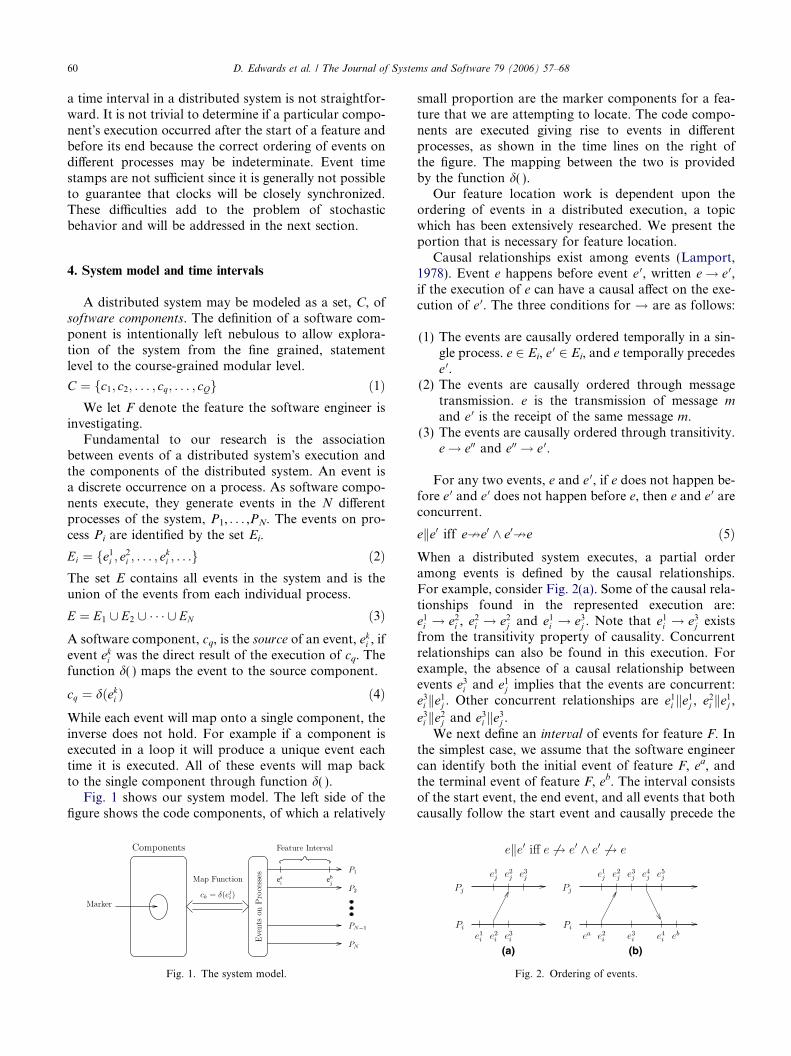
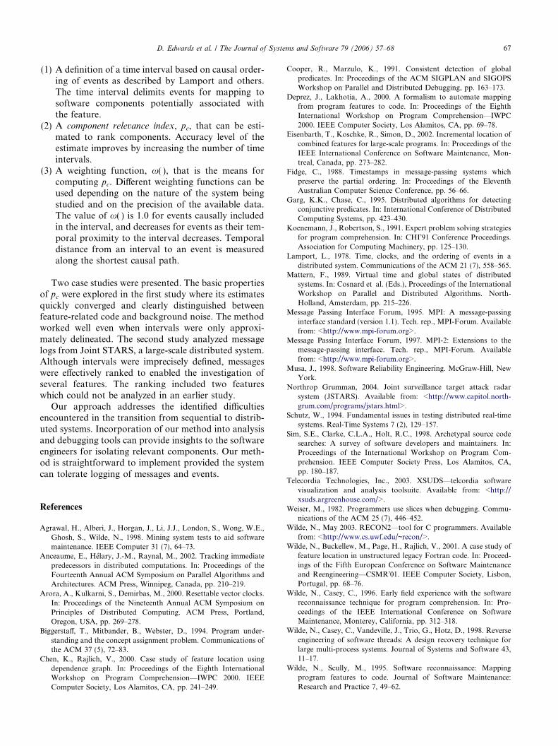
Fig. 1 shows our system model. The left side of thefigure shows the code components, of which a relatively

Fig. 1. The system model.

small proportion are the marker components for a fea-ture that we are attempting to locate. The code compo-nents are executed giving rise to events in differentprocesses, as shown in the time lines on the right ofthe figure. The mapping between the two is providedby the function d( ).

Our feature location work is dependent upon theordering of events in a distributed execution, a topicwhich has been extensively researched. We present theportion that is necessary for feature location.

Causal relationships exist among events (Lamport,1978). Event e happens before event e 0, written e ! e 0,if the execution of e can have a causal affect on the exe-cution of e 0. The three conditions for ! are as follows:

(1) The events are causally ordered temporally in a sin-gle process. e 2 Ei, e

0 2 Ei, and e temporally precedese 0.

(2) The events are causally ordered through messagetransmission. e is the transmission of message m

and e 0 is the receipt of the same message m.(3) The events are causally ordered through transitivity.

e ! e00 and e00 ! e 0.

For any two events, e and e 0, if e does not happen be-fore e 0 and e 0 does not happen before e, then e and e 0 areconcurrent.

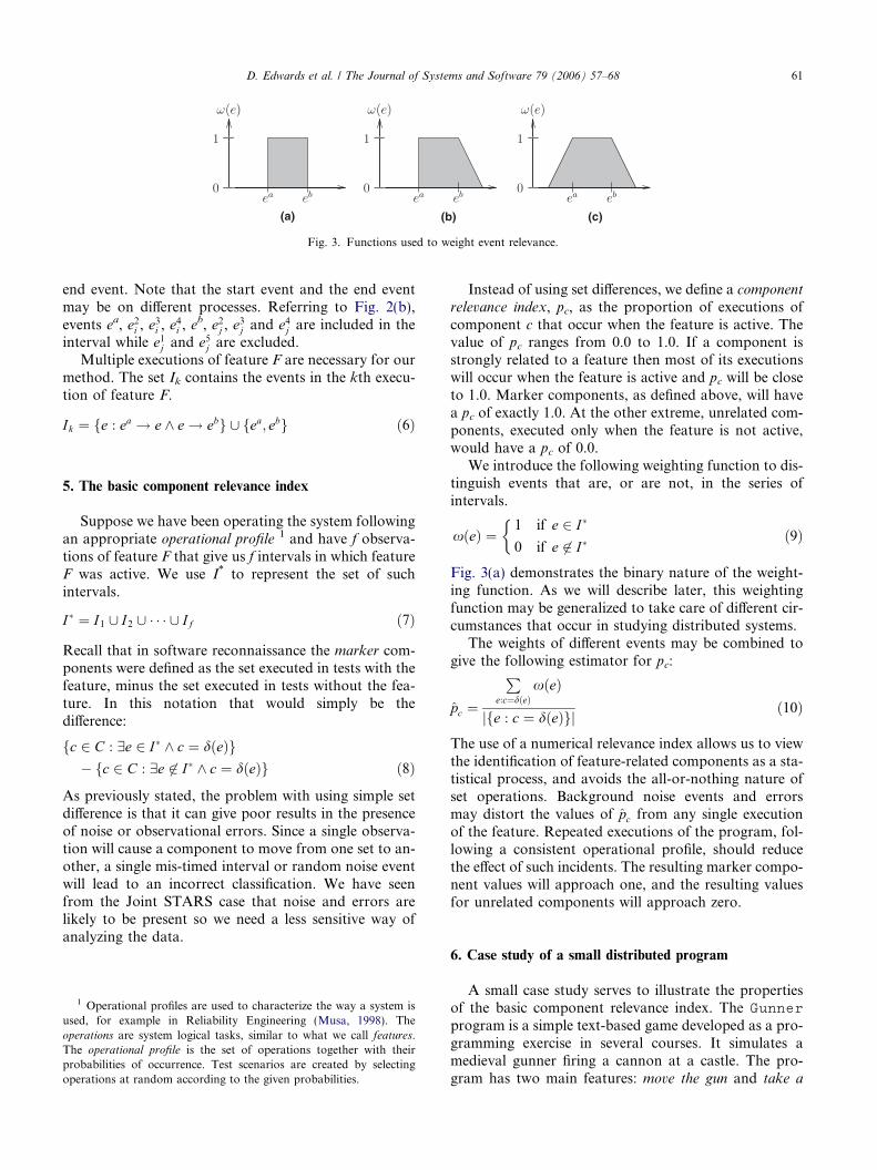
eke0 iff e9e0 ^ e09e ð5ÞWhen a distributed system executes, a partial orderamong events is defined by the causal relationships.For example, consider Fig. 2(a). Some of the causal rela-tionships found in the represented execution are:e1i ! e2i , e

2i ! e2j and e1i ! e3j . Note that e1i ! e3j exists

from the transitivity property of causality. Concurrentrelationships can also be found in this execution. Forexample, the absence of a causal relationship betweenevents e3i and e1j implies that the events are concurrent:e3i ke1j . Other concurrent relationships are e1i ke1j , e2i ke1j ,e3i ke2j and e3i ke3j .

We next define an interval of events for feature F. Inthe simplest case, we assume that the software engineercan identify both the initial event of feature F, ea, andthe terminal event of feature F, eb. The interval consistsof the start event, the end event, and all events that bothcausally follow the start event and causally precede the

(a) (b)

Fig. 2. Ordering of events.

(a) (b) (c)

Fig. 3. Functions used to weight event relevance.


end event. Note that the start event and the end eventmay be on different processes. Referring to Fig. 2(b),events ea, e2i , e

3i , e

4i , e

b, e2j , e3j and e4j are included in the

interval while e1j and e5j are excluded.Multiple executions of feature F are necessary for our

method. The set Ik contains the events in the kth execu-tion of feature F.

Ik ¼ fe : ea ! e ^ e ! ebg [ fea; ebg ð6Þ

5. The basic component relevance index

Suppose we have been operating the system followingan appropriate operational profile 1 and have f observa-tions of feature F that give us f intervals in which featureF was active. We use I* to represent the set of suchintervals.

I� ¼ I1 [ I2 [ � � � [ If ð7Þ

Recall that in software reconnaissance the marker com-ponents were defined as the set executed in tests with thefeature, minus the set executed in tests without the fea-ture. In this notation that would simply be thedifference:

fc 2 C : 9e 2 I� ^ c ¼ dðeÞg� fc 2 C : 9e 62 I� ^ c ¼ dðeÞg ð8Þ

As previously stated, the problem with using simple setdifference is that it can give poor results in the presenceof noise or observational errors. Since a single observa-tion will cause a component to move from one set to an-other, a single mis-timed interval or random noise eventwill lead to an incorrect classification. We have seenfrom the Joint STARS case that noise and errors arelikely to be present so we need a less sensitive way ofanalyzing the data.

1 Operational profiles are used to characterize the way a system isused, for example in Reliability Engineering (Musa, 1998). Theoperations are system logical tasks, similar to what we call features.The operational profile is the set of operations together with theirprobabilities of occurrence. Test scenarios are created by selectingoperations at random according to the given probabilities.

Instead of using set differences, we define a component

relevance index, pc, as the proportion of executions ofcomponent c that occur when the feature is active. Thevalue of pc ranges from 0.0 to 1.0. If a component isstrongly related to a feature then most of its executionswill occur when the feature is active and pc will be closeto 1.0. Marker components, as defined above, will havea pc of exactly 1.0. At the other extreme, unrelated com-ponents, executed only when the feature is not active,would have a pc of 0.0.

We introduce the following weighting function to dis-tinguish events that are, or are not, in the series ofintervals.

xðeÞ ¼1 if e 2 I�

0 if e 62 I�

�ð9Þ

Fig. 3(a) demonstrates the binary nature of the weight-ing function. As we will describe later, this weightingfunction may be generalized to take care of different cir-cumstances that occur in studying distributed systems.

The weights of different events may be combined togive the following estimator for pc:

pc ¼

Pe:c¼dðeÞ

xðeÞ

jfe : c ¼ dðeÞgj ð10Þ

The use of a numerical relevance index allows us to viewthe identification of feature-related components as a sta-tistical process, and avoids the all-or-nothing nature ofset operations. Background noise events and errorsmay distort the values of pc from any single executionof the feature. Repeated executions of the program, fol-lowing a consistent operational profile, should reducethe effect of such incidents. The resulting marker compo-nent values will approach one, and the resulting valuesfor unrelated components will approach zero.

6. Case study of a small distributed program

A small case study serves to illustrate the propertiesof the basic component relevance index. The Gunner

program is a simple text-based game developed as a pro-gramming exercise in several courses. It simulates amedieval gunner firing a cannon at a castle. The pro-gram has two main features: move the gun and take a

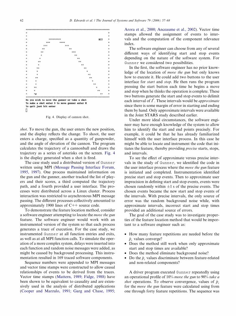
Fig. 4. Display of cannon shot.


shot. To move the gun, the user enters the new position,and the display reflects the change. To shoot, the userenters a charge, specified as a quantity of gunpowder,and the angle of elevation of the cannon. The programcalculates the trajectory of a cannonball and draws thetrajectory as a series of asterisks on the screen. Fig. 4is the display generated when a shot is fired.

The case study used a distributed version of Gunnerwritten using MPI (Message Passing Interface Forum,1995, 1997). One process maintained information onthe gun and the gunner, another tracked the list of play-ers and their scores, a third computed the trajectorypath, and a fourth provided a user interface. The pro-cesses were distributed across a Linux cluster. Processinteraction was restricted to asynchronous MPI messagepassing. The different processes collectively amounted toapproximately 1900 lines of C++ source code.

To demonstrate the feature location method, considera software engineer attempting to locate themove the gun

feature. The software engineer would work with aninstrumented version of the system so that each processgenerates a trace of execution. For the case study, weinstrumented Gunner at all function entries and exits,as well as at all MPI function calls. To simulate the oper-ation of a more complex system, delays were inserted intoeach function and random noise messages were added, asmight be caused by background processing. This instru-mentation resulted in 169 traced software components.

Sequence numbers were appended to MPI messagesand vector time stamps were constructed to allow causalrelationships of events to be derived from the traces.Vector time stamps (Mattern, 1989; Fidge, 1988) havebeen shown to be equivalent to causality and are exten-sively used in the analysis of distributed applications(Cooper and Marzulo, 1991; Garg and Chase, 1995;

Arora et al., 2000; Anceaume et al., 2002). Vector timestamps allowed the assignment of events to inter-vals and the computation of the component relevanceindex.

The software engineer can choose from any of severaldifferent ways of identifying start and stop eventsdepending on the nature of the software system. ForGunner we considered two possibilities.

In the first, the software engineer has no prior know-ledge of the location of move the gun but only knowshow to execute it. He could add two buttons to the userinterface for start and stop. He then runs the programpressing the start button each time he begins a moveand stop when he thinks the operation is complete. Thesetwo buttons generate the start and stop events to delimiteach interval of I*. These intervals would be approximate

since there is some margin of error in starting and endingthem by hand. Only approximate intervals were availablein the Joint STARS study described earlier.

Under more ideal circumstances, the software engi-neer may have enough knowledge of the system to allowhim to identify the start and end points precisely. Forexample, it could be that he has already familiarizedhimself with the user interface process. In this case hemight be able to locate and instrument the code that ini-tiates the feature, thereby providing precise starts, stops,and intervals.

To see the effect of approximate versus precise inter-vals in the study of Gunner, we identified the code inthe user interface process where the move the gun featureis initiated and completed. Instrumentation identifiedprecise start and stop events. Then to approximate userimprecision in defining start and stop events, events werechosen randomly within ±1 s of the precise events. Thechosen events became the new start and stop events ofthe intervals. With precise intervals, the only source oferror was the random background noise while, withapproximate intervals, incorrect start and stop timesprovided an additional source of errors.

The goal of the case study was to investigate proper-ties of the feature location method that would be impor-tant to a software engineer such as:

• How many feature repetitions are needed before thepc values converge?

• Does the method still work when only approximatestart and stop times are available?

• Does the method eliminate background noise?• Do the pc values discriminate between feature-related

and non-related components?

A driver program executed Gunner repeatedly usingan operational profile of 10% move the gun to 90% take a

shot operations. To observe convergence, values of pcfor the move the gun feature were calculated using fromone through forty feature repetitions. The sequence was

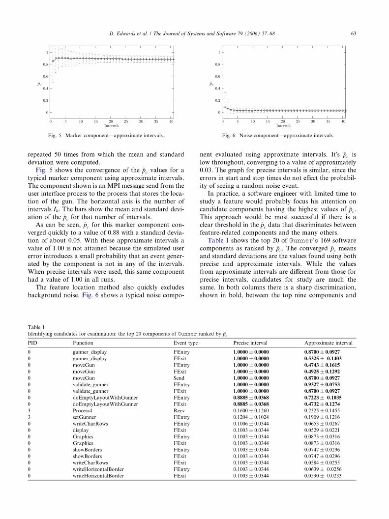
Fig. 5. Marker component—approximate intervals. Fig. 6. Noise component—approximate intervals.


repeated 50 times from which the mean and standarddeviation were computed.

Fig. 5 shows the convergence of the pc values for atypical marker component using approximate intervals.The component shown is an MPI message send from theuser interface process to the process that stores the loca-tion of the gun. The horizontal axis is the number ofintervals Ik. The bars show the mean and standard devi-ation of the pc for that number of intervals.

As can be seen, pc for this marker component con-verged quickly to a value of 0.88 with a standard devia-tion of about 0.05. With these approximate intervals avalue of 1.00 is not attained because the simulated usererror introduces a small probability that an event gener-ated by the component is not in any of the intervals.When precise intervals were used, this same componenthad a value of 1.00 in all runs.

The feature location method also quickly excludesbackground noise. Fig. 6 shows a typical noise compo-

Table 1Identifying candidates for examination: the top 20 components of Gunner

PID Function Event type

0 gunner_display FEntry0 gunner_display FExit0 moveGun FEntry0 moveGun FExit0 moveGun Send0 validate_gunner FEntry0 validate_gunner FExit0 doEmptyLayoutWithGunner FEntry0 doEmptyLayoutWithGunner FExit3 Process4 Recv3 setGunner FEntry0 writeCharRows FEntry0 display FExit0 Graphics FEntry0 Graphics FExit0 showBorders FEntry0 showBorders FExit0 writeCharRows FExit0 writeHorizontalBorder FEntry0 writeHorizontalBorder FExit

nent evaluated using approximate intervals. It�s pc islow throughout, converging to a value of approximately0.03. The graph for precise intervals is similar, since theerrors in start and stop times do not effect the probabil-ity of seeing a random noise event.

In practice, a software engineer with limited time tostudy a feature would probably focus his attention oncandidate components having the highest values of pc.This approach would be most successful if there is aclear threshold in the pc data that discriminates betweenfeature-related components and the many others.

Table 1 shows the top 20 of Gunner�s 169 softwarecomponents as ranked by pc. The converged pc meansand standard deviations are the values found using bothprecise and approximate intervals. While the valuesfrom approximate intervals are different from those forprecise intervals, candidates for study are much thesame. In both columns there is a sharp discrimination,shown in bold, between the top nine components and

ranked by pc

Precise interval Approximate interval

1.0000 ± 0.0000 0.8700 ± 0.0927

1.0000 ± 0.0000 0.5325 ± 0.1403

1.0000 ± 0.0000 0.4743 ± 0.1615

1.0000 ± 0.0000 0.4925 ± 0.1292

1.0000 ± 0.0000 0.8700 ± 0.0927

1.0000 ± 0.0000 0.9327 ± 0.0753

1.0000 ± 0.0000 0.8700 ± 0.0927

0.8885 ± 0.0368 0.7223 ± 0.1035

0.8885 ± 0.0368 0.4732 ± 0.1274

0.1600 ± 0.1260 0.2325 ± 0.14550.1204 ± 0.1024 0.1909 ± 0.12160.1006 ± 0.0344 0.0653 ± 0.02670.1003 ± 0.0344 0.0529 ± 0.02210.1003 ± 0.0344 0.0873 ± 0.03160.1003 ± 0.0344 0.0873 ± 0.03160.1003 ± 0.0344 0.0747 ± 0.02960.1003 ± 0.0344 0.0747 ± 0.02960.1003 ± 0.0344 0.0584 ± 0.02550.1003 ± 0.0344 0.0639 ± 0.02560.1003 ± 0.0344 0.0590 ± 0.0233


the remainder. For precise intervals the threshold comesat a pc value of 0.88 while with approximate intervals itis at 0.47. In either case, a software engineer wouldprobably look at the sudden drop after this point as asignal to concentrate his attention on the top 9 to under-stand the move the gun feature.

A quick check of these components in the Gunner

code shows that the top nine are, in fact, heavily usedin the move the gun feature.

While results from this small case study may not, ofcourse, generalize to full scale distributed systems, atleast in this example the pc method converged fairly rap-idly, excluded noise events clearly, and was robust in thepresence of noise and user errors. It identified a manage-ably small set of components (9 out of 169) for furtherstudy by the software engineer.

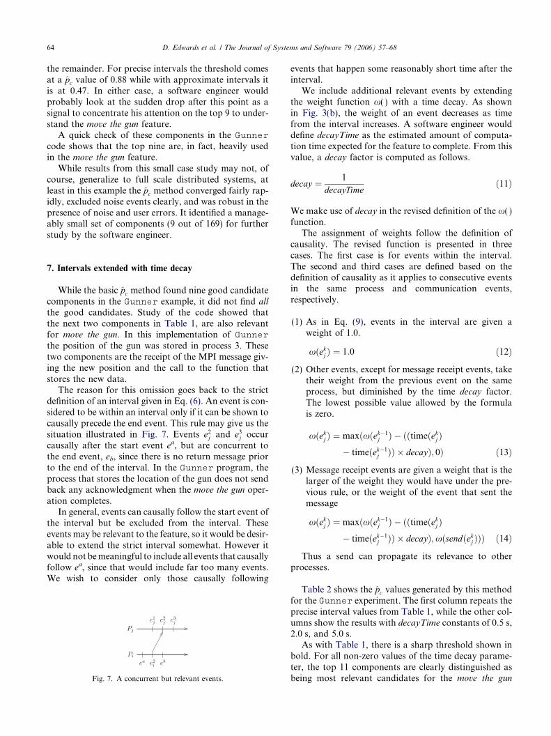
7. Intervals extended with time decay

While the basic pc method found nine good candidatecomponents in the Gunner example, it did not find allthe good candidates. Study of the code showed thatthe next two components in Table 1, are also relevantfor move the gun. In this implementation of Gunner

the position of the gun was stored in process 3. Thesetwo components are the receipt of the MPI message giv-ing the new position and the call to the function thatstores the new data.

The reason for this omission goes back to the strictdefinition of an interval given in Eq. (6). An event is con-sidered to be within an interval only if it can be shown tocausally precede the end event. This rule may give us thesituation illustrated in Fig. 7. Events e2j and e3j occurcausally after the start event ea, but are concurrent tothe end event, eb, since there is no return message priorto the end of the interval. In the Gunner program, theprocess that stores the location of the gun does not sendback any acknowledgment when the move the gun oper-ation completes.

In general, events can causally follow the start event ofthe interval but be excluded from the interval. Theseevents may be relevant to the feature, so it would be desir-able to extend the strict interval somewhat. However itwould not bemeaningful to include all events that causallyfollow ea, since that would include far too many events.We wish to consider only those causally following

Fig. 7. A concurrent but relevant events.

events that happen some reasonably short time after theinterval.

We include additional relevant events by extendingthe weight function x( ) with a time decay. As shownin Fig. 3(b), the weight of an event decreases as timefrom the interval increases. A software engineer woulddefine decayTime as the estimated amount of computa-tion time expected for the feature to complete. From thisvalue, a decay factor is computed as follows.

decay ¼ 1

decayTimeð11Þ

We make use of decay in the revised definition of the x( )function.

The assignment of weights follow the definition ofcausality. The revised function is presented in threecases. The first case is for events within the interval.The second and third cases are defined based on thedefinition of causality as it applies to consecutive eventsin the same process and communication events,respectively.

(1) As in Eq. (9), events in the interval are given aweight of 1.0.

xðekj Þ ¼ 1:0 ð12Þ

(2) Other events, except for message receipt events, taketheir weight from the previous event on the sameprocess, but diminished by the time decay factor.The lowest possible value allowed by the formulais zero.

xðekj Þ ¼ maxðxðek�1j Þ � ððtimeðekj Þ

� timeðek�1j ÞÞ � decayÞ; 0Þ ð13Þ

(3) Message receipt events are given a weight that is thelarger of the weight they would have under the pre-vious rule, or the weight of the event that sent themessage

xðekj Þ ¼ maxðxðek�1j Þ � ððtimeðekj Þ

� timeðek�1j ÞÞ � decayÞ;xðsendðekj ÞÞÞ ð14Þ

Thus a send can propagate its relevance to otherprocesses.

Table 2 shows the pc values generated by this methodfor the Gunner experiment. The first column repeats theprecise interval values from Table 1, while the other col-umns show the results with decayTime constants of 0.5 s,2.0 s, and 5.0 s.

As with Table 1, there is a sharp threshold shown inbold. For all non-zero values of the time decay parame-ter, the top 11 components are clearly distinguished asbeing most relevant candidates for the move the gun

Table 2Identifying components in Gunner using pc values for different decay times

PID Function Event type 0.0 s 0.5 s 2.0 s 5.0 s

0 gunner_display FEntry 1.0000 1.0000 1.0000 1.0000

0 gunner_display FExit 1.0000 1.0000 1.0000 1.0000

0 moveGun FExit 1.0000 1.0000 1.0000 1.0000

0 moveGun FEntry 1.0000 1.0000 1.0000 1.0000

0 moveGun Send 1.0000 1.0000 1.0000 1.0000

0 validate_gunner FExit 1.0000 1.0000 1.0000 1.0000

0 validate_gunner FEntry 1.0000 1.0000 1.0000 1.0000

0 doEmptyLayoutWithGunner FEntry 0.8885 0.8885 0.8885 0.8889

0 doEmptyLayoutWithGunner FExit 0.8885 0.8885 0.8885 0.8889

3 Process4 Recv 0.1600 0.9950 0.9950 0.9950

3 setGunner FEntry 0.1204 0.7405 0.8635 0.8882

0 writeCharRows FEntry 0.1006 0.1006 0.1026 0.13520 display FExit 0.1003 0.1003 0.1022 0.13350 Graphics FExit 0.1003 0.1003 0.1028 0.13720 Graphics FEntry 0.1003 0.1003 0.1028 0.13720 showBorders FExit 0.1003 0.1003 0.1028 0.13720 showBorders FEntry 0.1003 0.1003 0.1028 0.13720 writeCharRows FExit 0.1003 0.1003 0.1023 0.13420 writeHorizontalBorder FExit 0.1003 0.1003 0.1023 0.13420 writeHorizontalBorder FEntry 0.1003 0.1003 0.1024 0.1349


feature. The two components missed by the strictermethod are now included.

The decay time would seem to provide a useful exten-sion to the pc feature location method, but it requires thesoftware engineer to provide an estimate of how long theeffects of the feature may be expected to persist. The esti-mate will obviously depend on the nature of the soft-ware system. In a system distributed on a local areanetwork, without complicated calculations or use of sec-ondary storage the decay time should be short, perhapsof the order of a second. If the system is on a wide areanetwork or if the feature may be expected to cause adata base access, then the time could be longer, perhapsof the order of tens of seconds. If necessary, the softwareengineer can always experiment with a few differentdelay time values.

8. Analyzing a system message log

Finally, it is interesting to see how this new methodcan be applied to the data from the original JointSTARS study of Section 3. This study used the soft-ware�s existing log of inter-process messages. The mes-sage log data provided about 67,000 records coveringapproximately 29 min of Joint STARS execution. Eachrecord had a time stamp, a message identifier, and infor-mation on the sending and receiving processes. Five dif-ferent Joint STARS features were executed three timeseach, and approximate start and stop times of each exe-cution were noted.

This data is not ideal for the new method since causalrelationships can not be accurately derived from the

message log. As well, there are only three repetitionsof each feature which may not be sufficient for conver-gence of the pc values. However, this data may be typicalof information that a software engineer could easilyobtain from many existing systems.

The original analysis assumed correctness of the startand stop times and subtracted the messages in systemidle periods from the messages in each feature interval.Because of the inconsistent behavior of this large sys-tem, the results were often different in each of the threeexecutions of the feature. As previously mentioned, twoof the features could not be analyzed by this method dueto imprecision in the start and stop times.

An alternate way to analyze this data using the pcmethod is to use the approximate start and stop timesbut with a two-tailed weighting function x(e) asshown in Fig. 3(c). The tails represent the imprecisionin the interval boundaries as well as inaccuracy of timestamps for determining message inclusion in theintervals.

Of the 67,000 records in the message log, 190 distinctmessages were identified. Table 3 shows the top 25 ofthese messages for each of the five features as rankedby their pc values. Each row corresponds to a distinctmessage type, and message type labels have been omit-ted. A decay time of 2 s was used for each tail of theweighting function.

In the original Joint STARS study, features D and Ecould not be analyzed using the set difference method.These results are considerably better, since in each casethere is a clear threshold that distinguishes messagesthat probably are part of the feature. The four compo-nents of Feature D with pc values above 0.13 and the

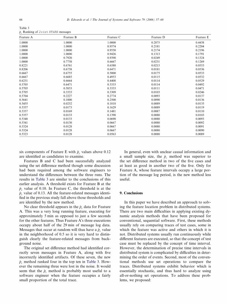
Table 3pc Ranking of Joint STARS messages

Feature A Feature B Feature C Feature D Feature E

1.0000 1.0000 1.0000 0.2875 0.44381.0000 1.0000 0.9574 0.2181 0.22041.0000 1.0000 0.9550 0.2174 0.21961.0000 1.0000 0.9426 0.1313 0.17911.0000 0.7920 0.9398 0.0249 0.13241.0000 0.7758 0.6667 0.0231 0.12690.8221 0.6761 0.6580 0.0215 0.05530.8206 0.6758 0.6471 0.0181 0.05360.6667 0.6755 0.5000 0.0175 0.05330.6667 0.6685 0.4953 0.0115 0.05320.6251 0.6664 0.4408 0.0114 0.05290.5705 0.6471 0.3333 0.0114 0.04920.5705 0.5853 0.3333 0.0111 0.04710.5705 0.3333 0.3309 0.0103 0.02460.5704 0.2227 0.2774 0.0093 0.01370.5641 0.1000 0.2500 0.0090 0.01360.5455 0.0252 0.1818 0.0089 0.01350.5357 0.0173 0.1629 0.0089 0.01190.5357 0.0169 0.1481 0.0087 0.01100.5357 0.0133 0.1390 0.0080 0.01030.5348 0.0133 0.0690 0.0080 0.00930.5341 0.0130 0.0667 0.0080 0.00920.5324 0.0128 0.0667 0.0080 0.00910.5324 0.0128 0.0667 0.0080 0.00900.5323 0.0128 0.0563 0.0080 0.0089


six components of Feature E with pc values above 0.12are identified as candidates to examine.

Features B and C had been successfully analyzedusing the set difference method though some discussionhad been required among the software engineers tounderstand the differences between the three runs. Theresults in Table 3 are similar to the conclusions of thisearlier analysis. A threshold exists for Feature B at thepc value of 0.10. In Feature C, the threshold is at thepc value of 0.13. All the feature-related messages identi-fied in the previous study fall above those thresholds andare identified by the new method.

No clear threshold appears in the pc data for FeatureA. This was a very long running feature, executing forapproximately 5 min as opposed to just a few secondsfor the other features. Thus Feature A�s three executionsoccupy about half of the 29 min of message log data.Messages that occur at random will thus have a pc valuein the neighborhood of 0.5 so it is very hard to distin-guish clearly the feature-related messages from back-ground noise.

The original set difference method had identified cor-rectly seven messages in Feature A, along with fiveincorrectly identified artifacts. Of these seven, the newpc method ranked four in the top ten in Table 3. How-ever the remaining three were lost in the noise. It wouldseem that the pc method is probably most useful to asoftware engineer when the feature occupies a fairlysmall proportion of the total trace.

In general, even with unclear causal information anda small sample size, the pc method was superior tothe set difference method in two of the five cases andat least as good in another two of the five. Only forFeature A, whose feature intervals occupy a large por-tion of the message log period, is the new method lessuseful.

9. Conclusions

In this paper we have described an approach to solv-ing the feature location problem in distributed systems.There are two main difficulties in applying existing dy-namic analysis methods that have been proposed forconventional, sequential software. First, these methodsusually rely on comparing traces of test cases, some inwhich the feature was active and others in which it isnot. Distributed systems usually run continuously whiledifferent features are executed, so that the concept of testcase must be replaced by the concept of time interval.However, the determination of precise time intervals indistributed system is complicated by difficulties in deter-mining the order of events. Second, most of the conven-tional methods use set operations to compare thetraces. Distributed systems exhibit behavior which isessentially stochastic, and thus hard to analyze usingall-or-nothing set operations. To address these prob-lems, we proposed:


(1) A definition of a time interval based on causal order-ing of events as described by Lamport and others.The time interval delimits events for mapping tosoftware components potentially associated withthe feature.

(2) A component relevance index, pc, that can be esti-mated to rank components. Accuracy level of theestimate improves by increasing the number of timeintervals.

(3) A weighting function, x( ), that is the means forcomputing pc. Different weighting functions can beused depending on the nature of the system beingstudied and on the precision of the available data.The value of x( ) is 1.0 for events causally includedin the interval, and decreases for events as their tem-poral proximity to the interval decreases. Temporaldistance from an interval to an event is measuredalong the shortest causal path.

Two case studies were presented. The basic propertiesof pc were explored in the first study where its estimatesquickly converged and clearly distinguished betweenfeature-related code and background noise. The methodworked well even when intervals were only approxi-mately delineated. The second study analyzed messagelogs from Joint STARS, a large-scale distributed system.Although intervals were imprecisely defined, messageswere effectively ranked to enabled the investigation ofseveral features. The ranking included two featureswhich could not be analyzed in an earlier study.

Our approach addresses the identified difficultiesencountered in the transition from sequential to distrib-uted systems. Incorporation of our method into analysisand debugging tools can provide insights to the softwareengineers for isolating relevant components. Our meth-od is straightforward to implement provided the systemcan tolerate logging of messages and events.

References

Agrawal, H., Alberi, J., Horgan, J., Li, J.J., London, S., Wong, W.E.,Ghosh, S., Wilde, N., 1998. Mining system tests to aid softwaremaintenance. IEEE Computer 31 (7), 64–73.

Anceaume, E., Helary, J.-M., Raynal, M., 2002. Tracking immediatepredecessors in distributed computations. In: Proceedings of theFourteenth Annual ACM Symposium on Parallel Algorithms andArchitectures. ACM Press, Winnipeg, Canada, pp. 210–219.

Arora, A., Kulkarni, S., Demirbas, M., 2000. Resettable vector clocks.In: Proceedings of the Nineteenth Annual ACM Symposium onPrinciples of Distributed Computing. ACM Press, Portland,Oregon, USA, pp. 269–278.

Biggerstaff, T., Mitbander, B., Webster, D., 1994. Program under-standing and the concept assignment problem. Communications ofthe ACM 37 (5), 72–83.

Chen, K., Rajlich, V., 2000. Case study of feature location usingdependence graph. In: Proceedings of the Eighth InternationalWorkshop on Program Comprehension––IWPC 2000. IEEEComputer Society, Los Alamitos, CA, pp. 241–249.

Cooper, R., Marzulo, K., 1991. Consistent detection of globalpredicates. In: Proceedings of the ACM SIGPLAN and SIGOPSWorkshop on Parallel and Distributed Debugging, pp. 163–173.

Deprez, J., Lakhotia, A., 2000. A formalism to automate mappingfrom program features to code. In: Proceedings of the EighthInternational Workshop on Program Comprehension––IWPC2000. IEEE Computer Society, Los Alamitos, CA, pp. 69–78.

Eisenbarth, T., Koschke, R., Simon, D., 2002. Incremental location ofcombined features for large-scale programs. In: Proceedings of theIEEE International Conference on Software Maintenance, Mon-treal, Canada, pp. 273–282.

Fidge, C., 1988. Timestamps in message-passing systems whichpreserve the partial ordering. In: Proceedings of the EleventhAustralian Computer Science Conference, pp. 56–66.

Garg, K.K., Chase, C., 1995. Distributed algorithms for detectingconjunctive predicates. In: International Conference of DistributedComputing Systems, pp. 423–430.

Koenemann, J., Robertson, S., 1991. Expert problem solving strategiesfor program comprehension. In: CHI�91 Conference Proceedings.Association for Computing Machinery, pp. 125–130.

Lamport, L., 1978. Time, clocks, and the ordering of events in adistributed system. Communications of the ACM 21 (7), 558–565.

Mattern, F., 1989. Virtual time and global states of distributedsystems. In: Cosnard et al. (Eds.), Proceedings of the InternationalWorkshop on Parallel and Distributed Algorithms. North-Holland, Amsterdam, pp. 215–226.

Message Passing Interface Forum, 1995. MPI: A message-passinginterface standard (version 1.1). Tech. rep., MPI-Forum. Availablefrom: <http://www.mpi-forum.org>.

Message Passing Interface Forum, 1997. MPI-2: Extensions to themessage-passing interface. Tech. rep., MPI-Forum. Availablefrom: <http://www.mpi-forum.org>.

Musa, J., 1998. Software Reliability Engineering. McGraw-Hill, NewYork.

Northrop Grumman, 2004. Joint surveillance target attack radarsystem (JSTARS). Available from: <http://www.capitol.north-grum.com/programs/jstars.html>.

Schutz, W., 1994. Fundamental issues in testing distributed real-timesystems. Real-Time Systems 7 (2), 129–157.

Sim, S.E., Clarke, C.L.A., Holt, R.C., 1998. Archetypal source codesearches: A survey of software developers and maintainers. In:Proceedings of the International Workshop on Program Com-prehension. IEEE Computer Society Press, Los Alamitos, CA,pp. 180–187.

Telecordia Technologies, Inc., 2003. XSUDS—telcordia softwarevisualization and analysis toolsuite. Available from: <http://xsuds.argreenhouse.com/>.

Weiser, M., 1982. Programmers use slices when debugging. Commu-nications of the ACM 25 (7), 446–452.

Wilde, N., May 2003. RECON2––tool for C programmers. Availablefrom: <http://www.cs.uwf.edu/~recon/>.

Wilde, N., Buckellew, M., Page, H., Rajlich, V., 2001. A case study offeature location in unstructured legacy Fortran code. In: Proceed-ings of the Fifth European Conference on Software Maintenanceand Reengineering—CSMR�01. IEEE Computer Society, Lisbon,Portugal, pp. 68–76.

Wilde, N., Casey, C., 1996. Early field experience with the softwarereconnaissance technique for program comprehension. In: Pro-ceedings of the IEEE International Conference on SoftwareMaintenance, Monterey, California, pp. 312–318.

Wilde, N., Casey, C., Vandeville, J., Trio, G., Hotz, D., 1998. Reverseengineering of software threads: A design recovery technique forlarge multi-process systems. Journal of Systems and Software 43,11–17.

Wilde, N., Scully, M., 1995. Software reconnaissance: Mappingprogram features to code. Journal of Software Maintenance:Research and Practice 7, 49–62.

http://www.mpi-forum.org

http://www.mpi-forum.org

http://www.capitol.northgrum.com/programs/jstars.html

http://www.capitol.northgrum.com/programs/jstars.html

http://xsuds.argreenhouse.com/

http://xsuds.argreenhouse.com/

http://www.cs.uwf.edu/~recon/


Wong, W.E., Gokhale, S.S., Horgan, J.R., 1999a. Metrics forquantifying the disparity, concentration, and dedication betweenprogram components and features. In: Sixth IEEE InternationalSymposium on Software Metrics, p. 189.

Wong, W.E., Horgan, J.R., Gokhale, S.S., Trivedi, K.S., 1999b.Locating program features using execution slices. In: 1999 IEEESymposium on Application-Specific Systems and Software Engi-neering and Technology, p. 194.

Documents

An approach to feature location in distributed systems