Embed Size (px)
Citation preview

AN Approach to stimulation candidate selection
and optimization
A
Research Thesis
Presented to the Department of Petroleum Engineering,
African University of Science and Technology,
Abuja
in Partial Fulfillment of the Requirements for the Award of Master of
Science (MSc)
in
Petroleum Engineering
By
BENSON OGHENOVO UGBENYEN
Abuja, Nigeria November, 2010

An Approach to Stimulation Candidate Selection and Optimization
By
Benson Oghenovo Ugbenyen
RECOMMENDED: ________________________________
________________________________
________________________________
________________________________
APPROVED: ________________________________ Supervisor: Prof. (Emeritus) David O. Ogbe
________________________________
________________________________
________________________________
Date
iii | An Approach to Stimulation Candidate Selection and Optimization
ABSTRACT
Well stimulation consists of several methods used for enhancing the natural producing ability of
the r eservoir when p roduction rate declines. A de tailed l iterature r eview of s ome of t he well
published stimulation models are discussed in this research. This d iscussion wa s preceded wi th
an introduction t o f ormation damage concepts and an o verview o f well stimulation m ethods.
Production decline curve analysis is combined with economic discounting concepts to develop a
model that can be used for optimizing stimulation decisions. The model is presented in the form
of a no n-linear programming pr oblem subject t o t he constraints imposed by t he p roduction
facilities, reservoir productivity and the stimulation budget approved by management. Production
data from four stimulation candidate wells, o ffshore Niger Delta was used to validate the model
developed by s etting up a maximization problem. Solution to the p roblem was ob tained using
non-linear o ptimization software. The r esult o btained was v erified u sing Wolfram R esearch’s
Mathematica 7.0. The results s how that the o ptimization m odel c an be c ombined w ith
stimulation t reatment modules, de veloped f rom i ndustry w ide models, t o q uantify s timulation
benefits. C andidate w ells w ere t hen r anked ba sed on stimulation c ost, p ayout t ime a nd
stimulation b enefit. Hence, th e m odel i s valid f or stimulation ca ndidate s election; and i s
therefore recommended for use in optimizing stimulation decisions.

iv | An Approach to Stimulation Candidate Selection and Optimization
DEDICATION
This research is dedicated to my Lord Jesus Christ who has been, and will ever be the best role
model anyone could find. And also, to the good people of the Niger Delta.

v | An Approach to Stimulation Candidate Selection and Optimization
ACKNOWLEDGEMENT I wish t o sincerely a ppreciate G od Almighty for H is l ove, c are a nd wonderful works t hat a re made m anifest i n m y life each da y. Also, m y s incere thanks go to my supervisor, Prof. (Emeritus) David O. Ogbe for guiding me to success in this work, Dr. Samuel Osisanya and Prof. Peters Ekwere f or s erving in m y thesis committee, and m y m other, M rs. G race Ugbenyen f or being there always for me. The following persons, among others, who contributed in no small measure to the success of this work deserved to be acknowledged. My friends: Lymmy B ukie O gbidi, Akpana Paul, R aymond Agav, Habibatu Ahmed, and Christopher Mudi who paid m e several v isits a t A UST t o c heer me u p. T he members o f H ope Hall Parish, Redeemed Christian Church of God, Galadimawa, Abuja, who have always been a warm family to me. Nature will not forgive me if I fail to thank Miss Esther Akinyede who was kind to provide me with a laptop to continue this work when lightning storm damaged my laptop on 14th
July 2010 a t Julius Nyerere Hall, AUST, Abuja, and I got no help from the University even t hough I pl eaded f or assistance. I w ill n ot f ail to m ention Mr. Alfred Emakpose who assisted me in no small measure to keep things straight when the odds were against me. Finally, I would like to thank my wonderful new friends, who would be mad at me if I fail to mention their names; Hatem, Adel, Amar, Fauzan and Andrew, who are here with me as I write these lines at The Beaches Hotel, Prestatyn, North Wales, where I neglected some of my schedule to put most parts of this work together.

vi | An Approach to Stimulation Candidate Selection and Optimization
TABLE OF CONTENTS
ABSTRACT……………………………………….………….....iii
DEDICATION…………………………………….…………....iv
ACKNOWLEDGEMENT…………………………….………...v
TABLE OF CONTENT………………………………………...vi
LIST OF FIGURES……………………………….………….....x
LIST OF TABLES………………………………………………xi
CHAPTER ONE: INTRODUCTION 1.1 The Near Wellbore Condition…………………………………….……………….…....1
1.1.1 The Composite Skin Effect…………………………………………….…….....1
1.2 Well Stimulation: Definition and Objectives………………………………….….……..1
1.2.1 Well Stimulation Objectives………………………………………………….…1
1.3 Well Stimulation Methods…………………………………………………….………...2
1.3.1 Matrix Stimulation……………………………………………………………....2
1.3.1.1 Matrix Acidizing Fluid Selection and Treatment Additives ……………....3
1.3.1.2 Benefits and Limitations of Matrix Acidizing Processes………………......4
1.3.2 Fracture Acidizing…………………………………………………….…….......4
1.3.3 Hydraulic Fracturing…………………………………………………….……....6
1.3.4 Recompletion……………………………………………………………….…...7
1.4 Gravel Packing………………………………………...……………………………...…7
1.5 Stimulation Economics and Candidate Selection……………………………….……....8
1.6 Objective and Procedure of the Study…………..………………………………………8
1.7 Limitation of the Study……………………..………………………………………...…9
CHAPTER TWO: LITERATURE REVIEW 2.1 Review of Formation Damage Mechanism…………………………………….….........10
2.1.1 Definition…………………………………………………………….……….…10
2.1.2 Causes of Formation Damage……………………………………………….….10
2.1.3 Quantifying Formation Damage………………………………………..……….11
2.1.3.1 Skin Factor……………………………………………………….……...…11

vii | An Approach to Stimulation Candidate Selection and Optimization
2.1.3.2 Depth of Damage……………………………………………………….…13
2.1.3.3 Damage Ratio………………………………………………………….…..14
2.1.3.4 Flow Efficiency…………………………………………………………....16
2.1.3.5 Permeability Variation Index………………………………………….…..16
2.1.4 Economic Impact of Formation Damage on Reservoir Productivity
………………………...…………….….17
2.2 Matrix Acidizing Models………………………………………………..………….…..17
2.2.1 Sandstone Acidizing Models……………………………………………….…..18
2.2.2 Carbonate Acidizing Models……………………………………………….…..22
2.3 Acid Fracturing Models……………………………………………………………..….26
2.4 Hydraulic Fracturing Models……………………………………………..……….……28
2.5 Literatures on Stimulation candidate Selection…………………………………….…...30
CHAPTER THREE: METHODOLOGY 3.1 Well Screening Technique……………………………………………..…………….…33
3.2 Design of Stimulation Treatment Models………………………………………….…...34
3.2.1 Matrix Acidizing Design Model…………………….……………………….…38
3.2.1.1 Summary……………………………………………………………….….38
3.2.2 Recompletion Design Model……………………………………………….…..38
3.2.3 Gravel-Pack Design Model……………………………………………….….…40
3.3 Development of a Model for Optimizing Stimulation Decisions………………….…..44
3.3.1 Optimization Model Assumptions…………………………………………..….45
3.3.2 Stimulation Productivity Ratio…………………………………………….…...46
3.3.3 The Present-value Discount Factor……………………….……………….…....46
3.3.4 Defining the Objective Function, QD
3.4 Optimization Model Constraints…………………………...……….…………….……50
…………………………………….…….46
3.4.1 Constraint 1: Break-even Requirement……………………...…………….……51
3.4.2 Constraint 2: Remaining Reserve Limitation…………………………….…….51
3.4.3 Constraint 3: Flow String capacity……………………………………….…….52
3.4.4 Constraint 4: Budget Allocation………………………………………….…….53
3.4.5 Constraint 5: Maximum Formation Productivity ratio……...…………….……53
3.4.6 Constraint 6: Productivity Improvement………………………………….……54
viii | An Approach to Stimulation Candidate Selection and Optimization
3.5 Stimulation Cost and Productivity Ratio Relationship………………………….……..54
3.6 Summary of the Optimization Model………………………………….………….……55
3.7 Solution to the Optimization Model………………………………………………..…..56
CHAPTER FOUR: MODEL VALIDATION, RESULTS AND DISCUSSION 4.1 Sensitivity Analysis…………………………………………………...…………….….58
4.1.1 Effect of Price of Oil…………………………………………….……………...58
4.1.2 Effect of Discount Rate……………………………………………….…….….58
4.1.3 Effect of Decline Rate……………………………………………………….…58
4.1.4 Effect of Pre-Stimulation Production rate…………………......………….........63
4.1.5 Effect of Abandonment Rate……………..……………………………………63
4.1.6 Effect of Stimulation Time……………………………………………….…….66
4.2 Model Validation: Case Study 1 ……………………...……………………….….…...66
4.2.1 Formulation of the Bestfield Model…………………………………….……....66
4.2.2 Solution of the Well BU 3 Model…………………………………………..…...72
4.2.3 Discussion of the Well BU 3 Model Result……………………………….……73
4.2.4 Application of the Model Result in Candidate Selection…………………..…..74
4.2.5 Effect of Price of Oil on Well BU 3 Model Result……………………….…….74
4.3 Model Validation: Case Study 2………………………………………………….……77
4.3.1 Formulation of Well BU 5 Model……………………………………….……...77
4.3.2 Solution of the Well BU 5 Model……………………………………….………80
4.3.3 Discussion of the Well BU 5 Model Result…….………………………..……...81
4.3.4 Effect of Oil Price on Well BU 5 Model Result………………………………...82
4.3.5 Using Case Study 2 Model Result in Candidate Selection……………..………82
CHAPTER FIVE: CONCLUSION AND RECOMMENDATION
5.1 Conclusion…………………………………………………………………………...…84
5.2 Recommendation…………………………………………………………………….…85
REFERENCES…………………………………………………………………………….…….87
NOMENCLATURE………………………………………………………………………….….95
APPENDIX A: A SIMPLE WELL SCREENING FLOW CHART…………………………...98

ix | An Approach to Stimulation Candidate Selection and Optimization
APPENDIX B: STIMULATION COST AND PERFORMANCE………………………….....99
APPENDIX C: SOLVER RESULTS………………………………………………………….100
APPENDIX D: WHAT’S BEST 10.0 RESULTS……………………………………………...115
APPENDIX E: MATHEMATICA 7.0 RESULTS……………………………………………..120
APPENDIX F: DERIVATION OF THE OBJECTIVE FUNCTION FOR OTHER
DECLINE CASES……………………………………………………….…..124
x | An Approach to Stimulation Candidate Selection and Optimization
LIST OF FIGURES
3.1 Production Decline Profile for a Stimulated Well.………………… ……………….…45
4.1 Effect of oil price on the objective function ………….…………………………….….60
4.2 Effect of discount rate on the objective function …………………..……………….….61
4.3 Effect of decline rate on the objective function ……………………………………..…62
4.4 Effect of pre-stimulation production rate on the objective function……………….…...64
4.5 Effect of abandonment rate on the objective function ………………...………….........65
4.6 Effect of stimulation time……………………………………….………………….…...67
4.7 Cost Versus Productivity Ratio Plot for Well BU 3…..……………………………...…71
4.8 Effect of oil price on Well BU 3 model result……………………………………….…..76
4.9 Cost Versus Productivity Ratio Plot for Well BU 5 ……………………………….……79
4.10 Effect of oil price on Well BU5 model result………………………………………….83

xi | An Approach to Stimulation Candidate Selection and Optimization
LIST OF TABLES
Table 4.1: Input Data for Sensitivity Analysis…………….………..59
Table 4.2: Bestfield Model Data……………………………….…….68
Table 4.3: Bestfield Model Summary………………………………..75
Table 4.4: Well BU 5 Model Data…………………………………...78

1 | An Approach to Stimulation Candidate Selection and Optimization
Chapter One
Introduction
1.1 The Near Wellbore Condition
Permeability reduction i n t he r egion near t he wellbore in a producing zo ne i s r eferred t o a s
“damage”. The damaged region i s c alled s kin z one w hile the term “skin e ffect” refers t o a
dimensionless parameter used to quantify the extent of damage. Reduction in permeability in the
near-wellbore region results in lower productivity due to increased pressure drop, hence damage
is not desirable.
1.1.1 The Composite Skin Effect
The skin effect can be o btained from a well te st. I t measures t he extent of damage in t he near-
wellbore zone. The total skin effect obtained from the well test is a composite parameter which
consists of s kin c omponents d ue to mechanical c auses – a di sturbance of t he fluid f low
streamline n ormal t o t he w ell, o r formation damage - alteration o f t he natural r eservoir
permeability. It is very important to be able to identify the formation damage component of the
skin s ince t his c an b e r educed by b etter operational practices, or possibly, b e r emoved or
bypassed by stimulation treatments. Formation damage can result from many different operations
such a s dr illing, cementing, perforating, completion/gravel pa cking, production, i njection,
workover, stimulation, etc.
1.2 Well Stimulation: Definition and Objectives
Well stimulation is a way of increasing well productivity by removing (or bypassing) formation
damage in t he near-wellbore r egion or by superimposing a highly conductive structure onto the
formation.
1.2.1 Well Stimulation Objectives
The objectives of w ell s timulation can be di vided into technical ob jectives and e conomic
objectives.
2 | An Approach to Stimulation Candidate Selection and Optimization
• Technical Objectives
Remove, reduce or b ypass t he f ormation damage, reduce sand production and cl eaning-
up the perforations.
• Economic Objectives
Increase flow rate and optimize production from the reservoir.
1.3 Well Stimulation Methods
Several stimulation t echniques e xist bu t t he commonly u sed methods i nclude matrix a cidizing,
fracture a cidizing, fracpack, ex treme o verbalance operations and hy draulic fracturing. These
methods h elp t o optimally increase well or reservoir productive c apacity by providing a net
increase in the productivity index. This increase in productivity index can then be used either to
increase t he p roduction r ate o r t o d ecrease the dr awdown pressure differential. Increase i n
production rate will eventually increase productivity. A decrease in drawdown can help prevent
sand pr oduction and water or gas coning and/or shift the phase equilibrium in the near-wellbore
region t owards s maller f ractions of condensate. Some of the m ost c ommon s timulation
techniques are discussed in the following sections.
1.3.1 Matrix Stimulation
Matrix stimulation is injecting an acid/solvent into the formation at below the fracturing pressure
of t he formation to d issolve/disperse materials th at im pair well production i n sandstone
reservoirs or to create new, unimpaired flow channels in carbonate reservoirs. Mineral acids are
most c ommonly us ed in matrix s timulation hence t his t echnique is f requently ca lled ma trix
acidizing. Matrix acidizing is a near-wellbore treatment, with all of the acid reacting within a few
to perhaps as much as 10 ft of the wellbore in carbonates. Matrix a cidizing lower permeability
limit is 10mD for oil wells and 1mD for gas wells.
In sandstone, only a small f raction o f the m atrix i s soluble hence r elatively s low r eacting acid
dissolves the permeability-damaging minerals. Carbonate formations are different in that a large
fraction of the matrix is soluble (usually > 50%), hence acid will react rapidly with flow channels
and pores and creates new flow paths by dissolving the formation rock.

3 | An Approach to Stimulation Candidate Selection and Optimization
As a rule of thumb, matrix acidizing i s a pplied only in situations where a well has a large skin
effect t hat cannot b e attributed t o mechanical, o peration o r surface p roblems. The r emoval of
damage by matrix a cidizing r equires t hat t he t ype ( or c ause) a nd location of t he damage be
identified before its removal is attempted. The damage identification process involves:
• Examining t he well r ecords to i dentify operations t hat might ha ve r esulted in formation
damage
• Carrying out specific laboratory testing, such as a reservoir core flushing, to determine if
the identified operations did indeed lead to core damage for the particular combination of
the fluids in question and the reservoir formation
• Examining t he da maged core with sophisticated a nalytical techniques s uch a s t he
scanning electron microscope to confirm the damage type and the damage location and
hence develop ideas on how to remove it.
1.3.1.1. Matrix Acidizing Fluid Selection and Treatment Additives
The t ype of a cid u sed for a s timulation j ob i s a function of t he da mage t ype. Generally, a cid
selection guidelines are based on temperature, mineralogy and petrophysics. The most common
acids u sed a re h ydrochloric a cid ( HCl) a nd a m ixture o f hydrochloric a nd h ydrofluoric a cids
(HF/HCl) usually known a s mud acid. HCl is suitable f or li mestone, d olomite, formation w ith
iron m aterials a nd C aSO4
Additives help make acid treatments more e ffective. They are mixed with the treating fluids to
modify a pr operty of t he fluid (e.g., corrosion, p recipitation, emulsification, s ludging, s caling, f ines
migration, clay swelling tendency, surface tension, flow per layer, friction pressure). The treating fluid
is d esigned t o e ffectively r emove or b ypass t he damage, whereas a dditives a re u sed t o prevent
excessive c orrosion, p revent s ludging and e mulsions, pr event iron pr ecipitation, improve
cleanup, improve coverage of the zone and pr event pr ecipitation of reaction products. Additives
. H F i s mostly us ed i n s andstone, c lay, f eldspar, s and (spent on
material, not quartz or sand), and it is not used in carbonate formations. Acid mixtures such as
acetic-hydrochloric a nd formic-hydrochloric a cids a re u sed i n high temperature ca rbonate
formation w hile t he formic-hydrofluoric a cid mixture i s us eful i n high t emperature sandstone
formation.
4 | An Approach to Stimulation Candidate Selection and Optimization
are a lso u sed i n preflushes a nd overflushes t o stabilize clays a nd di sperse pa raffins a nd
asphaltenes. Types of additives include: acid corrosion inhibitors, aromatic solvents, Iron stabilizers,
surfactants, mutual solvents, diverters, scale i nhibitors, clay stabilizers, aluminum stabilizer, retarders,
nitrogen and alcohols.
1.3.1.2. Benefits and Limitations of Matrix Acidizing Processes
Matrix a cidizing is usually very economically a ttractive (low c ost), because r elatively s mall
treatments may improve the well performance considerably.
Some pr oblems a ssociated with matrix a cidizing a re: difficulty to i dentify the type of damage,
multiple damages with completing remedies, detrimental by-products o f stimulation, frequently,
ineffective o r p artially e ffective treatments. It involves complex chemical a nd t ransport
phenomena t hat, w hile effective i n r emoving one k ind o f damage, may cr eate a nother o ne.
HCL/HF blends can create early damage in formations, however the lower the HF concentration
in t he b lend t he l ess chance there i s for damage creation. Acid placement and damage removal
from l aminated f ormations w here some perforations penetrate very h igh-permeability la yers is
especially problematic.
Successful m atrix treatments r equire correct c hoice of fluid t o a ttack damage an d u niform
placement o f the s elected treating f luid. Improper f luid pl acement i ncreases reservoir
heterogeneity. Misapplied stimulation treatments a re costly and ineffective, o ften creating more
problems than they solve.
It is important to note that not all da mage can be removed by matrix acidizing. Whenever there
are insoluble scales (e.g. BaSO4) or acid s ensitive sandstones, other s timulation methods (such
as acid fracturing to bypass scales) are considered.
1.3.2 Fracture Acidizing
In this method of acidizing, acid is injected into the formation at a rate high enough to generate
the pressure required t o fracture t he formation. T he r apid i njection produces a buildup i n the

5 | An Approach to Stimulation Candidate Selection and Optimization
wellbore pressure until it is large enough to overcome compressive earth stresses and the rock’s
tensile strength. At this p ressure, t he r ock fails, a llowing a c rack ( fracture) t o be formed.
Continued fluid injection increases the fracture length and width. The injected acid differentially
etches t he formation fracture faces as it r eacts, r esulting i n t he formation of h ighly c onductive
etched channels that remain open after the fracture closes. Two procedures are commonly used.
Acid alone i s injected, or a fluid ( called a pad) that will create a long, wide fracture is injected
and followed by an a cid. A conventional fracture acidizing treatment involves pumping an acid
system after fracturing. It may be preceded by a nonacid preflush and usually is overflushed with
a nonacid fluid.
Acid s olubility of th e f ormation is a key f actor i nfluencing w hether f racture acidizing or
proppant treatments should be employed. If the formation is less than 75% acid soluble, proppant
treatments should be used. For acid solubilities between 75 and 85%, special lab work can help
define w hich approach should be used. Above 85% acid solubility, fracture acidizing would b e
the most effective approach.
Treatment v olumes for fracture a cidizing a re much l arger t han for matrix acidizing t reatments,
being as high as 1,000 to 2,000 gal/ft of perforated interval.
As a general guideline, f racture a cidizing i s us ed on formations with > 80% hydrochloric a cid
solubility. Low-permeability carbonates (>20 md) a re t he best candidates for t hese t reatments.
Fluid loss to the matrix and natural fractures can also be better controlled in lower permeability
formations.
The su ccess of t he acid f racturing treatment depends on two ch aracteristics o f t he etched
fracture: effective fracture length (which is a function of the rate of acid consumption, acid fluid
loss ( wormhole formation) a nd acid convection a long t he fracture) a nd e ffective fracture
conductivity (a function of the etched pattern, vo lume of r ock di ssolved, r oughness of etched
surface, rock strength and closure st ress). The acidized fracture length and fracture conductivity
are therefore controlled largely by the treatment design and formation strength.
6 | An Approach to Stimulation Candidate Selection and Optimization
1.3.3 Hydraulic Fracturing
Hydraulic Fracturing consists of pumping a viscous fluid at a sufficiently high pressure (greater
than the formation fracture pressure) into the completion interval so that a two winged, hydraulic
fracture is formed. This fracture is then filled with a high conductivity, proppant which holds the
fracture open (maintains a high conductivity path to the wellbore) after the treatment is finished.
Propped hydraulic fracturing is aimed at raising the well productivity by increasing the e ffective
wellbore radius f or w ells c ompleted i n low p ermeability c arbonate or clastic f ormations.
Hydraulic fracturing i s t o improve productivity i n l ow-permeability f ormations, or to pe netrate
near-wellbore damage or for sand control in higher permeability formations.
Hydraulic fracturing is a mechanical process hence it is only necessary to know that formation
damage is present when designing such a treatment. When a well is hydraulically fractured, most
pre-treatment skin e ffects such a s f ormation da mage, perforation skins a nd s kins d ue t o
completion and partial penetrations are bypassed and have no effect on the post-treatment w ell
performance. Phase-and r ate-dependent skins effects a re either eliminated or contributes i n the
calculation of the fracture skin effects. Generally pre-treatment skin effects are not added to post-
fracture skin effects.
Hydraulic fracturing differs from fracture acidizing in that hydraulic fracturing fluids usually are
not c hemically r eactive, a nd a pr oppant i s placed i n the f racture t o keep the f racture open and
provide conductivity.
The Inflow Performance of a Fracture Stimulated well i s controlled by a quantity known as t he
dimensionless fracture conductivity which depends on the fracture permeability conductive
fracture w idth, f ormation permeability and the conductive fracture single wing length. The
fracture c onductivity i s i ncreased by an i ncreased fracture width, a n i ncreased proppant
permeability ( large, more spherical p roppant grains ha ve higher permeability), a nd m inimizing
the permeability damage to the proppant pack from the fracturing fluid.
Propped hy draulic f racture w ell s timulation s hould onl y be c onsidered when the: well i s
connected to adequate produceable reserves; reservoir pressure is h igh enough to maintain flow
7 | An Approach to Stimulation Candidate Selection and Optimization
when producing t hese r eserves ( or i t i s economically ju stifiable to i nstall a rtificial li ft);
production s ystem can pr ocess t he e xtra pr oduction; professional, experienced p ersonnel are
available for t reatment de sign, e xecution a nd supervision t ogether with h igh quality pu mping,
mixing and blending equipment.
1.3.4 Recompletion
For wells with certain t ypes of da mage such a s pa rtially or t otally p lugged p erforations,
insufficient perforation density o r low depth of perforation, it may b e sufficient t o r ecommend
recompletion technique. Hence the idea of recompletion is to increase the perforation density or
to increase the depth of perforations. The overall aim of this method is to increase production by
bypassing t he da mage. R ecompletion i s a lso u sed effectively in reducing water p roduction. I n
this approach t he w ell i s re-perforated at a new hi gher z one w hile t he pe rforations i n t he wa ter
zone are plugged off.
1.4 Gravel Packing
Gravel packing is used in weak formations that have been producing sand or have the tendency
of producing s and. The gr avel m ixed in a ba se f luid is pu mped as sl urry to f ill all p erforation
tunnels and t he s creen/casing a nnulus. Productivity a nd l ife of t he gravel pack depends on
packing t he perforations w ith gr avel. If not pa cked, f ormation f ines c an invade t he tunnels
impairing productivity and also reducing the area open to flow. Re-completions in low pressure
reservoirs w here formation s and ha s be en pr oduced, can accept l arge volumes o f additional
gravel.
1.5 Stimulation Economics and Candidate Selection
The evaluation of the economics of stimulation treatment must consider many factors including:
treatment cost, initial increase in production rate, additional reserve that may be produced before
the well reaches i ts economic l imit, rate of pr oduction d ecline b efore and a fter s timulation, and
reservoir and mechanical problems that could cause the treatment to be unsuccessful.
Selection of the optimum size of a stimulation treatment is based primarily on economics. The
most c ommonly used m easure of e conomic e ffectiveness is t he n et present v alue (NPV). The

8 | An Approach to Stimulation Candidate Selection and Optimization
NPV is the difference between the present value of all receipts and costs, both current and future,
generated a s a r esult of t he stimulation treatment. Future r eceipts and costs a re converted i nto
present va lue u sing a discount rate and taking i nto a ccount the year in which t hey will a ppear.
Another measure of t he economic e ffectiveness i s t he payout period (PO); t hat is, t he t ime i t
takes for the cumulative present value of the net well revenue to equal the treatment costs. Other
indicators i nclude i nternal rate of return (IRR), profit-to-investment ratio (PIR) and gr owth rate
of return (GRR). The NPV (as well as other indicators) is sensitive to the discount rate and to the
predicted future hydrocarbon pr ices. A s with a lmost a ny other e ngineering a ctivities, costs
increase almost linearly with the size of the stimulation tr eatment but (after a certain point) the
revenues increase only marginally or may even decrease. This suggests that there is an optimum
size of t he t reatment t hat will maximize t he N PV. Hence it i s i mportant to select stimulation
candidate wells that have potentials for maximum benefit.
Candidate Selection (Recognition) is the process of identifying and selecting wells for treatment
which have the capacity for higher production and better economic return. Hence in stimulation
candidate w ell s election, t he w ell s timulation treatment yielding the hi ghest di scounted rate o f
return is the treatment which, in principle, should be carried out first.
1.6 Objective and Procedure of the Study
The goal o f t his r esearch i s to present a model for i dentifying s timulation candidates,
recommending stimulation treatment option and optimizing the stimulation process selected. The
model i s a lso used to rank stimulation candidates ba sed on economics. Hence this research will
attempt to answer the question: “given the need to stimulate several wells in a field, how do we
rank the wells ba sed on s timulation benefit and what stimulation approach to use in or der to get
the highest economic returns?” To answer these questions, a merit function is developed based
on production decline curve analysis and economic discounting concepts. In combination with a
good stimulation treatment module, the model can be used for ranking stimulation candidates.
The research procedure begins i n chapter one with an introduction to the concept o f skin factor
and w ell s timulation methods. S everal lit eratures o n f ormation da mage a nd s timulation models

9 | An Approach to Stimulation Candidate Selection and Optimization
are r eviewed in chapter t wo. Chapter t hree c ontains a w ell s creening m odule, design o f s ome
selected stimulation modules and an optimization model which consists of an objective function
with constraint. The optimization model combines the concept of production decline curves with
economic d iscounting. The m odel de veloped i n chapter three is va lidated in chapter f our using
actual field data from the Niger Delta.
1.7 Limitation of the Study
This research is intended for stimulation candidate selection in the Niger Delta. Matrix acidizing
technique is the main stimulation technique that has been used up to date in the Niger Delta due
to t he g ood permeability of t he N iger D elta formation. Hence only matrix a cidizing t echnique,
recompletion and gravel packing are considered in the methodology presented in chapter three of
this research. Acid fracturing and hydraulic fracturing are not considered.
10 | An Approach to Stimulation Candidate Selection and Optimization
Chapter Two
Literature Review
In or der t o properly select s timulation candidate w ells, i t i s n ecessary t o first ha ve a n i n-depth
understanding of t he c oncepts of f ormation d amage and w ell s timulation. A lot of researches
conducted on formation da mage and well s timulation methods can be found in literatures. We ll
stimulation i s c onsidered a m ajor ke y t o proper r eservoir m anagement, he nce several a uthors
made valid contributions.
2.1 Review of Formation Damage Mechanism
2.1.1 Definition Civan1 defined formation d amage a s a g eneric t erminology r eferring t o t he i mpairment o f t he
permeability of petroleum bearing formations by various adverse processes. It is an undesirable
operational a nd e conomic problem t hat c an o ccur du ring t he va rious p hases of oi l a nd ga s
recovery f rom s ubsurface r eservoirs including d rilling, production, hydraulic f racturing, and
workover operations. Bennion2 viewed formation damage as any process that causes a reduction
in t he natural inherent pr oductivity of an o il and ga s pr oducing formation, or a reduction i n the
injectivity o f a water or gas in jection well. Bennion also pointed out that the formation damage
issue is often overlooked because of ignorance and apathy. In many cases, the operators are not
seriously c oncerned w ith f ormation d amage because of t he b elief t hat i t can be circumvented
later o n, simply b y a cidizing a nd/or h ydraulic fracturing. B ut Porter3 and M ungan4
argued t hat
because formation damage is usually nonreversible, it is better to avoid formation damage rather
than deal with it later on using expensive and complicated procedures.
2.1.2 Causes of Formation Damage Amaefule et al.5
classified the various factors causing formation damage as following:
• Invasion of f oreign f luids, s uch as w ater and c hemicals used for i mproved
recovery, drilling mud invasion, and workover fluids;
11 | An Approach to Stimulation Candidate Selection and Optimization
• Invasion o f foreign particles and mobilization of indigenous particles, such a s
sand, mud fines, bacteria, and debris;
• Operation conditions s uch a s w ell flow r ates a nd wellbore pr essures a nd
temperatures;
• Properties of the formation fluids and porous matrix.
Amaefule et al.5
further grouped these factors in two categories:
• Alteration of formation properties by various processes, including permeability reduction,
wettability a lteration, lithology c hange, r elease of mineral p articles, pr ecipitation of
reaction-by products, and organic and inorganic scales formation
• Alteration of fluid properties by various processes, including viscosity alteration by
emulsion block and effective mobility change.
2.1.3 Quantifying Formation Damage Terms used in quantifying formation damage as presented by various authors include:
2.1.3.1
Van Everdingen and Hurst
Skin Factor 6 defined skin effect or skin factor as a mathematically dimensionless
number which r eflects t he altered permeability d ue to damage 𝑘𝑘𝑑𝑑 , at a d istance rd, causing a
steady-state pressure difference. A relationship between the skin effect, s, reduced permeability,
𝑘𝑘𝑑𝑑 R and altered zone radius, rd
may be expressed as:
𝑠𝑠 = � 𝑘𝑘𝑘𝑘𝑑𝑑− 1� 𝑙𝑙𝑙𝑙 �𝑟𝑟𝑑𝑑
𝑟𝑟𝑤𝑤� ……………………………………….....…….2.1
Equation 2.1 is known as Hawkins7
formula. From the equation i t can be deduced that If 𝑘𝑘𝑑𝑑 <
𝑘𝑘 the well is damaged and 𝑠𝑠 > 0; conversely, if 𝑘𝑘𝑑𝑑 > 𝑘𝑘, then 𝑠𝑠 < 0 and the well is stimulated. For 𝑠𝑠 = 0,
the near-wellbore permeability is equal to the original reservoir permeability.
Generally, certain well logs may enable calculation of the damaged radius, rd , whereas pressure
transient analysis may provide the skin effect, s, and reservoir permeability, k. Equation 2.1 may
then be used to calculate the value of the altered permeability 𝑘𝑘𝑑𝑑 .

12 | An Approach to Stimulation Candidate Selection and Optimization
In the absence of production log data, Frick and Economides8
postulated that, an elliptical cone
is a more plausible shape of damage distribution along a horizontal well. They developed a skin
effect expression, analogous to the Hawkins formula:
𝑠𝑠𝑒𝑒𝑒𝑒 = � 𝑘𝑘𝑘𝑘𝑑𝑑− 1� 𝑙𝑙𝑙𝑙 � 1
𝐼𝐼𝑎𝑎𝑙𝑙𝑎𝑎 +1��4
3�𝑎𝑎𝑆𝑆𝑆𝑆 ,𝑚𝑚𝑎𝑎𝑚𝑚
2
𝑟𝑟𝑤𝑤2+ 𝑎𝑎𝑆𝑆𝑆𝑆 ,𝑚𝑚𝑎𝑎𝑚𝑚
𝑟𝑟𝑤𝑤+ 1� …….….…..2.2
where 𝑠𝑠𝑒𝑒𝑒𝑒 is the equivalent skin effect, 𝐼𝐼𝑎𝑎𝑙𝑙𝑎𝑎 is t he i ndex of a nisotropy a nd 𝑎𝑎𝑆𝑆𝑆𝑆 ,𝑚𝑚𝑎𝑎𝑚𝑚 is the
horizontal axis of the maximum ellipse, normal to the well trajectory. The maximum penetration
of d amage is n ear t he vertical section of t he well. T hey stated t hat the shape of t he el liptical
cross-section will depend greatly on t he i ndex of a nisotropy. The i ndex of anisotropy 𝐼𝐼𝑎𝑎𝑙𝑙𝑎𝑎 is
defined as:
𝐼𝐼𝑎𝑎𝑙𝑙𝑎𝑎 = �𝐾𝐾𝑆𝑆𝐾𝐾𝑉𝑉
……………………………………………….……..2.3
with 𝐾𝐾𝑆𝑆 being the horizontal permeability and 𝐾𝐾𝑉𝑉 is the vertical permeability.
Piot and Lietard9 expressed the total skin of a well as a sum of the pseudoskin of flow lines from
the f ormation face to t he pi peline and the true skin du e to f ormation da mage. Economides and
Nolte10
The total skin effect may be written as:
shown t hat t he t otal skin effect i s a composite of a number of factors, most of which
usually cannot be altered by conventional matrix treatments.
𝑠𝑠𝑡𝑡 = 𝑠𝑠𝑐𝑐+𝜃𝜃 + 𝑠𝑠𝑝𝑝 + 𝑠𝑠𝑑𝑑 + ∑𝑝𝑝𝑠𝑠𝑒𝑒𝑝𝑝𝑑𝑑𝑝𝑝𝑠𝑠𝑘𝑘𝑎𝑎𝑙𝑙𝑠𝑠 …………………...............2.4
The last term in the right-hand side of Eq. 2.3 represents an array of pseudoskin factors, such as
phase-dependent a nd r ate-dependent e ffects that c ould b e altered b y hy draulic f racturing
treatments. The other three terms are the common skin factors. The th ird term 𝑠𝑠𝑑𝑑 refers to the
damage skin e ffect as defined in equation 2.1. The fi rst term 𝑠𝑠𝑐𝑐+𝜃𝜃 is the skin effect caused by
partial completion and slant. Cinco-Ley et al.11 documented a detailed approach of estimating the
skin f actor du e t o partial completion a nd slant. T he pa rameters needed for t he estimation a re:
completion t hickness, r eservoir thickness, elevation, a nd penetration r atio. An e xample t o

13 | An Approach to Stimulation Candidate Selection and Optimization
illustrate the c alculation o f this s kin e ffect is do cumented b y Economides and Nolte10. The
second term 𝑠𝑠𝑝𝑝 represents the skin e ffect resulting from perforations. I t is described by Harris12
and also expounding the concept, Karakas and Tariq13
have shown that:
𝑠𝑠𝑝𝑝 = 𝑠𝑠𝑆𝑆 + 𝑠𝑠𝑉𝑉 + 𝑠𝑠𝑤𝑤𝑤𝑤 ……………………………….…………….2.5
In e quation 2.5, t he horizontal ps eudoskin factor, 𝑠𝑠𝑆𝑆 is a f unction of t he pe rforation ph asing
angle and the wellbore radius. The vertical pseudoskin factor 𝑠𝑠𝑉𝑉 and the wellbore skin effect 𝑠𝑠𝑤𝑤𝑤𝑤
are functions of some dimensionless v ariables. A us eful definition of t hese v ariables a nd t he
application of equation 2.5 are also documented by Economides and Nolte14
.
Karakas and Tariq13
also shown that a combination of the damage and p erforation skin e ffects
(𝑠𝑠𝑑𝑑)𝑝𝑝 can be approximated, for a case where the perforations terminate inside the damaged zone,
by:
(𝑠𝑠𝑑𝑑)𝑝𝑝 = � 𝑘𝑘𝑘𝑘𝑑𝑑− 1� �𝑙𝑙𝑙𝑙 𝑟𝑟𝑑𝑑
𝑟𝑟𝑤𝑤+ 𝑠𝑠𝑝𝑝� = (𝑠𝑠𝑑𝑑)𝑝𝑝 + 𝑘𝑘
𝑘𝑘𝑑𝑑𝑠𝑠𝑝𝑝 ………………………....2.6
𝑟𝑟𝑑𝑑 is the damaged zone radius, and (𝑠𝑠𝑑𝑑)𝑝𝑝 is the equivalent openhole skin effect (Eq. 2.1)
According to Economides and Nolte10
, it is of extreme importance to quantify the components of
the s kin e ffect in o rder to e valuate t he e ffectiveness of s timulation tr eatments. I n fact, t he
pseudoskin effects can overwhelm the skin effect caused by damage. They explained that it is not
inconceivable to obtain extremely large skin effects after matrix stimulation. This may be
attributed to the usually irreducible configuration skin factors.
2.1.3.2
Yan et al.
Depth of Damage 15
correlated t he depth of invasion of drilling a nd completion f luids by regression
analysis of e xperimental data o btained by means of the s lice cutting of d amaged c ore plugs.
Their empirical correlation is given by:
𝑑𝑑 = 1.612𝑝𝑝0.521 �𝑉𝑉𝑓𝑓 ∅� �0.271
𝑒𝑒𝑚𝑚𝑝𝑝(0.043𝐾𝐾) ………………………………….2.7

14 | An Approach to Stimulation Candidate Selection and Optimization
where 𝑑𝑑 is the invasion depth in cm, p is the pressure in MPa, 𝑉𝑉𝑓𝑓 is the cumulative filtrate loss
in 𝑐𝑐𝑚𝑚3, ∅ is porosity in percentage, and 𝐾𝐾 is permeability in 𝜇𝜇𝑚𝑚2 (~ Darcy).
McLeod a nd C oulter16
used t he a pproximate s olution t o t he diffusivity e quation for
dimensionless time,𝑡𝑡𝐷𝐷 greater than 100,
𝑝𝑝(𝑟𝑟, 𝑡𝑡) = 𝑝𝑝𝑎𝑎 + 162.6𝑒𝑒𝜇𝜇𝑞𝑞𝑘𝑘ℎ
(𝑙𝑙𝑝𝑝𝑙𝑙 𝑘𝑘𝑡𝑡𝜙𝜙𝜇𝜇𝑐𝑐 𝑟𝑟2 − 3.23) ……......…………….………2.8
to obtain an expression that can be used to estimate the damaged radius, 𝑟𝑟𝑑𝑑 ,
𝑟𝑟𝑑𝑑 = � 𝑘𝑘𝑡𝑡𝑎𝑎1690𝜙𝜙𝜇𝜇𝑐𝑐
�1
2� ………………………………………………………2.9
In equation 2.9, 𝑡𝑡𝑎𝑎 is the t ime at which the two straight l ines representing the damage zone and
undamaged formation intersect on a plot of 𝑝𝑝 𝑣𝑣𝑠𝑠 log 𝑡𝑡.
Appendix B of t he pa per pr esented b y Raymond and Hudson17
also contained a detailed
approach of estimating the radius of the damaged zone.
2.1.3.3
Damage Ratio
Amaefule et al18
𝐷𝐷𝐷𝐷 = �𝑒𝑒−𝑒𝑒𝑑𝑑𝑒𝑒� = 1 − 𝑒𝑒𝑑𝑑
𝑒𝑒 ….….……………..……………………2.10
expressed the damage ratio (DR) as a change in production due to the effect of
the damage.
where 𝑒𝑒𝑑𝑑 and 𝑒𝑒 the undamaged and damaged standard flow rates, respectively.
Using Muskat19
equation for the undamaged flowrate:
𝑒𝑒 = 2𝜋𝜋𝐾𝐾ℎ(𝑝𝑝𝑒𝑒−𝑝𝑝𝑤𝑤 )
𝜇𝜇𝑞𝑞𝑙𝑙𝑙𝑙 �𝑟𝑟𝑒𝑒 𝑟𝑟𝑤𝑤� � …………………………………………….……..2.11
and, also, Amaefule et al18 equation for the damaged flowrate:

15 | An Approach to Stimulation Candidate Selection and Optimization
𝑒𝑒 = 2𝜋𝜋𝐾𝐾ℎ(𝑝𝑝𝑒𝑒−𝑝𝑝𝑤𝑤 )
𝜇𝜇𝑞𝑞�𝑙𝑙𝑙𝑙�𝑟𝑟𝑒𝑒 𝑟𝑟𝑑𝑑� �+�𝑘𝑘 𝑘𝑘𝑑𝑑� �𝑙𝑙𝑙𝑙�𝑟𝑟𝑑𝑑 𝑟𝑟𝑤𝑤� �� ………………………………....…………2.12
Civan20
expressed equation 2.10 in terms of 2.11 and 2.12 as:
𝐷𝐷𝐷𝐷 =�𝑘𝑘 𝑘𝑘𝑑𝑑� −1�𝑙𝑙𝑙𝑙�𝑟𝑟𝑑𝑑 𝑟𝑟𝑤𝑤� �
�𝑘𝑘 𝑘𝑘𝑑𝑑� �𝑙𝑙𝑙𝑙�𝑟𝑟𝑒𝑒 𝑟𝑟𝑑𝑑� �+𝑙𝑙𝑙𝑙�𝑟𝑟𝑑𝑑 𝑟𝑟𝑒𝑒� � ……………….……….……………….…………..2.13
where 𝜇𝜇 and 𝑞𝑞 in Equations 2.11 and 2.12 are the fluid viscosity and formation volume factor. 𝑘𝑘
and 𝑘𝑘𝑑𝑑 are t he u ndamaged a nd damaged effective permeabilities, ℎ is t he thickness of t he
effective pay zone, 𝑝𝑝𝑤𝑤 and 𝑝𝑝𝑒𝑒 are the wellbore and reservoir drainage boundary fluid pressures,
𝑟𝑟𝑤𝑤 and 𝑟𝑟𝑒𝑒 are t he wellbore and reservoir drainage r adii, and 𝑟𝑟𝑑𝑑 is the r adius of t he d amaged
region.
Combining equation 2.1 and 2.13, t he damage ratio can be expressed i n t erms o f the effective
skin factor 𝑠𝑠, as:
𝐷𝐷𝐷𝐷 = 𝑠𝑠
𝑠𝑠+𝑙𝑙𝑙𝑙�𝑟𝑟𝑒𝑒 𝑟𝑟𝑤𝑤� � …………………………….………..……….…2.14
𝑠𝑠 is as defined in equation 2.1. Equation 2.14 gives the production loss by alteration of formation
properties. Leontaritis21
𝜆𝜆 = 𝑘𝑘𝑒𝑒𝜇𝜇
= 𝑘𝑘𝑘𝑘𝑟𝑟𝜇𝜇
………………………………………..……………2.15
stated t hat r apid flow o f o il a nd water i n t he near-wellbore r egion
promote mixing a nd e mulsification. T his causes a r eduction in t he hy drocarbon e ffective
mobility λ, because emulsion viscosity is several fold greater than oil and water viscosities. The
mobility λ is defined by:
𝑘𝑘 and 𝑘𝑘𝑟𝑟 are respectively the absolute and relative permeabilities. High viscosity emulsion forms
a stationary block which resists flow. It is usually called “emulsion block”. If 𝜇𝜇 and 𝜇𝜇𝑑𝑑 represent
the v iscosities of oil a nd e mulsion, r espectively, a nd a s teady-state and i ncompressible r adial
flow i s considered, t he t heoretical u ndamaged and damaged flow rates a re g iven, r espectively,
by:
𝑒𝑒 = 2𝜋𝜋𝐾𝐾ℎ(𝑝𝑝𝑒𝑒−𝑝𝑝𝑤𝑤 )𝜇𝜇𝑞𝑞𝑙𝑙𝑙𝑙 �𝑟𝑟𝑒𝑒 𝑟𝑟𝑤𝑤� �
………………………………………………….…………...2.16
and,
16 | An Approach to Stimulation Candidate Selection and Optimization
𝑒𝑒𝑑𝑑 = 2𝜋𝜋𝐾𝐾ℎ(𝑝𝑝𝑒𝑒−𝑝𝑝𝑤𝑤 )𝜇𝜇𝑞𝑞𝑙𝑙𝑙𝑙 �𝑟𝑟𝑒𝑒 𝑟𝑟𝑑𝑑� �+𝜇𝜇𝑑𝑑𝑞𝑞𝑑𝑑𝑙𝑙𝑙𝑙�
𝑟𝑟𝑑𝑑 𝑟𝑟𝑤𝑤� � ………………………..….…………………….2.17
where 𝑞𝑞𝑑𝑑 represents the formation volume factor of the emulsion.
Civan22
𝐷𝐷𝐷𝐷 =�𝜇𝜇 𝑑𝑑𝑞𝑞𝑑𝑑𝜇𝜇 𝑞𝑞
−1�𝑙𝑙𝑙𝑙�𝑟𝑟𝑑𝑑 𝑟𝑟𝑤𝑤� �
�𝜇𝜇 𝑑𝑑𝑞𝑞𝑑𝑑𝜇𝜇 𝑞𝑞�𝑙𝑙𝑙𝑙�𝑟𝑟𝑑𝑑 𝑟𝑟𝑤𝑤� �+𝑙𝑙𝑙𝑙�𝑟𝑟𝑒𝑒 𝑟𝑟𝑑𝑑� �
…………………………….…….….2.18
substituted Equations 2.16 and 2.17 into Eq. 2.10 to obtain the following expression for
the damage ratio:
Equation 2.18 gives a means to calculate the production loss by alteration of fluid properties.
The viscous skin effect is also expressed similar to Zhu et al23
as:
𝑠𝑠𝜇𝜇 = �𝜇𝜇𝑑𝑑𝑞𝑞𝑑𝑑𝜇𝜇𝑞𝑞
− 1� 𝑙𝑙𝑙𝑙�𝑟𝑟𝑑𝑑 𝑟𝑟𝑤𝑤� � …………………………………………………….……2.19
2.1.3.4
Flow efficiency ( FE) i s defined a s the r atio o f t he damaged t o u ndamaged formation flow
(production or injection) indices.
Flow Efficiency
𝐹𝐹𝐹𝐹 = 𝐹𝐹𝐼𝐼𝑑𝑑𝐹𝐹𝐼𝐼
= 𝑝𝑝−𝑝𝑝𝑤𝑤𝑓𝑓 −∆𝑝𝑝𝑠𝑠𝑝𝑝−𝑝𝑝𝑤𝑤𝑓𝑓
......…………………..........….……2.20
where 𝑝𝑝 and 𝑝𝑝𝑤𝑤𝑓𝑓 denote t he a verage reservoir fluid and flowing well bottom hole pressures,
respectively, and ∆𝑝𝑝𝑠𝑠 is the additional pressure loss by the skin effect.
Mukherjee a nd Economides24
presented the f low ef ficiency o f v ertical w ells f or radial and
incompressible fluid flow at a steady-state condition as:
𝐹𝐹𝐹𝐹𝑣𝑣 =𝑙𝑙𝑙𝑙 �𝑟𝑟𝑒𝑒 𝑟𝑟𝑤𝑤� �
𝑠𝑠+𝑙𝑙𝑙𝑙�𝑟𝑟𝑒𝑒 𝑟𝑟𝑤𝑤� � …………………………………………………………..2.21
Where 𝑠𝑠, the effective skin factor is as defined by Hawkins7
in equation 2.1.
2.1.3.5
Civan
Permeability Variation Index 25 presented a n i ndex which can be u sed t o express t he variation i n pe rmeability due t o
near-wellbore damage. This index known as permeability variation (or reduction) index can be
expressed mathematically as:
17 | An Approach to Stimulation Candidate Selection and Optimization
𝑃𝑃𝑉𝑉𝐼𝐼 = 𝐾𝐾−𝐾𝐾𝑑𝑑𝐾𝐾
= 1− 𝐾𝐾𝑑𝑑𝐾𝐾
………………………………………………………2.22
where 𝐾𝐾 and 𝐾𝐾𝑑𝑑 denote the formation permeabilities before and after damage, respectively.
2.1.4 Economic Impact of Formation Damage on Reservoir Productivity
Amaefule et al.18
𝐹𝐹𝐷𝐷$𝐿𝐿 = �365 𝑑𝑑𝑎𝑎𝑑𝑑𝑠𝑠𝑑𝑑𝑒𝑒𝑎𝑎𝑟𝑟𝑠𝑠
� �𝑒𝑒 𝑤𝑤𝑤𝑤𝑙𝑙𝑑𝑑𝑎𝑎𝑑𝑑
� �𝑝𝑝 $𝑤𝑤𝑤𝑤𝑙𝑙� �𝐷𝐷𝐷𝐷 𝑤𝑤𝑤𝑤𝑙𝑙 𝑝𝑝𝑙𝑙𝑝𝑝𝑟𝑟𝑝𝑝𝑑𝑑𝑝𝑝𝑐𝑐𝑒𝑒𝑑𝑑
𝑤𝑤𝑤𝑤𝑙𝑙 𝑡𝑡ℎ𝑒𝑒𝑝𝑝𝑟𝑟𝑒𝑒𝑡𝑡𝑎𝑎𝑐𝑐𝑎𝑎𝑙𝑙� …………………………….2.23
presented a model that can estimate the economic impact of formation damage
on r eservoir pr oductivity, 𝑒𝑒 in t erms o f t he a nnual r evenue l oss by formation da mage per well
(FD$L) at a given price of oil, p, as:
Li e t al26 and a lso L ee a nd Kasap27
stated t hat b ecause t he d egree o f damage variation in t he
near-wellbore region, i t is more appropriate to express t he total skin, 𝑠𝑠 used in any of the
equations above as a sum of t he individual skins over consecutive c ylindrical s egments of t he
formation as:
……………………………..2.24
where 𝑁𝑁 is the number of cylindrical segments considered.
2.2
Matrix Acidizing Models
The optimal volume of acid for a particular acidizing job may be selected based on a laboratory
acid response curve or an acidizing model28. These models consider both the modification of the
pore structure as it dissolves and the change in acid concentration as a function of both time and
position within the pore system.
29
Dullien30 presented a c omprehensive literature r eview of t he models a nd the methods us ed t o
determine pore-size d istributions i n a porous medium. Scheidegger31 reviewed capillary models
and concluded that to predict quantities that relate to the geometric structure of a porous medium,
such as permeability and capillary pressure, an empirical correlation factor called tortuosity must
be introduced. Scheschter and Gidley32
𝑠𝑠 = �𝑠𝑠𝑎𝑎
𝑁𝑁
𝑎𝑎=1
= ��𝑘𝑘𝑘𝑘𝑑𝑑𝑎𝑎
− 1� 𝑙𝑙𝑙𝑙 �𝑟𝑟𝑎𝑎𝑟𝑟𝑎𝑎−1
�𝑁𝑁
𝑎𝑎=1
proposed a capillary model to describe matrix acidizing.

18 | An Approach to Stimulation Candidate Selection and Optimization
In their model pores are assumed to be interconnected so that a fluid can flow through the matrix
under the influence of a p ressure g radient, and as the acid reacts with the matrix the pores
increase in size.
2.2.1 Sandstone Acidizing Models
Very many models of the sandstone acidizing pr ocess have been pr esented ov er t he y ears. The
models o nly differ i n t he d etail in w hich they d escribe the chemical interactions b etween t he
acids and the formation minerals and the extent to which they handle or model complexities such
as multiple reservoir zones, diversion methods, wellbore flow e ffects, and other factors. T he
acidizing m odels c an be di vided i nto equilibrium models a nd kinetic models. The equilibrium
models33-35 assume a ll c hemical r eactions a re a t e quilibrium a nd have been u sed p rimarily t o
study t he t endencies f or precipitation r eactions t o occur in a cidizing. T he ki netic models36-
40
consider the kinetics of the relatively slow reactions occurring in sandstones.
•
The two-mineral model
The t wo-mineral m odel l umps all m inerals i nto on e of t wo c ategories: f ast reacting and s low
reacting species; a nd i t i s t he most common model i n use today. 36, 41 -42 Schechter43 categorizes
fieldspars, a uthogenic clays, a nd a morphous silica a s fast-reacting, while d etrital c lay p articles
and qu artz gr ains are the pr imary s low-reacting mi nerals. This model a s presented by
Economides a nd N olte44
consists o f material b alances ap plied t o t he H F a cid a nd r eactive
minerals, which for linear flow, such as in core-flood, can be written as:
𝛿𝛿(∅𝐶𝐶𝑆𝑆𝐹𝐹 )𝛿𝛿𝑡𝑡
+ 𝑝𝑝 𝛿𝛿𝐶𝐶𝑆𝑆𝐹𝐹𝛿𝛿𝑚𝑚
= −�𝑆𝑆𝐹𝐹∗𝑉𝑉𝐹𝐹𝐹𝐹𝑓𝑓,𝐹𝐹 + 𝑆𝑆𝑆𝑆∗𝑉𝑉𝑆𝑆𝐹𝐹𝑓𝑓,𝑆𝑆�(1− ∅)𝐶𝐶𝑆𝑆𝐹𝐹 …….…………………….2.25
𝛿𝛿𝛿𝛿𝑡𝑡
[(1 − ∅)𝑉𝑉𝐹𝐹] = −𝑀𝑀𝑊𝑊𝑆𝑆𝐹𝐹 𝑆𝑆𝐹𝐹∗𝑉𝑉𝐹𝐹𝛽𝛽𝐹𝐹𝐹𝐹𝑓𝑓 ,𝐹𝐹𝐶𝐶𝑆𝑆𝐹𝐹𝜌𝜌𝐹𝐹
……………………………………………….....2.26
𝛿𝛿𝛿𝛿𝑡𝑡
[(1 − ∅)𝑉𝑉𝑆𝑆] = −𝑀𝑀𝑊𝑊𝑆𝑆𝐹𝐹 𝑆𝑆𝑆𝑆∗𝑉𝑉𝑆𝑆𝛽𝛽𝑆𝑆𝐹𝐹𝑓𝑓 ,𝑆𝑆𝐶𝐶𝑆𝑆𝐹𝐹𝜌𝜌𝑆𝑆
………………………………….………………2.27
where 𝐶𝐶𝑆𝑆𝐹𝐹 is the concentration of hydrofluoric acid (HF) in solution and 𝑀𝑀𝑊𝑊𝑆𝑆𝐹𝐹 is its molecular
weight, 𝑝𝑝 is t he a cid flux, 𝑠𝑠 is th e d istance, 𝑆𝑆𝐹𝐹∗ and 𝑆𝑆𝑆𝑆∗ are the s pecific s urface a reas p er unit

19 | An Approach to Stimulation Candidate Selection and Optimization
volume of solids, 𝑉𝑉𝐹𝐹 and 𝑉𝑉𝑆𝑆 are the volume fractions, 𝐹𝐹𝑓𝑓 ,𝐹𝐹 and 𝐹𝐹𝑓𝑓 ,𝑆𝑆 are the reaction rate constants
(based on the rate of consumption of HF), 𝑀𝑀𝑊𝑊𝐹𝐹 and 𝑀𝑀𝑊𝑊𝑆𝑆 are the molecular weights, 𝛽𝛽𝐹𝐹 and 𝛽𝛽𝑆𝑆
are t he dissolving powers of 100% H F, and 𝜌𝜌𝐹𝐹 and 𝜌𝜌𝑆𝑆 are t he densities of t he fast- and s low-
reacting minerals, respectively, denoted by the subscripts F and S.
When t he equations above are made d imensionless f or a c ore-flood of l ength 𝐿𝐿 with constant
porosity, two dimensionless groups were observed for each mineral: the Damkohler number 𝐷𝐷𝑎𝑎
and the acid capacity number 𝐴𝐴𝑐𝑐. These two groups describe the kinetics and the stoichiometry of the
HF-mineral reactions. The shape of the acid reaction front depends on t he Damköhler number 𝐷𝐷𝑎𝑎. The
acid ca pacity n umber 𝐴𝐴𝑐𝑐 regulates h ow m uch l ive acid reaches t he f ront, in ot her w ords, it
affects the frontal propagation rate directly.
The Damköhler number is the ratio of the rate of acid consumption to the rate of acid convection,
which for the fast-reacting mineral is:
𝐷𝐷𝑎𝑎(𝐹𝐹) =(1−∅0)𝑉𝑉𝐹𝐹
0𝐹𝐹𝑓𝑓(𝐹𝐹)𝑆𝑆𝐹𝐹
∗𝐿𝐿
𝑝𝑝 ……………………………………..….2.28
The acid capacity number is the ratio of the amount of mineral dissolved by the acid occupying a
unit vol ume o f rock por e s pace to the amount o f m ineral present in the u nit vol ume o f rock,
which for the fast-reacting mineral is:
𝐴𝐴𝑐𝑐(𝐹𝐹) = ∅0𝛽𝛽𝐹𝐹𝐶𝐶𝑆𝑆𝐹𝐹
𝑝𝑝 𝑀𝑀𝑊𝑊𝑆𝑆𝐹𝐹(1−∅0)𝑉𝑉𝐹𝐹
0𝜌𝜌𝐹𝐹 ….……………………………...…………2.29
In equation 2.29, the acid concentration 𝐶𝐶𝑆𝑆𝐹𝐹𝑝𝑝 is in weight fraction (not moles/volume).
The dimensionless form of equations 2.25 through 2.27 can only be solved numerically in their
general f orm, th ough a nalytical s olutions a re p ossible for certain simplified situations.
Schechter43 presented an approximate solution to these equations that is valid for relatively high
Damköhler number ( 𝐷𝐷𝑎𝑎(𝐹𝐹) > 10). Numerical m odels providing solutions t o t hese equations,
such as that presented by Taha et al.36
are frequently used for sandstone acidizing design.
20 | An Approach to Stimulation Candidate Selection and Optimization
•
The two-acid, three-mineral model
Bryant45, and also, da Motta et al.46
shown that at elevated temperatures the sandstone acidizing
process i s not well described by t he two-mineral m odel. These studies suggest that the r eaction
of fluosilicic acid with aluminosilicate (fast-reacting) minerals may be quite significant. Thus, an
additional acid and mineral must be considered to accommodate the following reaction, which is
added to the two-mineral model:
H2SiF6 + fast-reacting mineral 𝑣𝑣 Si(OH)4
+ Al fluorides …………...2.30
The practical implications of the s ignificance o f this reaction a re th at le ss H F is required to
consume the fast-reacting minerals with a given volume of acid because the fluosilicic acid also
reacts with t hese m inerals a nd t he r eaction product of silica gel ( Si(OH)4) p recipitates. T his
reaction allows live HF to penetrate farther into the formation; however, there is an added risk of
a possibly damaging precipitate forming. An example presented by Sumotarto47
shows improved
performance with t he t wo-acid, t hree-mineral model when compared with t he one -acid, two-
mineral model. This is an example of a kinetic model.
•
Precipitation Models
Though t he t wo-acid, t hree-mineral model c onsiders th e p recipitation o f silica g el i n it s
description of t he a cidizing process, yet o ther numerous r eaction pr oducts t hat may precipitate
were not considered.
Walsh et al.33
described a local equilibrium model, a common type of geochemical model (that
considers a large number of possible r eactions) u sed t o study sandstone a cidizing. This model
assumes that all reactions are in local equilibrium; i.e., all reaction rates are infinitely fast.
Sevougian et al.34 presented a geochemical model that includes kinetics for both dissolution and
precipitation r eactions. T his model shows t hat precipitation damage will be l essen i f either the

21 | An Approach to Stimulation Candidate Selection and Optimization
dissolution or the precipitation reactions are not instantaneous (i.e. i f the reaction rate decreases,
the amount of precipitate formed will also decrease).
•
Permeability Models
Predicting permeability change as acid dissolves some of the formation minerals and precipitate
is f ormed i s a necessary s tep n eeded to predict the f ormation response to acidizing. The
permeability increases a s t he pores a nd pore t hroats a re enlarged by mineral dissolution. At the
same t ime, small particles ar e r eleased a s c ementing m aterial i s dissolved, a nd some of t hese
particles lodge (perhaps temporarily) in pore throats, reducing the permeability. Any precipitates
formed a lso t end t o d ecrease the permeability. T he formation of carbon d ioxide ( CO2) a s
carbonate mi nerals a re dissolved m ay a lso cause a t emporary r eduction i n t he r elative
permeability t o li quids.48The complex n ature o f the p ermeability response h as m ade its
theoretical pr ediction f or r eal sandstones impractical. For t his r eason empirical correlations
relating the permeability increase to the porosity change during acidizing are used. Guin et al.49
however a chieved s ome s uccess when a more i deal systems su ch a s si ntered disks was
considered. Labrid50
presented the following useful relationship:
𝑘𝑘𝑎𝑎𝑘𝑘
= 𝑀𝑀�∅𝑎𝑎∅�𝑙𝑙
…………………………………………………………..................2.31
The correlation presented by Lambert51
is:
𝑘𝑘𝑘𝑘𝑎𝑎
= 𝑒𝑒𝑚𝑚𝑝𝑝[45.7(∅𝑎𝑎 − ∅)] ……………………………………………………..…2.32
Lund and Fogler52
correlation is:
𝑘𝑘𝑘𝑘𝑎𝑎
= 𝑒𝑒𝑚𝑚𝑝𝑝 �𝑀𝑀 � ∅𝑎𝑎−∅∆∅𝑚𝑚𝑎𝑎𝑚𝑚
��……………………………………………………………2.33
In Eq. 2.31 through 2.33, 𝑘𝑘 and ∅ are the initial permeability and porosity and 𝑘𝑘𝑎𝑎 and ∅𝑎𝑎 are the
permeability and porosity after acidizing. 𝑀𝑀 and 𝑙𝑙 are empirical constants. In Eq. 2.33, 𝑀𝑀 and 𝑙𝑙
are reported to be 1 a nd 3 for Fontainbleau sandstone. In Eq. 2 .32, 𝑀𝑀 = 7 .5 and ∆∅𝑚𝑚𝑎𝑎𝑚𝑚 = 0.08
best fit data f or pha coides s andstone. The b est a pproach i n u sing t hese correlations i s t o select
22 | An Approach to Stimulation Candidate Selection and Optimization
the e mpirical c onstants based o n c ore f lood responses, if such ar e available; and a lso, lacking
data for a particular formation, equation 2.31 will yield the most conservative design.
48
2.2.2 Carbonate Acidizing Models
Mcleod53
shown t hat t he fundamental di stinguishing f eature of a r ock t reatment i s t he H Cl
soluble fraction; and that for formation rocks largely soluble i n HCl, carbonate acidizing u sing
HCl (without H F) is recommended. For rocks with H Cl solubility less than 20%, sandstone
acidizing using mud acid is recommended.
Shaughnessy a nd K unze54, a nd a lso, Schechter43 have shown t hat he c hemistry of c arbonate
acidizing processes is much simpler than that of sandstone acidizing because there is no tendency
of precipitate being formed (the reaction products CO2 and CaCl2 are both quite water soluble).
But the physics i s complex because t he surface r eaction r ates i n carbonates a re very high, so
mass t ransfer o ften l imits the overall r eaction r ate, l eading t o hi ghly n on-uniform d issolution
pattern. Hofefner and Fogler55
have shown that due to the non-uniform dissolution of limestone
by HCl, a few large channels called wormholes are created. This unstable wormholing process is
not completely understood, but the knowledge of the depth of penetration of wormholes and the
physics o f wormhole growth i s n eeded t o predict t he effectiveness o f c arbonate a cidizing
processes.
•
Schechter and Gidley
Pore Level Model 32
used a model o f pore growth and collision to study the natural tendency
for wormholes to form when r eaction i s mass transfer l imited. I n t his model, t he change i n the
cross-sectional area of a pore is expressed as:
𝑑𝑑𝐴𝐴𝑑𝑑𝑡𝑡
= 𝜑𝜑𝐴𝐴1−𝑙𝑙 ………………………………………………………………2.34
where 𝐴𝐴 is the pore cross-sectional area, 𝑡𝑡 is the time, and 𝜑𝜑 is a pore growth function that does
depend on t ime. If 𝑙𝑙 > 0, s maller pores gr ow faster than l arger p ores a nd wormhole cannot
form; when 𝑙𝑙 < 0, larger pores grow faster than smaller pores and wormhole will develop. They
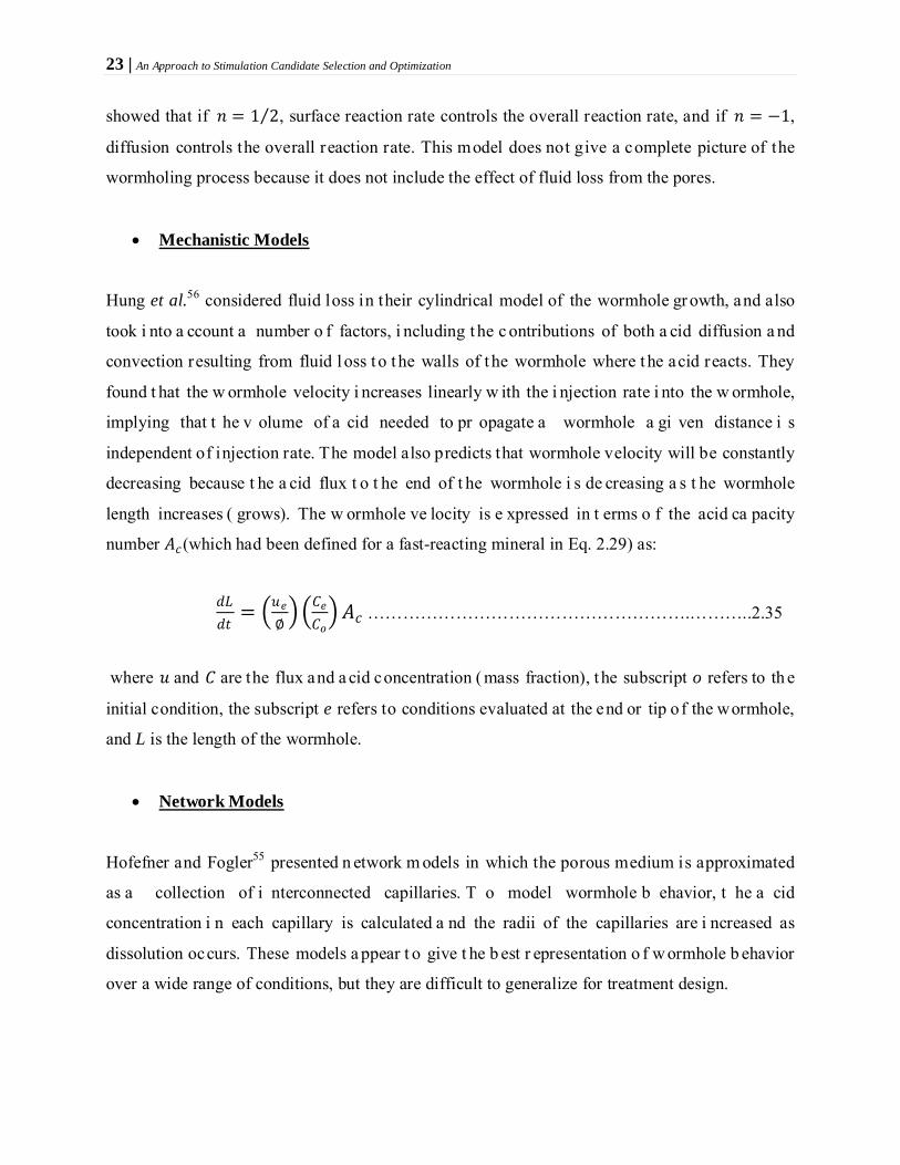
23 | An Approach to Stimulation Candidate Selection and Optimization
showed that if 𝑙𝑙 = 1 2⁄ , surface reaction rate controls the overall reaction rate, and if 𝑙𝑙 = −1,
diffusion controls the overall reaction rate. This model does not give a complete picture of the
wormholing process because it does not include the effect of fluid loss from the pores.
•
Mechanistic Models
Hung et al.56
considered fluid loss in their cylindrical model of the wormhole gr owth, and also
took i nto a ccount a number o f factors, i ncluding t he c ontributions of both a cid diffusion a nd
convection resulting from fluid l oss t o t he walls of t he wormhole where t he acid reacts. They
found t hat the w ormhole velocity i ncreases linearly w ith the i njection rate i nto the w ormhole,
implying that t he v olume of a cid needed to pr opagate a wormhole a gi ven distance i s
independent of injection rate. The model also predicts that wormhole velocity will be constantly
decreasing because t he a cid flux t o t he end of t he wormhole i s de creasing a s t he wormhole
length increases ( grows). The w ormhole ve locity is e xpressed in t erms o f the acid ca pacity
number 𝐴𝐴𝑐𝑐(which had been defined for a fast-reacting mineral in Eq. 2.29) as:
𝑑𝑑𝐿𝐿𝑑𝑑𝑡𝑡
= �𝑝𝑝𝑒𝑒∅� �𝐶𝐶𝑒𝑒
𝐶𝐶𝑝𝑝� 𝐴𝐴𝑐𝑐 ……………………………………………….………..2.35
where 𝑝𝑝 and 𝐶𝐶 are the flux and a cid concentration ( mass fraction), t he subscript o refers to th e
initial condition, the subscript e refers to conditions evaluated at the end or tip o f the wormhole,
and L is the length of the wormhole.
•
Network Models
Hofefner and Fogler55
presented n etwork m odels in which the porous medium is approximated
as a collection of i nterconnected capillaries. T o model wormhole b ehavior, t he a cid
concentration i n each capillary is calculated a nd the radii of the capillaries are i ncreased as
dissolution occurs. These models a ppear t o give t he b est r epresentation o f w ormhole b ehavior
over a wide range of conditions, but they are difficult to generalize for treatment design.
24 | An Approach to Stimulation Candidate Selection and Optimization
•
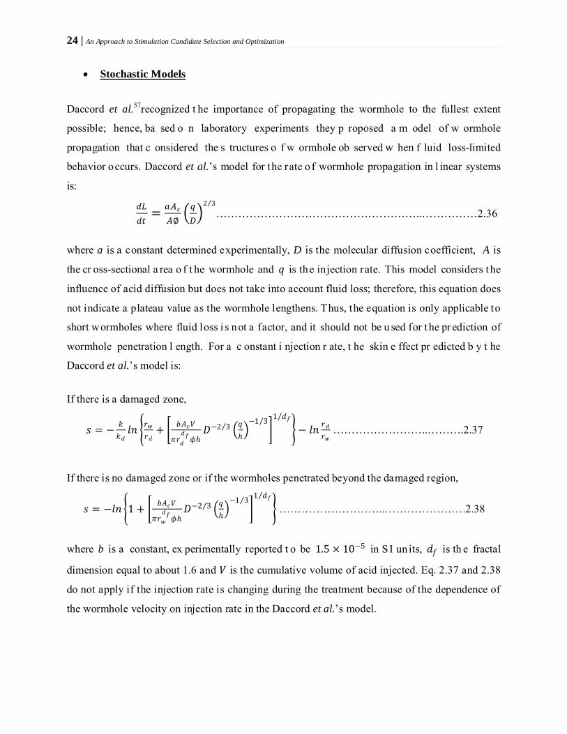
Stochastic Models
Daccord et al.57
𝑑𝑑𝐿𝐿𝑑𝑑𝑡𝑡
= 𝑎𝑎𝐴𝐴𝑐𝑐𝐴𝐴∅
�𝑒𝑒𝐷𝐷�
2 3⁄………………………………………………..……………2.36
recognized t he importance of propagating the wormhole to the fullest extent
possible; hence, ba sed o n laboratory experiments they p roposed a m odel of w ormhole
propagation that c onsidered the s tructures o f w ormhole ob served w hen f luid loss-limited
behavior occurs. Daccord et al.’s model for the rate o f wormhole propagation in l inear systems
is:
where a is a constant determined experimentally, D is the molecular diffusion coefficient, A is
the cr oss-sectional a rea o f t he wormhole and 𝑒𝑒 is the injection rate. This model considers t he
influence of acid diffusion but does not take into account fluid loss; therefore, this equation does
not indicate a plateau value as the wormhole lengthens. Thus, the equation is only applicable to
short wormholes where fluid loss i s not a factor, and it should not be u sed for t he pr ediction of
wormhole penetration l ength. For a c onstant i njection r ate, t he skin e ffect pr edicted b y t he
Daccord et al.’s model is:
If there is a damaged zone,
𝑠𝑠 = − 𝑘𝑘𝑘𝑘𝑑𝑑𝑙𝑙𝑙𝑙 �𝑟𝑟𝑤𝑤
𝑟𝑟𝑑𝑑+ � 𝑤𝑤𝐴𝐴𝑐𝑐𝑉𝑉
𝜋𝜋𝑟𝑟𝑑𝑑𝑑𝑑𝑓𝑓𝜙𝜙ℎ
𝐷𝐷−2 3⁄ �𝑒𝑒ℎ�−1 3⁄
�1 𝑑𝑑𝑓𝑓⁄
� − 𝑙𝑙𝑙𝑙 𝑟𝑟𝑑𝑑𝑟𝑟𝑤𝑤
……………………..……….2.37
If there is no damaged zone or if the wormholes penetrated beyond the damaged region,
𝑠𝑠 = −𝑙𝑙𝑙𝑙 �1 + � 𝑤𝑤𝐴𝐴𝑐𝑐𝑉𝑉
𝜋𝜋𝑟𝑟𝑤𝑤𝑑𝑑𝑓𝑓𝜙𝜙ℎ
𝐷𝐷−2 3⁄ �𝑒𝑒ℎ�−1 3⁄
�1 𝑑𝑑𝑓𝑓⁄
� ………………………..………………….2.38
where b is a constant, ex perimentally reported t o be 1.5 × 10⁻⁵ in S I un its, 𝑑𝑑𝑓𝑓 is th e fractal
dimension equal to about 1.6 and 𝑉𝑉 is the cumulative volume of acid injected. Eq. 2.37 and 2.38
do not apply if the injection rate is changing during the treatment because of the dependence of
the wormhole velocity on injection rate in the Daccord et al.’s model.
25 | An Approach to Stimulation Candidate Selection and Optimization
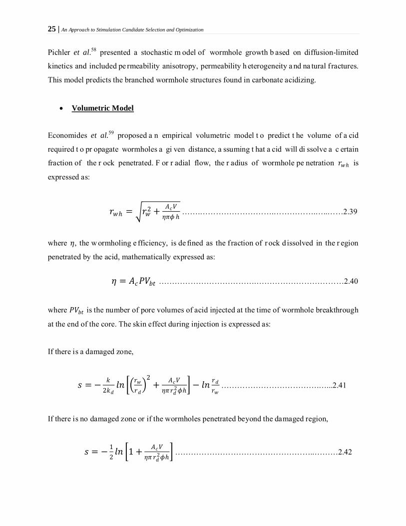
Pichler et al.58
presented a stochastic m odel of wormhole growth b ased on diffusion-limited
kinetics and included pe rmeability anisotropy, permeability h eterogeneity a nd na tural f ractures.
This model predicts the branched wormhole structures found in carbonate acidizing.
•
Volumetric Model
Economides et al.59
proposed a n empirical volumetric model t o predict t he volume of a cid
required t o pr opagate wormholes a gi ven distance, a ssuming t hat a cid will di ssolve a c ertain
fraction of the r ock penetrated. F or r adial flow, the r adius of wormhole pe netration 𝑟𝑟𝑤𝑤ℎ is
expressed as:
𝑟𝑟𝑤𝑤ℎ = �𝑟𝑟𝑤𝑤2 + 𝐴𝐴𝑐𝑐𝑉𝑉𝜂𝜂𝜋𝜋𝜙𝜙 ℎ
…….……………………….…………….…..……2.39
where 𝜂𝜂, the w ormholing e fficiency, is de fined as the fraction of r ock d issolved in the r egion
penetrated by the acid, mathematically expressed as:
𝜂𝜂 = 𝐴𝐴𝑐𝑐𝑃𝑃𝑉𝑉𝑤𝑤𝑡𝑡 ……………………………….……………………………2.40
where 𝑃𝑃𝑉𝑉𝑤𝑤𝑡𝑡 is the number of pore volumes of acid injected at the time of wormhole breakthrough
at the end of the core. The skin effect during injection is expressed as:
If there is a damaged zone,
𝑠𝑠 = − 𝑘𝑘2𝑘𝑘𝑑𝑑
𝑙𝑙𝑙𝑙 ��𝑟𝑟𝑤𝑤𝑟𝑟𝑑𝑑�
2+ 𝐴𝐴𝑐𝑐𝑉𝑉
𝜂𝜂𝜋𝜋𝑟𝑟𝑑𝑑2𝜙𝜙ℎ
� − 𝑙𝑙𝑙𝑙 𝑟𝑟𝑑𝑑𝑟𝑟𝑤𝑤
……………………………….…...2.41
If there is no damaged zone or if the wormholes penetrated beyond the damaged region,
𝑠𝑠 = − 12𝑙𝑙𝑙𝑙 �1 + 𝐴𝐴𝑐𝑐𝑉𝑉
𝜂𝜂𝜋𝜋 𝑟𝑟𝑑𝑑2𝜙𝜙ℎ
� ……………………………………………..………2.42
26 | An Approach to Stimulation Candidate Selection and Optimization
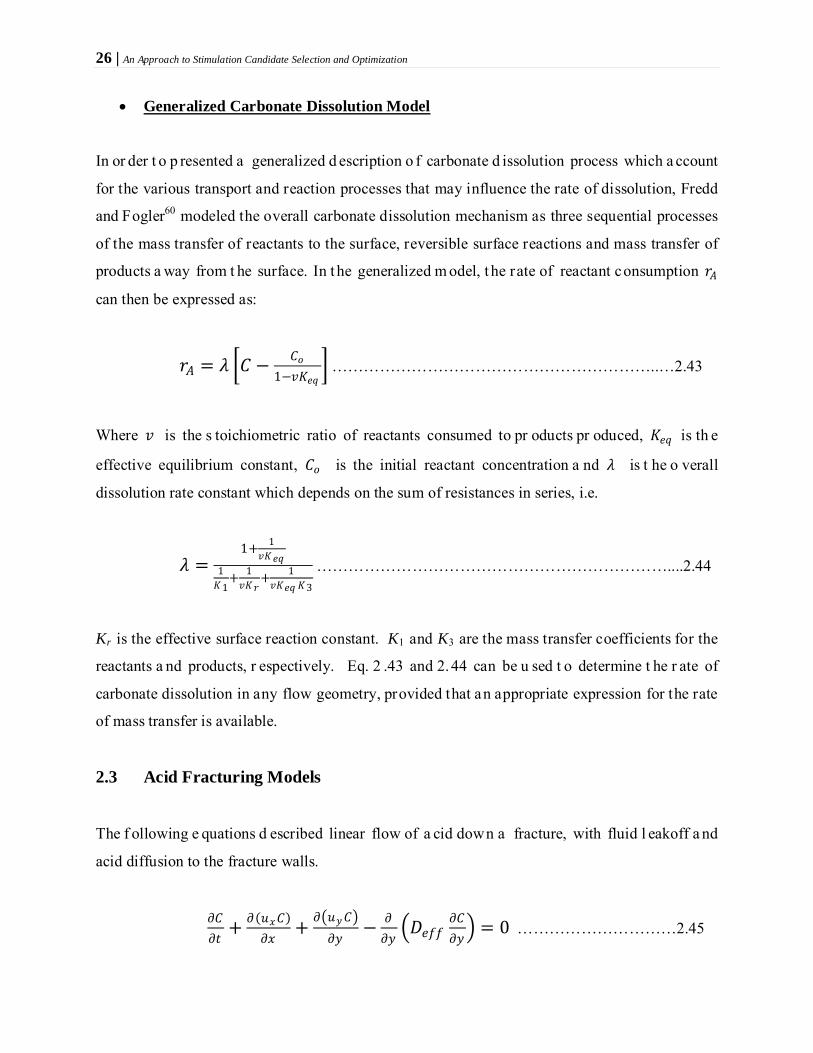
•
Generalized Carbonate Dissolution Model
In or der t o p resented a generalized d escription o f carbonate d issolution process which a ccount
for the various transport and reaction processes that may influence the rate of dissolution, Fredd
and Fogler60
modeled the overall carbonate dissolution mechanism as three sequential processes
of the mass transfer of reactants to the surface, reversible surface reactions and mass transfer of
products a way from t he surface. In t he generalized m odel, t he rate of reactant consumption 𝑟𝑟𝐴𝐴
can then be expressed as:
𝑟𝑟𝐴𝐴 = 𝜆𝜆 �𝐶𝐶 − 𝐶𝐶𝑝𝑝1−𝑣𝑣𝐾𝐾𝑒𝑒𝑒𝑒
� ……………………………………………………..…2.43
Where 𝑣𝑣 is the s toichiometric ratio of reactants consumed to pr oducts pr oduced, 𝐾𝐾𝑒𝑒𝑒𝑒 is th e
effective equilibrium constant, 𝐶𝐶𝑝𝑝 is the initial reactant concentration a nd 𝜆𝜆 is t he o verall
dissolution rate constant which depends on the sum of resistances in series, i.e.
𝜆𝜆 =1+ 1
𝑣𝑣𝐾𝐾𝑒𝑒𝑒𝑒1𝐾𝐾1
+ 1𝑣𝑣𝐾𝐾𝑟𝑟
+ 1𝑣𝑣𝐾𝐾𝑒𝑒𝑒𝑒 𝐾𝐾3
…………………………………………………………....2.44
Kr is the effective surface reaction constant. K1 and K3
are the mass transfer coefficients for the
reactants a nd products, r espectively. Eq. 2 .43 and 2.44 can be u sed t o determine t he r ate of
carbonate dissolution in any flow geometry, provided that an appropriate expression for the rate
of mass transfer is available.
2.3 Acid Fracturing Models
The f ollowing e quations d escribed linear flow of a cid down a fracture, with fluid l eakoff a nd
acid diffusion to the fracture walls.
𝜕𝜕𝐶𝐶𝜕𝜕𝑡𝑡
+ 𝜕𝜕(𝑝𝑝𝑚𝑚𝐶𝐶)𝜕𝜕𝑚𝑚
+ 𝜕𝜕�𝑝𝑝𝑑𝑑𝐶𝐶�𝜕𝜕𝑑𝑑
− 𝜕𝜕𝜕𝜕𝑑𝑑�𝐷𝐷𝑒𝑒𝑓𝑓𝑓𝑓
𝜕𝜕𝐶𝐶𝜕𝜕𝑑𝑑� = 0 …………………………2.45

27 | An Approach to Stimulation Candidate Selection and Optimization
𝐶𝐶(𝑚𝑚,𝑑𝑑, 𝑡𝑡 = 0) = 0 ………………………………2.46
𝐶𝐶(𝑚𝑚 = 0,𝑑𝑑, 𝑡𝑡) = 𝐶𝐶𝑎𝑎(𝑡𝑡) ………………………….2.47
𝐶𝐶𝑝𝑝𝑑𝑑 − 𝐶𝐶𝐿𝐿𝑒𝑒𝐿𝐿 − 𝐷𝐷𝑒𝑒𝑓𝑓𝑓𝑓𝜕𝜕𝐶𝐶𝜕𝜕𝑑𝑑
= 𝐹𝐹𝑓𝑓𝐶𝐶𝑙𝑙(1− ∅) ………...…….2.48
where 𝐶𝐶 is the acid concentration, 𝑝𝑝𝑚𝑚 is the flux along the fracture, 𝑝𝑝𝑑𝑑 is the transverse flux due
to fluid loss, 𝐷𝐷𝑒𝑒𝑓𝑓𝑓𝑓 is an effective diffusion coefficient, 𝐶𝐶𝑎𝑎 is the injected acid concentration, 𝐹𝐹𝑓𝑓 is
the r eaction rate co nstant, 𝑙𝑙 is t he or der of the r eaction, a nd ∅ is porosity. Ben-Naceur a nd
Economides61, Lo and Dean62, and Settari63 provided complex nu merical solutions t o t he a bove
equations considering c omplications s uch as t he temperature d istribution along the f racture,
viscous fingering of l ow-viscosity acid through a vi scous pad, the effect of the a cid on leak-off
behavior, a nd various fracture geometries. Neerode and Williams64
also pr esented a solution t o
the a bove e quations by a ssuming a steady state, laminar flow of a N ewtonian fluid between
parallel plates with constant fluid loss flux along the fracture. They presented the solution for the
concentration p rofile as a f unction of t he leakoff P eclet n umber. At l ow Peclet n umbers,
diffusion controls a cid propagation, while a t hi gh P eclet numbers, fluid l oss i s t he c ontrolling
factor.
The conductivity (𝑘𝑘𝑓𝑓𝑤𝑤) of an acid fracture depends on a stochastic process. Nierode and Kruk65
presented the following correlation for the acid fracture conductivity based on the ideal fracture
width 𝑤𝑤�𝑎𝑎 ,
𝑘𝑘𝑓𝑓𝑤𝑤 = 𝐶𝐶1𝑒𝑒−𝐶𝐶2𝜎𝜎𝑐𝑐 ……………………………………………………….2.49
where
𝐶𝐶1 = 1.47 × 10⁷𝑤𝑤𝑎𝑎2.47 ……………………………………………………2.50
and for
𝑆𝑆𝑟𝑟𝑝𝑝𝑐𝑐𝑘𝑘 < 20,000 psi: 𝐶𝐶2 = (13.9 − 1.3𝑙𝑙𝑙𝑙𝑆𝑆𝑟𝑟𝑝𝑝𝑐𝑐𝑘𝑘 ) × 10−3 ………………………….2.51

28 | An Approach to Stimulation Candidate Selection and Optimization
𝑆𝑆𝑟𝑟𝑝𝑝𝑐𝑐𝑘𝑘 > 20,000 psi: 𝐶𝐶2 = (13.9− 1.3𝑙𝑙𝑙𝑙𝑆𝑆𝑟𝑟𝑝𝑝𝑐𝑐𝑘𝑘 ) × 10−3 ………………………....2.52 In Eq. 2. 49 t hrough 2. 52, 𝜎𝜎𝑐𝑐 is the f racture closure s tress and 𝑆𝑆𝑟𝑟𝑝𝑝𝑐𝑐𝑘𝑘 is the r ock e mbedment
strength. The average ideal fracture width is defined as:
𝑤𝑤�𝑎𝑎 = 𝑋𝑋𝑉𝑉2(1−∅)ℎ𝑓𝑓𝑚𝑚𝑓𝑓
…………………………………………………………2.53
where 𝑋𝑋 is the volumetric dissolving power of the acid, 𝑉𝑉 is the total volume of acid injected, ℎ𝑓𝑓
is t he fracture height, a nd 𝑚𝑚𝑓𝑓 is the f racture h alf-length. The conductivity varies a long t he
fracture; hence Bennet66
defined an average conductivity (𝑘𝑘𝑓𝑓𝑤𝑤�����) that can be used to estimate the
productivity of the acid fracture well.
𝑘𝑘𝑓𝑓𝑤𝑤����� = 1𝑚𝑚𝑓𝑓∫ 𝑘𝑘𝑓𝑓𝑚𝑚𝑓𝑓
0 𝑤𝑤𝑑𝑑𝑚𝑚 …………………………………………….….2.54
For lower values of Peclet number (< 3), this average overestimate the well productivity, hence
Ben-Naceur and Economides67
presented a harmonic a verage which better a pproximates the
behavior of the fractured well as:
𝑘𝑘𝑓𝑓𝑤𝑤����� = 𝑚𝑚𝑓𝑓
∫ 𝑑𝑑𝑚𝑚/𝑘𝑘𝑓𝑓𝑚𝑚𝑓𝑓
0 𝑤𝑤 ……………………………………………………..2.55
Ben-Naceur and Economides67
also presented a series of performance type curves for a cid-
fractured wells producing at a constant bottomhole flowing pressure of 500 psi.
2.4 Hydraulic Fracturing Models
Hydraulics fractures c an b e c lassified a ccording to one of three m odels: infinite conductivity
model (assuming no pressure loss in the fracture), uniform flux model (assumes a slight pressure
gradient i n t he fracture), a nd finite c onductivity m odel (assumes co nstant a nd l imited
permeability i n the fracture f rom proppant crushing o r p oor pr oppant distribution). Every
hydraulic fracture i s characterized by i ts l ength, conductivity a nd r elated equivalent skin effect.
29 | An Approach to Stimulation Candidate Selection and Optimization
The fracture length, which is the conductive length and not the hydraulic length, is assumed to be
consisting of t wo e qual half-lengths, 𝑚𝑚𝑓𝑓 in e ach s ide of the w ell. Prats68
provided p ressure
profiles in a fractured r eservoir as a function of t he f racture h alf-length 𝑚𝑚𝑓𝑓 and t he relative
capacity, a, which he defined as:
𝑎𝑎 = 𝜋𝜋𝑘𝑘𝑚𝑚𝑓𝑓2𝑘𝑘𝑓𝑓𝑤𝑤
………………………………………………..………………2.56
where 𝑘𝑘 is the r eservoir p ermeability, 𝑘𝑘𝑓𝑓 is t he fracture permeability, a nd 𝑤𝑤 is t he propped
fracture w idth. A rgawal et al.69 and C inco-Ley and Samaniego70
introduced t he dimensionless
fracture conductivity, 𝐹𝐹𝐶𝐶𝐷𝐷 which is defined as:
𝐹𝐹𝐶𝐶𝐷𝐷 = 𝑘𝑘𝑓𝑓𝑤𝑤𝑘𝑘𝑚𝑚𝑓𝑓
.. ……………………………………………………..…….2.57
The dimensionless fracture conductivity 𝐹𝐹𝐶𝐶𝐷𝐷 is related to the relative capacity 𝑎𝑎 by:
𝐹𝐹𝐶𝐶𝐷𝐷 = 𝜋𝜋2𝑎𝑎
………………………………………………………….…...2.58
Prats68
𝑟𝑟𝑤𝑤𝐷𝐷́ = 𝑟𝑟�́�𝑤𝑚𝑚𝑓𝑓
………………………………………………...…………2.59
showed t hat for a s teady-state f low, a fracture affects productivity t hrough t he
dimensionless equivalent (effective) wellbore r adius 𝑟𝑟𝑤𝑤𝐷𝐷́ which i s related t o the fracture half-
length or penetration 𝑚𝑚𝑓𝑓 by the dimensionless fracture conductivity 𝐹𝐹𝐶𝐶𝐷𝐷 .
where 𝑟𝑟�́�𝑤 is expressed in terms of the equivalent skin effect 𝑠𝑠𝑓𝑓 and the wellbore radius 𝑟𝑟𝑤𝑤 as:
𝑟𝑟�́�𝑤 = 𝑟𝑟𝑤𝑤𝑒𝑒−𝑠𝑠𝑓𝑓 …...................................................................................2.60
For infinite conductivity fractures, Prats68
showed that:
𝑟𝑟�́�𝑤 = 0.5𝑚𝑚𝑓𝑓 ……………………………………………….…………2.61
30 | An Approach to Stimulation Candidate Selection and Optimization
Cinco-Ley et al.71
integrated t his i nto a full description of r eservoir r esponse by i ncluding
transient f low and pseudoradial flow ( where t he pressure-depletion r egion >> 𝑚𝑚𝑓𝑓 but i s not
affected by e xternal boundaries). Cinco-Ley et al.’s descriptions presented in form of charts can
be used a s powerful reservoir engineering tools to assess p ossible post-fracture p roductivity
benefits from propped fracturing. The productivity index 𝐽𝐽 in the pseudosteady state flow regime
is expressed as:
𝐽𝐽 = 2𝜋𝜋𝑘𝑘ℎ𝑞𝑞𝜇𝜇
× 1
ln 0.472𝑟𝑟𝑒𝑒+0.5𝑙𝑙𝑙𝑙 ℎ𝑘𝑘𝑉𝑉𝑓𝑓𝑘𝑘𝑓𝑓
+�0.5𝑙𝑙𝑙𝑙𝐹𝐹𝐶𝐶𝐷𝐷 +𝑠𝑠𝑓𝑓+𝑙𝑙𝑙𝑙𝑚𝑚𝑓𝑓𝑟𝑟𝑤𝑤� …....................................2.62
𝐹𝐹𝐶𝐶𝐷𝐷 = 1.6, is t he optimum value of the dimensionless fracture conductivity for which the
productivity index 𝐽𝐽 is maximum.
2.5 Literatures on Stimulation Candidate Selection
Several techniques for stimulation candidate selection exist in l iteratures a nd a lso i n practice i n
the i ndustries. Stimulation jobs ha ve w itnessed bot h s uccesses and f ailures, and in s ome c ases
yield less than the expected result. Stimulation failure is usually due to poor candidate selection,
inaccurate treatment de sign or improper f ield pr ocedures72. Nnanna et al.73
cautioned t hat
applying t he b est t reatment d esign a nd field pr ocedures t o t he wrong candidate w ill r esult i n a
failure, while a poor treatment design and good field procedures on the right candidate will also
result in a failure. They a dded that t hough treatment design and field pr ocedures a re fairly well
understood, candidate selection ha s been approached in different ways by various operators and
service companies.
Nitters et al.74
presented a structured a pproach t o stimulation candidate selection and treatment
design. T hey i solated t he r eal skin caused b y da mage ( the p ortion o f t he t otal skin t hat can b e
removed by matrix treatment) from the total skin as follows:
𝑠𝑠𝑑𝑑𝑎𝑎𝑚𝑚 = 𝑠𝑠𝑡𝑡𝑝𝑝𝑡𝑡 − �𝑠𝑠𝑝𝑝𝑒𝑒𝑟𝑟𝑓𝑓 + 𝑠𝑠𝑡𝑡𝑝𝑝𝑟𝑟𝑤𝑤 + 𝑠𝑠𝑑𝑑𝑒𝑒𝑣𝑣 + 𝑠𝑠𝑙𝑙𝑟𝑟𝑎𝑎𝑣𝑣 𝑒𝑒𝑙𝑙 + 𝑠𝑠𝑝𝑝𝑒𝑒𝑟𝑟𝑓𝑓 𝑠𝑠𝑎𝑎𝑠𝑠𝑒𝑒 � ………..….2.63

31 | An Approach to Stimulation Candidate Selection and Optimization
where 𝑠𝑠𝑑𝑑𝑎𝑎𝑚𝑚 is the skin due to formation damage, 𝑠𝑠𝑡𝑡𝑝𝑝𝑡𝑡 is the total skin factor (Eq. 2 .1), 𝑠𝑠𝑝𝑝𝑒𝑒𝑟𝑟𝑓𝑓 is
the skin resulting from limited perforation height, 𝑠𝑠𝑡𝑡𝑝𝑝𝑟𝑟𝑤𝑤 is the skin due to turbulent (non-Darcy)
flow, 𝑠𝑠𝑑𝑑𝑒𝑒𝑣𝑣 is t he skin du e t o wellbore deviation, 𝑠𝑠𝑙𝑙𝑟𝑟𝑎𝑎𝑣𝑣𝑒𝑒𝑙𝑙 is the skin due to gravel packing, and
𝑠𝑠𝑝𝑝𝑒𝑒𝑟𝑟𝑓𝑓 𝑠𝑠𝑎𝑎𝑠𝑠𝑒𝑒 is the skin resulting from a small perforation. Nitters et al then suggested the ranking of
stimulation candidates based on the magnitude of the damage skin factor.
Jones75
presented a nalytical r elationship which i s convenient t o estimate productivity
improvement achievable by skin removal. At equal pressure and also approximating 𝑙𝑙𝑙𝑙(𝑟𝑟𝑒𝑒 𝑟𝑟𝑤𝑤⁄ ) to
7, Jones defined the ratio of rates before and after stimulation (the stimulation ratio, 𝐹𝐹𝑠𝑠) as:
𝐹𝐹𝑠𝑠 = 𝑒𝑒2
𝑒𝑒1= 7+𝑠𝑠1
7+𝑠𝑠2 …………………………………………………….2.64
where 𝑒𝑒 is flow ra te, 𝑠𝑠 is the skin factor, and t he subscripts 1 and 2 refer t o before and a fter
stimulation.
To properly interpret t he skin and t herefore determine t he appropriate r emedial action r equires
analysis of t he contributing factors. Nnanna and Ajienka76 used the simplified approach for
determining the c ompletion s kin f actor as developed b y A l Qahtani a nd A l Shehri77 in
combination w ith t he non-linear summation r elationship between the pseudoskins and the t otal
skin as demonstrated by Yildiz78 to present a method for stimulation candidate selection. Nnanna
and Ajienka expressed the removable skin factor in the form presented by Lee79
as:
𝑆𝑆𝑑𝑑 = ℎ𝑝𝑝ℎ
(𝑆𝑆𝑇𝑇 + 𝑆𝑆𝑐𝑐+𝜃𝜃 )− 𝑆𝑆𝑝𝑝 …………………………………………2.65
where 𝑆𝑆𝑐𝑐+𝜃𝜃 is the skin factor due to partial penetration and deviation, 𝑆𝑆𝑇𝑇 is the total skin
factor as d eternmined f rom a w ell t est. 𝑆𝑆𝑝𝑝 is t he perforation skin factor. hp is th e perforation
interval thickness and h is the thickness of the oil sand. They used the stabilized inflow equation,
approximating the natural logarithm of t he ratio of drainage radius t o wellbore radius as 8 , a nd
the cu t-off of O nyekonwu80
to define a simplified R -factor which c an b e used for c andidate
selection. The factor is defined as:
32 | An Approach to Stimulation Candidate Selection and Optimization
𝐷𝐷 = ℎℎ𝑝𝑝∗ 𝑆𝑆𝑑𝑑
8+𝑆𝑆 …………………….………............................................ 2.66
They concluded that if R ≥ 0.6, then the well is a good stimulation candidate in the Niger Delta.
Afolabi et al.81
also presented candidate selection criterion that is based on minimum economic
reserve, productivity Index (PI) of less than 10bpd/psi, flow efficiency of less than 0.5 and the PI
decline rate that is greater than 30%.
Jennings82
presented a methodology for candidate selection ba sed o n w ell c apacity a nd
concluded that well stimulation tr eatments in high-productivity wells a llow better r eservoir
management through sustained productivity and more uniform reservoir depletion throughout the
life of the well, and that good wells make better candidates for matrix stimulation.
Kartoatmodjo et al.83 presented a risk-based c andidate selection a pproach by c onsidering the
range of probability of all the possible outcomes in a stimulation campaign using Monte Carlo
simulation technique. They concluded that decision risk analysis is a valuable tool for candidate
selection. Stimulation c andidate selection c ampaign ba sed on highest expected ga in a nd/or
lowest expected risk has also been reported.
84
The published literatures reviewed did not consider a detailed and efficient optimization process
for s timulation candidate selection, especially i n t he N iger D elta, a nd hence t he n eed f or this
study.
33 | An Approach to Stimulation Candidate Selection and Optimization
Chapter Three
Methodology This methodology is a modification of the modular approach to stimulation decisions presented
by S inson et al.85
The m odels pr esented are de rived f rom i ndustry-wide a ccepted well
stimulation procedures and techniques.
3.1 Well Screening Technique
It i s a ssumed that from well t est da ta, t he well pr oblem could b e diagnosed a nd then matched
with either of acidizing, gravel-packing or re-completion. It is also assumed that all wells can be
acidized, recompleted or gravel-packed successfully if necessary.
Diagnose each well pr oblem. For w ells w ith s kin va lues s howing formation da mage problems,
acidizing i s t he r ecommended t reatment. Wells with m echanical pr oblems s uch a s pa rtially or
totally plugged perforations, i nsufficient perforation density, l ow depth of perforation o r water
production, r e-completion i s r ecommended. I f t he pr oblem i s sand production, t hen gravel
packing i s r ecommended. A s imple screening module flow chart f or t his s ection i s s hown i n
Appendix A.
3.2 Design of Stimulation Treatment Models
The treatment m odels p resented in t his s ection are to b e used f or the s timulation t reatment
design. The choice of which model to use is dependent on the nature of well problem diagnosed
and the result of the screening module.
3.2.1 Matrix Acidizing Design Model
The extent t o which acid will penetrate a rock is dependent on both the rock properties and the
local acid reaction rate. The reaction rate in turn depends on matrix properties and other variables
like temperature, pressure, and composition of the reacting fluids.

34 | An Approach to Stimulation Candidate Selection and Optimization
The m odel p resented here i s a c ombination o f t he a pproaches presented b y S chechter a nd
Gidley32 and E conomides a nd N olte86
. I n t his model, pores ar e a ssumed to be i nterconnected
such that the acid can flow through the matrix under the influence of a pressure gradient.
The Niger Delta formation is c hiefly made up of sandstone. S andstone formations are of ten
treated with a mixture of hydrochloric a cid (HCl) and hydrofluoric a cid ( HF) commonly called
mud acids. T he t reatment is done at l ow injection rate to prevent fracturing. The mud acid,
chosen because of its ability to dissolve the clay found in drilling mud, also will react with most
constituent of naturally occurring sandstones, including silica, feldspar, and calcareous materials.
The following steps are presented for sandstone acidizing design:
• Determine the present fracture gradient for the well. If the instantaneous shut-in
pressure value is not available, use the following equation to calculate the fracture
gradient:
𝑔𝑔𝑓𝑓 = 𝛼𝛼 + (𝑔𝑔𝑜𝑜𝑜𝑜 − 𝛼𝛼) 𝑃𝑃𝑟𝑟𝐷𝐷
…………………………………………….….3.1
where:
𝑔𝑔𝑓𝑓 = fracture gradient, psi/ft
𝛼𝛼 = 0.33 to 0.50 psi/ft
𝑔𝑔𝑜𝑜𝑜𝑜 = overburden gradient (1.0 psi/ft for formation depth 𝐷𝐷 less than 10,000ft or 1.2 psi/ft
for depth greater than 10,000ft)
𝑃𝑃𝑟𝑟 = reservoir pressure, psi
𝐷𝐷 = depth of formation, ft
• Predict the maximum possible injection rate that does not fracture the formation
using:
𝑞𝑞𝑖𝑖 ,𝑚𝑚𝑚𝑚𝑚𝑚 = 4.917×10⁻⁶𝑘𝑘ℎ��𝑔𝑔𝑓𝑓×𝐷𝐷�−∆𝑃𝑃𝑠𝑠𝑚𝑚𝑓𝑓𝑠𝑠 −𝑃𝑃𝑟𝑟�
𝜇𝜇𝜇𝜇 �𝑙𝑙𝑙𝑙�𝑟𝑟𝑠𝑠𝑟𝑟𝑤𝑤�+𝑠𝑠�
…………………………………….3.2
where:
𝑞𝑞𝑖𝑖,𝑚𝑚𝑚𝑚𝑚𝑚 = injection rate, bbl/min

35 | An Approach to Stimulation Candidate Selection and Optimization
𝑘𝑘 = effective permeability of the undamaged formation, md
ℎ = net pay thickness, ft
∆𝑃𝑃𝑠𝑠𝑚𝑚𝑓𝑓𝑠𝑠 = safety margin for the pressure, psi (usually 200 to 500 psi)
𝜇𝜇 = viscosity of the injected fluid, cp
𝑟𝑟𝑠𝑠 = drainage radius, ft
𝑟𝑟𝑤𝑤 = wellbore radius, ft
𝑠𝑠 = skin factor, dimensionless
𝜇𝜇 = formation volume factor, bbl/STB (it has a value of 1 for incompressible fluids)
Using Equation 3.2 with zero value for the skin effect 𝑠𝑠 gives the maximum pump rate during the
treatment.
• Estimate the pipe or coil tubing friction pressure gradient
If the injection fluid is Newtonian, and at pumping rates that are less than 9 bbl/min, t he coil
tubing friction pressure can be calculated using:
𝑔𝑔𝑓𝑓𝑟𝑟𝑖𝑖𝑓𝑓𝑓𝑓𝑖𝑖𝑜𝑜𝑙𝑙 = 0.518𝛾𝛾0.79𝑞𝑞1.79𝜇𝜇0.207
𝑑𝑑4.79 ………………………………….……….…….3.3
where:
𝑔𝑔𝑓𝑓𝑟𝑟𝑖𝑖𝑓𝑓𝑓𝑓𝑖𝑖𝑜𝑜𝑙𝑙 = frictional pressure, psi/ft
𝛾𝛾 = specific gravity of the acid (or density of acid in g/cc)
𝑞𝑞 = pump rate, bbl/min
𝑑𝑑 = diameter of pipe, inches
This friction pressure component should be ignored if the pumping rate is greater than 9 bbl/min.
• Predict maximum surface pressure.
If p ipe or c oil tubing f riction pressure is co nsidered, the maximum s urface p ressure f or w hich
fluids can be injected without fracturing the formation is calculated using:

36 | An Approach to Stimulation Candidate Selection and Optimization
𝑃𝑃𝑠𝑠 ,𝑚𝑚𝑚𝑚𝑚𝑚 = �𝑔𝑔𝑓𝑓 + 𝑔𝑔𝑓𝑓𝑟𝑟𝑖𝑖𝑓𝑓𝑓𝑓𝑖𝑖𝑜𝑜𝑙𝑙 − 𝑔𝑔𝑚𝑚𝑓𝑓𝑖𝑖𝑑𝑑 �𝐷𝐷 ………………………………………...3.4
where:
𝑔𝑔𝑚𝑚𝑓𝑓𝑖𝑖𝑑𝑑 = acid hydrostatic gradient, psi/ft
If pipe or coil tubing friction pressure is ignored, then
𝑃𝑃𝑠𝑠,𝑚𝑚𝑚𝑚𝑚𝑚 = �𝑔𝑔𝑓𝑓 − 𝑔𝑔𝑚𝑚𝑓𝑓𝑖𝑖𝑑𝑑 �𝐷𝐷 ……………………………………….….……………3.5
• Determine the volume of mud acid to use
It i s a ssumed that t he a cid volume r equired is equal to the pore volume of t he damaged zone.
Also, i t i s a ssumed that a cid flows t hrough the porous media with a front t hat i s u niform a nd
stable, then the acid injection is piston-like and the first acid in is the last acid out. The mud acid
volume is estimated using:
𝑉𝑉𝑚𝑚 = 7.48[𝜋𝜋∅(𝑟𝑟𝑠𝑠2 − 𝑟𝑟𝑤𝑤2)] ……………………………………………………...3.6
where:
𝑉𝑉𝑚𝑚 = volume of mud acid, gal/ft
∅ = porosity, fraction
𝑟𝑟𝑠𝑠 = damaged radius (displaced section), ft
In formations where the HCl solubility is moderate to high more HCl is necessary. The following
equation is used to calculate this volume and address the HCl-soluble materials:
𝑉𝑉𝐻𝐻𝐻𝐻𝑙𝑙 = 7.48 𝜋𝜋(1−∅)𝑋𝑋𝐻𝐻𝐻𝐻𝑙𝑙 [𝑟𝑟𝑠𝑠2−𝑟𝑟𝑤𝑤2 ]𝛽𝛽
……………………………………………..3.7
where:
𝑉𝑉𝐻𝐻𝐻𝐻𝑙𝑙 = volume of HCl required, gal/ft

37 | An Approach to Stimulation Candidate Selection and Optimization
𝑋𝑋𝐻𝐻𝐻𝐻𝑙𝑙 = fraction of the bulk rock dissolved by HCl
𝛽𝛽 = dissolving coefficient, expressed as amount of rock dissolved per gallon of acid
• Specify the acid treatment
a. Preflush
Normally, inject 50 gallons of regular acid per foot of perforation interval.
b. Mud Acid
Inject the volume of mud acid calculated from Equation 3.6.
c. Afterflush
In oil wells, inject a volume of diesel oi l or hydrochloric acid equal to the mud acid
volume.
• Calculate cost of sandstone matrix acidizing
𝐻𝐻𝑠𝑠 = 𝑓𝑓𝑠𝑠𝑚𝑚 × 𝑉𝑉ℎ ……………………………………………………..3.8
where:
𝑓𝑓𝑠𝑠𝑚𝑚 = cost of acid used per unit volume, $/gal
• Calculate the maximum productivity ratio
In sandstone it is difficult to increase the permeability above the natural state because of reaction
kinetics li mitations, r eaction stoichiometry a nd economics. In th is th esis, the maximum
formation productivity r atio for sandstone acidizing, given some set of reservoir parameters, is
defined by the reciprocal of the flow efficiency, and is approximated from Equation 2.21, using
the semi-steady state definition:
38 | An Approach to Stimulation Candidate Selection and Optimization
𝐹𝐹𝑚𝑚𝑚𝑚𝑚𝑚 =𝑙𝑙 𝑙𝑙�0.472𝑟𝑟𝑠𝑠
𝑟𝑟𝑤𝑤�+𝑠𝑠
𝑙𝑙 𝑙𝑙�0.472𝑟𝑟𝑠𝑠𝑟𝑟𝑤𝑤
�………………………………………………..……3.9
where:
𝐹𝐹𝑚𝑚𝑚𝑚𝑚𝑚 = maximum productivity ratio, dimensionless
𝑠𝑠 = skin factor (defined in Equation 2.1), dimensionless
3.2.1.1 Summary
1. Determine the present fracture gradient for the well.
2. Predict the maximum possible injection rate that does not fracture the formation.
3. Estimate the pipe or coil tubing friction pressure gradient.
4. Predict maximum surface pressure.
5. Determine the volume of mud acid to use.
6. Specify the acid treatment.
7. Calculate cost of sandstone matrix acidizing
8. Calculate the maximum productivity ratio.
3.2.2 Recompletion Design Model
The approach considered in this section assumes that the well is already completed. The concept
of recompletion is either t o increase the perforation density or increase the depth of perforation
penetration in order to increase production. The procedure presented below is based on the works
of Strubhar et al.87
• Calculate the skin due to perforation geometry
𝑠𝑠𝑝𝑝 = � ℎℎ𝑝𝑝− 1��𝑙𝑙𝑙𝑙 ℎ
𝑟𝑟𝑤𝑤− 2� …………………………………………….3.10
where:
ℎ = total formation thickness, ft
ℎ𝑝𝑝 = perforated interval length, ft
𝑟𝑟𝑤𝑤 = wellbore radius, ft
39 | An Approach to Stimulation Candidate Selection and Optimization
• Calculate the perforation damage
𝑠𝑠𝑑𝑑𝑝𝑝 = � ℎ𝐿𝐿𝑝𝑝𝑙𝑙
� �𝑙𝑙𝑙𝑙 𝑟𝑟𝑑𝑑𝑝𝑝𝑟𝑟𝑝𝑝� � 𝑘𝑘𝑟𝑟
𝑘𝑘𝑑𝑑𝑝𝑝− 𝑘𝑘𝑟𝑟
𝑘𝑘𝑑𝑑� ……………………………….……..3.11
where:
𝑟𝑟𝑑𝑑𝑝𝑝 = 𝑟𝑟𝑝𝑝 + 0.5 ………………………………………………..…3.12
𝑘𝑘𝑟𝑟𝑘𝑘𝑑𝑑𝑝𝑝
= 10.03
………………………………………………………..3.13
and:
𝐿𝐿𝑝𝑝 = depth of penetration in rock, ft
𝑙𝑙 = number of perforations
𝑟𝑟𝑑𝑑𝑝𝑝 = radius of compacted zone around the perforations, ft
𝑟𝑟𝑝𝑝 = radius of perforation in rock, ft
𝑘𝑘𝑟𝑟 = reservoir permeability, md
𝑘𝑘𝑑𝑑𝑝𝑝 = permeability of compacted zone around perforation in rock, md
• Calculate the total skin
𝑠𝑠 = 𝑠𝑠𝑝𝑝 + 𝑠𝑠𝑑𝑑𝑝𝑝 …………………………………………………………3.14
• Calculate cost of recompletion
𝐻𝐻𝑅𝑅 = 𝑓𝑓𝑝𝑝𝑠𝑠𝑟𝑟𝑓𝑓 × 𝑙𝑙𝑝𝑝𝑠𝑠𝑟𝑟𝑓𝑓 …………….……….……………………….……3.15
where:
𝑓𝑓𝑝𝑝𝑠𝑠𝑟𝑟𝑓𝑓 = cost per perforation, $
𝑙𝑙𝑝𝑝𝑠𝑠𝑟𝑟𝑓𝑓 = number of perforations
40 | An Approach to Stimulation Candidate Selection and Optimization
• Calculate the maximum productivity ratio
The productivity index for a semi-steady state condition is used to define the productivity ratio,
and hence, defining the productivity ratio as the reciprocal of the flow efficiency, it is expressed
as:
𝐹𝐹𝑚𝑚𝑚𝑚𝑚𝑚 =𝑙𝑙 𝑙𝑙�0.472𝑟𝑟𝑠𝑠
𝑟𝑟𝑤𝑤�+𝑠𝑠
𝑙𝑙 𝑙𝑙�0.472𝑟𝑟𝑠𝑠𝑟𝑟𝑤𝑤
� …………………………………...…………………3.16
where:
𝑠𝑠 = total skin factor calculated from Equation 3.14
3.2.3 Gravel-Pack Design Model
The f ollowing gravel pa ck d esign m odule is modified from Schlumberger’s gravel pack design
and c alculation m anual. The vo lume of g ravel r equired i s de pendent o n t he formation
permeability, to tal l ength o f t he in terval a nd t he c ondition of th e well ( i.e. whether it i s a n ew
well or an old well). The ideal situation is that all perforation tunnels and screen casing annulus
be filled with gravel. The gravel pack design considered is for re-completion of zones that have
produced sands. The following steps are considered in the design.
• Calculate the blank/casing annular volume
100% or less of t his volume m ay be c onsidered as the e xcess g ravel. T his volume e nsures
complete screen/formation coverage by the gravel.
𝑉𝑉1 = 𝜋𝜋4×144
�𝐼𝐼𝐷𝐷𝑓𝑓𝑠𝑠𝑔𝑔2 −𝑂𝑂𝐷𝐷𝑜𝑜𝑙𝑙𝑚𝑚𝑙𝑙𝑘𝑘2 �𝐿𝐿𝑜𝑜𝑙𝑙𝑚𝑚𝑙𝑙𝑘𝑘 …………………………………3.17
where:
𝑉𝑉1 = blank/casing annular volume, ft3
𝐼𝐼𝐷𝐷𝑓𝑓𝑠𝑠𝑔𝑔 = inner diameter of the casing string, inches
𝑂𝑂𝐷𝐷𝑜𝑜𝑙𝑙𝑚𝑚𝑙𝑙𝑘𝑘 = outer diameter of the blank string, inches
41 | An Approach to Stimulation Candidate Selection and Optimization
𝐿𝐿𝑜𝑜𝑙𝑙𝑚𝑚𝑙𝑙𝑘𝑘 = length of the blank string, ft
• Calculate the screen/casing annular volume
This volume must be filled up completely with gravel in order to have an efficient pack.
𝑉𝑉2 = 𝜋𝜋4×144
�𝐼𝐼𝐷𝐷𝑓𝑓𝑠𝑠𝑔𝑔2 − 𝑂𝑂𝐷𝐷𝑠𝑠𝑓𝑓𝑟𝑟𝑠𝑠𝑠𝑠𝑙𝑙2 �𝐿𝐿𝑠𝑠𝑓𝑓𝑟𝑟𝑠𝑠𝑠𝑠𝑙𝑙 ………………………….…3.18
where:
𝑉𝑉2 = screen/casing annular volume, ft3
𝑂𝑂𝐷𝐷𝑠𝑠𝑓𝑓𝑟𝑟𝑠𝑠𝑠𝑠𝑙𝑙 = outer diameter of the screen, inches
𝐿𝐿𝑠𝑠𝑓𝑓𝑟𝑟𝑠𝑠𝑠𝑠𝑙𝑙 = length of the screen, ft
• Calculate the volume of gravel to be injected into perforations
This is the volume of gravel required to pack the perforations.
𝑉𝑉3 = 𝐻𝐻𝑝𝑝 ∗ ℎ𝑝𝑝𝑠𝑠𝑟𝑟𝑓𝑓 ………………………………………………………..3.19
where:
𝑉𝑉3 = volume of gravel injected into perforations, ft
𝐻𝐻𝑝𝑝 = 0.5 – 1.5 ft
3 3
ℎ𝑝𝑝𝑠𝑠𝑟𝑟𝑓𝑓 = vertical height of perforated interval, ft
/ft (for the zones that have produced sands).
• Calculate total volume of gravel needed
𝑉𝑉𝑔𝑔 = 𝑉𝑉1 ∗ (𝑚𝑚) + 𝑉𝑉2 + 𝑉𝑉3 …………………………………………………3.20
where:
𝑉𝑉𝑔𝑔 = total volume of gravel needed, ft
𝑚𝑚 = fraction of the blank/casing annulus needed to be filled (in this thesis, taken to
3
be 60% - 90%)
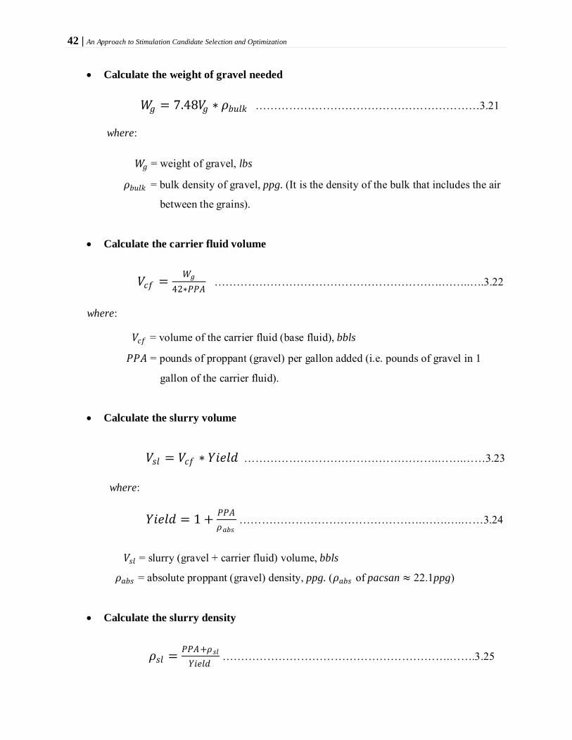
42 | An Approach to Stimulation Candidate Selection and Optimization
• Calculate the weight of gravel needed
𝑊𝑊𝑔𝑔 = 7.48𝑉𝑉𝑔𝑔 ∗ 𝜌𝜌𝑜𝑜𝑏𝑏𝑙𝑙𝑘𝑘 ……………………………………………………3.21
where:
𝑊𝑊𝑔𝑔 = weight of gravel, lbs
𝜌𝜌𝑜𝑜𝑏𝑏𝑙𝑙𝑘𝑘 = bulk density of gravel, ppg. (It is the density of the bulk that includes the air
between the grains).
• Calculate the carrier fluid volume
𝑉𝑉𝑓𝑓𝑓𝑓 = 𝑊𝑊𝑔𝑔
42∗𝑃𝑃𝑃𝑃𝑃𝑃 …………………………………………………….……..….3.22
where:
𝑉𝑉𝑓𝑓𝑓𝑓 = volume of the carrier fluid (base fluid), bbls
𝑃𝑃𝑃𝑃𝑃𝑃 = pounds of proppant (gravel) per gallon added (i.e. pounds of gravel in 1
gallon of the carrier fluid).
• Calculate the slurry volume
𝑉𝑉𝑠𝑠𝑙𝑙 = 𝑉𝑉𝑓𝑓𝑓𝑓 ∗ 𝑌𝑌𝑖𝑖𝑠𝑠𝑙𝑙𝑑𝑑 …………………………………………….…….……3.23
where:
𝑌𝑌𝑖𝑖𝑠𝑠𝑙𝑙𝑑𝑑 = 1 + 𝑃𝑃𝑃𝑃𝑃𝑃𝜌𝜌𝑚𝑚𝑜𝑜𝑠𝑠
………………………………………….…….….……3.24
𝑉𝑉𝑠𝑠𝑙𝑙 = slurry (gravel + carrier fluid) volume, bbls
𝜌𝜌𝑚𝑚𝑜𝑜𝑠𝑠 = absolute proppant (gravel) density, ppg. (𝜌𝜌𝑚𝑚𝑜𝑜𝑠𝑠 of pacsan ≈ 22.1ppg)
• Calculate the slurry density
𝜌𝜌𝑠𝑠𝑙𝑙 = 𝑃𝑃𝑃𝑃𝑃𝑃+𝜌𝜌𝑠𝑠𝑙𝑙𝑌𝑌𝑖𝑖𝑠𝑠𝑙𝑙𝑑𝑑
…………………………………………………….…….3.25
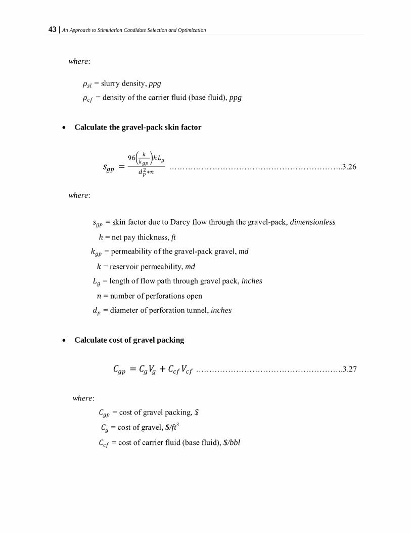
43 | An Approach to Stimulation Candidate Selection and Optimization
where:
𝜌𝜌𝑠𝑠𝑙𝑙 = slurry density, ppg
𝜌𝜌𝑓𝑓𝑓𝑓 = density of the carrier fluid (base fluid), ppg
• Calculate the gravel-pack skin factor
𝑠𝑠𝑔𝑔𝑝𝑝 =96� 𝑘𝑘
𝑘𝑘𝑔𝑔𝑝𝑝�ℎ𝐿𝐿𝑔𝑔
𝑑𝑑𝑝𝑝2∗𝑙𝑙 ………………………………………………………..3.26
where:
𝑠𝑠𝑔𝑔𝑝𝑝 = skin factor due to Darcy flow through the gravel-pack, dimensionless
ℎ = net pay thickness, ft
𝑘𝑘𝑔𝑔𝑝𝑝 = permeability of the gravel-pack gravel, md
𝑘𝑘 = reservoir permeability, md
𝐿𝐿𝑔𝑔 = length of flow path through gravel pack, inches
𝑙𝑙 = number of perforations open
𝑑𝑑𝑝𝑝 = diameter of perforation tunnel, inches
• Calculate cost of gravel packing
𝐻𝐻𝑔𝑔𝑝𝑝 = 𝐻𝐻𝑔𝑔𝑉𝑉𝑔𝑔 + 𝐻𝐻𝑓𝑓𝑓𝑓𝑉𝑉𝑓𝑓𝑓𝑓 ……………………………………………….3.27
where:
𝐻𝐻𝑔𝑔𝑝𝑝 = cost of gravel packing, $
𝐻𝐻𝑔𝑔 = cost of gravel, $/ft
𝐻𝐻𝑓𝑓𝑓𝑓 = cost of carrier fluid (base fluid), $/bbl
3

44 | An Approach to Stimulation Candidate Selection and Optimization
• Calculate the maximum productivity ratio
𝐹𝐹𝑚𝑚𝑚𝑚𝑚𝑚 =𝑙𝑙 𝑙𝑙�0.472 𝑟𝑟𝑠𝑠
𝑟𝑟𝑤𝑤�+𝑠𝑠𝑔𝑔𝑝𝑝
𝑙𝑙 𝑙𝑙�0.472𝑟𝑟𝑠𝑠𝑟𝑟𝑤𝑤
� ………………………………………………….3.28
3.3 Development of a Model for Optimizing Stimulation Decisions
At s ome point du ring the pr oducing l ife o f a w ell, t he pr oduction rate may become s o low and
well diagnosis may result in th e need f or well stimulation. Figure 3. 1 s hows the production
profile (production rate vs. t ime) of a well t hat a t some point during its producing l ife was
profitably stimulated. This figure shall serve as the theoretical basis for the model developed in
the following sections.
Consider F igure 3.1. The curve ABC r epresents t he well pre-stimulation decline curve profile.
The w ell initial p roduction r ate is 𝑞𝑞𝑖𝑖. At point B, t he w ell is c onsidered f or s timulation. T he
curve DEF i s t he r esulting pos t-stimulation production pr ofile. The p roduction r ate 𝑞𝑞𝑚𝑚 is the
abandonment rate of the w ell. The t ime 𝑓𝑓𝑚𝑚 is th e a bandonment t ime o f th e well if i t is n ot
considered f or a s timulation t reatment. The s timulation treatment i s in itiated at ti me 𝑓𝑓𝑜𝑜
corresponding to the production rate 𝑞𝑞𝑜𝑜 . At time 𝑓𝑓𝑠𝑠 the stimulated well i s open for production.
Thus, t he difference between t he t imes 𝑓𝑓𝑜𝑜 and 𝑓𝑓𝑠𝑠 is the d uration of t he stimulation job. The
production l oss du e t o t he duration of the stimulation j ob i s r epresented by the shaded a rea
BCHI. The i nitial production r ate a fter stimulation i s r epresented b y 𝑞𝑞𝑠𝑠 which c orresponds t o
point D in Figure 3.1. The well is now produced along the curve DEF until the abandonment rate
𝑞𝑞𝑚𝑚 is r eached a t t ime 𝑓𝑓𝑚𝑚𝑠𝑠 corresponding t o point F i n t he figure shown. T he a rea DEFH
represents the incremental production due to stimulation treatment.
The model formulated in the following section uses the production profile described above and
an e xponential decline curve analysis with e conomic concept of c ontinuous discounting. The
derivation of the model for several cases of hyperbolic decline is presented in Appendix F.
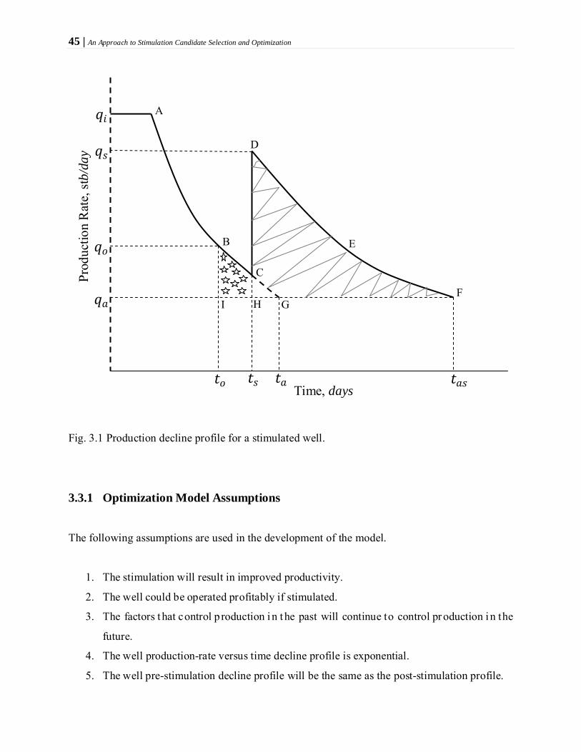
45 | An Approach to Stimulation Candidate Selection and Optimization
Fig. 3.1 Production decline profile for a stimulated well.
3.3.1 Optimization Model Assumptions
The following assumptions are used in the development of the model.
1. The stimulation will result in improved productivity.
2. The well could be operated profitably if stimulated.
3. The factors t hat control p roduction i n t he past will continue to control pr oduction i n the
future.
4. The well production-rate versus time decline profile is exponential.
5. The well pre-stimulation decline profile will be the same as the post-stimulation profile.
Time, days
Prod
uctio
n R
ate,
stb/
day
𝑞𝑞𝑖𝑖
𝑞𝑞𝑠𝑠
𝑞𝑞𝑜𝑜
𝑞𝑞𝑚𝑚
𝑓𝑓𝑜𝑜 𝑓𝑓𝑠𝑠 𝑓𝑓𝑚𝑚 𝑓𝑓𝑚𝑚𝑠𝑠
A
B
C
D
F G H I
E

46 | An Approach to Stimulation Candidate Selection and Optimization
6. The n ominal d ecline r ate c onstant 𝐷𝐷 is the s ame f or bo th t he pr e-stimulation and post-
stimulation profile.
7. The abandonment rate of the well is the same for both the p re-stimulation and post-
stimulation profile.
3.3.2 Stimulation Productivity Ratio
The stimulation productivity ratio 𝐹𝐹 is defined as the ratio of the initial (maximum) production
rate obtained a fter stimulation t o t he p roduction r ate a t which t he well w as considered for
stimulation. From Figure 3.1,
𝐹𝐹 = 𝑞𝑞𝑠𝑠𝑞𝑞𝑜𝑜
……………………………………………….…….……….3.29
3.3.3 The Present-Value Discount Factor
The pr esent va lue i nterest factor (𝑃𝑃𝑉𝑉𝐼𝐼𝐹𝐹) for c ontinuous or daily c ompounding i s u sed i n the
following derivations and it is defined as:
𝑃𝑃𝑉𝑉𝐼𝐼𝐹𝐹 = 𝑠𝑠−𝐼𝐼𝑓𝑓 …………………………………………………………..3.30
where 𝐼𝐼 is t he effective i nterest (discount) rate per day, and 𝑓𝑓 is t he t ime period considered in
days.
3.3.4 Defining the Objective Function, 𝑸𝑸𝑫𝑫
The u ltimate g oal o f well stimulation i s to exploit t he r eservoir p rofitably. I n optimizing well
stimulation processes, the measure of effectiveness is the net i ncremental post-stimulation
production subject to the limitations imposed by the system. Therefore an objective function will
be defined to maximize the net post-stimulation production. The objective function is defined as:
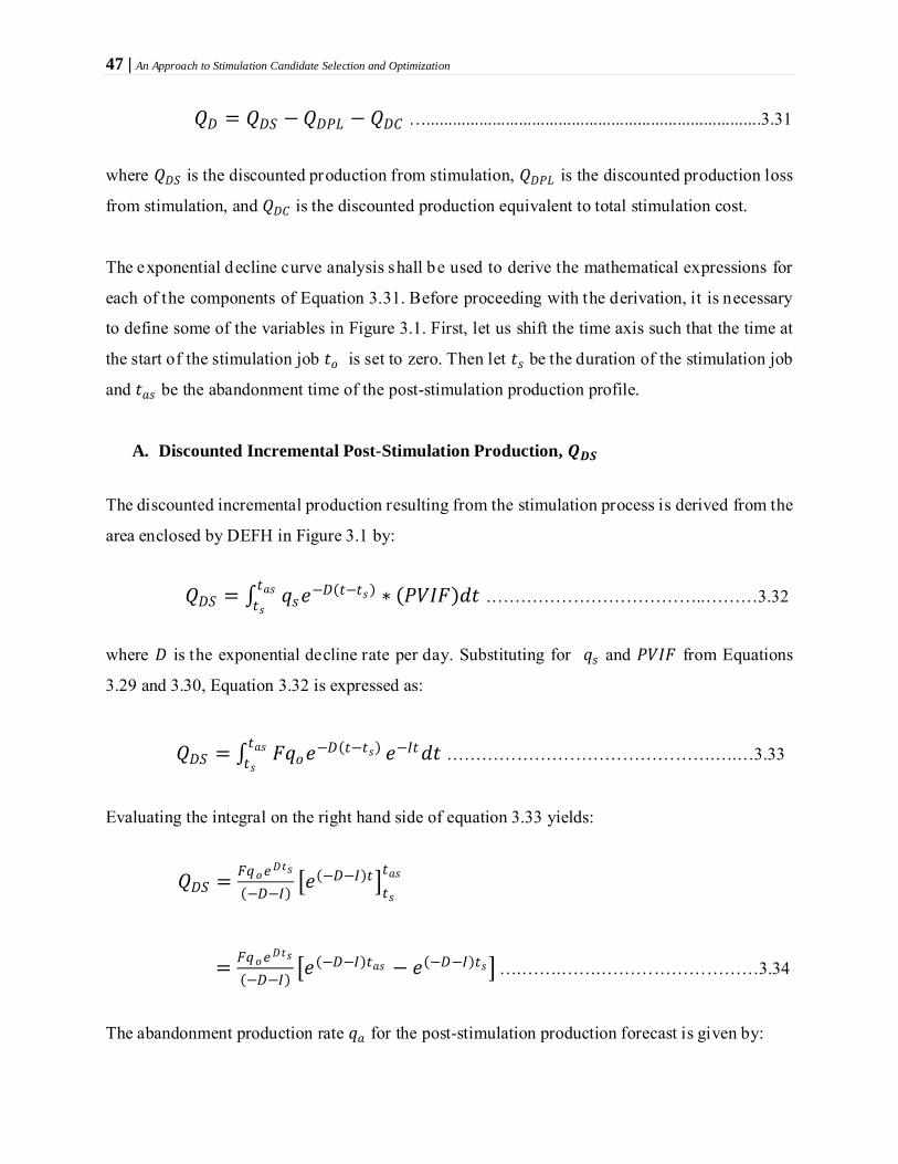
47 | An Approach to Stimulation Candidate Selection and Optimization
𝑄𝑄𝐷𝐷 = 𝑄𝑄𝐷𝐷𝐷𝐷 − 𝑄𝑄𝐷𝐷𝑃𝑃𝐿𝐿 − 𝑄𝑄𝐷𝐷𝐻𝐻 …............................................................................3.31
where 𝑄𝑄𝐷𝐷𝐷𝐷 is the discounted production from stimulation, 𝑄𝑄𝐷𝐷𝑃𝑃𝐿𝐿 is the discounted production loss
from stimulation, and 𝑄𝑄𝐷𝐷𝐻𝐻 is the discounted production equivalent to total stimulation cost.
The exponential decline curve analysis shall be used to derive the mathematical expressions for
each of the components of Equation 3.31. Before proceeding with the derivation, it is necessary
to define some of the variables in Figure 3.1. First, let us shift the time axis such that the time at
the start of the stimulation job 𝑓𝑓𝑜𝑜 is set to zero. Then let 𝑓𝑓𝑠𝑠 be the duration of the stimulation job
and 𝑓𝑓𝑚𝑚𝑠𝑠 be the abandonment time of the post-stimulation production profile.
A. Discounted Incremental Post-Stimulation Production, 𝑸𝑸𝑫𝑫𝑫𝑫
The discounted incremental production resulting from the stimulation process is derived from the
area enclosed by DEFH in Figure 3.1 by:
𝑄𝑄𝐷𝐷𝐷𝐷 = ∫ 𝑞𝑞𝑠𝑠𝑠𝑠−𝐷𝐷(𝑓𝑓−𝑓𝑓𝑠𝑠)𝑓𝑓𝑚𝑚𝑠𝑠𝑓𝑓𝑠𝑠
∗ (𝑃𝑃𝑉𝑉𝐼𝐼𝐹𝐹)𝑑𝑑𝑓𝑓 ………………………………..………3.32
where 𝐷𝐷 is the exponential decline rate per day. Substituting for 𝑞𝑞𝑠𝑠 and 𝑃𝑃𝑉𝑉𝐼𝐼𝐹𝐹 from Equations
3.29 and 3.30, Equation 3.32 is expressed as:
𝑄𝑄𝐷𝐷𝐷𝐷 = ∫ 𝐹𝐹𝑞𝑞𝑜𝑜𝑠𝑠−𝐷𝐷(𝑓𝑓−𝑓𝑓𝑠𝑠)𝑓𝑓𝑚𝑚𝑠𝑠𝑓𝑓𝑠𝑠
𝑠𝑠−𝐼𝐼𝑓𝑓𝑑𝑑𝑓𝑓 ……………………………………….….…3.33
Evaluating the integral on the right hand side of equation 3.33 yields:
𝑄𝑄𝐷𝐷𝐷𝐷 = 𝐹𝐹𝑞𝑞𝑜𝑜𝑠𝑠𝐷𝐷𝑓𝑓𝑠𝑠
(−𝐷𝐷−𝐼𝐼)�𝑠𝑠(−𝐷𝐷−𝐼𝐼)𝑓𝑓 �𝑓𝑓𝑠𝑠
𝑓𝑓𝑚𝑚𝑠𝑠
= 𝐹𝐹𝑞𝑞𝑜𝑜𝑠𝑠𝐷𝐷𝑓𝑓𝑠𝑠
(−𝐷𝐷−𝐼𝐼)�𝑠𝑠(−𝐷𝐷−𝐼𝐼)𝑓𝑓𝑚𝑚𝑠𝑠 − 𝑠𝑠(−𝐷𝐷−𝐼𝐼)𝑓𝑓𝑠𝑠 � ….…….…….………………………3.34
The abandonment production rate 𝑞𝑞𝑚𝑚 for the post-stimulation production forecast is given by:
48 | An Approach to Stimulation Candidate Selection and Optimization
𝑞𝑞𝑚𝑚 = 𝑞𝑞𝑠𝑠𝑠𝑠−𝐷𝐷(𝑓𝑓𝑚𝑚𝑠𝑠−𝑓𝑓𝑠𝑠) …………………………………………………………….3.35
Substituting for 𝑞𝑞𝑠𝑠 from E quation 3. 29 and r earranging Equation 3 .35, the economic l ife
resulting from the stimulation treatment 𝑓𝑓𝑚𝑚𝑠𝑠 can be expressed as:
𝑓𝑓𝑚𝑚𝑠𝑠 = − 1𝐷𝐷𝑙𝑙𝑙𝑙 � 𝑞𝑞𝑚𝑚
𝐹𝐹𝑞𝑞𝑜𝑜�+ 𝑓𝑓𝑠𝑠
= 1𝐷𝐷𝑙𝑙𝑙𝑙𝐹𝐹 − 1
𝐷𝐷𝑙𝑙𝑙𝑙 �𝑞𝑞𝑚𝑚
𝑞𝑞𝑜𝑜�+ 𝑓𝑓𝑠𝑠 ………………………………………….……3.36
Putting Equation 3.36 into 3.34 gives:
𝑄𝑄𝐷𝐷𝐷𝐷 = 𝐹𝐹𝑞𝑞𝑜𝑜𝑠𝑠𝐷𝐷𝑓𝑓𝑠𝑠
(−𝐷𝐷−𝐼𝐼)�𝑠𝑠�
(−𝐷𝐷−𝐼𝐼)𝐷𝐷 𝑙𝑙𝑙𝑙�𝐹𝐹𝑞𝑞𝑜𝑜𝑞𝑞𝑚𝑚
�+(−𝐷𝐷−𝐼𝐼)𝑓𝑓𝑠𝑠� − 𝑠𝑠(−𝐷𝐷−𝐼𝐼)𝑓𝑓𝑠𝑠 � …………………..3.37
Using mathematical i ndices t ransformation of t he f orm: 𝑠𝑠𝑚𝑚+𝑦𝑦 − 𝑠𝑠𝑦𝑦 = 𝑠𝑠𝑦𝑦(𝑠𝑠𝑚𝑚 − 1) and
rearranging the terms, Equation 3.37 can be written as:
𝑄𝑄𝐷𝐷𝐷𝐷 = 𝐹𝐹𝑞𝑞𝑜𝑜𝑠𝑠𝐷𝐷𝑓𝑓𝑠𝑠∗𝑠𝑠(−𝐷𝐷−𝐼𝐼)𝑓𝑓𝑠𝑠
(−𝐷𝐷−𝐼𝐼)�𝐹𝐹�
−𝐷𝐷−𝐼𝐼𝐷𝐷 � �𝑞𝑞𝑚𝑚
𝑞𝑞𝑜𝑜�𝐷𝐷+𝐼𝐼𝐷𝐷 − 1�
= 𝐹𝐹−𝐼𝐼𝐷𝐷 𝑞𝑞𝑜𝑜𝑠𝑠𝐷𝐷𝑓𝑓𝑠𝑠∗𝑠𝑠 (−𝐷𝐷−𝐼𝐼)𝑓𝑓𝑠𝑠
(−𝐷𝐷−𝐼𝐼)�𝑞𝑞𝑚𝑚𝑞𝑞𝑜𝑜�𝐷𝐷+𝐼𝐼𝐷𝐷 − 𝐹𝐹𝑞𝑞𝑜𝑜𝑠𝑠𝐷𝐷𝑓𝑓𝑠𝑠∗𝑠𝑠 (−𝐷𝐷−𝐼𝐼)𝑓𝑓𝑠𝑠
(−𝐷𝐷−𝐼𝐼) ……………….…3.38
B. Discounted Production Loss Due to Stimulation, 𝑸𝑸𝑫𝑫𝑫𝑫𝑫𝑫
The concept of production loss is similar to the idea of opportunity cost. The production loss is
an essential component of the ob jective f unction that t akes care of the z ero-production time
during stimulation.
49 | An Approach to Stimulation Candidate Selection and Optimization
The discounted production loss during the stimulation pr ocess is derived from the area enclosed
by BCHI in Figure 3.1 by:
𝑄𝑄𝐷𝐷𝑃𝑃𝐿𝐿 = ∫ 𝑞𝑞𝑜𝑜𝑠𝑠−𝐷𝐷𝑓𝑓𝑓𝑓𝑠𝑠
0 ∗ (𝑃𝑃𝑉𝑉𝐼𝐼𝐹𝐹)𝑑𝑑𝑓𝑓
= ∫ 𝑞𝑞𝑜𝑜𝑠𝑠−𝐷𝐷𝑓𝑓𝑓𝑓𝑠𝑠
0 𝑠𝑠−𝐼𝐼𝑓𝑓𝑑𝑑𝑓𝑓 ………………………………………………….3.39
Evaluating the integral gives:
𝑄𝑄𝐷𝐷𝑃𝑃𝐿𝐿 = 𝑞𝑞𝑜𝑜(−𝐷𝐷−𝐼𝐼)
�𝑠𝑠(−𝐷𝐷−𝐼𝐼)𝑓𝑓 �0𝑓𝑓𝑠𝑠
= 𝑞𝑞𝑜𝑜(−𝐷𝐷−𝐼𝐼)
�𝑠𝑠(−𝐷𝐷−𝐼𝐼)𝑓𝑓𝑠𝑠 − 1� …………………………………………..…3.40
C. Discounted Stimulation Cost, 𝑸𝑸𝑫𝑫𝑫𝑫
The t otal stimulation c ost, which includes site preparation cost, equipment mobilization &
demobilization cost a nd the stimulation tr eatment cost, can be c onverted to i ts e quivalent
discounted production as:
𝑄𝑄𝐷𝐷𝐻𝐻 = 𝐻𝐻𝑃𝑃∗ 𝑠𝑠−𝐼𝐼𝑓𝑓𝑠𝑠 ….......................................................................................3.41
where 𝐻𝐻 is the total cost of the stimulation treatment in dollars, and 𝑃𝑃 is the price (in dollars) per
barrel of oil.
Substituting Equations 3.38, 3.40 and 3.41 into 3.31 gives:
𝑄𝑄𝐷𝐷 =𝐹𝐹�
−𝐼𝐼𝐷𝐷 �𝑞𝑞𝑜𝑜𝑠𝑠𝐷𝐷𝑓𝑓𝑠𝑠∗𝑠𝑠 (−𝐷𝐷−𝐼𝐼)𝑓𝑓𝑠𝑠
(−𝐷𝐷−𝐼𝐼)�𝑞𝑞𝑚𝑚𝑞𝑞𝑜𝑜��1−�−𝐼𝐼𝐷𝐷 �� − 𝐹𝐹𝑞𝑞𝑜𝑜𝑠𝑠𝐷𝐷𝑓𝑓𝑠𝑠∗𝑠𝑠 (−𝐷𝐷−𝐼𝐼)𝑓𝑓𝑠𝑠
(−𝐷𝐷−𝐼𝐼)

50 | An Approach to Stimulation Candidate Selection and Optimization
− 𝑞𝑞𝑜𝑜(−𝐷𝐷−𝐼𝐼)
�𝑠𝑠(−𝐷𝐷−𝐼𝐼)𝑓𝑓𝑠𝑠 − 1� −𝐻𝐻𝑃𝑃∗ 𝑠𝑠−𝐼𝐼𝑓𝑓𝑠𝑠 …………...……3.42
Let
𝑙𝑙 = −𝐼𝐼𝐷𝐷
………………………………………………………………………….3.43
𝛼𝛼1 = 𝑞𝑞𝑜𝑜(−𝐷𝐷−𝐼𝐼)
…………………………………………………………………….3.44
𝛼𝛼2 = 𝑠𝑠𝐷𝐷𝑓𝑓𝑠𝑠 ………………………………………………………………………3.45
𝛼𝛼3 = 𝑠𝑠(−𝐷𝐷−𝐼𝐼)𝑓𝑓𝑠𝑠 ………………………………………………………………...3.46
𝛼𝛼4 = 𝑠𝑠−𝐼𝐼𝑓𝑓𝑠𝑠
𝑃𝑃 …………………………………………………..……………….…3.47
𝛼𝛼5 = �𝑞𝑞𝑚𝑚𝑞𝑞𝑜𝑜�
(1−𝑙𝑙) ……………………………………………………………......3.48
Therefore the objective function as defined in Equation 3.42 can be expressed in the form:
𝑄𝑄𝐷𝐷 = 𝛼𝛼1𝛼𝛼2𝛼𝛼3𝛼𝛼5𝐹𝐹𝑙𝑙 − 𝛼𝛼1𝛼𝛼2𝛼𝛼3𝐹𝐹− 𝛼𝛼4𝐻𝐻− 𝛼𝛼1(𝛼𝛼3 − 1) ………………………….3.49
3.4 Optimization Model Constraints
To o btain a p ractical s olution t o t he ob jective function, t he f ormulation m ust i nclude some
constraints. In this study, a budgetary constraint is imposed such that the cost of the stimulation
does not exceed the budget as determined by top management. Also, a break-even condition is
imposed such t hat t he r evenue obtained from the stimulation is a t least equal to the stimulation
cost. The reservoir sets a limit on the maximum cumulative production. Existing facilities, both

51 | An Approach to Stimulation Candidate Selection and Optimization
in the sub-surface and surface, limit production rates that can be obtained from the choice of the
stimulation treatment. These constraints are developed mathematically below.
3.4.1 Constraint 1: Break-even Requirement
The discounted revenue from any stimulation decision should be greater than or at least equal to
the discounted cost of the project. That is:
𝑄𝑄𝐷𝐷𝐷𝐷 ≥ 𝑄𝑄𝐷𝐷𝑃𝑃𝐿𝐿 + 𝑄𝑄𝐷𝐷𝐻𝐻 ………………………………………..…3.50
Using the definitions of Equations 3.33, 3.39 and 3.41; Equation 3.50 can be expressed as:
∫ 𝐹𝐹𝑞𝑞𝑜𝑜𝑠𝑠−𝐷𝐷(𝑓𝑓−𝑓𝑓𝑠𝑠)𝑓𝑓𝑚𝑚𝑠𝑠𝑓𝑓𝑠𝑠
𝑠𝑠−𝐼𝐼𝑓𝑓𝑑𝑑𝑓𝑓 ≥ 𝐻𝐻𝑃𝑃∗ 𝑠𝑠−𝐼𝐼𝑓𝑓𝑠𝑠 + ∫ 𝑞𝑞𝑜𝑜𝑠𝑠−𝐷𝐷𝑓𝑓
𝑓𝑓𝑠𝑠0 𝑠𝑠−𝐼𝐼𝑓𝑓𝑑𝑑𝑓𝑓 ……………..…3.51
By examining Equations 3.42 through 3.49, this constraint can be expressed as:
𝛼𝛼1𝛼𝛼2𝛼𝛼3𝛼𝛼5𝐹𝐹𝑙𝑙 − 𝛼𝛼1𝛼𝛼2𝛼𝛼3𝐹𝐹 ≥ 𝛼𝛼4𝐻𝐻 + 𝛼𝛼1(𝛼𝛼3 − 1) …………………….……....3.52
In a practical sense, this constraint is satisfied if and only if the value of the objective function
𝑄𝑄𝐷𝐷 is positive, that is:
𝑄𝑄𝐷𝐷 ≥ 0 ……………………………………………..…3.53
3.4.2 Constraint 2: Remaining Reserve Limitation
The recovery from the stimulation should not e xceed the r emaining produceable oil i n pl ace
(reserve). Mathematically, this constraint can be expressed as:
∫ 𝐹𝐹𝑞𝑞𝑜𝑜𝑠𝑠−𝐷𝐷(𝑓𝑓−𝑓𝑓𝑠𝑠)𝑓𝑓𝑚𝑚𝑠𝑠𝑓𝑓𝑠𝑠
𝑑𝑑𝑓𝑓 ≤ 𝑅𝑅𝑂𝑂𝐼𝐼𝑃𝑃 …………………………………….3.54
52 | An Approach to Stimulation Candidate Selection and Optimization
where 𝑅𝑅𝑂𝑂𝐼𝐼𝑃𝑃 is the remaining oil reserve in place during stimulation. Solving Equation 3.54 we
get:
𝐹𝐹𝑞𝑞𝑜𝑜𝑠𝑠𝐷𝐷𝑓𝑓𝑠𝑠
−𝐷𝐷[𝑠𝑠−𝐷𝐷𝑓𝑓𝑚𝑚𝑠𝑠 − 𝑠𝑠−𝐷𝐷𝑓𝑓𝑠𝑠 ] ≤ 𝑅𝑅𝑂𝑂𝐼𝐼𝑃𝑃 …………………………………3.55
Applying the definition of 𝑓𝑓𝑚𝑚𝑠𝑠 given in Equation 3.36 to Equation 3.55 gives:
𝐹𝐹𝑞𝑞𝑜𝑜𝑠𝑠𝐷𝐷𝑓𝑓𝑠𝑠
−𝐷𝐷�𝑠𝑠−𝐷𝐷�
1𝐷𝐷𝑙𝑙𝑙𝑙�
𝐹𝐹𝑞𝑞𝑜𝑜𝑞𝑞𝑚𝑚
�+𝑓𝑓𝑠𝑠� − 𝑠𝑠−𝐷𝐷𝑓𝑓𝑠𝑠� ≤ 𝑅𝑅𝑂𝑂𝐼𝐼𝑃𝑃 …………………………....3.56
Simplifying,
𝐹𝐹𝑞𝑞𝑜𝑜𝐷𝐷− 𝑞𝑞𝑚𝑚
𝐷𝐷≤ 𝑅𝑅𝑂𝑂𝐼𝐼𝑃𝑃 ………………………………………….…....…3.57
Let
∅1 = 𝑞𝑞𝑜𝑜𝐷𝐷
………………………………………………………..….….3.58
∅2 = 𝑞𝑞𝑚𝑚𝐷𝐷
…………………………….……………………………...…3.59
Substituting Equations 3.58 and 3.59 into 3.57, this constraint can be written as:
∅1𝐹𝐹 − ∅2 ≤ 𝑅𝑅𝑂𝑂𝐼𝐼𝑃𝑃 ………………………………………………...3.60
3.4.3 Constraint 3: Flow String Capacity
The pr oduction r ate a fter s timulation should n ot e xceed t he maximum d esign capacity o f t he
flow string. In the case of gas wells, this constraint is imposed by the gas pipeline capacity.
53 | An Approach to Stimulation Candidate Selection and Optimization
The exponential decline equation for the post-stimulation production rate 𝑞𝑞𝑓𝑓 can be expressed as:
𝑞𝑞𝑓𝑓 = 𝑞𝑞𝑠𝑠𝑠𝑠−𝐷𝐷(𝑓𝑓−𝑓𝑓𝑠𝑠)
= 𝐹𝐹𝑞𝑞𝑜𝑜𝑠𝑠−𝐷𝐷(𝑓𝑓−𝑓𝑓𝑠𝑠) ………………………………………………..3.61
The m aximum production rate is obtained w hen the well is opened f or production just after
stimulation, i.e. at time 𝑓𝑓 = 𝑓𝑓𝑠𝑠 (see Fig. 3.1). Using this substitution in Equation 3.61, constraint
3 can then be formulated as:
𝐹𝐹𝑞𝑞𝑜𝑜 ≤ 𝑞𝑞𝑚𝑚𝑚𝑚𝑚𝑚 therefore:
𝐹𝐹 ≤ 𝑞𝑞𝑚𝑚𝑚𝑚𝑚𝑚𝑞𝑞𝑜𝑜
…….…………………………………………………...3.62
where 𝑞𝑞𝑚𝑚𝑚𝑚𝑚𝑚 is the maximum design capacity (flow rate) for the well tubing string.
3.4.4 Constraint 4: Budget Allocation
The total cost of s timulation should not exceed the maximum budget allocated by management
for the job. This constraint is formulated mathematically as:
𝐻𝐻 ≤ 𝐻𝐻𝑚𝑚𝑚𝑚𝑚𝑚 ……………………………..………………………3.63
where 𝐻𝐻𝑚𝑚𝑚𝑚𝑚𝑚 is the maximum budget allocated by management for stimulation.
3.4.5 Constraint 5: Maximum Formation Productivity Ratio
Given a s et of r eservoir a nd t reatment pa rameters, t he r eservoir c ould o nly be stimulated t o a
certain maximum extent.
54 | An Approach to Stimulation Candidate Selection and Optimization
𝐹𝐹 ≤ 𝐹𝐹𝑚𝑚𝑚𝑚𝑚𝑚 ………………………………………………………3.64
where 𝐹𝐹𝑚𝑚𝑚𝑚𝑚𝑚 is the m aximum productivity ratio t hat c an be o btained given the reservoir a nd
treatment pa rameters. I t i s t he productivity ratio obtained from t he d esign module pr esented i n
section 3.2.1 through 3.2.3.
3.4.6 Constraint 6: Productivity Improvement
The stimulation must, at l east, result i n a n i mprovement i n t he productivity r atio and must not
itself cause m ore damage to the formation. This constraint is imposed on the productivity ratio
such that it must not be less than one or negative. It can be formulated mathematically as:
𝐹𝐹 ≥ 1 ………………………….…………………………………3.65
3.5 Stimulation Cost & Productivity Ratio Relationship
From t he design module pr esented i n section 3 .21 t hrough 3.23, i t c ould be observed t hat t he
input design parameters determine the stimulation cost (C) a nd t he maximum pr oductivity ratio
(F). For e xample, f rom the acidizing d esign m odule in s ection 3.21, it c ould b e seen that t he
stimulation c ost depends on t he vo lume of acid pumped, and also the volume of a cid pumped
will d etermine t he extent o f damage r emoval ( productivity r atio). T his discussion shows t hat a
relationship can be formulated between the stimulation cost and the productivity ratio based on
the design module. Hence, in order to use the model presented in section 3 .3 as an optimization
model, i t i s necessary t o develop a stimulation cost versus productivity ratio r elationship ba sed
on the design module presented.
The combined effects of the treatment and reservoir variables are lumped into a stimulation cost
versus productivity equation of the form:
𝐻𝐻 = 𝑚𝑚𝐹𝐹𝑜𝑜 ……………………………….…………………..3.66

55 | An Approach to Stimulation Candidate Selection and Optimization
where 𝑚𝑚 and 𝑜𝑜 are obtained from the power equation of the trend l ine of a log-log plot of
stimulation cost v ersus p roductivity r atio. It is this equation that in corporates the stimulation
option into the optimization model. Hence we must substitute Equation 3.66 into Equation 3.49
in order to use the model.
3.6 Summary of the Optimization Model
Combining the objective function and the constraints, the optimization model formulated can be
summarized as:
Maximize:
𝑄𝑄𝐷𝐷 = 𝛼𝛼1𝛼𝛼2𝛼𝛼3𝛼𝛼5𝐹𝐹𝑙𝑙 −𝛼𝛼1𝛼𝛼2𝛼𝛼3𝐹𝐹−𝛼𝛼4 ∗ 𝑚𝑚𝐹𝐹𝑜𝑜 − 𝛼𝛼1(𝛼𝛼3 − 1) …………………….3.49
subject to:
1. Break-even Requirement:
𝛼𝛼1𝛼𝛼2𝛼𝛼3𝛼𝛼5𝐹𝐹𝑙𝑙 − 𝛼𝛼1𝛼𝛼2𝛼𝛼3𝐹𝐹 ≥ 𝛼𝛼4 ∗ 𝑚𝑚𝐹𝐹𝑜𝑜 + 𝛼𝛼1(𝛼𝛼3 − 1) ……………………....3.52
2. Remaining Reserve Limitation:
∅1𝐹𝐹 − ∅2 ≤ 𝑅𝑅𝑂𝑂𝐼𝐼𝑃𝑃 ………………………………………………...3.60
3. Flow String Capacity:
𝐹𝐹 ≤ 𝑞𝑞𝑚𝑚𝑚𝑚𝑚𝑚𝑞𝑞𝑜𝑜
…….…………….………………………………….3.62
4. Budget Allocation:
𝐻𝐻 ≤ 𝐻𝐻𝑚𝑚𝑚𝑚𝑚𝑚 ……………………………..………………….……3.63
5. Maximum Formation Productivity Ratio:
𝐹𝐹 ≤ 𝐹𝐹𝐹𝐹 …………………………………………………….……3.64
56 | An Approach to Stimulation Candidate Selection and Optimization
6. Productivity Improvement:
𝐹𝐹 ≥ 1 ……………………….………………………………..…3.65
The constants 𝑙𝑙, 𝛼𝛼1 , 𝛼𝛼2, 𝛼𝛼3, 𝛼𝛼4 and 𝛼𝛼5 are as defined in Equation 3.43 through 3 .48; ∅1 and ∅2
are defined in Equation 3.58 and 3.59; 𝑚𝑚 and 𝑜𝑜 are from Equation 3.66.
It is important to note that the optimization model is a non-linear programming (NLP) problem.
The o bjective function consists o f t wo variables, na mely productivity r atio 𝐹𝐹 and total
stimulation cost 𝐻𝐻. The two variables are related based on the discussion presented in section 3.5.
This research investigated the matrix stimulation cost and performance data presented by Vogt et
al.88
An a ttempt was ma de to obtain a relationship between total stimulation cost 𝐻𝐻 and
productivity ratio 𝐹𝐹. The data is presented in Table 1 of Appendix B. A regression analysis on the
data using Microsoft Excel shows a trend between pr oductivity r atio a nd t otal stimulation c ost
similar to the form presented in Equation 3.66. Therefore, to use this model, the stimulation cost
versus productivity ratio constants 𝑚𝑚 and 𝑜𝑜 must be obtained from the design module. The design
and op timization m odel included i n t he a ccompany compact di sk ( CD) of t his t hesis only
requires the input, stimulation design parameters, to generate the constants.
3.7 Solution to the Optimization Model
In this research, the model was solved using the Solver in Microsoft Excel and also What’s Best
10.0 LINDO S ystems optimization so ftware. The r esults obtained w ere v erified b y c omparing
the solution with t hat ob tained by us ing Mathematica 7.0 – software developed by Wolfram
Research. The Solver i mplemented i n E xcel ( developed by Frontline Systems) u ses numerical
iterative methods (generalized reduced gr adient m ethod) to s olve e quations a nd t o o ptimize
linear and n onlinear functions with e ither c ontinuous or i nteger variables. But Solver has some
limitations hence t he need t o verify t he r esults. Wolfram’s Mathematica 7.0 on t he ot her ha nd
uses several numerical algorithms for constrained no nlinear optimization. T he a lgorithms ar e
categorized into gradient-based methods and direct search methods. Gradient-based methods use
first d erivatives ( gradients) or second d erivatives ( Hessians). Examples a re t he sequential
57 | An Approach to Stimulation Candidate Selection and Optimization
quadratic programming ( SQP) m ethod, t he a ugmented Lagrangian method, a nd t he ( nonlinear)
interior point method. D irect search methods do no t us e derivative i nformation. E xamples a re
Nelder Mead, genetic algorithm and d ifferential e volution, and s imulated a nnealing. The most
general m ethod used b y Mathematica 7.0 for e xact c onstrained op timization problems is based
on the cylindrical algebraic decomposition (CAD) algorithm. Mathematica 7.0 can automatically
choose a lgorithm based on t he nature o f t he problem - a quality which makes i t the preferred
choice for verification of the Solver’s results.
Based on the stimulation modules presented in this chapter, a computer model is developed using
Microsoft Excel. This model is intended for use in the Niger Delta and as such it is assumed that
all w ells can either be acidized, g ravel-packed or r e-completed. T he screening module i s n ot
included in the computer model because it is assumed that prior to the use of this model, the well
must have been matched with one of acidizing, gravel-packing or re-completion. Also, hydraulic
fracturing is not considered in this m odel because t he N iger D elta formation is made up o f
sandstone with good permeability.

58 | An Approach to Stimulation Candidate Selection and Optimization
Chapter Four
Model Validation, Results and Discussion
To s tudy t he b ehavior o f t he o ptimization model t o changes i n i nput parameters, a s ensitivity
analysis was carried out on the acidizing model. Some published data from the Niger Delta were
also used to validate the model. The results obtained are discussed in the following section.
4.1 Sensitivity Analysis
The parameters i n t he following section were va ried a nd the values of t he o ptimal objective
function obtained are plotted against the productivity ratio f or each parameter va lue. The input
data used for the sensitivity analysis are presented in Table 4.1.
4.1.1 Effect of Price of Oil
The p rice o f o il d etermines the amount of revenue derived from the s timulation. T herefore an
increase in the price of oil is accompanied with an increase in the optimal point of the objective
function as shown in Fig. 4.1. The price of oil is purely an economic input to the optimization
model. T he decision t o perform well s timulation depends on t he current price o f oil. H ence t he
higher t he p rice of oil, t he greater t he benefit derived from s timulation. It is important to note
that below a pr oductivity ratio o f about 3 .2, the di scounted pr oduction will not change with the
price of oil, but the overall monetary benefit will reduce when the price of oil falls.
4.1.2 Effect of Discount Rate
Fig. 4.2 illustrates the effect of the interest rate on t he objective f unction. The value of t he
discount rate was varied from 5% to 20%. The discounted production decreases with an increase
in t he discount r ate. The di scount rate can be viewed a s an additional cost of stimulation. The
higher the discount rate, the higher the cost of money and well stimulation, and consequently, the
lower the benefit to be derived from the stimulation job.
4.1.3 Effect of Decline Rate
The effect of the exponential decline rate on the objective function is shown in Fig. 4.3. For this
analysis, the value of the decline constant was varied between 0.032/yr and 0.32/yr. It is noticed
that the smaller the exponential decline rate, the higher the stimulation benefit. The exponential

59 | An Approach to Stimulation Candidate Selection and Optimization
Table 4.1 Input Data for Sensitivity Analysis
Average Reservoir Pressure, Pr 2200 psi Drainage Radius, r 1053 ft e Wellbore Radius, r 0.3 ft w Net Pay Thickness, h 20 ft Depth of Formation 12000 ft Damaged Zone Radius r 7 ft d Undamaged Reservoir Permeability, k 200 md Damaged Zone Permeability, k 20 md d
Porosity 25% Formation Volume Factor 1 bbl/stb Acid Hydrostatic Gradient 0.45 psi/ft Specific Gravity of Acid 1.04 Viscosity of Injected Acid 0.57 cp Pump Rate 2 bbl/min
Safe Margin for Injection Pressure 200 psi Diameter of Coil Tubing 1.75 inches Cost of Acid Per Unit Volume $ 38 per gal
𝛼𝛼 0.4 psi/ft Current Production Rate, q 1000 stb/d o Abandonment Rate, q 200 stb/d a
Exponential Decline Rate, D 0.32 per day Duration of Stimulation, t 2 days s Remaining Recoverable Reserve, ROIP 3 MM stb Price Per Barrel of Oil, P 80 $/stb Effective Discount Rate Per Day, I 10% Tubing Maximum Design Flowrate, q 10000 stb/d max
Maximum Stimulation Budget, C 1.2 MM $ max
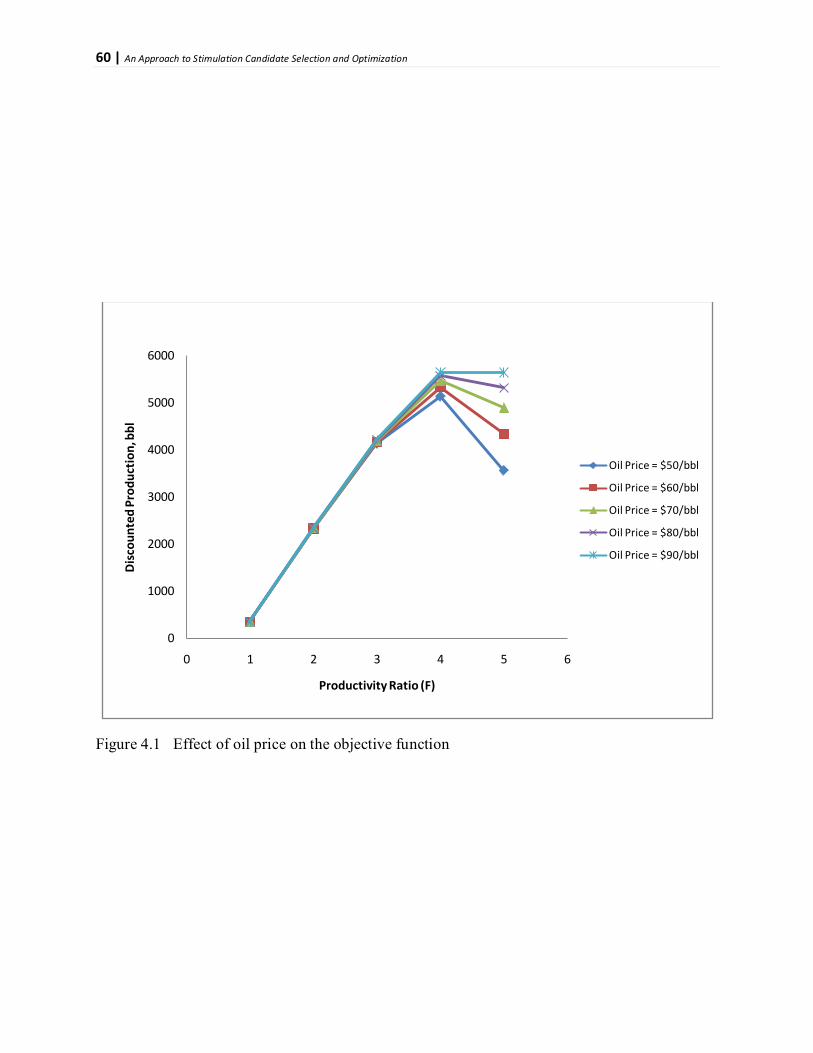
60 | An Approach to Stimulation Candidate Selection and Optimization
Figure 4.1 Effect of oil price on the objective function
0
1000
2000
3000
4000
5000
6000
0 1 2 3 4 5 6
Dis
coun
ted
Prod
uctio
n, b
bl
Productivity Ratio (F)
Oil Price = $50/bbl
Oil Price = $60/bbl
Oil Price = $70/bbl
Oil Price = $80/bbl
Oil Price = $90/bbl

61 | An Approach to Stimulation Candidate Selection and Optimization
Figure 4.2 Effect of discount rate on the objective function
0
1000
2000
3000
4000
5000
6000
7000
8000
0 1 2 3 4 5 6
Dis
coun
ted
Prod
uctio
n, b
bl
Productivity Ratio (F)
I = 5%
I = 10%
I = 15%
I = 20%

62 | An Approach to Stimulation Candidate Selection and Optimization
Figure 4.3 Effect of decline rate on the objective function
0
5000
10000
15000
20000
25000
30000
0 1 2 3 4 5 6 7 8
Dis
coun
ted
Prod
uctio
n, b
bl
Productivity Ratio (F)
D = 0.032/yr
D = 0.16/yr
D = 0.32/yr

63 | An Approach to Stimulation Candidate Selection and Optimization
decline rate is the parameter that controls the concavity of the objective function. The smaller the
value of the exponential decline constant for a w ell pr oduction pr ofile, the more the benefit we
could get if such well i s considered f or s timulation. In pr actice, w e ha ve no c ontrol ov er the
value of the decline rate constant. H owever, i t gives us a direct i nsight i nto candidate selection
for stimulation decisions. Smaller decline rate is desirable for profitable stimulation decisions.
4.1.4 Effect of Pre-Stimulation Production Rate
The effect of pre-stimulation production rate on t he objective function is i llustrated i n F ig. 4 .4.
The value of the pre-stimulation production rate was varied from 500stb/d to 1500stb/d. A higher
pre-stimulation pr oduction r ate indicates a higher r eservoir energy dr ive. T he main goal of
stimulation i s t o i ncrease pr oduction u sing t he r eservoir e nergy a s t he driving force in moving
the oil from th e r eservoir i nto th e wellbore. If t he r eservoir has litt le or n o e nergy, stimulation
benefit w ill b e small. Th is is clearly illustrated in the figure. Since a higher pre-stimulation
production will give a higher optimal point in the objective function, therefore, from the figure, a
higher p re-stimulation production rate will give a higher optimal stimulation benefit. This
suggests that as production declines during production, there should be an optimal time in which
it is best to initial stimulation jobs. Because of the huge impact of this pre-stimulation production
rate on t he ob jective function, this parameter must be given a major attention in the selection of
stimulation candidates
4.1.5 Effect of Abandonment Rate
The e ffect of t he a bandonment r ate o n t he stimulation d ecision i s shown i n F ig. 4. 5. The
abandonment r ate i s v aried b etween 100stb/d a nd 50 0stb/d. I t i s observed t hat i ncreasing t he
abandonment r ate r esults i n decrease i n t he overall s timulation b enefit. The a bandonment r ate
can be i nterpreted in terms of t he r emaining r ecoverable o il i n t he r eservoir. A hi gher
abandonment r ate m eans a h igher a mount of r ecoverable oil r emaining i n t he r eservoir. B ut a
reduced incremental production is expected because when the abandonment rate is set high, the
incremental p roduction w ill be reduced since w e h ave a l imit t o w hich w e ca n produce.
Consequently, a reduced incremental production will eventually decrease the optimal point of the
objective function. Therefore, the abandonment rate is a major factor that influences the choice
of stimulation candidate selection.

64 | An Approach to Stimulation Candidate Selection and Optimization
Figure 4.4 Effect of pre-stimulation production rate on the objective function
0
2000
4000
6000
8000
10000
12000
0 1 2 3 4 5 6
Dis
coun
ted
Prod
uctio
n, b
bl
Productivity Ratio (F)
qo = 500stb/d
qo = 1000stb/d
qo = 1500stb/d
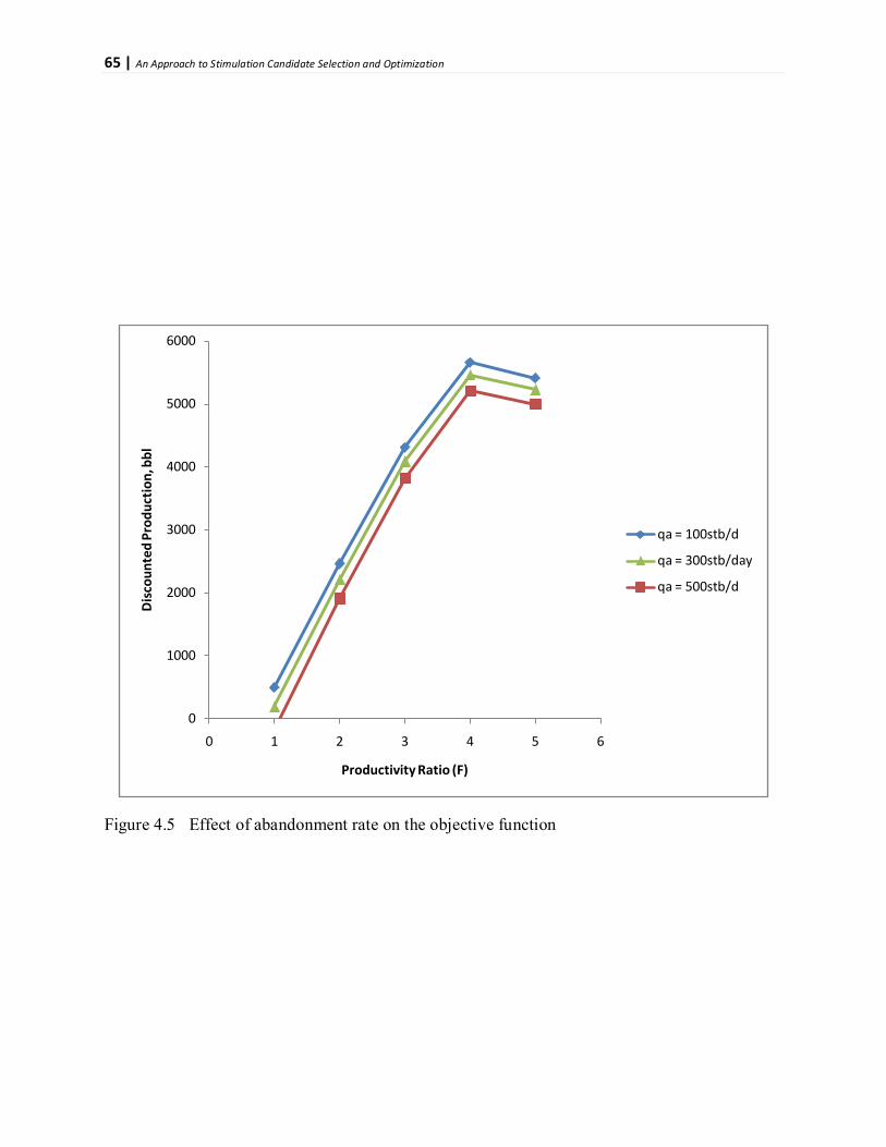
65 | An Approach to Stimulation Candidate Selection and Optimization
Figure 4.5 Effect of abandonment rate on the objective function
0
1000
2000
3000
4000
5000
6000
0 1 2 3 4 5 6
Dis
coun
ted
Prod
uctio
n, b
bl
Productivity Ratio (F)
qa = 100stb/d
qa = 300stb/day
qa = 500stb/d

66 | An Approach to Stimulation Candidate Selection and Optimization
4.1.6 Effect of Stimulation Time
The stimulation time represents the duration of time the stimulation job is performed. The effect
of the s timulation t ime on the optimal point of the objective function is shown in Fig. 4.6. The
stimulation time is varied between 1 day and 3 days. The optimal point of the objective function
lowers as the stimulation time increases. This means that if more time is spent on the stimulation
job, t he p roduction l oss du ring t he du ration of s timulation will i ncrease, a nd hence, l owers t he
overall benefit d erivable f rom the s timulation j ob. Therefore i t i s b eneficial i f t he duration of
stimulation is reduced to possibly a day in order to get a higher return from stimulation.
4.2 Model Validation: Case Study 1
In this section, the optimization model is applied with the acidizing treatment model to quantify
stimulation benefit derivable from four typical acidizing jobs, and also, to rank the wells for the
stimulation process. Production data from four wells: Well BU 1, Well BU 2, Well BU 3 and Well
BU 4 were u sed t o va lidate t he model. The four w ells completed i n May 2004 are l ocated in
Bestfields, offshore Niger Delta. This high permeability field is located in a water depth of 200m.
The a verage pe ak p roduction recorded i n J anuary 2006 from e ach of t he four wells i s
7000stb/day. Production d ecline s tarts a fter a 3 -year peak pr oduction period. The a vailable
production data f or each o f t he four wells shows t hat t he d ecline pr ofile for e ach w ell i s
exponential. The wells are being considered as potential candidates for acidizing after a well test
confirms the presence of acid removable damage. The field data is presented in Table 4.2. These
data served a s input da ta for t he acidizing design a nd optimization model. Additional da ta used
were t aken from published l iteratures by Ofoh a nd H eikal89, Nnanna et al.73, Nnanna an d
Ajienka76, and Onyekonwu80
The data in Table 4.2 are used to formulate the Bestfield Model, which gives an insight into how
the model can be used to optimize acidizing candidate well selection process in the Niger Delta.
The design and optimization model is available in the included CD.
.
4.2.1 Formulation of the Bestfield Model
In combination with the data provided in Table 4.2, let’s assume that the remaining recoverable
reserve is 500 MM bbls, and the tubing maximum design flow rate for each well is 12500stb/d.
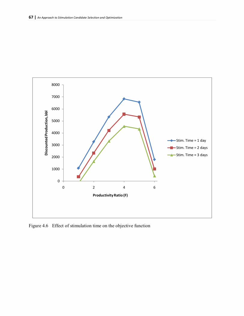
67 | An Approach to Stimulation Candidate Selection and Optimization
Figure 4.6 Effect of stimulation time on the objective function
0
1000
2000
3000
4000
5000
6000
7000
8000
0 2 4 6
Dis
coun
ted
Prod
uctio
n, b
bl
Productivity Ratio (F)
Stim. Time = 1 day
Stim. Time = 2 days
Stim. Time = 3 days
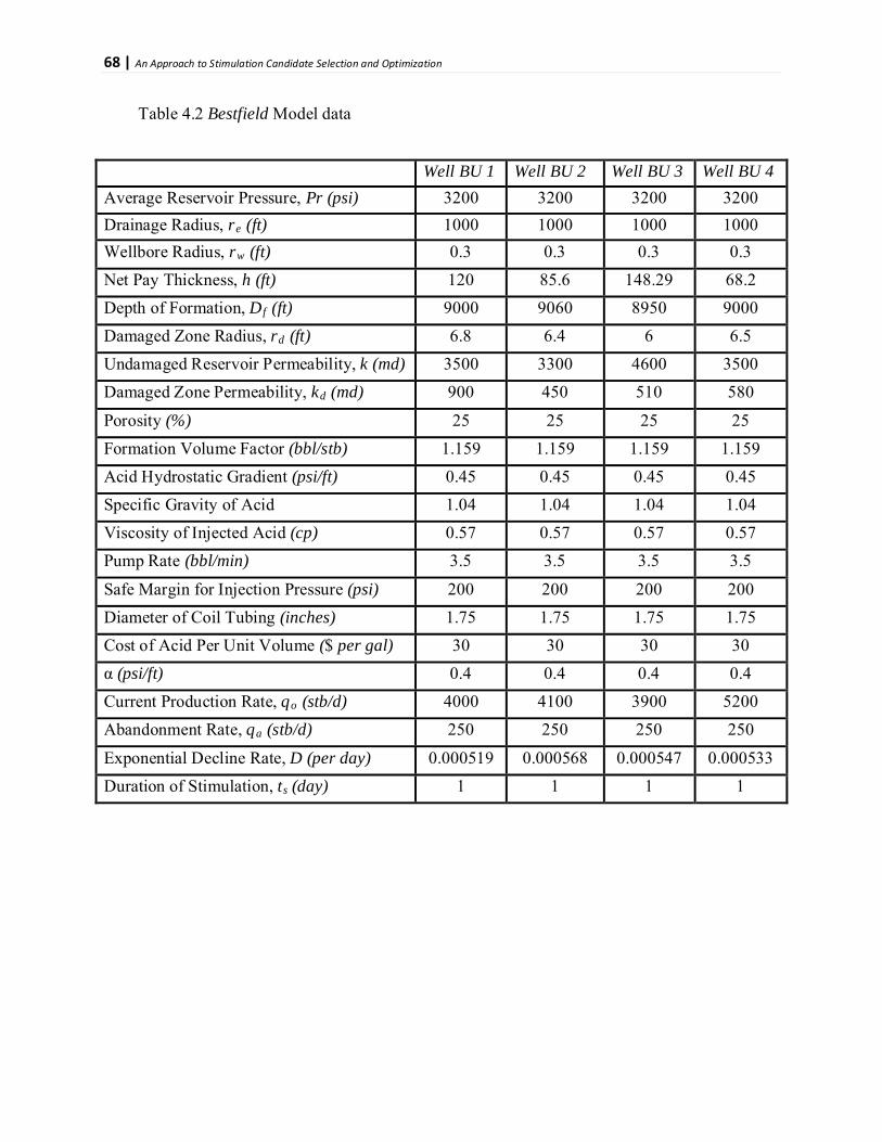
68 | An Approach to Stimulation Candidate Selection and Optimization
Table 4.2 Bestfield Model data
Well BU 1 Well BU 2 Well BU 3 Well BU 4 Average Reservoir Pressure, Pr (psi) 3200 3200 3200 3200 Drainage Radius, re 1000 (ft) 1000 1000 1000 Wellbore Radius, rw 0.3 (ft) 0.3 0.3 0.3 Net Pay Thickness, h (ft) 120 85.6 148.29 68.2 Depth of Formation, Df 9000 (ft) 9060 8950 9000 Damaged Zone Radius, rd 6.8 (ft) 6.4 6 6.5 Undamaged Reservoir Permeability, k (md) 3500 3300 4600 3500 Damaged Zone Permeability, kd 900 (md) 450 510 580
Porosity (%) 25 25 25 25 Formation Volume Factor (bbl/stb) 1.159 1.159 1.159 1.159 Acid Hydrostatic Gradient (psi/ft) 0.45 0.45 0.45 0.45 Specific Gravity of Acid 1.04 1.04 1.04 1.04 Viscosity of Injected Acid (cp) 0.57 0.57 0.57 0.57 Pump Rate (bbl/min) 3.5 3.5 3.5 3.5
Safe Margin for Injection Pressure (psi) 200 200 200 200 Diameter of Coil Tubing (inches) 1.75 1.75 1.75 1.75 Cost of Acid Per Unit Volume ($ per gal) 30 30 30 30 α (psi/ft) 0.4 0.4 0.4 0.4 Current Production Rate, qo 4000 (stb/d) 4100 3900 5200 Abandonment Rate, qa 250 (stb/d) 250 250 250
Exponential Decline Rate, D (per day) 0.000519 0.000568 0.000547 0.000533 Duration of Stimulation, ts 1 (day) 1 1 1

69 | An Approach to Stimulation Candidate Selection and Optimization
Also let’s assume an average oil price of $80/bbl, effective discount rate of 10% and a maximum
acidizing budget of $1200000 per well.
Using these data, the model is formulated as follows:
Step A:
The Cost versus Productivity-Ratio plots for each of the four wells was generated by the design
model. The a nalysis i n t he following section is for Well BU 3. The analysis for t he Well BU 1,
Well BU 2 and Well BU 4 is similar, h ence o nly t he results w ere discussed. T he C ost versus
Productivity-Ratio plot for the Well BU 3 data is shown in Fig. 4.7.
Enter each well data given into the Acidizing Design and Optimization Model and
generate the Cost versus Productivity-Ratio relationship for each well.
Step B:
For the Well BU 3 input data, the equation is obtained as:
Obtain the relationship between the stimulation cost (C) and productivity ratio (F) in
form of power equation of a trendline through a log-log regression of the data.
𝐶𝐶 = 87.15𝐹𝐹6.499 ............…….….……….………..………4.1
The above relationship, as presented in Equation 4.1 was obtained from a regression analysis o f
the simulated data generated by the design model using Microsoft Excel. The design model used
the Well BU 3 input data to account f or c ost as s hown in Equation 4.1 based on t he damaged
radius of the well, which is one of the parameters with greatest influence on the acidizing design.
The acidizing design and optimization model will generate this equation once the data input step
is completed.
Step C:
The constants needed to define the objective function can be calculated easily using the equation
listed a bove. It i s i mportant t o point ou t that w hile u sing the a cidizing a nd d esign model
included in the CD, one does not need to calculate the objective function as presented below. The
program is designed to calculate the objective function, set up the constraints and then awaits the
user t o call a s olver pr ogram f or t he o ptimization step. Hence, S tep C i s only i ncluded for t he
purpose of proper understanding of how the model and its constraints were formulated.
Use Equations 3.49, 3.52, 3.60, 3.62, 3.63, 3.64 & 3.65 to formulate the objective
function and its constraints.

70 | An Approach to Stimulation Candidate Selection and Optimization
The non linear programming model formulated as a maximization problem using the Well BU 3
data is presented below.
𝒎𝒎𝒎𝒎𝒎𝒎𝒎𝒎𝒎𝒎𝒎𝒎𝒛𝒛𝒛𝒛:
𝑄𝑄𝐷𝐷 = −1.7008 × 10−215𝐹𝐹−182.82 + 3.5097 × 10⁴𝐹𝐹
−0.9857𝐹𝐹6.499 − 3710.3427 .................................4.2
𝒔𝒔𝒔𝒔𝒔𝒔𝒔𝒔𝒛𝒛𝒔𝒔𝒔𝒔 𝒔𝒔𝒕𝒕:
1. Break-even Constraint:
−1.7008 × 10−215𝐹𝐹−182.82 + 3.5097 × 10⁴𝐹𝐹
≥ 0.9857𝐹𝐹6.499 + 3710.3427 …….……4.3
2. Remaining Reserve Constraint:
7.1298𝐹𝐹 − 457038.391 ≤ 500000000 …………………………4.4
3. Flow String Capacity Constraint:
𝐹𝐹 ≤ 3.21 ……………………………………………………...4.5
4. Budget Allocation Constraint:
87.15𝐹𝐹6.499 ≤ 1000000 ………………………..…………4.6
5. Productivity Improvement Constraint:
𝐹𝐹 ≥ 1 …………………………………………………………4.7
6. Maximum Formation Productivity Ratio Constraint:
𝐹𝐹 ≤ 4.20 ………………………………………………………4.8
From the non-linear programming optimization problem presented a bove i t could b e seen t hat,
simply, we seek an optimum value for the productivity ratio which has a lower and upper bound
of 1 and 3.21 respectively. This is true because the limit sets by the facility constraints (Equation
4.5) is more binding than the maximum productivity r atio a ttainable given t he r eservoir a nd
treatment parameters (Equation 4.8).
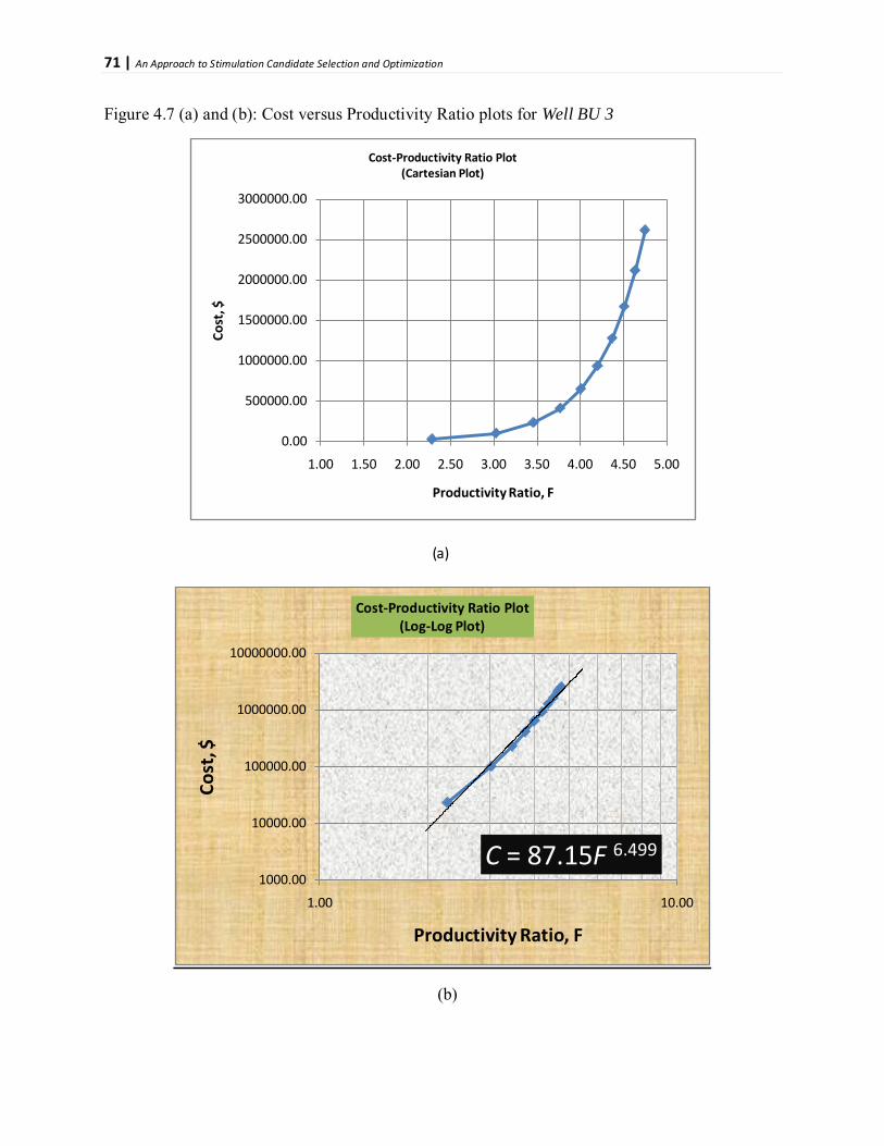
71 | An Approach to Stimulation Candidate Selection and Optimization
Figure 4.7 (a) and (b): Cost versus Productivity Ratio plots for Well BU 3
(a)
(b)
0.00
500000.00
1000000.00
1500000.00
2000000.00
2500000.00
3000000.00
1.00 1.50 2.00 2.50 3.00 3.50 4.00 4.50 5.00
Cost
, $
Productivity Ratio, F
Cost-Productivity Ratio Plot(Cartesian Plot)
C = 87.15F 6.4991000.00
10000.00
100000.00
1000000.00
10000000.00
1.00 10.00
Cost
, $
Productivity Ratio, F
Cost-Productivity Ratio Plot(Log-Log Plot)
72 | An Approach to Stimulation Candidate Selection and Optimization
Step D:
In this research, two different solvers, which use different a lgorithms, were used to get an
optimum solution to the model. The solvers are: Frontline System’s Microsoft Excel Solver and
What’s Best 10.0 LINDO S ystems op timization s oftware. T he solution t o t he model was t hen
verified u sing t he W olfram R esearch’s Mathematica 7.0. The results a re discussed i n t he
following sections.
Find a solution to the non-linear programming model formulated in Step C above.
4.2.2 Solution of the Well BU 3 Model
The Well BU 3 Model was solved u sing t he Microsoft Excel Solver and What’s Best 10.0, the
results a re presented i n Appendix C and D . The solutions gave the same r esult for t he optimal
point.
The value of the objective function at optimal point is:
𝑄𝑄𝐷𝐷 = 106868.12 𝑏𝑏𝑏𝑏𝑏𝑏𝑏𝑏
The v alue o f t he productivity r atio a t th e o ptimal p oint i s g iven a s t he f inal value o f t he
adjustable cell. The optimal productivity ratio is equal to 3.21.
The o bjective function b ehaviour is viewed in the vicinity of the lower and upper bound of its
constraint. Mathematica 7.0 is us ed t o ge nerate t he pl ot shown i n A ppendix E . Also,
Mathematica 7.0 is us ed t o s olve t he non -linear pr ogramming op timization problem. The
functions NMaximize and Maximize are u sed a nd t he r esult for t he objective function i s
107012.6.7 bbls, while the va lue of the pr oductivity ratio at the optimal point is 3.21. The input
syntax for Mathematica 7.0 is also included in Appendix E.
The slight variation i n t he r esults obtained is du e t o t he fact t hat approximated values a re
inputted i nto Mathematica 7.0 for the optimization. Also, Mathematica 7.0 uses the Cylindrical
Algebraic Decomposition algorithm to s eek i ts optimal point while EXCEL o r L INDO solver
uses the conjugate gradient method. This result is only used to know that the solution obtained is
in the correct range. It is important to note that both results are the same when corrected to three
significant figures. The plot in Appendix E gives a better picture of the optimal point.
73 | An Approach to Stimulation Candidate Selection and Optimization
The results obtained using the Microsoft Excel Solver and What’s Best 10.0, is taken as the actual
value of the objective function at the optimal point. Hence, the following discussions are based
on this result.
4.2.3 Discussion of the Well BU 3 Model Result
This optimal v alue of the objective f unction is 106868.12bbls, meaning that i f this well i s
considered for s timulation, given that t he a ssumptions c onsidered i n section 4 .2.1 a re binding,
the benefit derivable is 106868.12bbls of oi l. The l ife of the well is estimated to be 19.6 years.
The payout time on the acidizing cost is also estimated to be 0.94 day.
The A nswer R eport for Well BU 3 in Appendix C, Section 1, shows t hat five o ut of t he six
constraints are not binding. The only binding constraint is the tubing string capacity. Hence, the
optimal solution was f ound within th e lim its o f a ll t he constraints. That is t o s ay th at a ll
constraints are satisfied. No constraint is violated.
The tubing string capacity constraint is binding, meaning that if the tubing f low capacity is
increased, there will be more benefit from this project, but on the other hand, this extremely high
rate w ill kill o ur w ell s ooner than la ter. In g eneral, f or a c onstraint to b e bi nding m eans any
movement to the right would still give a better result to the objective function.
From the sensitivity report it could be seen that the value of the Lagrange Multiplier associated
with th e flow string c apacity c onstraint is 31221.9668. T his gi ves a n i dea of t he fractional
change of the ob jective f unction i f t he flow s tring c apacity c onstraint c hanges b y 1stb/day.
Hence, if the flow string capacity is increased by 1stb/day, the benefit derivable from stimulation
will increase by 31221.9668 bbls. Hence, the v alue o f t he Lagrange Multiplier will help th e
stimulation design engineer to know i f it is necessary to increase the stimulation benefit by
adjusting the constraints. It also gives the estimate of the derivable benefit.
Considering Well BU 1, t he u ltimate s olution obt ained is s hown in A ppendix C, Section 2 . All
constraints are n ot b inding, m eaning that t he optimum po int of the objective f unction w as
attained before any of the constraint bound was reached. Hence any shift to the right or left of the
optimum point will only decrease the stimulation benefit.
74 | An Approach to Stimulation Candidate Selection and Optimization
4.2.4 Application of the Model Result in Candidate Selection
This m odel can be u sed easily t o r ank stimulation candidates based on t he be nefits derivable
from t he stimulation operation and the pa yout t ime. Since the ultimate goal of stimulation is to
increase pr oduction, the well with th e h ighest stimulation benefit and shortest pa yout t ime is
considered f irst for s timulation. Hence wells are ranked first to last in t he decreasing order o f
their s timulation benefits (profits), provided the payout i s a cceptable by management. The w ell
ranked “first” is then selected for stimulation before the one ranked “second” and so on.
The t able below gives a s imple stimulation ca ndidate selection c harts for the four w ells i n
Bestfield, offshore N iger D elta. Table 4. 3 is generated u sing t he a cidizing de sign a nd
optimization model. Each s olution p oint as o btained by t he model i s shown i n t he figures i n
Appendix C, Section 1 & 2. It is important to note that the payout time calculated by the model is
based on the stimulation design cost, site preparation cost (including equipment mobilization and
demobilization cost). The lease operating costs, federal and state taxes should also be considered
in calculating the actual payout time for this project.
Assuming a lease operating cost (LOE) of $4000 per month, the summary table for the Bestfield
Model i s shown i n T able 4. 3. The choice of which well is selected first for s timulation,
considering the stimulation benefit and the payout time will depend on t he operating company’s
guidelines and criteria for making reservoir management decisions. The payout time for the wells
in the Bestfield Model are fairly close, hence, in th is research, the stimulation benefit i s u sed to
rank the wells. Well BU 3 will be selected first for stimulation before selecting Well BU 4, then
Well BU 2, and finally Well BU 1.
4.2.5 Effect of Price of Oil on Well BU 3 Model Result
The price of oil is varied between $40 and $80 per barrel, and its effect on the objective function
is studied. Figure 4.8 shows the result obtained. From the result it is seen that the higher the price
of o il, the m ore the benefits derivable from the s timulation. However, w ith f acility c onstraint,
binding on the objective function, there is little or no difference in the benefit derivable from the
stimulation jobs. This suggests that if the price of oil increase, more benefits can be derived from
stimulation if the capacity of the production string is adequate. At productivity ratios less than 3,
the discounted production is insensitive to the price of oil.

75 | An Approach to Stimulation Candidate Selection and Optimization
Table 4.3 Besfield Model summary
Well Stimulation Budget ($)
Stimulation Cost ($)
LOE ($/month)
Life of Well
(years)
Discounted Production
(bbls)
Forcast Oil Price
($)
Payout (days)
Stimulation Benefit ($) Ranking
BU1 1200000 1096162.22 4000 18.6 64936.28 80 1.62 5194902.4 4th
BU2 1200000 736662.37 4000 18.9 106275.38 80 0.74 8502030.4 3rd
BU3 1200000 1058634.07 4000 19.6 106868.12 80 1.06 8549449.6 1st
BU4 1200000 626820.32 4000 20.1 106652.90 80 0.63 8532232.0 2nd
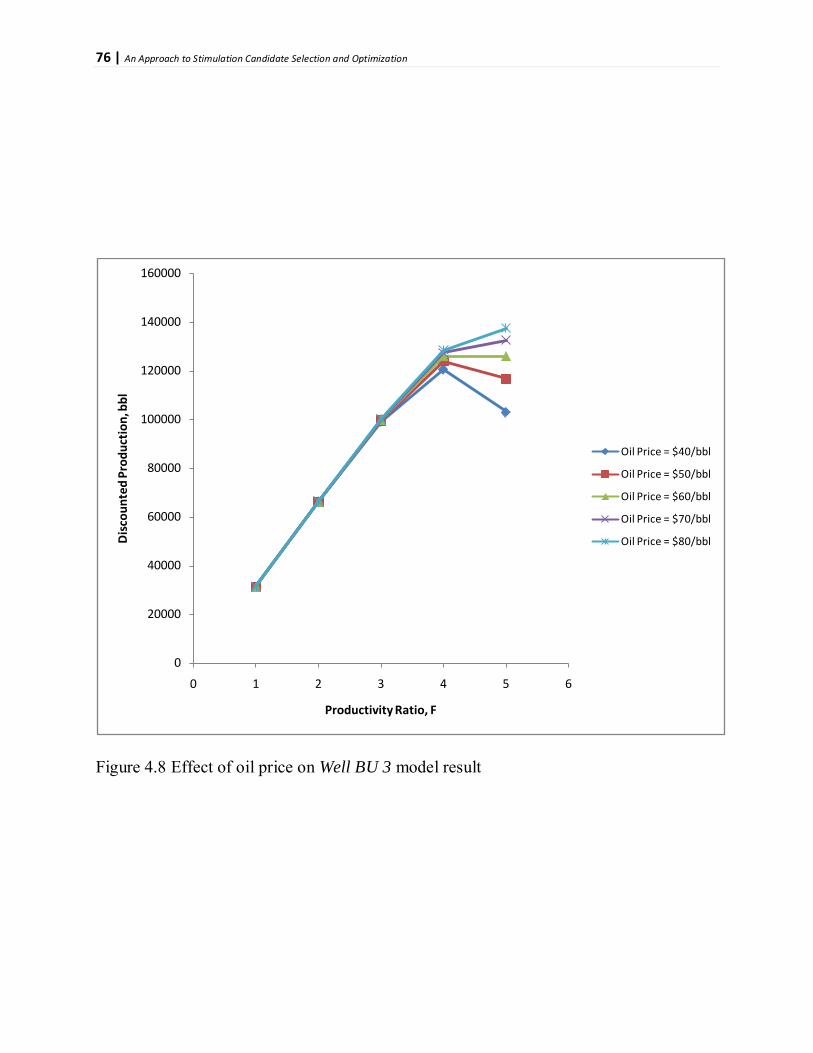
76 | An Approach to Stimulation Candidate Selection and Optimization
Figure 4.8 Effect of oil price on Well BU 3 model result
0
20000
40000
60000
80000
100000
120000
140000
160000
0 1 2 3 4 5 6
Dis
coun
ted
Prod
uctio
n, b
bl
Productivity Ratio, F
Oil Price = $40/bbl
Oil Price = $50/bbl
Oil Price = $60/bbl
Oil Price = $70/bbl
Oil Price = $80/bbl

77 | An Approach to Stimulation Candidate Selection and Optimization
4.3 Model Validation: Case Study 2
The data used for this case study was taken from published literatures by Nnanna et al.73, Nnanna
and A jienka76, a nd Onyekonwu80
4.3.1 Formulation of the Well BU 5 Model
. T hese data are used to formulate t he Well BU 5 Model. The
data for Well BU 5 is presented in Table 4.4.
Let’s assume that the remaining recoverable reserve in the drainage area of this well is 2.5 MM
bbls, and the tubing maximum design flow rate is 10000 stb/d. Also let’s assume that the price of
oil is $80/bbl, the effective discount rate is 10% and the maximum budget for the acidizing job is
set at $1000000.
The model is formulated as follows:
Step A:
The Cost versus Productivity-Ratio plot for Well BU 5 is shown in Fig. 4.9.
Enter t he da ta gi ven i nto t he A cidizing Design and Optimization Model and ge nerate
the Cost versus Productivity-Ratio data .
Step B:
For the input data, this equation is obtained as:
Obtain t he relationship be tween the s timulation c ost (C) a nd productivity ratio (F) in
form of power equation of a trendline through a log-log regression of the data.
𝐶𝐶 = 27.82𝐹𝐹6.187 ............…….….……….………..………4.9
The above relationship, as presented in Equation 4.1 was obtained from a regression analysis of
the model generated cost data using Microsoft Excel.
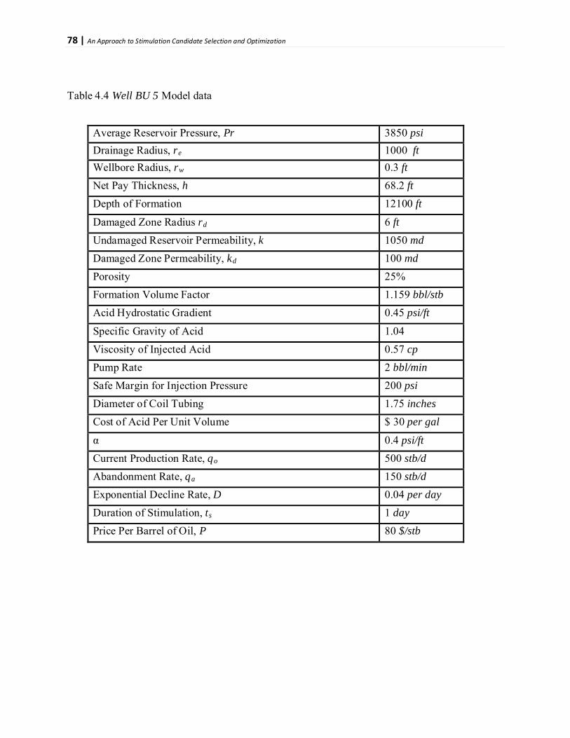
78 | An Approach to Stimulation Candidate Selection and Optimization
Table 4.4 Well BU 5 Model data
Average Reservoir Pressure, Pr 3850 psi Drainage Radius, r 1000 ft e Wellbore Radius, r 0.3 ft w Net Pay Thickness, h 68.2 ft Depth of Formation 12100 ft
Damaged Zone Radius r 6 ft d Undamaged Reservoir Permeability, k 1050 md Damaged Zone Permeability, k 100 md d Porosity 25% Formation Volume Factor 1.159 bbl/stb Acid Hydrostatic Gradient 0.45 psi/ft
Specific Gravity of Acid 1.04 Viscosity of Injected Acid 0.57 cp Pump Rate 2 bbl/min Safe Margin for Injection Pressure 200 psi Diameter of Coil Tubing 1.75 inches Cost of Acid Per Unit Volume $ 30 per gal
α 0.4 psi/ft Current Production Rate, q 500 stb/d o Abandonment Rate, q 150 stb/d a Exponential Decline Rate, D 0.04 per day Duration of Stimulation, t 1 day s Price Per Barrel of Oil, P 80 $/stb

79 | An Approach to Stimulation Candidate Selection and Optimization
Figure 4.9 Cost versus Productivity Ratio plot for Well BU 5.
0.00
200000.00
400000.00
600000.00
800000.00
1000000.00
1200000.00
1400000.00
1.00 1.50 2.00 2.50 3.00 3.50 4.00 4.50 5.00 5.50 6.00
Cost
, $
Productivity Ratio, F
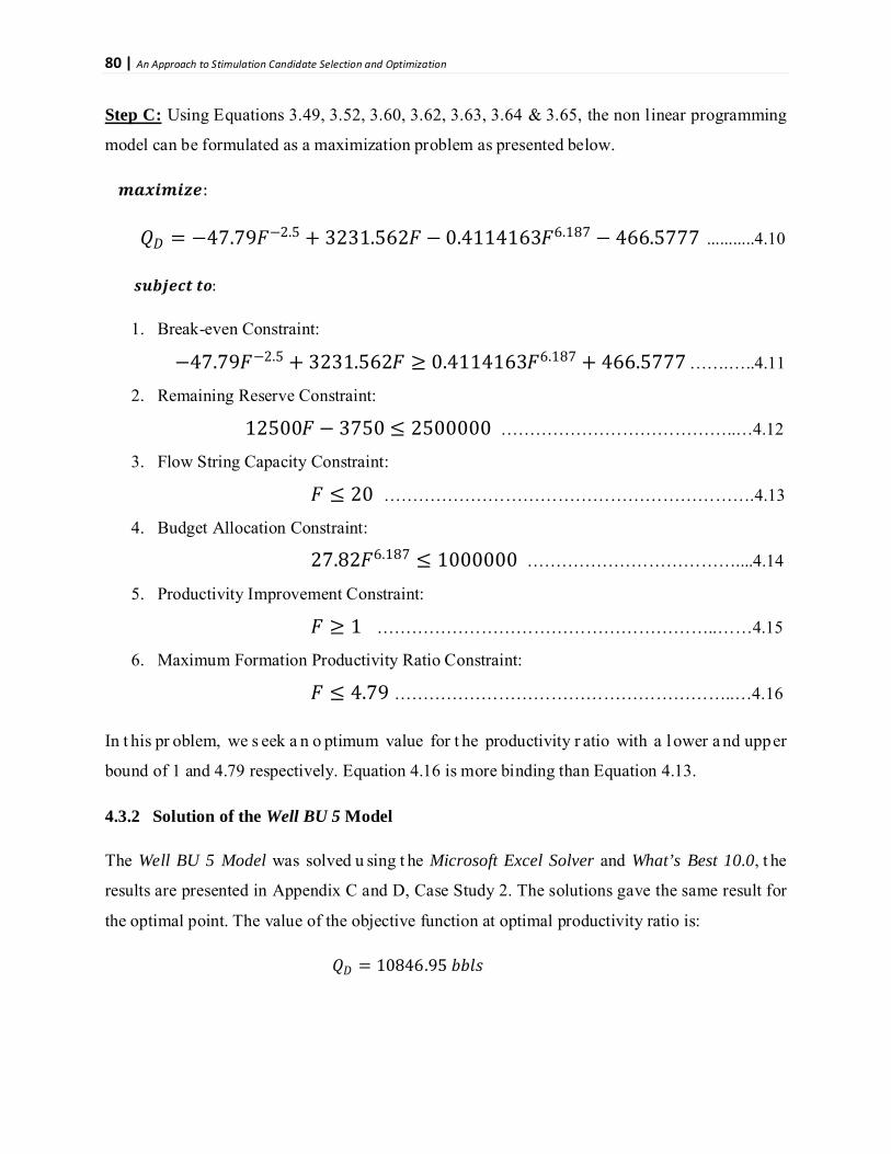
80 | An Approach to Stimulation Candidate Selection and Optimization
Step C:
𝒎𝒎𝒎𝒎𝒎𝒎𝒎𝒎𝒎𝒎𝒎𝒎𝒛𝒛𝒛𝒛:
Using Equations 3.49, 3.52, 3.60, 3.62, 3.63, 3.64 & 3.65, the non linear programming
model can be formulated as a maximization problem as presented below.
𝑄𝑄𝐷𝐷 = −47.79𝐹𝐹−2.5 + 3231.562𝐹𝐹 − 0.4114163𝐹𝐹6.187 − 466.5777 ...........4.10
𝒔𝒔𝒔𝒔𝒔𝒔𝒔𝒔𝒛𝒛𝒔𝒔𝒔𝒔 𝒔𝒔𝒕𝒕:
1. Break-even Constraint:
−47.79𝐹𝐹−2.5 + 3231.562𝐹𝐹 ≥ 0.4114163𝐹𝐹6.187 + 466.5777 …….…..4.11
2. Remaining Reserve Constraint:
12500𝐹𝐹 − 3750 ≤ 2500000 …………………………………..…4.12
3. Flow String Capacity Constraint:
𝐹𝐹 ≤ 20 ……………………………………………………….4.13
4. Budget Allocation Constraint:
27.82𝐹𝐹6.187 ≤ 1000000 ………………………………....4.14
5. Productivity Improvement Constraint:
𝐹𝐹 ≥ 1 …………………………………………………..……4.15
6. Maximum Formation Productivity Ratio Constraint:
𝐹𝐹 ≤ 4.79 …………………………………………………..…4.16
In t his pr oblem, we s eek a n o ptimum value for t he productivity r atio with a l ower a nd upper
bound of 1 and 4.79 respectively. Equation 4.16 is more binding than Equation 4.13.
4.3.2 Solution of the Well BU 5 Model
The Well BU 5 Model was solved u sing t he Microsoft Excel Solver and What’s Best 10.0, t he
results are presented in Appendix C and D, Case Study 2. The solutions gave the same result for
the optimal point. The value of the objective function at optimal productivity ratio is:
𝑄𝑄𝐷𝐷 = 10846.95 𝑏𝑏𝑏𝑏𝑏𝑏𝑏𝑏

81 | An Approach to Stimulation Candidate Selection and Optimization
The o ptimal p roductivity r atio i s e qual to 4 .18. The o bjective function be havior i s vi ewed
Mathematica 7.0. The plot generate i s shown i n Appendix E . Also, using Mathematica 7.0 to
solve t he n on-linear pr ogramming optimization pr oblem, the r esult for t he ob jective function i s
10276.7 bbls, while the value of the productivity ratio at the optimal point is 3.97. The solution
using Mathematica 7.0 is also shown in Appendix E.
The slight variation in the results obtained is due to same reasons as discussed in section 4.2.2.
4.3.3 Discussion of the Well BU 5 Model Result
This op timal v alue of t he o bjective f unction i s 10846.95 bbls, meaning th at i f th is well i s
considered f or s timulation, gi ven t hat the assumptions considered in s ection 4.3.1 a re binding,
the benefit derivable from the stimulation equals ($80/bbl × 10846.95 bbls ), i.e. $867,756.
The Answer Report for Case Study 2 –Section 1, in Solvers Result section of Appendix C shows
that t he six c onstraints a re n ot bi nding. T his m eans t hat t he o ptimal solution was f ound within
the limits of all the constraints. Hence no constraint is violated.
If we a ssume t hat t he stimulation budget a pproved by management i s $185,000 for t his well,
then t he ou tput o f t his model will be a s shown in Appendix C , Case Study 2 - Section 2 . T he
Answer Report Section shown that the budget allocation constraint is now binding. This means
that if management is willing to allocate more money to this project, there will be more benefit.
From the sensitivity report it could be seen that the value of the Lagrange Multiplier associated
with the budget allocation constraint is 0.0004047. Hence i f the stimulation budget is increased
by $1, the benefit derived from stimulation will increase by 0.0405%. This can be interpreted in
a much better sense a s $1 increase i n stimulation budget will r esult i n an additional production
benefit of 0.0004047 bbls.
The amount in dollars, X, needed to be added to the present budget in order to get an optimum
result can be roughly approximated with the following relationship (valid only for this case):
𝑋𝑋 ≈ 100𝜆𝜆∗𝑀𝑀1−100𝜆𝜆
………………………………………….….…4.17
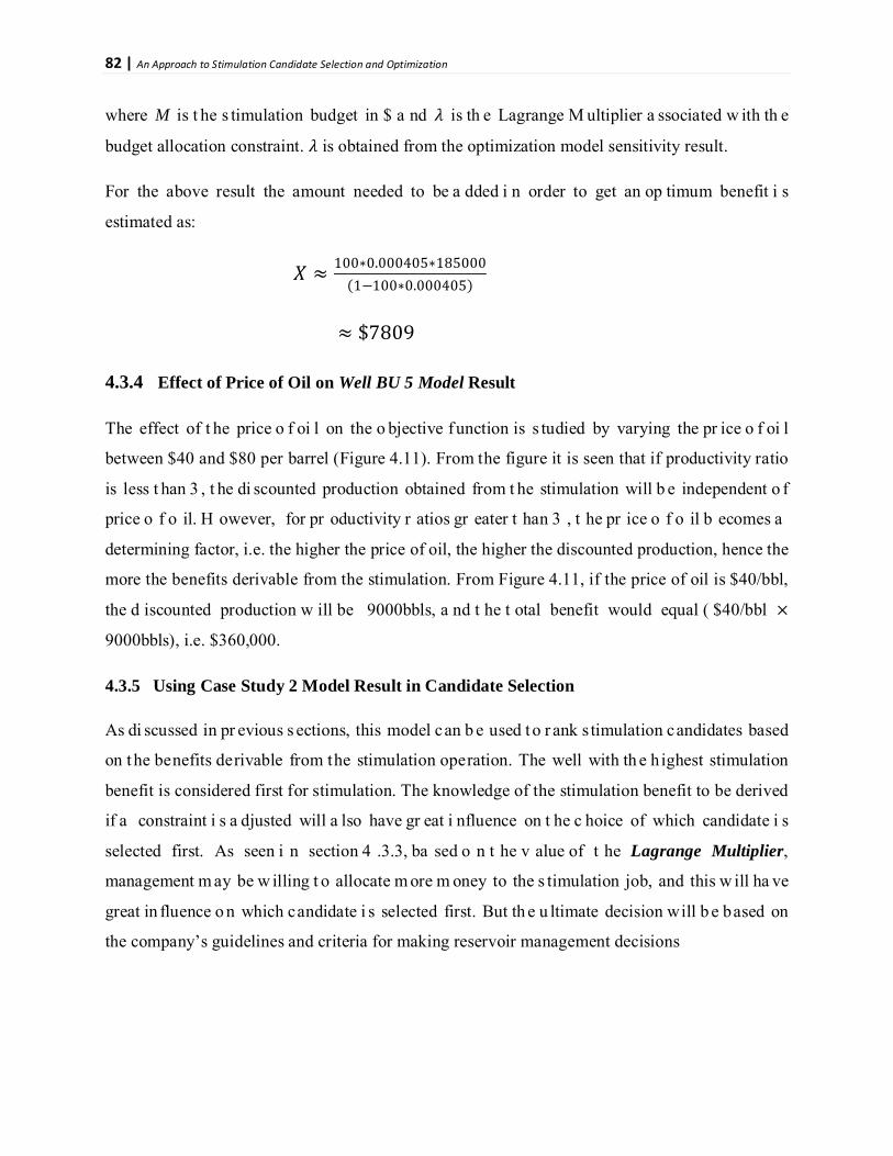
82 | An Approach to Stimulation Candidate Selection and Optimization
where M is t he s timulation budget in $ a nd 𝜆𝜆 is th e Lagrange M ultiplier a ssociated w ith th e
budget allocation constraint. 𝜆𝜆 is obtained from the optimization model sensitivity result.
For the above result the amount needed to be a dded i n order to get an op timum benefit i s
estimated as:
𝑋𝑋 ≈ 100∗0.000405∗185000(1−100∗0.000405)
≈ $7809
4.3.4 Effect of Price of Oil on Well BU 5 Model Result
The effect of t he price o f oi l on the o bjective function is s tudied by varying the pr ice o f oi l
between $40 and $80 per barrel (Figure 4.11). From the figure it is seen that if productivity ratio
is less t han 3 , t he di scounted production obtained from t he stimulation will b e independent o f
price o f o il. H owever, for pr oductivity r atios gr eater t han 3 , t he pr ice o f o il b ecomes a
determining factor, i.e. the higher the price of oil, the higher the discounted production, hence the
more the benefits derivable from the stimulation. From Figure 4.11, if the price of oil is $40/bbl,
the d iscounted production w ill be 9000bbls, a nd t he t otal benefit would equal ( $40/bbl ×
9000bbls), i.e. $360,000.
4.3.5 Using Case Study 2 Model Result in Candidate Selection
As di scussed in pr evious s ections, this model can b e used t o r ank s timulation candidates based
on t he benefits derivable from the stimulation operation. The well with th e highest stimulation
benefit is considered first for stimulation. The knowledge of the stimulation benefit to be derived
if a constraint i s a djusted will a lso have gr eat i nfluence on t he c hoice of which candidate i s
selected first. As seen i n section 4 .3.3, ba sed o n t he v alue of t he Lagrange Multiplier,
management m ay be w illing t o allocate m ore m oney to the s timulation job, and this w ill ha ve
great in fluence o n which candidate i s selected first. But th e u ltimate decision will b e based on
the company’s guidelines and criteria for making reservoir management decisions

83 | An Approach to Stimulation Candidate Selection and Optimization
Figure 4.10 Effect of oil price on Well BU 5 model result
0
2000
4000
6000
8000
10000
12000
0 1 2 3 4 5 6
Dis
coun
ted
Prod
uctio
n, b
bl
Productivity Ratio, F
Oil Price = $40/bbl
Oil Price = $50/bbl
Oil Price = $60/bbl
Oil Price = $70/bbl
Oil Price = $80/bbl

84 |An Approach to Stimulation Candidate Selection and Optimization
Chapter Five
Conclusion and Recommendations
5.1 Conclusion
This research seeks a method to quantify stimulation benefits derivable from different candidate
wells, a nd use the result t o rank economically profitable candidates. To achieve t his, a d esign
module was developed for a cidizing based o n t he works o f Schechter a nd G idley32, a nd
Economides and Nolte86
The o ptimization model derived i n t his r esearch c ombines the o utput from t he stimulation
treatment de sign m odule w ith production de cline c urve analysis and economic c ontinuous
discounting c oncepts. The o bjective f unction is f ormulated in the f orm of a no n-linear
programming pr oblem with some c onstraints. Hence, a constrained optimization p roblem is
presented. The s olution o f the objective function seeks a maximum di scounted production t hat
satisfies the constraints. The c onstraints considered i nclude those imposed b y the r emaining
recoverable oil i n p lace, t ubing string c apacity, maximum formation productivity a nd t he
stimulation budget approved by management.
. O ther design m odules were a lso developed f or gravel packing a nd
recompletion stimulation techniques.
To solve the objective function, a non-linear programming solver in Microsoft Excel and LINDO
Systems’ What is Best 10 were used to get an optimum solution. In all similar cases considered,
the s ame o ptimum s olutions were ob tained us ing either of t he t wo s olvers. Wolfram’s
Mathematica 7.0 was used to verify the solver’s results. They were found to be within acceptable
significant figures. Hence the results are correct and meaningful.
Field data ob tained f rom Bestfield offshore N iger D elta were u sed t o validate t he model. F our
candidate wells were selected for acidizing based on a well test data. The four wells are: Well BU
1, Well BU 2, Well BU 3 and Well BU 4. The application of the model to quantify the stimulation
benefits for each of t he four wells r eveals t hat t he Well BU 3 will h ave the g reatest e conomic
returns. Hence, Well BU 3 was ranked first for the stimulation treatment. In all cases, when using

85 |An Approach to Stimulation Candidate Selection and Optimization
this model, stimulation decisions should be based on the cost of the project, payout time and the
stimulation benefit.
A sensitivity a nalysis on t he r esults of t he m odel was a lso performed. B ased on t he s ensitivity
analysis and the results of the Bestfield Model, it can be concluded that:
1. The proposed methodology and models can be quantitatively used to estimate the benefits
derivable from stimulation options like: acidizing, gravel-packing and recompletion.
2. The mo del and non -linear o ptimization model can be u sed t o r ank c andidate w ells for
selective stimulation. Hence it can be used for stimulation candidate well selection.
3. Below a p roductivity r atio of 3, t he di scounted pr oduction from a cidizing does n ot
depend on the price of oi l. H owever, the ove rall m onetary be nefit derived fro m
stimulation depends on price of oil.
4. The optimization model can a lso be used to study t he effect o f t he t reatment parameters
on the objective function.
5.2 Recommendation
The following recommendations are presented to highlight areas of additional research to
improve the methodology and models developed in this research.
It is recommended that the model be used t o quantify stimulation be nefit derivable from a
stimulation decision o nce a well has been matched t o either of acidizing, gravel packing or
recompletion. F or e ffective use o f the model, i t i s r ecommended t hat t he l ease o perating cost
(LOE) and also, federal and state taxes be considered before ranking the wells for stimulation.
The effect of t he pr e-stimulation production rate on t he optimal point of t he objective function
(Fig. 4 .4) needs further investigations. S uch study will help to k now optimal t ime to initiate
stimulation jobs during the producing life of a well.
It i s al so r ecommended, for f urther s tudy, that a nother a pproach, other t hat t he pr oduction
decline curve analysis, that can be used to quantify the stimulation benefit be investigated. This

86 |An Approach to Stimulation Candidate Selection and Optimization
approach m ay combine inflow performance r elationship and other pressure da ta to obtain a
model that can be used to optimize the stimulation process.
It is further recommended that stimulation optimization correlations be developed, based on the
results of this model, that has a wide range of applications in the Niger Delta and other oil and
gas producing basins.

87 | An Approach to Stimulation Candidate Selection and Optimization
References
1. Civan, F .: Reservoir Formation Damage – Fundamentals, Modeling, Assesment and Mitigation, Gulf Publishing Company, Houston, Texas (2000) p.1
2. Bennion, B ., “Formation D amage—The I mpairment o f th e I nvisible, b y the
Inevitable and Uncontrollable, R esulting i n an Indeterminate Reduction of t he Unquantifiable!” Journal of Canadian Petroleum Technology, V ol. 3 8, No. 2, February 1999, pp. 11-17.
3. Porter, K. E ., “ An O verview of F ormation D amage,” Journal of Petroleum
Technology, Vol. 41, No. 8, 1989, pp. 780-786.
4. Mungan, N ., “Discussion o f an Overview o f F ormation D amage,” Journal of Petroleum Technology, Vol. 41, No. 11, Nov. 1989, p. 1224
5. Amaefule, J. O., Ajufo, A., Peterson, E., & Durst, K., "Understanding Formation
Damage Processes: An E ssential I ngredient for I mproved Measurement a nd Interpretation o f R elative P ermeability Data
," SPE 16232 paper, SPE Production Operations Symposium, 1987, Oklahoma City, Oklahoma
6. Van Everdingen, A.F. a nd H urst, W .: “The Application o f the L aplace
Transformation to Flow Problems in Reservoirs,” Trans., AIME (1949) 186, 305–324.
7. Hawkins, M.F.: “A Note on the Skin Effect,” Journal of Petroleum Technology (December 1956) 8, 356–357.
8. Frick, T .P. a nd Economides, M .J.: “ Horizontal We ll Damage Characterization and Removal,” SPE Production & Facilities (February 1993) 8, No. 1, pp.15–22.
9. Piot, B . M., & L ietard, O . M ., “Nature of Formation Damage in Reservoir
Stimulation,” in Economides, M. J . & Nolte, K. S., (eds.), Reservoir Stimulation, Schlumberger Education Services, Houston, Texas, 1987.
10. Economides, M.J., and Nolte, K.G., Reservoir Simulation, Third Edition. Wiley, N.Y. (hardbound) 2000, Chapter One, p. 1-12
11. Cinco-Ley, H., Ramey, H.J. Jr. and Miller, F.G.: “Pseudoskin Factors for Partially Penetrating D irectionally Drilled Wells,” paper SPE 5589, presented a t t he SPE Annual Technical C onference and Exhibition, Dallas, Texas, USA (September 28–October 1, 1975a).
88 | An Approach to Stimulation Candidate Selection and Optimization
12. Harris, M.H.: “The Effect of Perforating on Well Productivity,” paper SPE 1236, Journal of Petroleum Technology (April 1966) 18, pp. 518–528.
13. Karakas, M. a nd Tariq, S .: “Semi-Analytical Productivity Models for Perforated Completions,” paper S PE 18247, p resented a t t he S PE Annual Technical Conference and Exhibition, Houston, Texas, USA (October 2–5, 1988).
14. Economides, M.J., and N olte, K.G., Reservoir Simulation, Third Edition. W iley, N.Y. (hardbound) 2000, Chapter One, p. 1-13
15. Yan, J ., J iang, G ., & Wu, X., “Evaluating o f F ormation D amage C aused by Drilling a nd Completion Fluids i n H orizontal W ells,” Journal of Canadian Petroleum Technology, Vol. 36, No. 5, 1997, pp. 36-42.
16. McLeod, Jr., H. O and Coulter, Jr., A. W.: “The Stimulation Treatment Pressure Record – An Overlooked Formation Evaluation Tool” Journal of Petroleum Technology (August, 1969) p. 952
17. Raymond, L . R . a nd H udson, J . L .: “ Short-Term Well Te sting to D etermine Wellbore Damage”, Journal of Petroleum Technology (Oct. 1966) 1363-1370
18. Amaefule, J. O., Kersey, D. G., Norman, D. L., & Shannon, P. M., “Advances in Formation Da mage Assessment a nd C ontrol Strategies,” CIM Paper No. 88 -39-65, Proceedings of t he 39th Annual Technical Meeting o f P etroleum S ociety of CIM an d C anadian G as P rocessors Association, Ju ne 1 2-16, 1988, C algary, Alberta, 16 p. 65-2
19. Muskat, M., The Flow of Homogeneous Fluids Through Porous Media, McGraw-Hill Book Co., New York, New York, 1937
20. Civan, F .: Reservoir Formation Damage – Fundamentals, Modeling, Assesment and Mitigation, Gulf Publishing Company, Houston, Texas (2000) p.688
21. Leontaritis, K. J ., “Asphaltene Ne ar-Wellbore F ormation D amage Modeling,” SPE 39446 p aper, P roceedings of t he 1998 S PE Formation Damage C ontrol Conference, February 18-19, 1998, Lafayette, Louisiana, pp. 277-288.
22. Civan, F .: Reservoir Formation Damage – Fundamentals, Modeling, Assesment and Mitigation, Gulf Publishing Company, Houston, Texas (2000) p.688
23. Zhu, D ., H ill, A. D ., & Morgenthaler, L . N ., “ Assessment o f M atrix Ac idizing Treatment R esponses i n G ulf of M exico W ells,” Proceedings of t he 199 9 S PE Mid-Continent Operations Symposium held in Oklahoma City, Oklahoma, USA, March 28-31, 1999.
89 | An Approach to Stimulation Candidate Selection and Optimization
24. Mukherjee, H ., & Economides, M. J ., “A Parametric Co mparison of Horizontal
and Vertical Well Performance,” SPE Formation Evaluation, June 1991, pp. 209-216.
25. Civan, F .: Reservoir Formation Damage – Fundamentals, Modeling, Assesment and Mitigation, Gulf Publishing Company, Houston, Texas (2000) p.687
26. Li, Y -H., Fambrough, J . D ., & Montgomery, C. T ., “ Mathematical M odeling of Secondary P recipitation f rom Sandstone A cidizing,” SPE Journal, December 1998, pp. 393-401
27. Lee, J ., & Kasap, E ., “Fluid Sampling from D amaged Formations,” SPE 39817 paper, P roceedings of t he 1998 S PE P ermian B asin O il a nd G as Recovery Conference, March 25-27, 1998, Midland, Texas, pp. 565-570.
28. Economides, M.J., Hill, A.D. and Ehlig-Economides, C.A.: Petroleum Production Systems, Englewood Cliffs, New Jersey, USA, Prentice-Hall (1994) p.350
29. Williams, B . B ., G idley, J . L . a nd S chechter, R . S .: Acidizing Fundamentals, Monograph Series vol. 6, SPE, Dallas, TX, (1979), p. 68
30. Dullien, F. A. L.: “Pore Structure Analysis,” paper presented at the ACS State-of-the-Art Summer S ymposium, Div. Ind. Eng. C hem., Washington, D. C. (June, 1969).
31. Scheidegger, A. E: The Physics of Flow Through Porous Media, The Macmillian Co., New York (1960).
32. Schechter, R. S. and Gidley, J . L.: “The Change i n Pore Size Distribution From Surface Reactions in Porous media,” AIChE Journal (May 1969) 15, pp. 339-350
33. Walsh, M. P ., L ake, L . W ., a nd S chechter, R . S .: “ A D escription o f C hemical Precipitation Mechanism and Their Role in Formation Damage during Stimulation b y H ydrofluoric Acid,” Journal of Petroleum Technology, (September 1982) pp. 2097-2112.
34. Sevougian, S . D ., L ake, L . W ., a nd S chechter, R . S .: “ A N ew G eochemical Simulator to Design More Effective Sandstone Acidizing Treatment,” SPE paper 24780, 1992.
35. Quinn, M . A., Lake, L arry W . a nd S chechter, R obert S.: "Designing E ffective Sandstone A cidizing Treatments Through Geochemical Modeling," S PE 38173 presented at the 1997 European Formation Damage Conference, The Hague, June 2-3, 1997.

90 | An Approach to Stimulation Candidate Selection and Optimization
36. Taha, R ., H ill, A. D ., a nd S epehmoori, K., “ Sandstone Acidizing D esign with a Generalized Model,” SPE Production Engineering, (Feb. 1989), pp. 49-55.
37. Hekim, Y ., Fogler, H . S., a nd M cCune, C . C .: “ The Radial M ovement of Permeability F ronts a nd M ultiple R eaction Z ones i n P orous Media,” Journal of Petroleum Technology, pp. 99-107, February 1982
38. da Motta, E . P ., P lavnik, B., and Schechter, R . S .: “Optimizing Sandstone acidizing,” SPE Reservoir Engineering, (February 1992a), pp. 149-153,.
39. Sumotarto, U ., Hill, A . D ., and S epehrnoori, K .: “An Integrated S andstone Acidizing Fluid Selection a nd Simulation to Optimize Treatment D esign,” SPE paper 30520 presented at t he SPE Annual T echnical C onference & Exhibition held in Dallas, TX, U.S.A., (Oct., 1995) pp. 22-25.
40. Gdanski, R. D ., a nd S huchart, C . E.: “ Advanced Sandstone Acidizing D esigns With Improved R adial M odels,” S PE paper 52397 p resented at the 199 7 SPE Annual T echnical Conference a nd E xhibition h eld i n S an A ntonio, T exas,(Oct. 1998), pp. 5-8.
41. Hill, A. D., Lindsay, D . M., Silberberg, I . H., and Schechter, R. S.: “Theoretical
and E xperimental S tudies of Sandstone A cidizing,” Journal of Petroleum Technology, (Feb. 1981), pp. 30-42.
42. Hekim, Y ., Fogler, H . S., a nd McCune, C . C., “ The R adial Movement of Permeability Fronts a nd Multiple R eaction Zones i n Porous M edia,” Journal, (Feb. 1982), pp. 99-107.
43. Schechter, R. S., Oil Well Stimulation, Prentice Hall, Englewood Cliffs, NJ, 1992.
44. Economides, M.J., and N olte, K.G., Reservoir Simulation, Third Edition. W iley, N.Y. (hardbound) 2000, Chapter 13, p. 16-13.
45. Bryant, S.L.: “An I mproved Model of Mud A cid/Sandstone Chemistry,” paper SPE 22855, presented a t the SPE Annual Technical C onference and Exhibition, Dallas, Texas, USA (October 6–9, 1991).
46. da M otta, E.P., Plavnik, B ., S chechter, R .S. a nd H ill, A.D.: “ The Relationship Between Reservoir Mineralogy a nd O ptimum Sandstone Acid T reatment,” paper SPE 23802, presented at the SPE International Symposium on Formation Damage Control, Lafayette, Louisiana, USA (February 26–27, 1992b).
47. Sumotarto, U .: “Sandstone A cidizing S imulation: Development of an E xpert System,” PhD dissertation, T he University of T exas a t Austin, Au stin, T exas, USA (1995).
91 | An Approach to Stimulation Candidate Selection and Optimization
48. Economides, M.J., Hill, A.D. and Ehlig-Economides, C.A.: Petroleum Production
Systems, Englewood Cliffs, New Jersey, USA, Prentice-Hall (1994) p.359
49. Guin, J.A., Schechter, R.S. and Silberberg, I.H.: “Chemically Induced Changes in Porous Media,” Ind. & Eng. Chem. Fund. (February 1971) 10, No.1, pp. 50–54.
50. Labrid, J .C.: “Thermodynamic and Kinetic Aspects of Argillaceous S andstone Acidizing,” paper SPE 5165, Journal of Petroleum Technology (April 1975), pp. 117–128.
51. Lambert, M.E.: “A Statistical Study of Reservoir Heterogeneity,” MS thesis, The University of Texas at Austin, Austin, Texas, USA (1981).
52. Lund, K. a nd Fogler, H .S.: “ Acidization V. T he Prediction of t he M ovement o f Acid a nd P ermeability F ronts i n S andstone,” Chemical Engineering Science (1976) 31, No. 5, pp. 381–392.
53. McLeod, H .O. J r.: “Matrix Acidizing,” paper SPE 13752, Journal of Petroleum Technology (December 1984) 36, pp. 2055–2069.
54. Shaughnessy, C.M. and Kunze, K.R.: “Understanding Sandstone Acidizing Leads to Improved Field Practices,” paper SPE 9388, Journal of Petroleum Technology (July 1981), pp. 1196–1202.
55. Hoefner, M.L. and Fogler, H.S.: “Pore Evolution and Channel Formation During Flow and Reaction in Porous Media,” AIChEJ. (Jan., 1988) 34, No.1, pp. 45–54.
56. Hung, K.M., Hill, A.D. and Sepehrnoori, K.: “A Mechanistic Model of Wormhole Growth i n Carbonate Matrix A cidizing a nd Acid Fracturing,” paper SPE 16886, Journal of Petroleum Technology, (January 1989) 41, No. 1, 59–66.
57. Daccord, G ., T ouboul, E . a nd L enormand, R .: “ Carbonate A cidizing: T oward a Quantitative M odel of t he Wormholing Phenomenon,” p aper SPE 16887, SPE Production Engineering (February 1989), pp. 63–68.
58. Pichler, T., Frick, T.P., Economides, M.J. and Nittmann, J.: “Stochastic Modeling of W ormhole Growth i n C arbonate A cidizing with B iased R andomness,” pa per SPE 25004, p resented a t t he S PE European P etroleum C onference, Cannes, France (November 16–18, 1992).
59. Economides, M.J., Hill, A.D. and Ehlig-Economides, C.A.: Petroleum Production Systems, Englewood Cliffs, New Jersey, USA, Prentice-Hall (1994) p.400
60. Fredd, C.N. and Fogler, H.S.: “Influence of Transport and Reaction on Wormhole Formation in Porous Media,” AIChE J. (September 1998b), pp. 1933–1949.
92 | An Approach to Stimulation Candidate Selection and Optimization
61. Ben-Naceur, K., E conomides, M . J .: “ The E ffectiveness of Acid Fractures an d
Their Production Behaviour,” Spe Paper 18536, 1988.
62. Lo, K. K., a nd Dean, R . H.: “ Modeling of Acid Fracturing,” SPE Production Engineering, (May, 1989), pp. 194-200.
63. Settari, A.: “Modelling of Acid Fracturing Treatment,” paper SPE 21870, 1991.
64. Nierode, D .E. a nd Williams, B.B.: “ Characteristics of Acid R eactions in Limestone Formations,” paper SPE 3101, presented at the SPE Annual Meeting, Houston, Texas, USA (Oct. 4-7, 1971); also in Journal of Petroleum Technology (Dec., 1971), pp. 408-418.
65. Nierode, D.E. a nd Kruk, K.F.: “An Evaluation of A cid F luid Loss A dditives, Retarded Acids and Acidized Fracture Conductivity,” paper SPE 4549, presented at the SPE Annual Meeting, Las Vegas, Nevada, USA (Sept. 30–Oct. 3, 1973).
66. Bennett, C . O .: “ Analysis Fractured W ells,” P h. D. t hesis, University of Tulsa, Tulsa, Oklahoma, 1982.
67. Ben-Naceur, K., an d E conomides, M. J .: “ Acid Fracture Propagation an d Production” i n Reservoir Stimulation, M . J . E conomides a nd K. G . N olte, e ds., Prentice Hall, Englewood Cliffs, NJ, Chap. 18, 1989.
68. Prats, M.: “Effects of Vertical Fractures on Reservoir Behaviour – Incompressible Fluid Case,” paper SPE 1575-G, Journal of Petroleum Technology, (June 1961) 1, No. 1, pp. 105-118; also in Trans., AIME (1961) 222.
69. Agarwal, R . G., Carter, R. D., and Pollock, C. B.: “Evaluation a nd Prediction of Performance o f L ow-Permeability Gas We lls S timulated b y M assive Hydraulic Fracturing,” Journal of Petroleum Technology (March, 1979), Trans. AIME, 267, pp 362-372.
70. Cinco-Ley, H. and Samaniego-V., F.: “Transient Pressure Analysis for Fractured Wells,” paper S PE 7490, Journal of Petroleum Technology (September 1981b) 33, 1749–1766.
71. Cinco-Ley, H ., Samaniego-V., F . an d D ominguez, N .: “ Transient P ressure Behavior for a W ell with a F inite-Conductivity V ertical F racture,” paper SPE 6014, p resented a t the SPE Annual T echnical C onference a nd E xhibition, N ew Orleans, L ouisiana, USA ( October 3 –6, 1976) ; a lso i n Journal of Petroleum Technology (August 1978) 18, 253–264.

93 | An Approach to Stimulation Candidate Selection and Optimization
72. Rae, P., and Di Lullo, G.: “Achieving 100 Percent Success in Acid Stimulation of Sandstone R eservoirs,” paper SPE 77808, presented a t the SPE Asia Pacific Oil Conference and Exhibition held in Melbourne, Australia (Oct. 8-10, 2002).
73. Nnanna E., O suagwu M., a nd Okereke O.: “ Important C onsiderations i n Matrix Stimulation Candidate Selection in Niger Delta”, paper SPE 128604 presented at the 2009 SPE Annual International Conference and Exhibition, Abuja (Aug 3-5).
74. Nitters, G., Roodhart, L., Jongma, H., Yeager, V., Buijse, M., Fulton, D., Dahl, J., and J antz, E. : “ Structured Approach t o Advanced C andidate Selection a nd Treatment Design of Stimulation Treatments,” paper SPE 63179, presented at the 2000 SPE Annual Technical Conference a nd Exhibition held in D allas, T exas (Oct. 1-4).
75. Jones, L . G.: c ourse no tes, Formation Damage School, Mobil, Duncan, OK (March 1989).
76. Nnanna, E; Ajienka, J : “Critical Success Factors for W ell Stimulation”, p aper SPE 98823 p resented a t t he 2005 N igerian Annual C onference & E xhibition, Abuja (August 1-3).
77. Al Qahtani, A., and Al Shehri, D.: “The Ec-Factor: A Correlation for Optimizing Completion Efficiency,” paper SPE 81490 presented at the 2003 SPE Middle East Oil Show, Bahrain (April 5-8).
78. Yildiz, Y .: “ Assessment of T otal Skin Factor i n Perforated W ells,” p aper S PE 82249 presented a t t he 2003 SPE European Formation Damage Conference, The Hague (May 13-14).
79. Lee, W. J.: Well Testing, Society of Petroleum Engineers Textbook (1982).
80. Onyekonwu, M. O.: Principles of Bottomhole Pressure Testing, Laser Publishers Ltd, Port Harcourt. p 91.
81. Afolabi, A, O pusunju A , H enri J , O nyekwere C letus, O nyekwere C hris a nd Davalos J.: “Increasing Production in a Brown Field with Heavy Crude and Fines Problem by Application of a N ew H F-Acid System: Case Histories” paper SPE 112558 p resented a t the 2008 S PE I nternational S ymposium on Formation Control, Lafayette, Louisiana (Feb 13-15).
82. Jennings, A. R .: “ Good Wells Make th e B est Candidates for W ell Stimulation,” SPE Production Engineering (Nov., 1991), pp 371-376.
83. Kartoatmodjo, G ., C aretta, F ., F lew, S ., J adid, M .: “ Risk-Based C andidate Selection W orkflow I mprove Acid S timulation S uccess R atio i n M ature F ield,” paper SPE 109278 presented at the 2007 SPE Asia Pacific Oil & Gas Conference, Jarkata, Indonesia (Oct. 30 to Nov. 1st).
94 | An Approach to Stimulation Candidate Selection and Optimization
84. Al-Araimi, M ., M ahajan, M.: “Successful Revival o f L ong-term C losed-in Ga s
Well by Right Matrix Stimulation Treatment,” paper SPE 96735 presented at the 2005 SPE Annual Technical Conference & Exhibition, Dallas, TX (Oct. 9-12).
85. Sinson, C . M ., O gbe, D . O ., D ehghani, K., “ Optimization of W ell Stimulation Strategies in Oil and Gas Fields,” paper SPE 17792, 1988.
86. Economides, M.J., and N olte, K.G., Reservoir Simulation, Third Edition. W iley, N.Y. (hardbound) 2000, Chapter Eighteen, p. 24-25.
87. Strubhar, M. K., Blackburn, J. S., and Lee, J. W.: “Production Operations Course II: Well Diagnosis,” Lecture Notes for a Video-Tape Course, SPE, Dallas (1972), pp. 525-544.
88. Vogt, T. C., Anderson, M. L.: “Optimizing the Profitability of Matrix Acidizing Treatments,” pa per SPE 4550 (preprint) presented at the SPE AIME 48th
Annual Fall Meeting, Las Vegas, Nev., Sept. 30- Oct. 3, 1973. (Revised manuscript, May 13, 1974).
89. Ofoh, E . P ., and Heikal S.: “ Reservoir M anagement Optimization through a Systematic Removal of Formation D amage, a C ase Study of Okpoho F ield in Niger-Delta”, paper presented at the 30th Annual SPE I nternational Technical Conference and Exhibition in Abuja, Nigeria, July 31- August 2, 2006.

95 | An Approach to Stimulation Candidate Selection and Optimization
Nomenclature
𝐶𝐶𝑔𝑔𝑔𝑔 cost of gravel packing, $
𝐶𝐶𝑔𝑔 cost of gravel, $/ft
𝐶𝐶𝑐𝑐𝑐𝑐 cost of carrier fluid (base fluid), $/bbl
3
Cmax
𝑐𝑐𝑠𝑠𝑠𝑠 cost of acid used per unit volume, $/gal
Maximum Stimulation Budget, $
𝐶𝐶𝑔𝑔𝑝𝑝𝑝𝑝𝑐𝑐 cost of perforation, $
𝑑𝑑 diameter of pipe, inches
𝑑𝑑𝑔𝑔 diameter of perforation tunnel, inches
𝐷𝐷 decline rate, per day
𝐹𝐹𝑠𝑠𝑚𝑚𝑚𝑚 maximum productivity ratio, dimensionless
𝐹𝐹 stimulation productivity ratio, dimensionless
𝑔𝑔𝑐𝑐 fracture gradient, psi/ft
qmax
h thickness of the oil sand, ft
tubing maximum design flowrate, stb/day
ℎ𝑔𝑔 perforated interval length, ft
I effective discount rate per day, %
𝐼𝐼𝑚𝑚𝑎𝑎𝑎𝑎 index of anisotropy
𝐼𝐼𝐷𝐷𝑐𝑐𝑠𝑠𝑔𝑔 inner diameter of the casing string, inches
𝐾𝐾𝐻𝐻 horizontal permeability, md
𝐾𝐾𝑉𝑉 vertical permeability, md
𝑘𝑘𝑝𝑝 reservoir permeability, md
𝑘𝑘𝑑𝑑𝑔𝑔 permeability of compacted zone around perforation in rock, md

96 | An Approach to Stimulation Candidate Selection and Optimization
𝑘𝑘𝑔𝑔𝑔𝑔 permeability of the gravel-pack gravel, md
𝑘𝑘 reservoir permeability, md
𝐿𝐿𝑔𝑔 length of flow path through gravel pack, inches
𝐿𝐿𝑠𝑠𝑐𝑐𝑝𝑝𝑝𝑝𝑝𝑝𝑎𝑎 length of the screen, ft
𝐿𝐿𝑏𝑏𝑏𝑏𝑚𝑚𝑎𝑎𝑘𝑘 length of the blank string, ft
𝐿𝐿𝑔𝑔 depth of penetration in rock, ft
𝑎𝑎 number of perforations
𝑎𝑎𝑔𝑔𝑝𝑝𝑝𝑝𝑐𝑐 number of perforations open
𝑂𝑂𝐷𝐷𝑏𝑏𝑏𝑏𝑚𝑚𝑎𝑎𝑘𝑘 outer diameter of the blank string, inches
𝑂𝑂𝐷𝐷𝑠𝑠𝑐𝑐𝑝𝑝𝑝𝑝𝑝𝑝𝑎𝑎 outer diameter of the screen, inches
𝑃𝑃𝑠𝑠 ,𝑠𝑠𝑚𝑚𝑚𝑚 maximum surface pressure, psi
Pr average reservoir pressure, psi
P price per barrel of oil, $
𝑞𝑞𝑑𝑑 damaged flow rate, stb/day
𝑞𝑞 damaged standard flow rates, stb/day
𝑞𝑞𝑎𝑎 initial production rate, stb/day
𝑞𝑞𝑜𝑜 the production rate, stb/day
𝑝𝑝𝑝𝑝 reservoir drainage radius, ft
𝑝𝑝𝑑𝑑 damaged zone radius, ft
𝑝𝑝𝑤𝑤 wellbore radius, ft
𝑝𝑝𝑑𝑑𝑔𝑔 radius of compacted zone around the perforations, ft
𝑝𝑝𝑔𝑔 radius of perforation in rock, ft
ROIP remaining recoverable reserve, bbl
𝑠𝑠𝑐𝑐+𝜃𝜃 skin effect caused by partial completion and slant, dimensionless
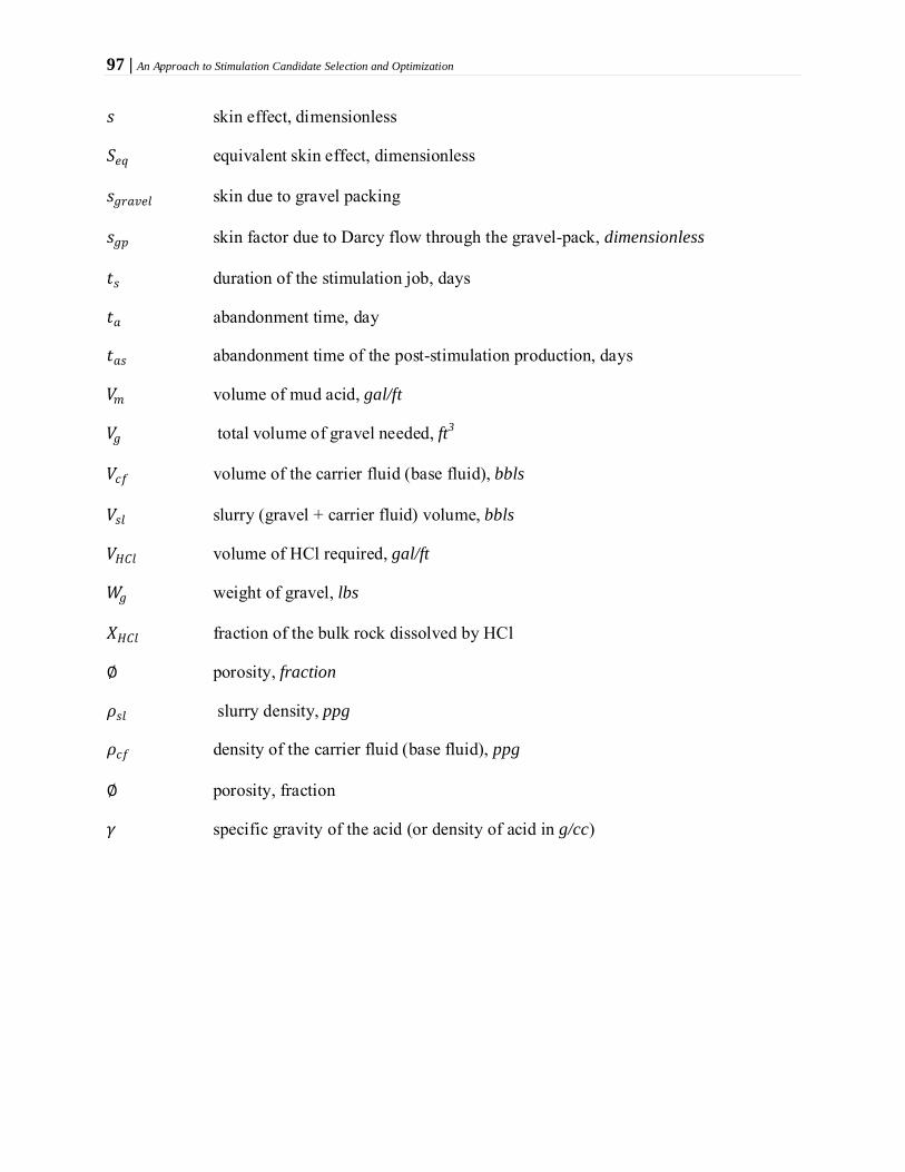
97 | An Approach to Stimulation Candidate Selection and Optimization
𝑠𝑠 skin effect, dimensionless
𝑆𝑆𝑝𝑝𝑞𝑞 equivalent skin effect, dimensionless
𝑠𝑠𝑔𝑔𝑝𝑝𝑚𝑚𝑔𝑔𝑝𝑝𝑏𝑏 skin due to gravel packing
𝑠𝑠𝑔𝑔𝑔𝑔 skin factor due to Darcy flow through the gravel-pack, dimensionless
𝑡𝑡𝑠𝑠 duration of the stimulation job, days
𝑡𝑡𝑚𝑚 abandonment time, day
𝑡𝑡𝑚𝑚𝑠𝑠 abandonment time of the post-stimulation production, days
𝑉𝑉𝑠𝑠 volume of mud acid, gal/ft
𝑉𝑉𝑔𝑔 total volume of gravel needed, ft
𝑉𝑉𝑐𝑐𝑐𝑐 volume of the carrier fluid (base fluid), bbls
3
𝑉𝑉𝑠𝑠𝑏𝑏 slurry (gravel + carrier fluid) volume, bbls
𝑉𝑉𝐻𝐻𝐶𝐶𝑏𝑏 volume of HCl required, gal/ft
𝑊𝑊𝑔𝑔 weight of gravel, lbs
𝑋𝑋𝐻𝐻𝐶𝐶𝑏𝑏 fraction of the bulk rock dissolved by HCl
∅ porosity, fraction
𝜌𝜌𝑠𝑠𝑏𝑏 slurry density, ppg
𝜌𝜌𝑐𝑐𝑐𝑐 density of the carrier fluid (base fluid), ppg
∅ porosity, fraction
𝛾𝛾 specific gravity of the acid (or density of acid in g/cc)
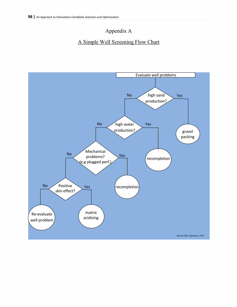
98 | An Approach to Stimulation Candidate Selection and Optimization
Appendix A
A Simple Well Screening Flow Chart
Positive skin effect?
No
No Yes
gravel packing
Mechanical problems?
(e.g plugged perf.)
matrix acidizing
high sand production?
No Yes
high water production?
No Yes
Yes recompletion
recompletion
Benson Best Ugbenyen, 2010
Evaluate well problems
Re-evaluate well problem
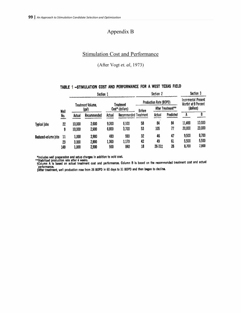
99 | An Approach to Stimulation Candidate Selection and Optimization
Appendix B
(After Vogt et. al, 1973)
Stimulation Cost and Performance

100 | An Approach to Stimulation Candidate Selection and Optimization
Appendix C
Solver Results
CASE STUDY 1
Well BU 1 Model output result

101 | An Approach to Stimulation Candidate Selection and Optimization
Solver Answer Report for Well BU 1 Model

102 | An Approach to Stimulation Candidate Selection and Optimization
Solver Sensitivity Report for Well BU 1 Model

103 | An Approach to Stimulation Candidate Selection and Optimization
Solver Limits Report for Well BU 1 Model

104 | An Approach to Stimulation Candidate Selection and Optimization
Well BU 2 Model output result

105 | An Approach to Stimulation Candidate Selection and Optimization
Well BU 3 Model output result

106 | An Approach to Stimulation Candidate Selection and Optimization
Solver Answer Report for Well BU 3 Model

107 | An Approach to Stimulation Candidate Selection and Optimization
Solver Sensitivity Report for Well BU 3 Model

108 | An Approach to Stimulation Candidate Selection and Optimization
Solver Limits Report for Well BU3 Model

109 | An Approach to Stimulation Candidate Selection and Optimization
Well BU 4 Model output result

110 | An Approach to Stimulation Candidate Selection and Optimization
CASE STUDY 2
– Section 1
Solver answer report for Well BU 5 model
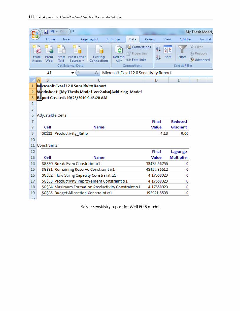
111 | An Approach to Stimulation Candidate Selection and Optimization
Solver sensitivity report for Well BU 5 model

112 | An Approach to Stimulation Candidate Selection and Optimization
Solver limit report for Well BU 5 model
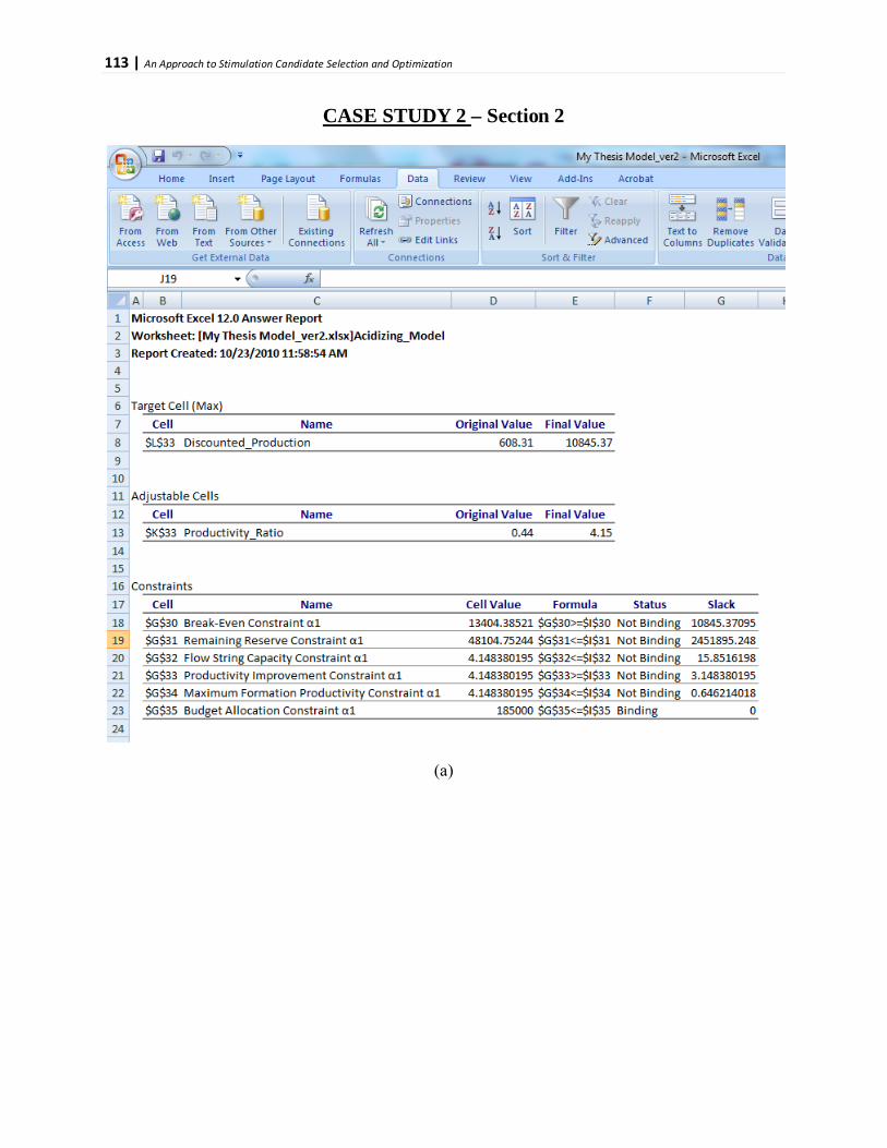
113 | An Approach to Stimulation Candidate Selection and Optimization
CASE STUDY 2
– Section 2
(a)
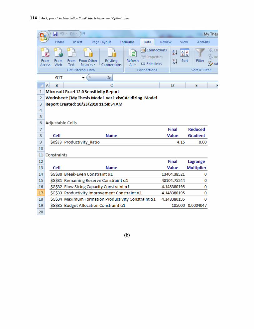
114 | An Approach to Stimulation Candidate Selection and Optimization
(b)
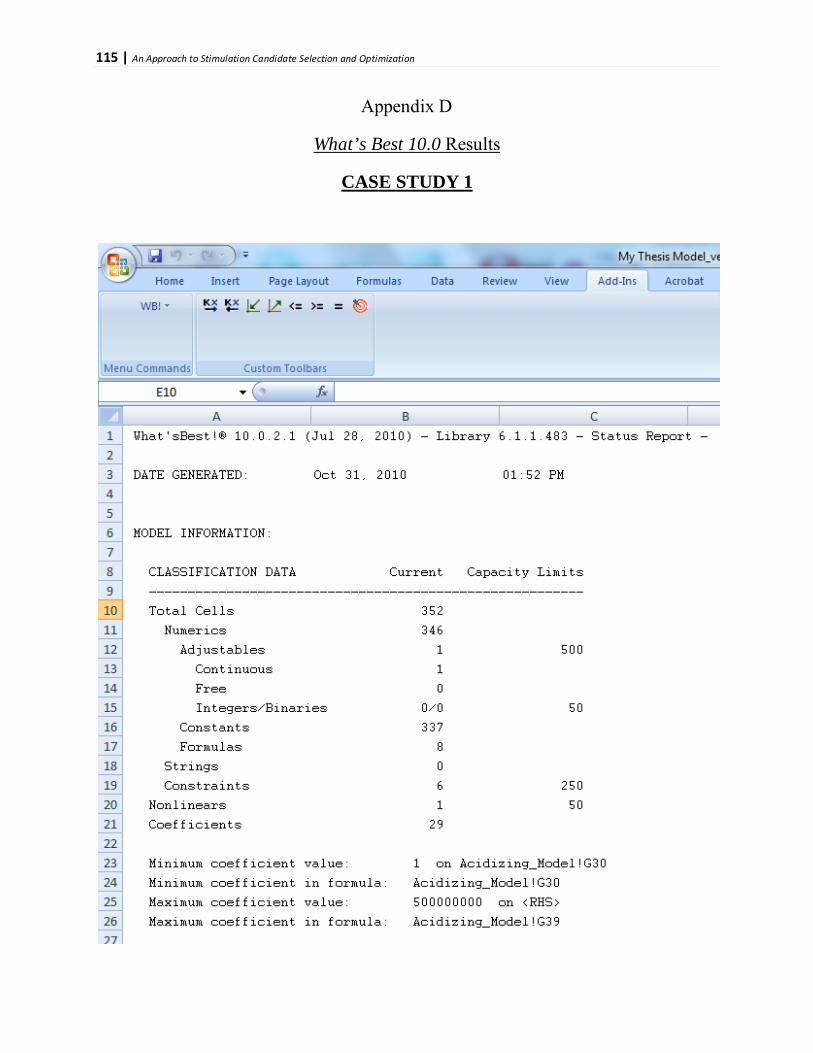
115 | An Approach to Stimulation Candidate Selection and Optimization
Appendix D
What’s Best 10.0 Results
CASE STUDY 1
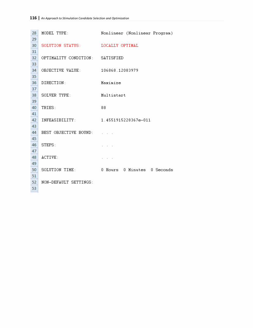
116 | An Approach to Stimulation Candidate Selection and Optimization
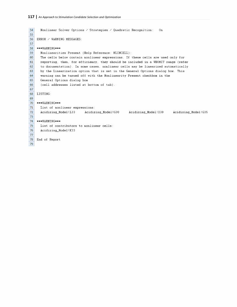
117 | An Approach to Stimulation Candidate Selection and Optimization

118 | An Approach to Stimulation Candidate Selection and Optimization
CASE STUDY 2

119 | An Approach to Stimulation Candidate Selection and Optimization

120 | An Approach to Stimulation Candidate Selection and Optimization
Appendix E
Mathematica 7.0 Results
CASE STUDY 1
Mathematica 7.0 plot of the objective function for Well BU 3 Model

121 | An Approach to Stimulation Candidate Selection and Optimization
Mathematica 7.0 input syntax and results for Well BU 3 Model

122 | An Approach to Stimulation Candidate Selection and Optimization
Mathematica 7.0 inpretation of input data and results for Well BU 3 Model
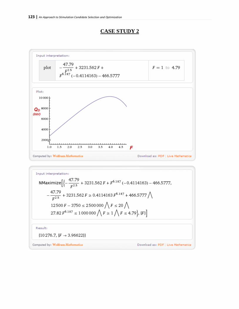
123 | An Approach to Stimulation Candidate Selection and Optimization
CASE STUDY 2

124 | An Approach to Stimulation Candidate Selection and Optimization
Appendix F
The derivation of the optimization model presented in this section is modified from the published work of Sinson et al.
Derivation of the Objective Function for Other Decline Cases
85
F.1
Let u s start by deriving t he o ptimization model for the general decline curve analysis.
The general decline curve equation is given by:
General Decline Curve Optimization
𝑞𝑞(𝑡𝑡) = 𝑞𝑞𝑖𝑖
[1+𝑏𝑏𝐷𝐷𝑖𝑖]1𝑏𝑏 (F.1)
Where:
𝑏𝑏 = hyperbolic constant
𝐷𝐷𝑖𝑖 = initial decline rate
The general form for the discounted production from stimulation,𝑄𝑄𝐷𝐷𝐷𝐷 , is expressed as:
𝑄𝑄𝐷𝐷𝐷𝐷 = ∫ 𝐹𝐹𝑞𝑞𝑖𝑖𝑒𝑒−𝐼𝐼𝑡𝑡
[1+𝑏𝑏𝐷𝐷𝑖𝑖(𝑡𝑡−𝑡𝑡𝑠𝑠)]1𝑏𝑏
𝑡𝑡𝑎𝑎𝑠𝑠𝑡𝑡𝑠𝑠
𝑑𝑑𝑡𝑡 (F.2)
If we denote the denominator of (F.2) by 𝑥𝑥, and solving for 𝑡𝑡:
𝑥𝑥 = 1 + 𝑏𝑏𝐷𝐷𝑖𝑖(𝑡𝑡 − 𝑡𝑡𝑠𝑠) (F.3)
𝑡𝑡 = 1𝑏𝑏𝐷𝐷𝑖𝑖
(𝑥𝑥 − 1 + 𝑏𝑏𝐷𝐷𝑖𝑖𝑡𝑡𝑠𝑠) (F.4)
𝑑𝑑𝑡𝑡 = 1𝑏𝑏𝐷𝐷𝑖𝑖
𝑑𝑑𝑥𝑥 (F.5)
Substituting (F.4) and (F.5) into the original equation (F.2):
𝑄𝑄𝐷𝐷𝐷𝐷 = 𝐹𝐹𝑞𝑞𝑖𝑖 ∫𝑒𝑒−𝐼𝐼[ 1
𝑏𝑏𝐷𝐷𝑖𝑖�𝑥𝑥−1+𝑏𝑏𝐷𝐷𝑖𝑖𝑡𝑡𝑠𝑠�]
𝑥𝑥1𝑏𝑏
𝑡𝑡𝑎𝑎𝑠𝑠𝑡𝑡𝑠𝑠
1𝑏𝑏𝐷𝐷𝑖𝑖
𝑑𝑑𝑥𝑥 (F.6)
Since𝐼𝐼, 𝑏𝑏,𝐷𝐷𝑖𝑖 and 𝑡𝑡𝑠𝑠 are constants, we can express the equation as:
𝑄𝑄𝐷𝐷𝐷𝐷 = 𝐹𝐹𝑞𝑞𝑖𝑖𝑏𝑏𝐷𝐷𝑖𝑖
𝑒𝑒1
𝑏𝑏𝐷𝐷𝑖𝑖−𝐼𝐼𝑡𝑡𝑠𝑠 ∫ 𝑒𝑒
− 1𝑏𝑏𝐷𝐷𝑖𝑖
𝑥𝑥
𝑥𝑥1𝑏𝑏
𝑡𝑡𝑎𝑎𝑠𝑠𝑡𝑡𝑠𝑠
𝑑𝑑𝑥𝑥 (F.7)
Similarly the general form of the production loss component,𝑄𝑄𝐷𝐷𝐷𝐷𝐷𝐷 , is:
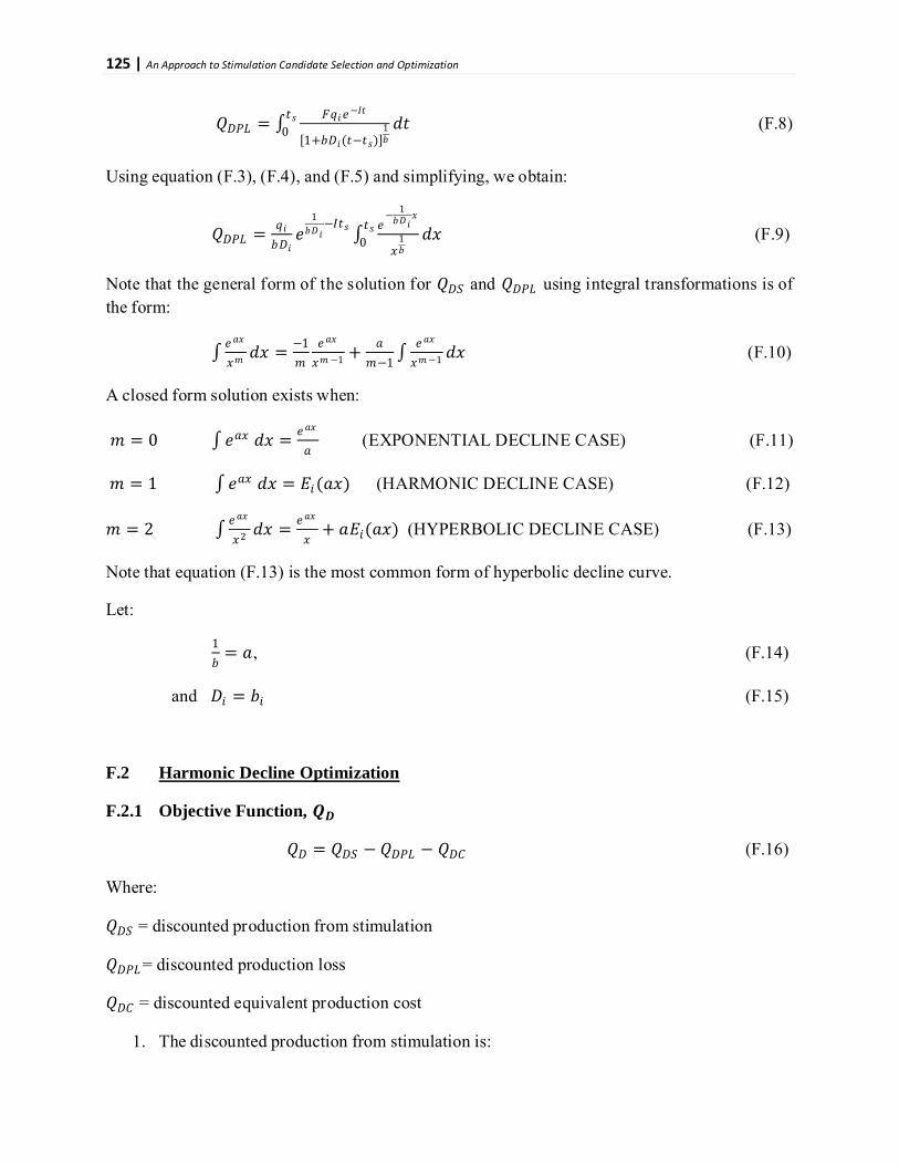
125 | An Approach to Stimulation Candidate Selection and Optimization
𝑄𝑄𝐷𝐷𝐷𝐷𝐷𝐷 = ∫ 𝐹𝐹𝑞𝑞𝑖𝑖𝑒𝑒−𝐼𝐼𝑡𝑡
[1+𝑏𝑏𝐷𝐷𝑖𝑖(𝑡𝑡−𝑡𝑡𝑠𝑠)]1𝑏𝑏
𝑡𝑡𝑠𝑠0 𝑑𝑑𝑡𝑡 (F.8)
Using equation (F.3), (F.4), and (F.5) and simplifying, we obtain:
𝑄𝑄𝐷𝐷𝐷𝐷𝐷𝐷 = 𝑞𝑞𝑖𝑖𝑏𝑏𝐷𝐷𝑖𝑖
𝑒𝑒1
𝑏𝑏𝐷𝐷𝑖𝑖−𝐼𝐼𝑡𝑡𝑠𝑠 ∫ 𝑒𝑒
− 1𝑏𝑏𝐷𝐷𝑖𝑖
𝑥𝑥
𝑥𝑥1𝑏𝑏
𝑡𝑡𝑠𝑠0 𝑑𝑑𝑥𝑥 (F.9)
Note that the general form of the solution for 𝑄𝑄𝐷𝐷𝐷𝐷 and 𝑄𝑄𝐷𝐷𝐷𝐷𝐷𝐷 using integral transformations is of the form:
∫ 𝑒𝑒𝑎𝑎𝑥𝑥
𝑥𝑥𝑚𝑚𝑑𝑑𝑥𝑥 = −1
𝑚𝑚𝑒𝑒𝑎𝑎𝑥𝑥
𝑥𝑥𝑚𝑚−1 + 𝑎𝑎𝑚𝑚−1 ∫
𝑒𝑒𝑎𝑎𝑥𝑥
𝑥𝑥𝑚𝑚−1 𝑑𝑑𝑥𝑥 (F.10)
A closed form solution exists when:
𝑚𝑚 = 0 ∫ 𝑒𝑒𝑎𝑎𝑥𝑥 𝑑𝑑𝑥𝑥 = 𝑒𝑒𝑎𝑎𝑥𝑥
𝑎𝑎 (EXPONENTIAL DECLINE CASE) (F.11)
𝑚𝑚 = 1 ∫ 𝑒𝑒𝑎𝑎𝑥𝑥 𝑑𝑑𝑥𝑥 = 𝐸𝐸𝑖𝑖(𝑎𝑎𝑥𝑥) (HARMONIC DECLINE CASE) (F.12)
𝑚𝑚 = 2 ∫ 𝑒𝑒𝑎𝑎𝑥𝑥
𝑥𝑥2 𝑑𝑑𝑥𝑥 = 𝑒𝑒𝑎𝑎𝑥𝑥
𝑥𝑥+ 𝑎𝑎𝐸𝐸𝑖𝑖(𝑎𝑎𝑥𝑥) (HYPERBOLIC DECLINE CASE) (F.13)
Note that equation (F.13) is the most common form of hyperbolic decline curve.
Let:
1𝑏𝑏
= 𝑎𝑎, (F.14)
and 𝐷𝐷𝑖𝑖 = 𝑏𝑏𝑖𝑖 (F.15)
F.2
F.2.1 Objective Function, 𝑸𝑸𝑫𝑫
Harmonic Decline Optimization
𝑄𝑄𝐷𝐷 = 𝑄𝑄𝐷𝐷𝐷𝐷 − 𝑄𝑄𝐷𝐷𝐷𝐷𝐷𝐷 − 𝑄𝑄𝐷𝐷𝐷𝐷 (F.16)
Where:
𝑄𝑄𝐷𝐷𝐷𝐷 = discounted production from stimulation
𝑄𝑄𝐷𝐷𝐷𝐷𝐷𝐷= discounted production loss
𝑄𝑄𝐷𝐷𝐷𝐷 = discounted equivalent production cost
1. The discounted production from stimulation is:
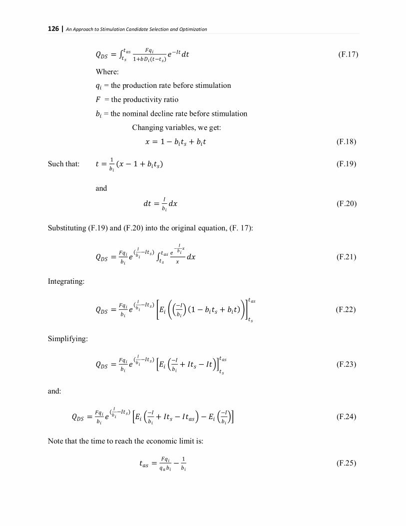
126 | An Approach to Stimulation Candidate Selection and Optimization
𝑄𝑄𝐷𝐷𝐷𝐷 = ∫ 𝐹𝐹𝑞𝑞𝑖𝑖1+𝑏𝑏𝐷𝐷𝑖𝑖(𝑡𝑡−𝑡𝑡𝑠𝑠)
𝑡𝑡𝑎𝑎𝑠𝑠𝑡𝑡𝑠𝑠
𝑒𝑒−𝐼𝐼𝑡𝑡𝑑𝑑𝑡𝑡 (F.17)
Where:
𝑞𝑞𝑖𝑖 = the production rate before stimulation
𝐹𝐹 = the productivity ratio
𝑏𝑏𝑖𝑖 = the nominal decline rate before stimulation
Changing variables, we get:
𝑥𝑥 = 1− 𝑏𝑏𝑖𝑖𝑡𝑡𝑠𝑠 + 𝑏𝑏𝑖𝑖𝑡𝑡 (F.18)
Such that: 𝑡𝑡 = 1𝑏𝑏𝑖𝑖
(𝑥𝑥 − 1 + 𝑏𝑏𝑖𝑖𝑡𝑡𝑠𝑠) (F.19)
and
𝑑𝑑𝑡𝑡 = 𝐼𝐼𝑏𝑏𝑖𝑖𝑑𝑑𝑥𝑥 (F.20)
Substituting (F.19) and (F.20) into the original equation, (F. 17):
𝑄𝑄𝐷𝐷𝐷𝐷 = 𝐹𝐹𝑞𝑞𝑖𝑖𝑏𝑏𝑖𝑖𝑒𝑒
( 𝐼𝐼𝑏𝑏𝑖𝑖−𝐼𝐼𝑡𝑡𝑠𝑠)
∫ 𝑒𝑒− 𝐼𝐼𝑏𝑏𝑖𝑖𝑥𝑥
𝑥𝑥𝑡𝑡𝑎𝑎𝑠𝑠𝑡𝑡𝑠𝑠
𝑑𝑑𝑥𝑥 (F.21)
Integrating:
𝑄𝑄𝐷𝐷𝐷𝐷 = 𝐹𝐹𝑞𝑞𝑖𝑖𝑏𝑏𝑖𝑖𝑒𝑒
( 𝐼𝐼𝑏𝑏𝑖𝑖−𝐼𝐼𝑡𝑡𝑠𝑠)
�𝐸𝐸𝑖𝑖 ��−𝐼𝐼𝑏𝑏𝑖𝑖� (1 − 𝑏𝑏𝑖𝑖𝑡𝑡𝑠𝑠 + 𝑏𝑏𝑖𝑖𝑡𝑡)��
𝑡𝑡𝑠𝑠
𝑡𝑡𝑎𝑎𝑠𝑠 (F.22)
Simplifying:
𝑄𝑄𝐷𝐷𝐷𝐷 = 𝐹𝐹𝑞𝑞𝑖𝑖𝑏𝑏𝑖𝑖𝑒𝑒
( 𝐼𝐼𝑏𝑏𝑖𝑖−𝐼𝐼𝑡𝑡𝑠𝑠)
�𝐸𝐸𝑖𝑖 �−𝐼𝐼𝑏𝑏𝑖𝑖
+ 𝐼𝐼𝑡𝑡𝑠𝑠 − 𝐼𝐼𝑡𝑡��𝑡𝑡𝑠𝑠
𝑡𝑡𝑎𝑎𝑠𝑠 (F.23)
and:
𝑄𝑄𝐷𝐷𝐷𝐷 = 𝐹𝐹𝑞𝑞𝑖𝑖𝑏𝑏𝑖𝑖𝑒𝑒
( 𝐼𝐼𝑏𝑏𝑖𝑖−𝐼𝐼𝑡𝑡𝑠𝑠)
�𝐸𝐸𝑖𝑖 �−𝐼𝐼𝑏𝑏𝑖𝑖
+ 𝐼𝐼𝑡𝑡𝑠𝑠 − 𝐼𝐼𝑡𝑡𝑎𝑎𝑠𝑠� − 𝐸𝐸𝑖𝑖 �−𝐼𝐼𝑏𝑏𝑖𝑖�� (F.24)
Note that the time to reach the economic limit is:
𝑡𝑡𝑎𝑎𝑠𝑠 = 𝐹𝐹𝑞𝑞𝑖𝑖𝑞𝑞𝑎𝑎𝑏𝑏𝑖𝑖
− 1𝑏𝑏𝑖𝑖
(F.25)

127 | An Approach to Stimulation Candidate Selection and Optimization
Where:
𝑞𝑞𝑎𝑎 = abandonment production rate
Therefore equation (F.24) becomes:
𝑄𝑄𝐷𝐷𝐷𝐷 = 𝐹𝐹𝑞𝑞𝑖𝑖𝑏𝑏𝑖𝑖𝑒𝑒
( 1𝑏𝑏𝑖𝑖−𝐼𝐼𝑡𝑡𝑠𝑠)
�𝐸𝐸𝑖𝑖 �𝐼𝐼𝑡𝑡𝑠𝑠 −𝐼𝐼𝐹𝐹𝑞𝑞𝑖𝑖𝑞𝑞𝑎𝑎𝑏𝑏𝑖𝑖
� − 𝐸𝐸𝑖𝑖 �−1𝑏𝑏𝑖𝑖�� (F.26)
2. The discounted production lost during stimulation is:
𝑄𝑄𝐷𝐷𝐷𝐷𝐷𝐷 = ∫ 𝑞𝑞𝑖𝑖𝑒𝑒−𝐼𝐼𝑡𝑡
1+𝑏𝑏𝑖𝑖𝑡𝑡𝑡𝑡𝑠𝑠
0 𝑑𝑑𝑡𝑡 (F.27)
Using the same change of variable:
𝑥𝑥 = 1− 𝑏𝑏𝑖𝑖𝑡𝑡𝑠𝑠 + 𝑏𝑏𝑖𝑖𝑡𝑡 (F.18)
Such that: 𝑡𝑡 = 1𝑏𝑏𝑖𝑖
(𝑥𝑥 − 1 + 𝑏𝑏𝑖𝑖𝑡𝑡𝑠𝑠) (F.19)
and
𝑑𝑑𝑡𝑡 = 1𝑏𝑏𝑖𝑖𝑑𝑑𝑥𝑥 (F.20)
We get:
𝑄𝑄𝐷𝐷𝐷𝐷𝐷𝐷 = 𝑞𝑞𝑖𝑖𝑏𝑏𝑖𝑖𝑒𝑒
1𝑏𝑏𝑖𝑖 ∫ 𝑒𝑒
− 𝐼𝐼𝑏𝑏𝑖𝑖𝑥𝑥
𝑥𝑥𝑡𝑡𝑠𝑠
0 𝑑𝑑𝑥𝑥 (F.28)
and
𝑄𝑄𝐷𝐷𝐷𝐷𝐷𝐷 = 𝑞𝑞𝑖𝑖𝑏𝑏𝑖𝑖𝑒𝑒
𝐼𝐼𝑏𝑏𝑖𝑖 �𝐸𝐸𝑖𝑖 �
−𝐼𝐼𝑏𝑏𝑖𝑖� (1 + 𝑏𝑏𝑖𝑖𝑡𝑡)�
0
𝑡𝑡𝑠𝑠 (F.29)
Therefore:
𝑄𝑄𝐷𝐷𝐷𝐷𝐷𝐷 = 𝑞𝑞𝑖𝑖𝑏𝑏𝑖𝑖𝑒𝑒
𝐼𝐼𝑏𝑏𝑖𝑖 �𝐸𝐸𝑖𝑖 �
−𝐼𝐼𝑏𝑏𝑖𝑖−𝐼𝐼𝑡𝑡𝑠𝑠��
0
𝑡𝑡𝑠𝑠 (F.30)
𝑄𝑄𝐷𝐷𝐷𝐷𝐷𝐷 = 𝑞𝑞𝑖𝑖𝑏𝑏𝑖𝑖𝑒𝑒
𝐼𝐼𝑏𝑏𝑖𝑖 �𝐸𝐸𝑖𝑖 �
−𝐼𝐼𝑏𝑏𝑖𝑖−𝐼𝐼𝑡𝑡𝑠𝑠� − 𝐸𝐸𝑖𝑖 �
−𝐼𝐼𝑏𝑏𝑖𝑖�� (F.31)
3. The discounted equivalent production from stimulation cost is:
𝑄𝑄𝐷𝐷𝐷𝐷 = 𝐷𝐷𝐷𝐷𝑒𝑒−𝐼𝐼𝑡𝑡𝑠𝑠 (F.32)
With the above derivations, 𝑄𝑄𝐷𝐷 can now be written as:
𝑄𝑄𝐷𝐷 = 𝛽𝛽1𝐸𝐸𝑖𝑖(𝛽𝛽2 − 𝛽𝛽3𝐹𝐹)𝐹𝐹 − 𝛽𝛽1𝐸𝐸𝑖𝑖(𝛽𝛽4)𝐹𝐹 − 𝛽𝛽6𝐷𝐷 − 𝛽𝛽5 (F.33)
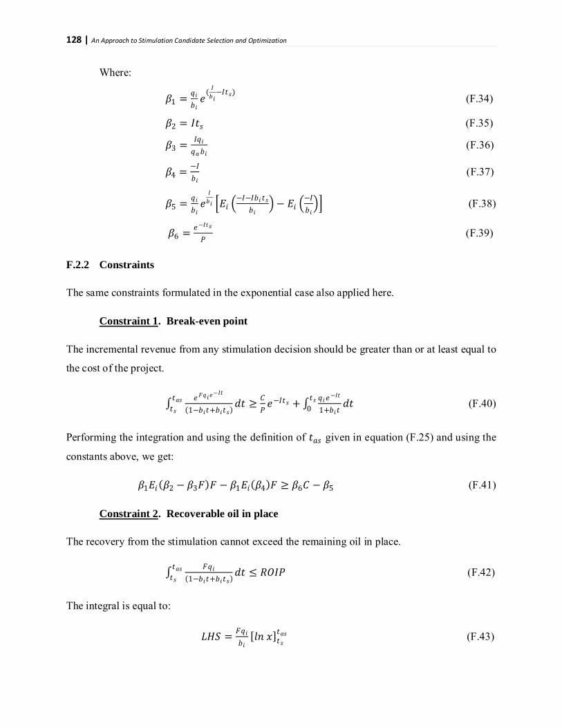
128 | An Approach to Stimulation Candidate Selection and Optimization
Where:
𝛽𝛽1 = 𝑞𝑞𝑖𝑖𝑏𝑏𝑖𝑖𝑒𝑒
( 𝐼𝐼𝑏𝑏𝑖𝑖−𝐼𝐼𝑡𝑡𝑠𝑠)
(F.34)
𝛽𝛽2 = 𝐼𝐼𝑡𝑡𝑠𝑠 (F.35)
𝛽𝛽3 = 𝐼𝐼𝑞𝑞𝑖𝑖𝑞𝑞𝑎𝑎𝑏𝑏𝑖𝑖
(F.36)
𝛽𝛽4 = −𝐼𝐼𝑏𝑏𝑖𝑖
(F.37)
𝛽𝛽5 = 𝑞𝑞𝑖𝑖𝑏𝑏𝑖𝑖𝑒𝑒
𝐼𝐼𝑏𝑏𝑖𝑖 �𝐸𝐸𝑖𝑖 �
−𝐼𝐼−𝐼𝐼𝑏𝑏𝑖𝑖 𝑡𝑡𝑠𝑠𝑏𝑏𝑖𝑖
� − 𝐸𝐸𝑖𝑖 �−𝐼𝐼𝑏𝑏𝑖𝑖�� (F.38)
𝛽𝛽6 = 𝑒𝑒−𝐼𝐼𝑡𝑡𝑠𝑠
𝐷𝐷 (F.39)
F.2.2 Constraints
The same constraints formulated in the exponential case also applied here.
Constraint 1
The incremental revenue from any stimulation decision should be greater than or at least equal to
the cost of the project.
. Break-even point
∫ 𝑒𝑒𝐹𝐹𝑞𝑞𝑖𝑖𝑒𝑒−𝐼𝐼𝑡𝑡
(1−𝑏𝑏𝑖𝑖𝑡𝑡+𝑏𝑏𝑖𝑖𝑡𝑡𝑠𝑠)𝑡𝑡𝑎𝑎𝑠𝑠𝑡𝑡𝑠𝑠
𝑑𝑑𝑡𝑡 ≥ 𝐷𝐷𝐷𝐷𝑒𝑒−𝐼𝐼𝑡𝑡𝑠𝑠 + ∫ 𝑞𝑞𝑖𝑖𝑒𝑒−𝐼𝐼𝑡𝑡
1+𝑏𝑏𝑖𝑖𝑡𝑡𝑡𝑡𝑠𝑠
0 𝑑𝑑𝑡𝑡 (F.40)
Performing the integration and using the definition of 𝑡𝑡𝑎𝑎𝑠𝑠 given in equation (F.25) and using the
constants above, we get:
𝛽𝛽1𝐸𝐸𝑖𝑖(𝛽𝛽2 − 𝛽𝛽3𝐹𝐹)𝐹𝐹 − 𝛽𝛽1𝐸𝐸𝑖𝑖(𝛽𝛽4)𝐹𝐹 ≥ 𝛽𝛽6𝐷𝐷 − 𝛽𝛽5 (F.41)
Constraint 2
The recovery from the stimulation cannot exceed the remaining oil in place.
. Recoverable oil in place
∫ 𝐹𝐹𝑞𝑞𝑖𝑖(1−𝑏𝑏𝑖𝑖𝑡𝑡+𝑏𝑏𝑖𝑖𝑡𝑡𝑠𝑠)
𝑡𝑡𝑎𝑎𝑠𝑠𝑡𝑡𝑠𝑠
𝑑𝑑𝑡𝑡 ≤ 𝑅𝑅𝑅𝑅𝐼𝐼𝐷𝐷 (F.42)
The integral is equal to:
𝐷𝐷𝐿𝐿𝐷𝐷 = 𝐹𝐹𝑞𝑞𝑖𝑖𝑏𝑏𝑖𝑖
[𝑙𝑙𝑙𝑙 𝑥𝑥]𝑡𝑡𝑠𝑠𝑡𝑡𝑎𝑎𝑠𝑠 (F.43)

129 | An Approach to Stimulation Candidate Selection and Optimization
Using the definition of 𝑡𝑡𝑎𝑎𝑠𝑠 and substituting in the equation:
𝐹𝐹𝑞𝑞𝑖𝑖𝑏𝑏𝑖𝑖
ln �𝐹𝐹𝑞𝑞𝑖𝑖−𝑞𝑞𝑎𝑎𝑞𝑞𝑎𝑎𝑏𝑏𝑖𝑖
� − 𝐹𝐹𝑞𝑞𝑖𝑖𝑏𝑏𝑖𝑖𝑙𝑙𝑙𝑙 𝑡𝑡𝑠𝑠 ≤ 𝑅𝑅𝑅𝑅𝐼𝐼𝐷𝐷 (F.44)
and:
𝛽𝛽7𝑙𝑙𝑙𝑙(𝛽𝛽8 − 𝛽𝛽9)𝐹𝐹 − 𝛽𝛽10 ≤ 𝑅𝑅𝑅𝑅𝐼𝐼𝐷𝐷 (F.45)
where:
𝛽𝛽7 = 𝑞𝑞𝑖𝑖𝑏𝑏𝑖𝑖
(F.46)
𝛽𝛽8 = 𝑞𝑞𝑖𝑖𝑞𝑞𝑎𝑎𝑏𝑏𝑖𝑖
(F.47)
𝛽𝛽9 = 1𝑏𝑏𝑖𝑖
(F.48)
𝛽𝛽10 = 𝑞𝑞𝑖𝑖𝑏𝑏𝑖𝑖𝑙𝑙𝑙𝑙 𝑡𝑡𝑠𝑠 (F.49)
Constraint 3
The pr oduction r ate a fter s timulation should n ot e xceed the maximum d esign capacity o f t he
flow string, i.e.,
. Flow string capacity
𝐹𝐹 ≤ 𝑞𝑞𝑚𝑚𝑎𝑎𝑥𝑥𝑞𝑞𝑜𝑜
(F.50)
Where 𝑞𝑞𝑚𝑚𝑎𝑎𝑥𝑥 is the maximum design capacity of the flowing string.
Constraint 4
The cost of the stimulation should not exceed the budget.
. Budget limitation
𝐷𝐷 ≤ 𝐷𝐷𝑚𝑚𝑎𝑎𝑥𝑥 (F.51)
Where 𝐷𝐷𝑚𝑚𝑎𝑎𝑥𝑥 is the budget for the stimulation job.
Constraint 5. Reservoir productivity ratio constraint

130 | An Approach to Stimulation Candidate Selection and Optimization
The maximum attainable pr oductivity ratio from stimulation depends on t he reservoir pr operties
and treatment parameters.
𝐹𝐹 ≤ 𝐹𝐹𝑚𝑚𝑎𝑎𝑥𝑥 (F.52)
Where 𝐹𝐹𝑚𝑚𝑎𝑎𝑥𝑥 is the maximum attainable productivity ratio.
Constraint 6
The cost and productivity ratio relationship can be formulated into the following equation.
. Cost productivity ratio equation
𝐷𝐷 = 10𝑏𝑏0𝐹𝐹𝑏𝑏1 (F.53)
Where 𝑏𝑏0 and 𝑏𝑏1 are the intercept and slope of a regression line through the data.
F.2.3 Form of the NLP
Equations (F.33) and (F.53) define the NLP model for the harmonic case.
Maximize:
𝑄𝑄𝐷𝐷 = 𝛽𝛽1𝐸𝐸𝑖𝑖(𝛽𝛽2 − 𝛽𝛽3𝐹𝐹)𝐹𝐹 − 𝛽𝛽1𝐸𝐸𝑖𝑖(𝛽𝛽4)𝐹𝐹 − 𝛽𝛽6𝐷𝐷 − 𝛽𝛽5 (F.33)
Subject to:
𝛽𝛽1𝐸𝐸𝑖𝑖(𝛽𝛽2 − 𝛽𝛽3𝐹𝐹)𝐹𝐹 − 𝛽𝛽1𝐸𝐸𝑖𝑖(𝛽𝛽4)𝐹𝐹 ≥ 𝛽𝛽6𝐷𝐷 − 𝛽𝛽5 (F.41)
𝛽𝛽7𝑙𝑙𝑙𝑙(𝛽𝛽8 − 𝛽𝛽9)𝐹𝐹 − 𝛽𝛽10 ≤ 𝑅𝑅𝑅𝑅𝐼𝐼𝐷𝐷 (F.45)
𝐹𝐹 ≤ 𝑞𝑞𝑚𝑚𝑎𝑎𝑥𝑥𝑞𝑞𝑜𝑜
(F.50)
𝐷𝐷 ≤ 𝐷𝐷𝑚𝑚𝑎𝑎𝑥𝑥 (F.51)
𝐹𝐹 ≤ 𝐹𝐹𝑚𝑚𝑎𝑎𝑥𝑥 (F.52)
𝐷𝐷 = 10𝑏𝑏0𝐹𝐹𝑏𝑏1 (F.53)

131 | An Approach to Stimulation Candidate Selection and Optimization
To develop a closed form solution to the model, we shall consider only the case when 𝑚𝑚 = 2.
The solution form to the general case is given in equation (F.13).
F.3 Hyperbolic Decline Optimization
F.3.1 Objective Function, 𝑸𝑸𝑫𝑫
The objective function is formulated as:
𝑄𝑄𝐷𝐷 = 𝑄𝑄𝐷𝐷𝐷𝐷 − 𝑄𝑄𝐷𝐷𝐷𝐷𝐷𝐷 − 𝑄𝑄𝐷𝐷𝐷𝐷 (F.16)
Where:
𝑄𝑄𝐷𝐷𝐷𝐷 = discounted production from stimulation
𝑄𝑄𝐷𝐷𝐷𝐷𝐷𝐷= discounted production loss
𝑄𝑄𝐷𝐷𝐷𝐷 = discounted equivalent production cost
1. The discounted production from stimulation is:
𝑄𝑄𝐷𝐷𝐷𝐷 = ∫ 𝐹𝐹𝑞𝑞𝑖𝑖
�1+𝑏𝑏𝑖𝑖2 (𝑡𝑡−𝑡𝑡𝑠𝑠)�
2𝑡𝑡𝑎𝑎𝑠𝑠𝑡𝑡𝑠𝑠
𝑒𝑒−𝐼𝐼𝑡𝑡𝑑𝑑𝑡𝑡 (F.54)
Changing variables, we get:
𝑥𝑥 = 1− 𝑏𝑏𝑖𝑖2𝑡𝑡𝑠𝑠 + 𝑏𝑏𝑖𝑖
2𝑡𝑡 (F.55)
Such that:
𝑡𝑡 = 2𝑏𝑏𝑖𝑖
(𝑥𝑥 − 1 + 𝑏𝑏𝑖𝑖2𝑡𝑡𝑠𝑠) (F.56)
and
𝑑𝑑𝑡𝑡 = 2𝑏𝑏𝑖𝑖𝑑𝑑𝑥𝑥 (F.57)
Substituting equations (F.55), (F.56) and (F.57) into (F. 54), then simplifying:
𝑄𝑄𝐷𝐷𝐷𝐷 = 2𝐹𝐹𝑞𝑞𝑖𝑖𝑏𝑏𝑖𝑖
𝑒𝑒�2𝐼𝐼𝑏𝑏𝑖𝑖−𝐼𝐼𝑡𝑡𝑠𝑠� ∫ 𝑒𝑒
−2𝐼𝐼𝑏𝑏𝑖𝑖𝑥𝑥
𝑥𝑥2𝑡𝑡𝑎𝑎𝑠𝑠𝑡𝑡𝑠𝑠
𝑑𝑑𝑥𝑥 (F.58)

132 | An Approach to Stimulation Candidate Selection and Optimization
The economic life is:
𝑡𝑡𝑎𝑎𝑠𝑠 = 2𝑏𝑏𝑖𝑖�𝐹𝐹𝑞𝑞𝑖𝑖𝑞𝑞𝑎𝑎�
0.5− 2
𝑏𝑏𝑖𝑖 (F.59)
Integrating equation (F.58), then substituting equation (F.59) and simplifying:
𝑄𝑄𝐷𝐷𝐷𝐷 = −𝜖𝜖3𝑒𝑒𝐼𝐼𝑡𝑡𝑠𝑠−
2𝑏𝑏𝑖𝑖�𝐹𝐹𝑞𝑞 𝑖𝑖𝑞𝑞𝑎𝑎
�0.5
𝐹𝐹
−𝑏𝑏𝑖𝑖2 𝑡𝑡𝑠𝑠+�𝐹𝐹𝑞𝑞 𝑖𝑖𝑞𝑞𝑎𝑎�
0.5 + 𝜖𝜖1𝜖𝜖3𝐹𝐹 − 𝜖𝜖2𝜖𝜖3𝐹𝐹 (F.60)
where:
𝜖𝜖1 = �−2𝐼𝐼𝑏𝑏𝑖𝑖� 𝐸𝐸𝑖𝑖 �𝐼𝐼𝑡𝑡𝑠𝑠 −
2𝐼𝐼𝑏𝑏𝑖𝑖�𝐹𝐹𝑞𝑞𝑖𝑖𝑞𝑞𝑎𝑎�
0.5� (F.61)
𝜖𝜖2 = −𝑒𝑒−2𝐼𝐼𝑏𝑏𝑖𝑖 + �−2𝐼𝐼
𝑏𝑏𝑖𝑖� 𝐸𝐸𝑖𝑖 �
−2𝐼𝐼𝑏𝑏𝑖𝑖� (F.62)
𝜖𝜖3 = 2𝑞𝑞𝑖𝑖𝑒𝑒2𝐼𝐼𝑏𝑏𝑖𝑖 𝑒𝑒𝐼𝐼𝑡𝑡𝑠𝑠
𝑏𝑏𝑖𝑖 (F.63)
2. The discounted production lost during stimulation is:
𝑄𝑄𝐷𝐷𝐷𝐷𝐷𝐷 = ∫ 𝑞𝑞𝑖𝑖𝑒𝑒−𝐼𝐼𝑡𝑡
1+𝑏𝑏𝑖𝑖2 𝑡𝑡
𝑡𝑡𝑠𝑠0 𝑑𝑑𝑡𝑡 (F.64)
Using similar variable change and simplifying:
𝑄𝑄𝐷𝐷𝐷𝐷𝐷𝐷 = 2𝑞𝑞𝑖𝑖𝑏𝑏𝑖𝑖𝑒𝑒
2𝐼𝐼𝑏𝑏𝑖𝑖 �−𝑒𝑒
�−2𝐼𝐼𝑏𝑏𝑖𝑖
��1+𝑏𝑏𝑖𝑖2 𝑡𝑡�
�1+𝑏𝑏𝑖𝑖2 𝑡𝑡�
+ �−2𝐼𝐼𝑏𝑏𝑖𝑖� 𝐸𝐸𝑖𝑖 ��
−2𝐼𝐼𝑏𝑏𝑖𝑖� �1 + 𝑏𝑏𝑖𝑖
2𝑡𝑡���
0
𝑡𝑡𝑠𝑠
(F.65)
Simplifying further:
𝑄𝑄𝐷𝐷𝐷𝐷𝐷𝐷 = 2𝑞𝑞𝑖𝑖𝑏𝑏𝑖𝑖𝑒𝑒
2𝐼𝐼𝑏𝑏𝑖𝑖 �−𝑒𝑒
−2𝐼𝐼−𝐼𝐼𝑡𝑡𝑠𝑠
�1+𝑏𝑏𝑖𝑖2 𝑡𝑡𝑠𝑠�
+ �−2𝐼𝐼𝑏𝑏𝑖𝑖�𝐸𝐸𝑖𝑖 �
−2𝐼𝐼𝑏𝑏𝑖𝑖− 𝐼𝐼𝑡𝑡𝑠𝑠� + 𝑒𝑒
−2𝐼𝐼𝑏𝑏𝑖𝑖 + �−2𝐼𝐼
𝑏𝑏𝑖𝑖� 𝐸𝐸𝑖𝑖 �
−2𝐼𝐼𝑏𝑏𝑖𝑖�� (F.66)
This expression for 𝑄𝑄𝐷𝐷𝐷𝐷𝐷𝐷 is constant.

133 | An Approach to Stimulation Candidate Selection and Optimization
We can define:
𝜖𝜖4 = 2𝑞𝑞𝑖𝑖𝑏𝑏𝑖𝑖𝑒𝑒
2𝐼𝐼𝑏𝑏𝑖𝑖 �−𝑒𝑒
−2𝐼𝐼−𝐼𝐼𝑡𝑡𝑠𝑠
�1+𝑏𝑏𝑖𝑖2 𝑡𝑡𝑠𝑠�
+ �−2𝐼𝐼𝑏𝑏𝑖𝑖�𝐸𝐸𝑖𝑖 �
−2𝐼𝐼𝑏𝑏𝑖𝑖− 𝐼𝐼𝑡𝑡𝑠𝑠� + 𝑒𝑒
−2𝐼𝐼𝑏𝑏𝑖𝑖 + �−2𝐼𝐼
𝑏𝑏𝑖𝑖� 𝐸𝐸𝑖𝑖 �
−2𝐼𝐼𝑏𝑏𝑖𝑖�� (F.67)
1. The discounted equivalent production from stimulation cost is:
𝑄𝑄𝐷𝐷𝐷𝐷 = 𝐷𝐷𝐷𝐷𝑒𝑒−𝐼𝐼𝑡𝑡𝑠𝑠 (F.32)
We can define:
𝜖𝜖5 = 𝑒𝑒−𝐼𝐼𝑡𝑡𝑠𝑠
𝐷𝐷 (F.69)
Therefore:
𝑄𝑄𝐷𝐷𝐷𝐷 = 𝜖𝜖5𝐷𝐷 (F.70)
The objective function 𝑄𝑄𝐷𝐷 can now be written as:
𝑄𝑄𝐷𝐷 = −𝜖𝜖3𝑒𝑒𝜖𝜖8𝑒𝑒𝜖𝜖6𝐹𝐹0.5𝐹𝐹𝜖𝜖9 +𝜖𝜖7𝐹𝐹0.5 + 𝜖𝜖1𝜖𝜖3𝐹𝐹 − 𝜖𝜖2𝜖𝜖3𝐹𝐹 − 𝜖𝜖4 − 𝜖𝜖5𝐷𝐷 (F.71)
Where:
𝜖𝜖6 = −2𝐼𝐼𝑏𝑏𝑖𝑖� 𝑞𝑞𝑖𝑖𝑞𝑞𝑎𝑎�
0.5 (F.72)
𝜖𝜖7 = �𝑞𝑞𝑖𝑖𝑞𝑞𝑎𝑎�
0.5 (F.73)
𝜖𝜖8 = 𝐼𝐼𝑡𝑡𝑠𝑠 (F.74)
𝜖𝜖9 = −𝑏𝑏𝑖𝑖𝑡𝑡𝑠𝑠2
(F.75)
F.3.2 Constraints
The same constraints formulation as in previous cases applies here.
Constraint 1
The incremental revenue from any stimulation decision should be greater than or at least equal to
the cost of the project.
. Break-even point

134 | An Approach to Stimulation Candidate Selection and Optimization
∫ 𝐹𝐹𝑞𝑞𝑖𝑖
�1+𝑏𝑏𝑖𝑖2 (𝑡𝑡−𝑡𝑡𝑠𝑠)�
2𝑡𝑡𝑎𝑎𝑠𝑠𝑡𝑡𝑠𝑠
𝑒𝑒−𝐼𝐼𝑡𝑡𝑑𝑑𝑡𝑡 ≥ 𝐷𝐷𝐷𝐷𝑒𝑒−𝐼𝐼𝑡𝑡𝑠𝑠 + ∫ 𝑞𝑞𝑖𝑖𝑒𝑒−𝐼𝐼𝑡𝑡
1+𝑏𝑏𝑖𝑖2 𝑡𝑡
𝑡𝑡𝑠𝑠0 𝑑𝑑𝑡𝑡 (F.76)
Evaluating:
−𝜖𝜖3𝑒𝑒𝐼𝐼𝑡𝑡𝑠𝑠−
2𝐼𝐼𝑏𝑏𝑖𝑖�𝐹𝐹𝑞𝑞 𝑖𝑖𝑞𝑞𝑎𝑎
�0.5
𝐹𝐹−𝑏𝑏𝑖𝑖 𝑡𝑡𝑠𝑠
2 +�𝐹𝐹𝑞𝑞 𝑖𝑖𝑞𝑞𝑎𝑎�
0.5 + 𝜖𝜖1𝜖𝜖3𝐹𝐹 − 𝜖𝜖2𝜖𝜖3𝐹𝐹 ≥ 𝜖𝜖4 + 𝜖𝜖5𝐷𝐷 (F.77)
Constraint 2
The recovery from the stimulation cannot exceed the remaining oil in place.
. Recoverable oil in place
∫ 𝐹𝐹𝑞𝑞𝑖𝑖
�1+𝑏𝑏𝑖𝑖2 (𝑡𝑡−𝑡𝑡𝑠𝑠)�
2𝑡𝑡𝑎𝑎𝑠𝑠𝑡𝑡𝑠𝑠
𝑒𝑒−𝐼𝐼𝑡𝑡𝑑𝑑𝑡𝑡 ≤ 𝑅𝑅𝑅𝑅𝐼𝐼𝐷𝐷 (F.78)
Evaluating the left hand side:
𝐷𝐷𝐿𝐿𝐷𝐷 = 2𝐹𝐹𝑞𝑞𝑖𝑖𝑏𝑏𝑖𝑖
� −1
1+𝑏𝑏𝑖𝑖2 𝑡𝑡−
𝑏𝑏𝑖𝑖2 𝑡𝑡𝑠𝑠�𝑡𝑡𝑠𝑠
𝑡𝑡𝑎𝑎𝑠𝑠 (F.79)
Simplifying using the definition of 𝑡𝑡𝑎𝑎𝑠𝑠 and the defined constants:
𝜖𝜖10𝐹𝐹𝜖𝜖7𝐹𝐹0.5−𝜖𝜖1 1𝜖𝜖7𝐹𝐹0.5−𝜖𝜖9
≤ 𝑅𝑅𝑅𝑅𝐼𝐼𝐷𝐷 (F.80)
Where:
𝜖𝜖10 = 2𝑞𝑞𝑖𝑖𝑏𝑏𝑖𝑖
(F.81)
Constraint 3
The pr oduction r ate a fter stimulation should n ot e xceed t he maximum d esign capacity o f t he
flow string, i.e.,
. Flow string capacity
𝐹𝐹 ≤ 𝑞𝑞𝑚𝑚𝑎𝑎𝑥𝑥𝑞𝑞𝑖𝑖
(F.82)
Where 𝑞𝑞𝑚𝑚𝑎𝑎𝑥𝑥 is the maximum design capacity of the flowing string.
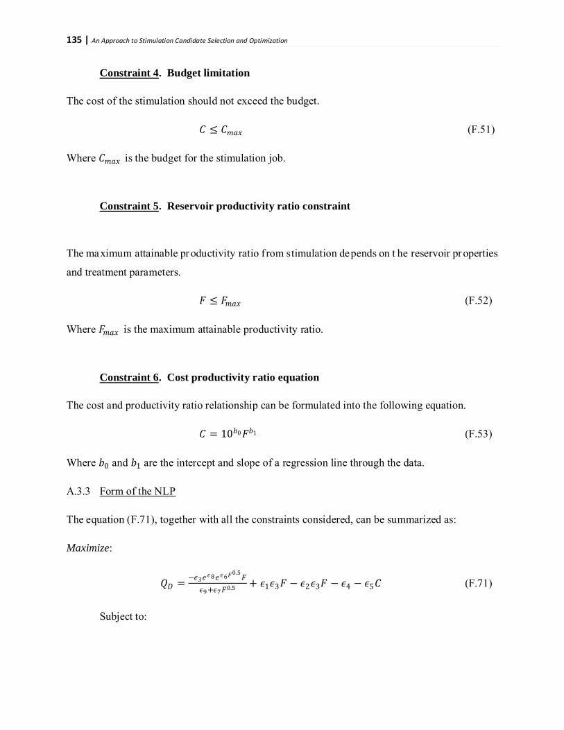
135 | An Approach to Stimulation Candidate Selection and Optimization
Constraint 4
The cost of the stimulation should not exceed the budget.
. Budget limitation
𝐷𝐷 ≤ 𝐷𝐷𝑚𝑚𝑎𝑎𝑥𝑥 (F.51)
Where 𝐷𝐷𝑚𝑚𝑎𝑎𝑥𝑥 is the budget for the stimulation job.
Constraint 5
. Reservoir productivity ratio constraint
The maximum attainable pr oductivity ratio from stimulation depends on t he reservoir pr operties
and treatment parameters.
𝐹𝐹 ≤ 𝐹𝐹𝑚𝑚𝑎𝑎𝑥𝑥 (F.52)
Where 𝐹𝐹𝑚𝑚𝑎𝑎𝑥𝑥 is the maximum attainable productivity ratio.
Constraint 6
The cost and productivity ratio relationship can be formulated into the following equation.
. Cost productivity ratio equation
𝐷𝐷 = 10𝑏𝑏0𝐹𝐹𝑏𝑏1 (F.53)
Where 𝑏𝑏0 and 𝑏𝑏1 are the intercept and slope of a regression line through the data.
A.3.3
The equation (F.71), together with all the constraints considered, can be summarized as:
Form of the NLP
Maximize:
𝑄𝑄𝐷𝐷 = −𝜖𝜖3𝑒𝑒𝜖𝜖8𝑒𝑒𝜖𝜖6𝐹𝐹0.5𝐹𝐹𝜖𝜖9 +𝜖𝜖7𝐹𝐹0.5 + 𝜖𝜖1𝜖𝜖3𝐹𝐹 − 𝜖𝜖2𝜖𝜖3𝐹𝐹 − 𝜖𝜖4 − 𝜖𝜖5𝐷𝐷 (F.71)
Subject to:
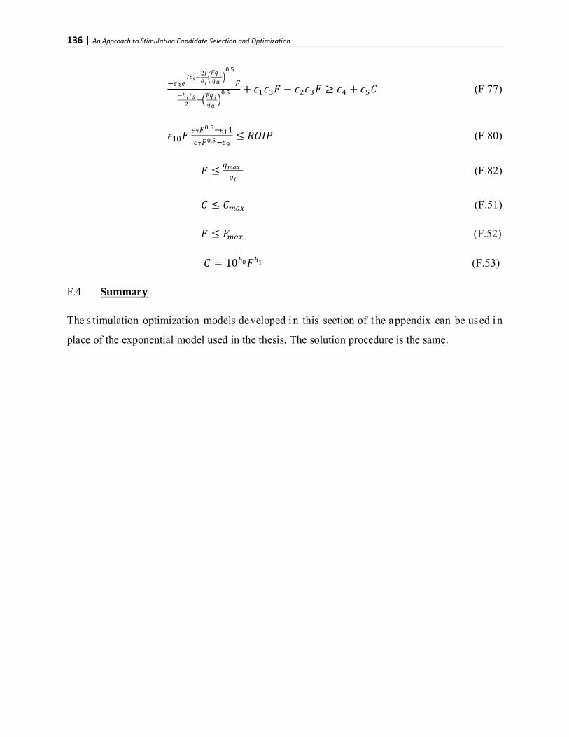
136 | An Approach to Stimulation Candidate Selection and Optimization
−𝜖𝜖3𝑒𝑒𝐼𝐼𝑡𝑡𝑠𝑠−
2𝐼𝐼𝑏𝑏𝑖𝑖�𝐹𝐹𝑞𝑞 𝑖𝑖𝑞𝑞𝑎𝑎
�0.5
𝐹𝐹−𝑏𝑏𝑖𝑖 𝑡𝑡𝑠𝑠
2 +�𝐹𝐹𝑞𝑞 𝑖𝑖𝑞𝑞𝑎𝑎�
0.5 + 𝜖𝜖1𝜖𝜖3𝐹𝐹 − 𝜖𝜖2𝜖𝜖3𝐹𝐹 ≥ 𝜖𝜖4 + 𝜖𝜖5𝐷𝐷 (F.77)
𝜖𝜖10𝐹𝐹𝜖𝜖7𝐹𝐹0.5−𝜖𝜖1 1𝜖𝜖7𝐹𝐹0.5−𝜖𝜖9
≤ 𝑅𝑅𝑅𝑅𝐼𝐼𝐷𝐷 (F.80)
𝐹𝐹 ≤ 𝑞𝑞𝑚𝑚𝑎𝑎𝑥𝑥𝑞𝑞𝑖𝑖
(F.82)
𝐷𝐷 ≤ 𝐷𝐷𝑚𝑚𝑎𝑎𝑥𝑥 (F.51)
𝐹𝐹 ≤ 𝐹𝐹𝑚𝑚𝑎𝑎𝑥𝑥 (F.52)
𝐷𝐷 = 10𝑏𝑏0𝐹𝐹𝑏𝑏1 (F.53)
F.4
The s timulation optimization models developed i n this section of t he appendix can be used i n
place of the exponential model used in the thesis. The solution procedure is the same.
Summary