Embed Size (px)
Citation preview
YICHONG YUN
An Approach to Optimizing the Scheduling of Assembly Lines
Controlled by Web Services
Master’s thesis
Examiner: Professor José Luis Martínez Lastra
Examiner and topic approved by the Faculty
Council of the Faculty of Engineering Sciences
on 5 June, 2013.

I
ABSTRACT
TAMPERE UNIVERSITY OF TECHNOLOGY
Master’s Degree Programme in Machine Automation
Yun,Yichong: An Approach to Optimizing the Scheduling of Assembly Lines
Controlled by Web Services
Master of Science Thesis, 62 pages
June 2014
Major subject: Factory Automation
Examiner: Professor José Luis Martínez Lastra
Keywords: optimization, scheduling, process, production.
The combination of factory automation and computer science plays intense important
role in modern manufacturing business.
This thesis introduces a scheduling & optimization system applied on one assembly
line. The implementation relies on JAVA and Drools rule language. The system is
divided into several small modules including Orders, Facilities and Processes Model
Design, Optimization. The Orders module uses JAXB technology to access and
process an input XML file as the initial order list for scheduling. The Facilities and
Processes Model Design Module uses a tabu search algorithm to retrieve a ’best’
scheduling solution. The Optimization module offers several solutions for the same
optimization constraints, according to the different initial conditions that are input.
The tests were perfomed on a real life assembly line originally used for the assembly
of mobile phones. The approach is representative for customized and modularized
detailed scheduling optimization and could be used for other types of assembly lines as
well.

II
PREFACE
Foremost, I would like to express my sincere gratitude to my supervisor Prof. José Luis
Martínez Lastra for offering me the opportunity to do this topic for master thesis.
I give my appreciates to Corina Postelnicu, thanks for the suggestions of the research
and revision of my thesis writing, for her patience, enthusiasm, and immense
knowledge.
My sincere thanks also go to Luis Gonzalez Moctezuma and Johannes Minor, for
teaching me the use of the system and the knowledge about software development.
Also I thank my friends: Qianting Liu, Yu Guo, Wenxin Zhang, Ana Gomez Espinosa
Martin and Jaime Rubio Nuñez, for the support and comfort when I feel depressed for
the study and life.
Last but not the least, I would like to thank my parents, for the understanding and
supporting me spiritually throughout my life.
Yichong Yun
June 2014
III
Content
1. Introduction ............................................................................................................. 1
1.1 Problem Definition ................................................................................................ 1
1.2 Work Description................................................................................................... 3
1.3 Thesis Outline ....................................................................................................... 4
2. Theoretical Background ......................................................................................... 6
2.1 Planning and Scheduling in Factory Automation ................................................. 6
2.1.1 Factory Automation ....................................................................................... 6
2.1.2 Planning in Factory Automation ................................................................... 9
2.1.3 Scheduling in Factory Automation ............................................................. 10
2.2 Service Oriented Architecture and Web Services ................................................ 11
2.3 Overview of scheduling search algorithms ......................................................... 13
2.3.1 First Fit ........................................................................................................ 14
2.3.2 Local Search ................................................................................................ 16
2.3.3 Tabu Search ................................................................................................. 17
2.4 Scheduling Software ............................................................................................ 18
2.5 ISA 95 Standard .................................................................................................. 19
3. Technical Approach ............................................................................................... 20
3.1 Standard .............................................................................................................. 20
3.2 Technology .......................................................................................................... 21
3.2.1 JAVA............................................................................................................ 21
3.2.2 Referential Software.................................................................................... 22
4. Implementation ..................................................................................................... 26
4.1 Test bed description ............................................................................................. 26
4.2 Software implementation ..................................................................................... 27
4.2.1 Implementation Architecture ....................................................................... 28
4.2.2 Order ........................................................................................................... 33
IV
4.2.3 Application .................................................................................................. 34
4.2.4 Domain ........................................................................................................ 37
4.2.5 Solver .......................................................................................................... 38
5. Results and Discussion .......................................................................................... 43
5.1 Result Presentation ............................................................................................. 44
5.2 Initial scheduling and result comparison ............................................................ 47
6. Conclusions ............................................................................................................ 50
References ...................................................................................................................... 51
Network References ...................................................................................................... 53
V
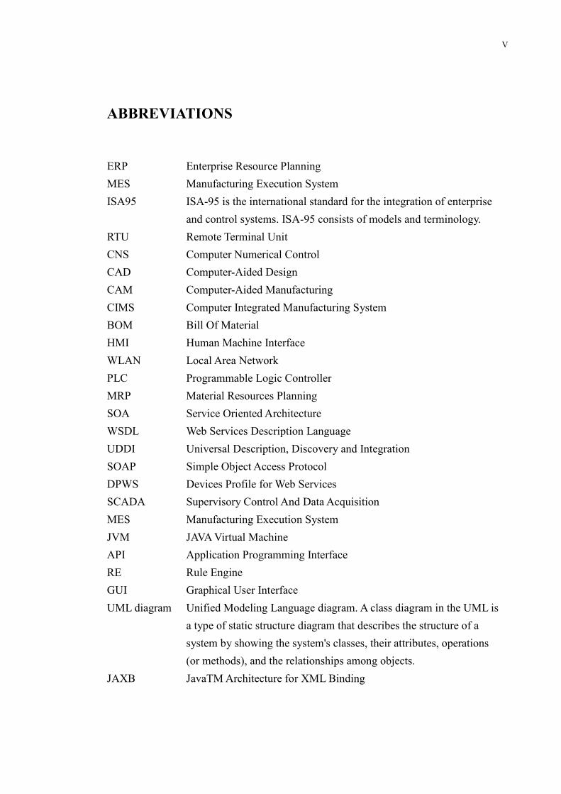
ABBREVIATIONS
ERP Enterprise Resource Planning
MES Manufacturing Execution System
ISA95 ISA-95 is the international standard for the integration of enterprise
and control systems. ISA-95 consists of models and terminology.
RTU Remote Terminal Unit
CNS Computer Numerical Control
CAD Computer-Aided Design
CAM Computer-Aided Manufacturing
CIMS Computer Integrated Manufacturing System
BOM Bill Of Material
HMI Human Machine Interface
WLAN Local Area Network
PLC Programmable Logic Controller
MRP Material Resources Planning
SOA Service Oriented Architecture
WSDL Web Services Description Language
UDDI Universal Description, Discovery and Integration
SOAP Simple Object Access Protocol
DPWS Devices Profile for Web Services
SCADA Supervisory Control And Data Acquisition
MES Manufacturing Execution System
JVM JAVA Virtual Machine
API Application Programming Interface
RE Rule Engine
GUI Graphical User Interface
UML diagram Unified Modeling Language diagram. A class diagram in the UML is
a type of static structure diagram that describes the structure of a
system by showing the system's classes, their attributes, operations
(or methods), and the relationships among objects.
JAXB JavaTM Architecture for XML Binding

VI
FIGURE LIST
Figure 1 Information Flow Diagram in a Manufacturing System............................. 2
Figure 2 Diagram of System Architecture ................................................................ 4
Figure 3 Architecture of ERP System. ...................................................................... 7
Figure 4 Automation Production Line of Tesla Automotive. .................................... 8
Figure 5 Factory Automation System levels. ............................................................ 9
Figure 6 the overview of Material Requirements Planning system. ....................... 10
Figure 7 Architecture of Web Service. .................................................................... 12
Figure 8 Room arrangement problem using first fit and first fit decreasing
algorithms. ....................................................................................................... 15
Figure 9 Function Classification. ............................................................................ 19
Figure 10 Functional Model of Business and Control. ........................................... 21
Figure 11 Screen shots for Drools planner GUI. ..................................................... 25
Figure 12 Physical layout of assembly line............................................................. 26
Figure 13 System Communication Architecture. .................................................... 27
Figure 14 Diagram of Scheduling System. ............................................................. 28
Figure 15 Program Schema of System. ................................................................... 29
Figure 16 UML Class Model of Package Order. ..................................................... 30
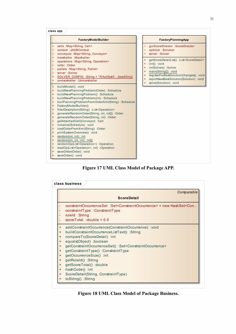
Figure 17 UML Class Model of Package APP. ....................................................... 31
Figure 18 UML Class Model of Package Business. ................................................ 31
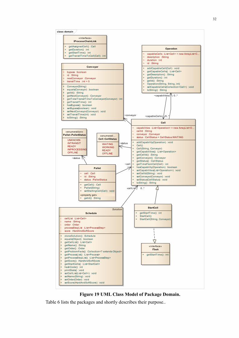
Figure 19 UML Class Model of Package Domain. ................................................. 32
Figure 20 Part of XML Raw Order Files. ............................................................... 33
Figure 21 Output Detail Process Order. .................................................................. 34
Figure 22 Architecture of Solver System. ............................................................... 38
Figure 23 Configuration file in Solver package. ..................................................... 39
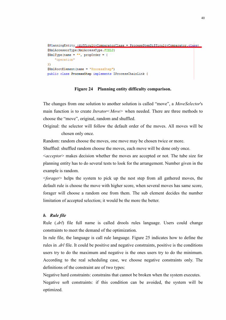
Figure 24 Planning entity difficulty comparison. ................................................... 40
Figure 25 Constraints definition parts of rule file. .................................................. 41
Figure 26 Code for score calculation in drools rule language file. ......................... 42
Figure 27 Software running processes. ................................................................... 43
Figure 28 Cell Usage Percentage in Optimization. ................................................. 48
VII
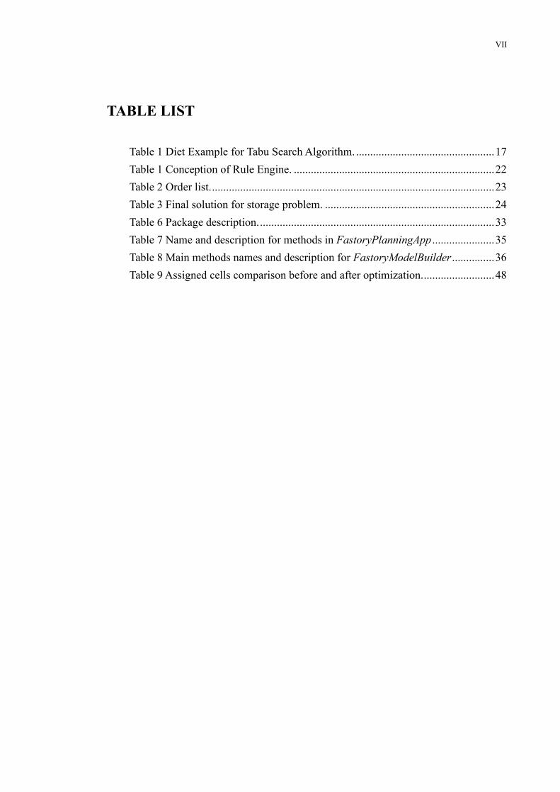
TABLE LIST
Table 1 Diet Example for Tabu Search Algorithm. ................................................. 17
Table 1 Conception of Rule Engine. ....................................................................... 22
Table 2 Order list. .................................................................................................... 23
Table 3 Final solution for storage problem. ............................................................ 24
Table 6 Package description. ................................................................................... 33
Table 7 Name and description for methods in FastoryPlanningApp ...................... 35
Table 8 Main methods names and description for FastoryModelBuilder ............... 36
Table 9 Assigned cells comparison before and after optimization. ......................... 48
1
1. Introduction
1.1 Problem Definition
In industry scheduling (Pinedo, 2005) refers to the reasonable arrangement of
production processes. Three questions are of interest when scheduling:
� “when?”, i.e. the time to load the production materials and to do the processes
� “where?”, i.e. the place that the product is going to be made; and
� “how?”, i.e. the species of products and detail process steps.
Scheduling may focus on either one or all levels of ISA95 (ANSI/ISA–95.00.01–2000,
2000), Enterprise Resource Planning (ERP), Manufacturing Execution System (MES)
or the shop floor. Shop floor scheduling targets detailed short term production (days,
hours), guiding the sequencing of operations, allocation of resources, jobs and
machines to the shop floor , while interacting with long-term enterprise production
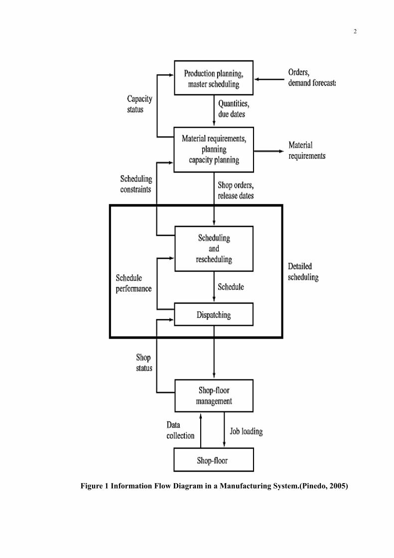
planning, taking the firm’s overall cost and benefits into consideration. Figure 1
illustrates the information flow generally associated with planning and scheduling in a
manufacturing system:
2
Figure 1 Information Flow Diagram in a Manufacturing System.(Pinedo, 2005)
3
Orders / demand forecast is input to a master scheduling system to generate production
quantities and due date; based on this data, companies become aware of manufacturing
capacity, take decisions concerning materials and give shop order / release date to the
downstream manufacturers. A Production Dispatcher module, at the shop floor,
executes the dictated scheduling processes. Feedback is given at all times to the
upstream equipment.
1.2 Work Description
The aim of this work is to develop a flexible optimizing scheduling system for an
automatic production line. Prior to incorporating the scheduling system to line, the
entire production was relying on a simple innelar control system, meaning all materials
would traverse all working cells before production finish. Without the Scheduling
System, the pallets would always choose the nearest working cell for production, often
leaving others completely free. Additionally, with machine breakdowns, the control
system needed to be rewritten , and the production line had to be shut down, thus
extending production cycle and cost.
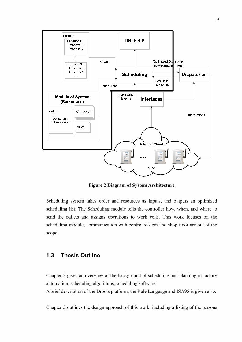
Figure 2 depicts the design of the system. A likely sequencing of operations is
presented as follows:
� The Control module sends requests for scheduling actions .
� The Scheduling module generates an optimization scheduling architecture
based on Drools platform and sends this to the control module.
� The Control module gives instructions to remote terminal units (RTUs) for
detailed control of the work cells and other components.
� The RTUs give feedback or information concerning relevant events to the
Scheduling module – to enable scheduling reactive in case of problems at the
shop floor (e.g. machine breakdown / emergencies)
� Control module – to support production tracking and communication with the
Scheduling module.
4
Figure 2 Diagram of System Architecture
Scheduling system takes order and resources as inputs, and outputs an optimized
scheduling list. The Scheduling module tells the controller how, when, and where to
send the pallets and assigns operations to work cells. This work focuses on the
scheduling module; communication with control system and shop floor are out of the
scope.
1.3 Thesis Outline
Chapter 2 gives an overview of the background of scheduling and planning in factory
automation, scheduling algorithms, scheduling software.
A brief description of the Drools platform, the Rule Language and ISA95 is given also.
Chapter 3 outlines the design approach of this work, including a listing of the reasons

5
for choosing ISA’95 and the scheduling optimization algorithm used.
Chapter 4 gives details on the software implementation.and the test results for a real
assembly line.
Chapter 5 gives a summary and conclusions.
6
2. Theoretical Background
2.1 Planning and Scheduling in Factory Automation
2.1.1 Factory Automation
The 1940s came with increased market demand and higher quality requirement of
products, manufacturers began to give more importance to the full utilization of
resources, while expecting to reduce labor intensity. Single control machines e.g.
Computer Numerical Control (CNSs) replaced manual labor, and gradually became the
main manufacturing unit. (Gongye Zidonghua Jishu He Fazhanshi, 2014)
Starting with the middle of 1960s, a lot of workers lost ground to production line to
ensure large quantities and consistent quality of products. At the same time, the
software for design and development (Computer-Aided Design (CAD),
Computer-Aided Manufacturing (CAM)) came to support product designers.
In 1973 Dr. J. Harrington (WU, Fan, & XIAO, 2014) first proposed the concept of
Computer Integrated Manufacturing System (CIMS): the integration of various
separate parts (CAD/CAM /CAPP/CAQ/FMS) of the enterprise with people through
computer to assist coordination of departments and cooperation to improve
competitiveness and productivity.
1993, American company Gartner Group, Inc. developed Enterprise Resource Planning
(ERP) software (L. Wylie, GartnerGroup, April.1990), which was based on Computer
Integrated Manufacturing System (CIMS). Later, the architecture of this software
developed into a new theory of enterprise management which is still working for
eighty percent of the world's top five hundred enterprises. ERP has the information
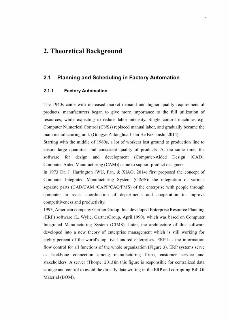
flow control for all functions of the whole organization (Figure 3). ERP systems serve
as backbone connection among manufacturing firms, customer service and
stakeholders. A server (Thorpe, 2013)in this figure is responsible for centralized data
storage and control to avoid the directly data writing in the ERP and corrupting Bill Of
Material (BOM).
7
Figure 3 Architecture of ERP System1.
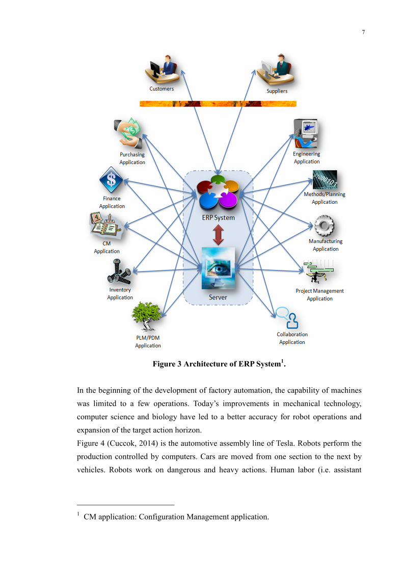
In the beginning of the development of factory automation, the capability of machines
was limited to a few operations. Today’s improvements in mechanical technology,
computer science and biology have led to a better accuracy for robot operations and
expansion of the target action horizon.
Figure 4 (Cuccok, 2014) is the automotive assembly line of Tesla. Robots perform the
production controlled by computers. Cars are moved from one section to the next by
vehicles. Robots work on dangerous and heavy actions. Human labor (i.e. assistant
1 CM application: Configuration Management application.
8
manufacturers) focus on detailed processes that the robots cannot do ( for example,
detail painting, assembly position adjustment).
Figure 4 Automation Production Line of Tesla Automotive.
The architecture of a factory automation system (Figure 5 (Infinion, 2014)) could be
divided into three parts.
� Supervision level - for tracking and monitoring factory systems. The main core
applications are based on PC and operation system (Windows, Linux, etc.);
Human Machine Interface (HMI) can display the status of the system in data or
graphic format to help operators understand the running of production. Wireless
Local Area Network (WLAN) also is able to support this level.
� Control Level - for system execution. HMI, Programmable Logic Controller
(PLC) and field bus are applied in this level for data and massage control.
� Device Level - the lowest field level, includes sensors, actuators, motors .

9
Figure 5 Factory Automation System levels.
2.1.2 Planning in Factory Automation
Production planning is designed before the production to enable the enterprise run in a
long term and make sure the final products are delivered to the customers successfully
and on time. Scheduling refers to the details of the production processes.
Production planning may focus on: enterprise production planning, (including human
resource, finance, logistics) or workshop production planning (of long term production
information for detailed production e.g. resource allocation, product quantities, and due
date, etc.)

10
Starting with the middle of 1960s, manufacturing firms got larger project and orders
from worldwide; simple scheduling could not afford production lines anymore, and
then Material Resources Planning (MRP) developed according to TOYOTA’s “lean
manufacturing philosophy” was applied for planning and scheduling (Hopp &
Spearman, 2004). Figure 5 presents a MRP system architecture. It reveals that, MRP
system is interacted with bills of material (BOM), according to the Order and
Inventory modules, it provides information of master schedule. As introduced for
Figure 1, the master schedule is the input for detail scheduling; it gives the information
about production deadlines to constrain scheduling of details.
Figure 6 the overview of Material Requirements Planning system. (Integrate IT,
2013)
2.1.3 Scheduling in Factory Automation
After First Industry Revolution, machine and new technology took place of handcraft.
The factories were relatively small at that time and produced single products. From
1870s, after Second Industry Revolution, manufacturing firms were able to produce
bulk products and business became worldwide, new technology and theories related to
manufacturing and service came up and formed more systematical business system.

11
Before the limited cost accounting method was published in 1880s, schedules were
very simple specifications of order starts/due date (Herrmann, 2006). Frederick Taylor
(Frederick Winslow Taylor, 2014) separation of planning from execution is seen as the
point zero of modern planning and scheduling, as a separate discipline.
In the 1910s, Henry Laurence Gantt2 published a schedule chart breaking an overall
project period into several elements with detailed timed specifications – the low level
schedules (for batch production), laying the cornerstone for production scheduling. .A
Gantt chart shows all available components for operations, activities needed for
production and set quantities of products on every day depend on previous production
and production ability, during daily production, Gantt chart tracks the production
against the daily goal (Wu, Yushun, & Deyun, 2001).
After Second Industry Revolution, machine replaced human labor to finish the
production, shorter production cycle was not as advantage as before, cost became as
important as time to take into consideration when building schedules. As the goals of
scheduling evolved, different mathematics algorithms have started to apply for the
scheduling problem. And with the development of computer science, scheduling
problem moved to a new era...
Scheduling can be conducted in two ways: statically and dynamically. As the name
says, static scheduling is finished before the production, and it will not change during
manufacturing. This type of scheduling has the problem that when the production has
error or there is machine breakdown, the scheduling planning can not guide the
production anymore and production is interruped. To avoid this problem, dynamic
scheduling uses loop data transfer system to enable reactive scheduling by feedback
information from the control level and shop floor devices.
2.2 Service Oriented Architecture and Web Services
Service Oriented Architecture (SOA) (Service-Oriented Architecture,SOA, 2014). SOA
is an architectural style for software development which is based on the notion of
service3 and network. Services are independent. They have the possibility to finish
2 In (Gantt, 1903), he stated there are two types of balance: “…one of what each
workman should do and did do; the other, of the amount of work to be done and is
done’’ 3 In (Mahmoud, 2005), he mentioned that: “…A service is an implementation of a
well-defined business functionality, and such services can then be consumed by clients
in different applications or business processes.”
12
their own functions and meanwhile they can ensure the other service exchange
information with each other.
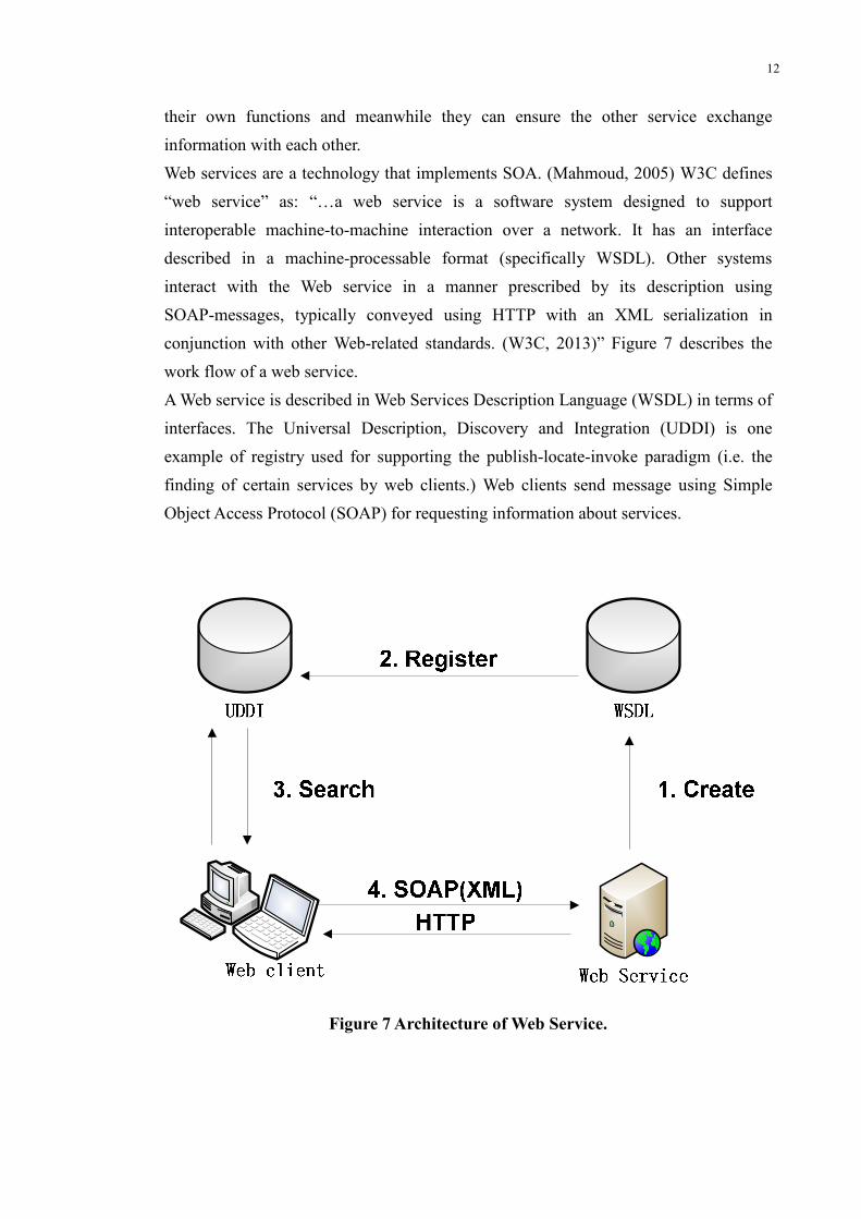
Web services are a technology that implements SOA. (Mahmoud, 2005) W3C defines
“web service” as: “…a web service is a software system designed to support
interoperable machine-to-machine interaction over a network. It has an interface
described in a machine-processable format (specifically WSDL). Other systems
interact with the Web service in a manner prescribed by its description using
SOAP-messages, typically conveyed using HTTP with an XML serialization in
conjunction with other Web-related standards. (W3C, 2013)” Figure 7 describes the
work flow of a web service.
A Web service is described in Web Services Description Language (WSDL) in terms of
interfaces. The Universal Description, Discovery and Integration (UDDI) is one
example of registry used for supporting the publish-locate-invoke paradigm (i.e. the
finding of certain services by web clients.) Web clients send message using Simple
Object Access Protocol (SOAP) for requesting information about services.
Figure 7 Architecture of Web Service.
13
In 2003, the ”SIRENA” project (Service Infrastructure for Real-time Embedded
Networked Applications) (Bohn, Bobek, & Golatowski, 2006) partenered fifteen
companies and universities from three European countries, to build a framework using
a new technology called Devices Profile for Web Services (DPWS) to interconnect
devices in industry, home, vehicle and tecommunication. DPWS enables the devices
communicating with others through network by defining the format and definition of
the technical details of the message transfer. DPWS also shows its cross domain
capability in demonstration, e.g. playing music in a car from home domain using
SIRENA devices by combining usage scenarios, which proved this system
infrastructure could be applied in neworked devices for diverse domains as well. The
further research on devices integration named ”SODA” (Service Oriented
Devices&Delivery Architecture) (Jammes) was aim to develop the inplementation of
DPWS for devices and tools.
In 2006, companies like SAP, Siemens and Schneider Electric joined their efforts in a
European project SOCRADES (Service-Oriented Cross-layer infRAstructure for
Distributed smart Embedded devices) to do further research on the implementation,
and testing of prototypes for DPWS devices based on service oriented architecture in
industry automation domain (Marco, Colombo, & Karnouskos). The test industries
included car engin manufacturing, dynamic assembly system, and cross-enterprise
collaboration in three places. The ArchitecturE for Service-Oriented Process (AESOP)
project (IMC-AESOP Project, 2014), following SOCRADES, focused on merging web
services with Supervisory Control And Data Acquisition (SCADA) system, to realise
more flexibile and economical factory manufacturing.
2.3 Overview of scheduling search algorithms
Algorithm are the backbone of the scheduling optimization problem. This section
provides an overview of scheduling algorithms and their disadvantages and advantages,
with specific focus on the specific algorithms utilized in this work.
There are several types of scheduling algorithms(Bohn et al., 2006):
• Stochastic algorithms based on random functions;
• Heuristic algorithms rely on rules to perform optimization. Such algorithms are
used frequently for dynamic repair. One of the greatest disadvantages of
heuristic algorithms is the fact that the final computed ’best’ solution could be a
local optimal solution instead of the global optimum.
14
• Meta-heuristics algorithms (tabu search, simulated annealing, and genetic
algorithms). These algorithms emerged from heuristic algorithms. The major
difference is that such methods enable the finding of a global ’best’ solution.
• Multi-agent based dynamic algorithms. Such algorithms enable the control by
different agents to avoid long time message transfer between the shop floor and
the scheduling system. Compared to traditional scheduling, which is
single-threaded (leading to one error causing the collapse of a whole system),
multi-agent based dynamic scheduling enables decentralization of control.
The following discussion focuses on the algorithms: First Fit (which is used in the
proposed implementation to generate the initial solution for scheduling
optimization), Local Search and Tabu Search ( which gives the final optimized
schedule proposal).
2.3.1 First Fit
First Fit algorithm is one of the simplest heuristic algorithms to quickly generate a
non-optimized solution. In this work, First Fit is used to generate the initial schedule
for optimization.
Originally, First Fit was applied for the bin packing problem. In bin packing problem,
objects with different loads has to be paced in minimum numbers of bins with same
structure and loads. First fit means the items will be placed in the first bin when it fits.
(Dósa & Sgall, 1998)
First Fit Decreasing algorithm is similar with first fit. The difference consists in the
items having to be sorted in a certain order and then use as first fit.
An illustrated example (Figure 8) is provided as follows, to show both First Fit and
First Fit Decreasing at work.
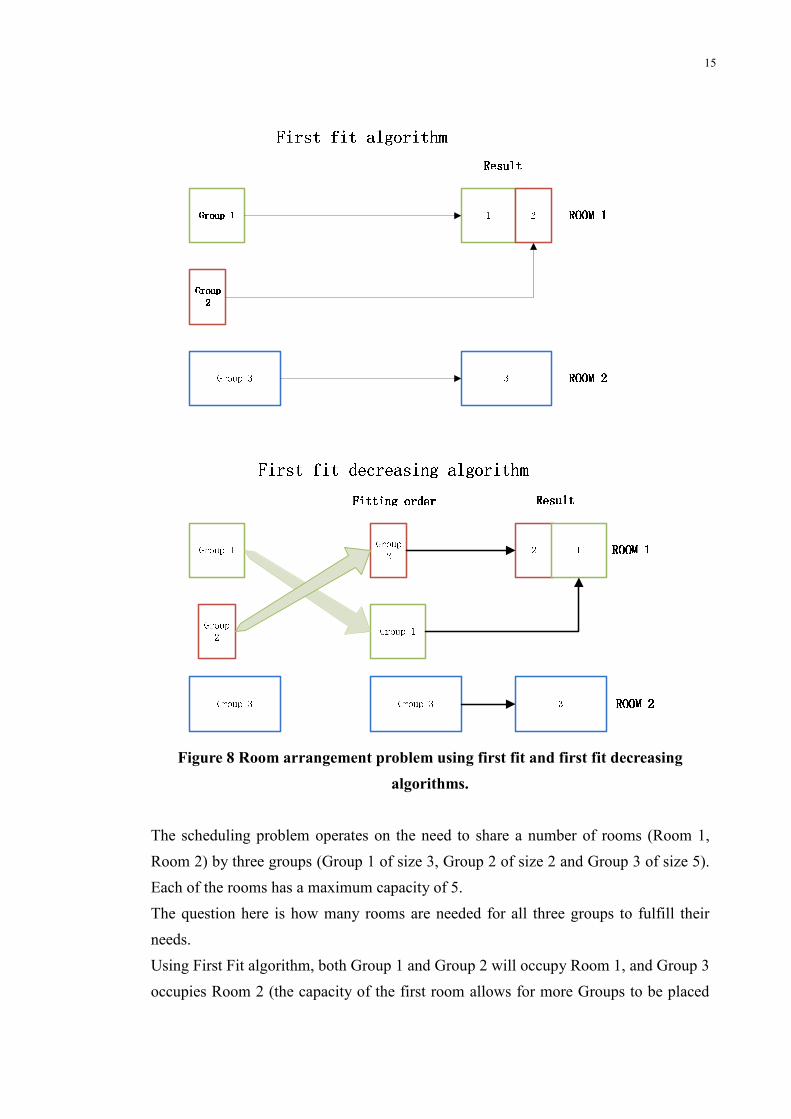
15
Figure 8 Room arrangement problem using first fit and first fit decreasing
algorithms.
The scheduling problem operates on the need to share a number of rooms (Room 1,
Room 2) by three groups (Group 1 of size 3, Group 2 of size 2 and Group 3 of size 5).
Each of the rooms has a maximum capacity of 5.
The question here is how many rooms are needed for all three groups to fulfill their
needs.
Using First Fit algorithm, both Group 1 and Group 2 will occupy Room 1, and Group 3
occupies Room 2 (the capacity of the first room allows for more Groups to be placed
Group Group Group Group 1111Group Group Group Group 2222Fitting orderFitting orderFitting orderFitting order Result Result Result Result ROOM ROOM ROOM ROOM 1111
ROOM ROOM ROOM ROOM 2222
ROOM ROOM ROOM ROOM 1111ROOM ROOM ROOM ROOM 2222
Result Result Result Result
16
there once Group 1 is assigned Room 1, and prevents any further allocations once both
Group 1 and Group 2 are assigned Room 1). So in total there are two rooms needed for
all groups.
First Fit Decreasing sorts all groups decreasingly, based on the number of people in
each group. Therefore, the fitting order is Group 2, then Group 1 and, last, Group 3.
The algorithm for assigning participant groups to each room is the same as the method
used with simple First Fit.
2.3.2 Local Search
Local search gives a fractional solution instead of the best solution. The final solution
is related to the initial value of inputs.
The function frame of local search (Sensen, 2013) is as bellow:
N ≔ number of repetitions;
�̅ ≔ ∅;
��� i = 0 to N
s = initial solution;
����� having a neighbor of s with better solution
$� s ≔ arbitrary neighbor of s with better solution;
�&$ �����
�� s is better than � '
� ' : = �;
end if
�&$ ���
return �̅;
The initial solution is generated randomly, every time a better solution will replace the
previous one for best fit purpose. The advantage of local search is the speedy
computation capability. The final solution is always better than the original (initial)
solution. Disadvantages of local search include the strong dependence on initial
conditions and large number of repetitions (the larger the number, the better the
solution).
17
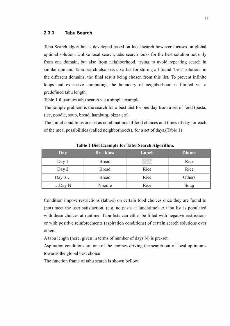
2.3.3 Tabu Search
Tabu Search algorithm is developed based on local search however focuses on global
optimal solution. Unlike local search, tabu search looks for the best solution not only
from one domain, but also from neighborhood, trying to avoid repeating search in
similar domain. Tabu search also sets up a list for storing all found ’best’ solutions in
the different domains, the final result being chosen from this list. To prevent infinite
loops and excessive computing, the boundary of neighborhood is limited via a
predefined tabu length.
Table 1 illustrates tabu search via a simple example.
The sample problem is the search for a best diet for one day from a set of food (pasta,
rice, noodle, soup, bread, hamburg, pizza,etc).
The initial conditions are set as combinations of food choices and times of day for each
of the meal possibilities (called neighborhoods), for a set of days.(Table 1)
Table 1 Diet Example for Tabu Search Algorithm.
Day Breakfast Lunch Dinner
Day 1 Bread Pasta Rice
Day 2 Bread Rice Rice
Day 3… Bread Rice Others
…Day N Noodle Rice Soup
Condition impose restrictions (tabu-s) on certain food choices once they are found to
(not) meet the user satisfaction. (e.g. no pasta at lunchtime). A tabu list is populated
with these choices at runtime. Tabu lists can either be filled with negative restrictions
or with positive reinforcements (aspiration conditions) of certain search solutions over
others.
A tabu length (here, given in terms of number of days N) is pre-set.
Aspiration conditions are one of the engines driving the search out of local optimums
towards the global best choice
The function frame of tabu search is shown bellow:
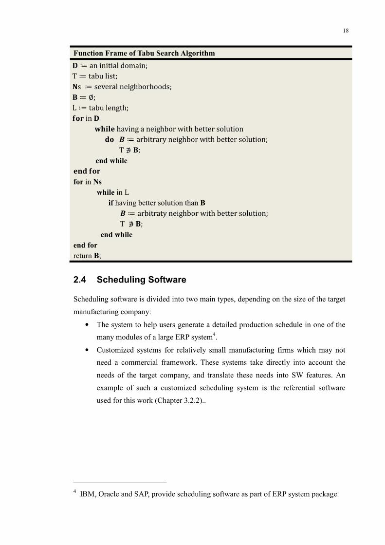
18
Function Frame of Tabu Search Algorithm
) ≔ an initial domain;
T ≔ tabu list;
,s ≔ several neighborhoods;
B ≔ ∅;
L ∶= tabu length;
��� in )
����� having a neighbor with better solution
$� / ≔ arbitrary neighbor with better solution;
T ∌ 1;
end while
�&$ ���
for in Ns
while in L
if having better solution than B
/ ≔ arbitraty neighbor with better solution;
T ∌ 1;
end while
end for
return B;
2.4 Scheduling Software
Scheduling software is divided into two main types, depending on the size of the target
manufacturing company:
• The system to help users generate a detailed production schedule in one of the
many modules of a large ERP system4.
• Customized systems for relatively small manufacturing firms which may not
need a commercial framework. These systems take directly into account the
needs of the target company, and translate these needs into SW features. An
example of such a customized scheduling system is the referential software
used for this work (Chapter 3.2.2)..
4 IBM, Oracle and SAP, provide scheduling software as part of ERP system package.

19
2.5 ISA 95 Standard
ISA 95 (ANSI/ISA–95.00.01–2000, 2000) is the international standard that integrates
enterprise and control systems. ISA 95 defines five levels in integration architecture
(Figure 9):
Figure 9: Function Classification. (ANSI/ISA–95.00.01–2000, 2000)
Business planning and logistic (the highest). This part mainly includes production
scheduling and operation management, at enterprise level.
Level 4 focuses on e.g. the collecting and maintaining materials, goods in process,
quality control and predictive maintenance planning. The basic production schedule
establishing is also included in Level 4. From the definition of Level 4, it is a similar
structure of ERP system and contains more parameters and other functions.
Level 3 is a transition part from enterprise management to manufacturing system. If
Level 4 is focused on global collecting and general function of enterprise, Level 3
focuses on Manufacturing Execution System (MES) level including the details of
production schedule and optimization, data collection and analysis for MES level, area
production reports etc.
20
3. Technical Approach
3.1 Standard
The main modules interacting with the Production Scheduling module implemented in
this thesis include (Figure 10):
� Order Processing,
� Material and Energy Control,
� Production Inventory Control and
� Production Control Systems.
The Production Scheduling module declares its availability for processing scheduling
requests to the Order Processing module, and its resource requirements to Production
Inventory Control. (The scheduling algorithm has to account for inventory limitations.)
This thesis implementation focuses on one-way Production Scheduling � Production
Control communication of information. The implementation of Production Control
� Production Scheduling information flow is out of the scope of this work..
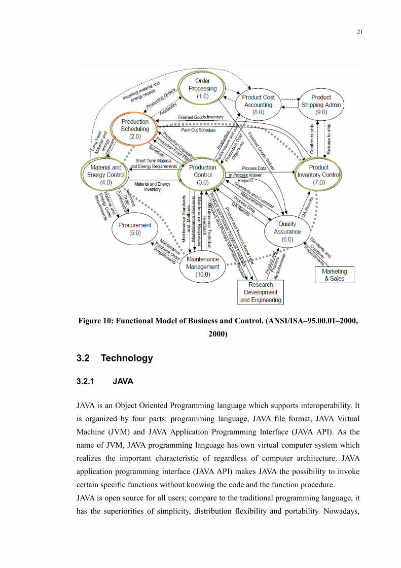
21
Figure 10: Functional Model of Business and Control. (ANSI/ISA–95.00.01–2000,
2000)
3.2 Technology
3.2.1 JAVA
JAVA is an Object Oriented Programming language which supports interoperability. It
is organized by four parts: programming language, JAVA file format, JAVA Virtual
Machine (JVM) and JAVA Application Programming Interface (JAVA API). As the
name of JVM, JAVA programming language has own virtual computer system which
realizes the important characteristic of regardless of computer architecture. JAVA
application programming interface (JAVA API) makes JAVA the possibility to invoke
certain specific functions without knowing the code and the function procedure.
JAVA is open source for all users; compare to the traditional programming language, it
has the superiorities of simplicity, distribution flexibility and portability. Nowadays,
22
JAVA has already become the most popular open-source programming language used
by most of the company for computer and mobile software development.
3.2.2 Referential Software
Drools (Drools, 2013) platform is developed by Redhat Company. It is a business rule
management system aiming to provide a knowledge base and interact with the
inference engine via a simple application programming interface (API). Drools is a
forward chaining production rules system. A rule engine based on rete algorithm stands
at the core of Drools. The Rule Engine (RE) sets the rules and finds the best match data
for setting targets. Rete Algorithm (RA) was designed by Dr Charles L. Forgy, to find a
matched pattern through building a network5, and relies on four main concepts: fact,
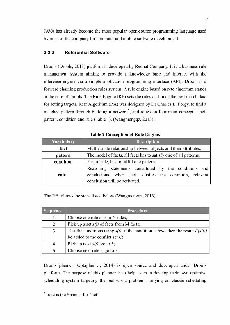
pattern, condition and rule (Table 1). (Wangmengqz, 2013) .
Table 2 Conception of Rule Engine.
Vocabulary Description
fact Multivariate relationship between objects and their attributes.
pattern The model of facts, all facts has to satisfy one of all patterns.
condition Part of rule, has to fulfill one pattern.
rule
Reasoning statements constituted by the conditions and
conclusions, when fact satisfies the condition, relevant
conclusion will be activated.
The RE follows the steps listed below (Wangmengqz, 2013):
Sequence Procedure
1 Choose one rule r from N rules;
2 Pick up a set s(f) of facts from M facts;
3 Test the conditions using s(f), if the condition is true, then the result R(s(f))
be added to the conflict set C;
4 Pick up next s(f), go to 3;
5 Choose next rule r, go to 2.
Drools planner (Optaplanner, 2014) is open source and developed under Drools
platform. The purpose of this planner is to help users to develop their own optimize
scheduling system targeting the real-world problems, relying on classic scheduling
5 rete is the Spanish for “net”
23
solutions (including e.g. the sales man problem, nQueens problem, vehicle route
problem etc.).
The solver implementations for these classic problems are provided by the Planner; the
user can directly change parameters and chain connections of problem entities
according to the analyzed problems and use the solver for getting solutions in order to
optimize production.
The system consists of three parts: the Model, the Rules and the Solver. The Model is
an information system that contains all data and parameters of the objective. The rules
are constraints to control the optimization of the final result, and are of two types: hard
and soft (the latter allow conditions imposed on the system to make it possible to
compute the schedule). According to the model and rules, the system will give score to
all generated solutions, with time limitation the best solution will printout.
Table 2 illustrates an example of storage of three types of products. There are three
types of products: A, B, and C, and the capacity of one storage is seven products in
total. An order is showing as below:
Table 3 Order list.
Type Pack One 6 Pack Two Pack Three
A 3 2 1
B 5 6 3
C 7 4 4
Problem goals: to fill storage space, and use the least amount of storages.
Fixed constraint: one pack of the products in each type cannot be separated in different
storages.
According to the problem, the model is easy to build:
� Objective:
Product type three: A, B, and C
Storage Capacity: 7
� Constraints of the problem:
Hard constraint: the pack of different type cannot be separated
Soft constraint: combination of the types should close to 7 in one storage.
6 Package of one type products, cannot be separate when storing. Numbers refer to the
current number of items in one package waiting for packing.
24
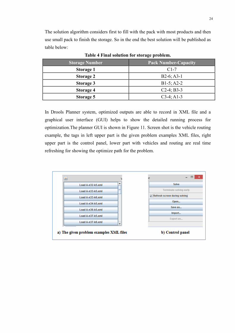
The solution algorithm considers first to fill with the pack with most products and then
use small pack to finish the storage. So in the end the best solution will be published as
table below:
Table 4 Final solution for storage problem.
Storage Number Pack Number-Capacity
Storage 1 C1-7
Storage 2 B2-6; A3-1
Storage 3 B1-5; A2-2
Storage 4 C2-4; B3-3
Storage 5 C3-4; A1-3
In Drools Planner system, optimized outputs are able to record in XML file and a
graphical user interface (GUI) helps to show the detailed running process for
optimization.The planner GUI is shown in Figure 11. Screen shot is the vehicle routing
example, the tags in left upper part is the given problem examples XML files, right
upper part is the control panel, lower part with vehicles and routing are real time
refreshing for showing the optimize path for the problem.
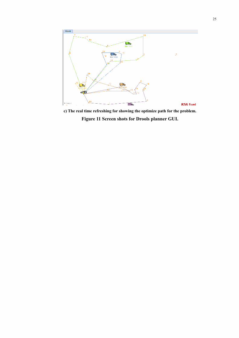
25
c) The real time refreshing for showing the optimize path for the problem.
Figure 11 Screen shots for Drools planner GUI.
26
4. Implementation
4.1 Test bed description
The test line is a full automation assembly line. There are twelve work cells working
for assembling mobile phones. Robots are adapted for using pens to draw pictures
instead of real assembly work.
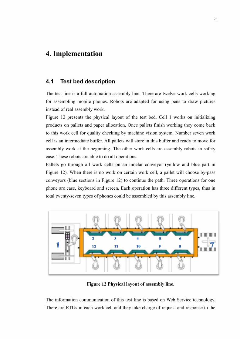
Figure 12 presents the physical layout of the test bed. Cell 1 works on initializing
products on pallets and paper allocation. Once pallets finish working they come back
to this work cell for quality checking by machine vision system. Number seven work
cell is an intermediate buffer. All pallets will store in this buffer and ready to move for
assembly work at the beginning. The other work cells are assembly robots in safety
case. These robots are able to do all operations.
Pallets go through all work cells on an innelar conveyor (yellow and blue part in
Figure 12). When there is no work on certain work cell, a pallet will choose by-pass
conveyors (blue sections in Figure 12) to continue the path. Three operations for one
phone are case, keyboard and screen. Each operation has three different types, thus in
total twenty-seven types of phones could be assembled by this assembly line.
Figure 12 Physical layout of assembly line.
The information communication of this test line is based on Web Service technology.
There are RTUs in each work cell and they take charge of request and response to the

27
other components, at the same time, they also send statues and data of the system to
other users from wireless network or internet so that those who are interested in this
system could also monitoring and control in a long distance. Figure 13 is the diagram
for the communication between devices of this assembly line.
Figure 13 System Communication Architecture. (Moctezuma, Jokinen, Postelnicu,
& Lastra, 2012)
4.2 Software implementation
The control system of the test assembly line originally played at the same time both
routing decision making role and low level (device-level) control.
The advantages of the proposed scheduling system include:
• Support to diagnose faults in the overall system without the need to interrupt
the functioning of unaffected equipment parts while conducting the
investigations.
• Interoperability support (XML outputs facilitate integration to most industry
system platforms).
28
4.2.1 Implementation Architecture
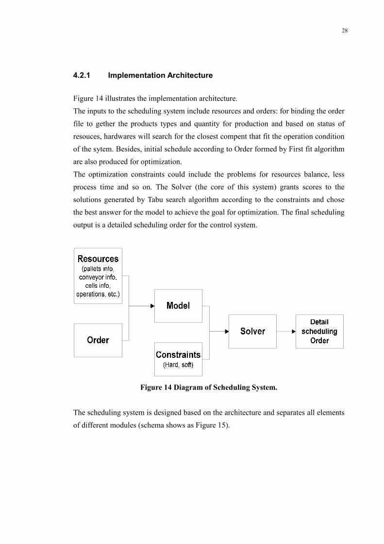
Figure 14 illustrates the implementation architecture.
The inputs to the scheduling system include resources and orders: for binding the order
file to gether the products types and quantity for production and based on status of
resouces, hardwares will search for the closest compent that fit the operation condition
of the sytem. Besides, initial schedule according to Order formed by First fit algorithm
are also produced for optimization.
The optimization constraints could include the problems for resources balance, less
process time and so on. The Solver (the core of this system) grants scores to the
solutions generated by Tabu search algorithm according to the constraints and chose
the best answer for the model to achieve the goal for optimization. The final scheduling
output is a detailed scheduling order for the control system.
Figure 14 Diagram of Scheduling System.
The scheduling system is designed based on the architecture and separates all elements
of different modules (schema shows as Figure 15).
29
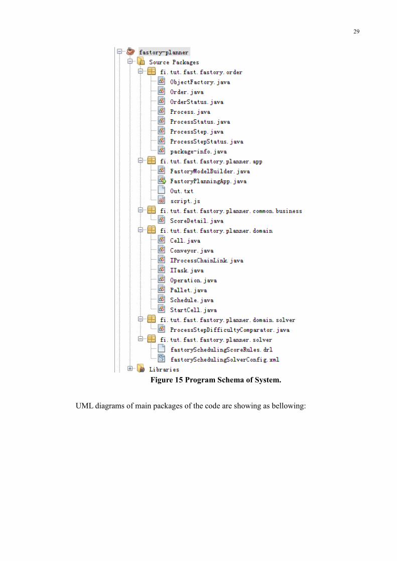
Figure 15 Program Schema of System.
UML diagrams of main packages of the code are showing as bellowing:
30
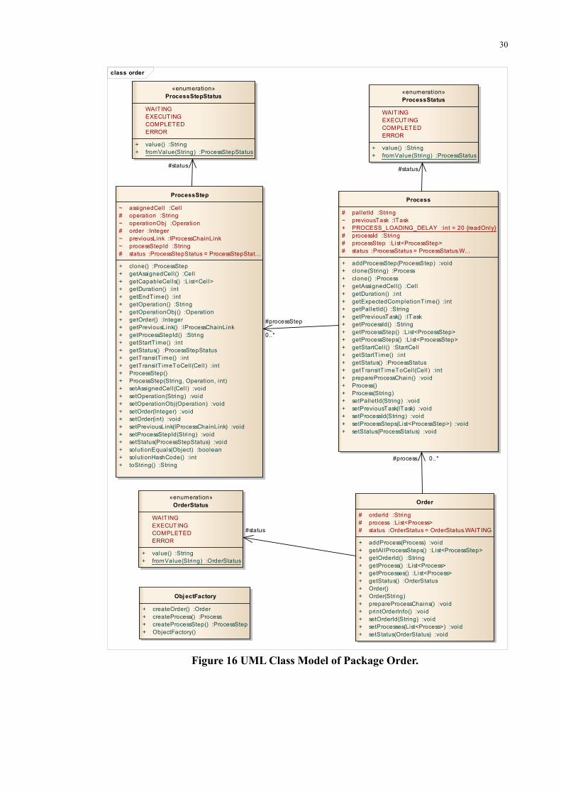
Figure 16 UML Class Model of Package Order.
class order
Obj ectFactory
+ createOrder() :Order
+ createProcess() :Process
+ createProcessStep() :ProcessStep
+ ObjectFactory()
Order
# orderId :String
# process :List<Process>
# status :OrderStatus = OrderStatus.WAITING
+ addProcess(Process) :void
+ getAllProcessSteps() :List<ProcessStep>
+ getOrderId() :String
+ getProcess() :List<Process>
+ getProcesses() :List<Process>
+ getStatus() :OrderStatus
+ Order()
+ Order(String)
+ prepareProcessChains() :void
+ printOrderInfo() :void
+ setOrderId(String) :void
+ setProcesses(List<Process>) :void
+ setStatus(OrderStatus) :void
«enumeration»
OrderStatus
WAITING
EXECUTING
COMPLETED
ERROR
+ value() :String
+ fromValue(String) :OrderStatus
Process
# palletId :String
~ previousTask :ITask
+ PROCESS_LOADING_DELAY :int = 20 {readOnly}
# processId :String
# processStep :List<ProcessStep>
# status :ProcessStatus = ProcessStatus.W...
+ addProcessStep(ProcessStep) :void
+ clone(String) :Process
+ clone() :Process
+ getAssignedCell() :Cell
+ getDuration() :int
+ getExpectedCompletionTime() :int
+ getPalletId() :String
+ getPreviousTask() :ITask
+ getProcessId() :String
+ getProcessStep() :List<ProcessStep>
+ getProcessSteps() :List<ProcessStep>
+ getStartCell() :StartCell
+ getStartTime() :int
+ getStatus() :ProcessStatus
+ getTransitTimeToCell(Cell) :int
+ prepareProcessChain() :void
+ Process()
+ Process(String)
+ setPalletId(String) :void
+ setPreviousTask(ITask) :void
+ setProcessId(String) :void
+ setProcessSteps(List<ProcessStep>) :void
+ setStatus(ProcessStatus) :void
«enumeration»
ProcessStatus
WAITING
EXECUTING
COMPLETED
ERROR
+ value() :String
+ fromValue(String) :ProcessStatus
ProcessStep
~ assignedCell :Cell
# operation :String
~ operationObj :Operation
# order :Integer
~ previousLink :IProcessChainLink
~ processStepId :String
# status :ProcessStepStatus = ProcessStepStat...
+ clone() :ProcessStep
+ getAssignedCell() :Cell
+ getCapableCells() :List<Cell>
+ getDuration() :int
+ getEndTime() :int
+ getOperation() :String
+ getOperationObj() :Operation
+ getOrder() :Integer
+ getPreviousLink() :IProcessChainLink
+ getProcessStepId() :String
+ getStartTime() :int
+ getStatus() :ProcessStepStatus
+ getTransitTime() :int
+ getTransitTimeToCell(Cell) :int
+ ProcessStep()
+ ProcessStep(String, Operation, int)
+ setAssignedCell(Cell) :void
+ setOperation(String) :void
+ setOperationObj(Operation) :void
+ setOrder(Integer) :void
+ setOrder(int) :void
+ setPreviousLink(IProcessChainLink) :void
+ setProcessStepId(String) :void
+ setStatus(ProcessStepStatus) :void
+ solutionEquals(Object) :boolean
+ solutionHashCode() :int
+ toString() :String
«enumeration»
ProcessStepStatus
WAITING
EXECUTING
COMPLETED
ERROR
+ value() :String
+ fromValue(String) :ProcessStepStatus
#status#status
#processStep
0..*
#status
#process 0..*
31
Figure 17 UML Class Model of Package APP.
Figure 18 UML Class Model of Package Business.
class app
FastoryModelBuilder
~ cells :Map<String, Cell>
~ context :JAXBContext
~ conveyors :Map<String, Conveyor>
~ marshaller :Marshaller
~ operations :Map<String, Operation>
~ order :Order
~ pallets :Map<String, Pallet>
~ solver :Solver
+ SOLVER_CONFIG :String = "/fi /tut/fast/f... {readOnly}
~ unmarshaller :Unmarshaller
+ buildModel() :void
+ buildNewPlanningProblem(Order) :Schedule
+ buildNewPlanningProblem() :Schedule
+ buildNewPlanningProblem(int) :Schedule
+ builPlanningProblemFromOrderXml(String) :Schedule
+ FastoryModelBuilder()
+ fi l terDescription(String) :List<Operation>
+ generateRandomOrder(String, int, int[]) :Order
+ generateRandomOrder(String, int) :Order
+ getAttachedCell(Conveyor) :Cell
+ initial ize(Schedule) :void
+ loadOrderFromXml(String) :Order
+ printSystemOverview() :void
+ random(int, int) :int
+ random(int, int, int) :int[]
+ randomOp(List<Operation>) :Operation
+ readOp(List<Operation>, int) :Operation
+ saveOrder(Order) :void
+ saveOrder() :void
FastoryPlanningApp
~ guiScoreDirector :ScoreDirector
~ optimal :Solution
~ solver :Solver
+ getScoreDetailList() :List<ScoreDetail>
+ init() :void
+ initSolver() :Solver
+ main(String[]) :void
+ registerForBestSolutionChanges() :void
+ reportNewBestSolution(Solution) :void
+ solve(Solution) :void
class business
Comparable
ScoreDetail
- constraintOccurrenceSet :Set<ConstraintOccurrence> = new HashSet<Con...
- constraintType :ConstraintType
- ruleId :String
- scoreTotal :double = 0.0
+ addConstraintOccurrence(ConstraintOccurrence) :void
+ bui ldConstraintOccurrenceListText() :String
+ compareTo(ScoreDetai l) :int
+ equals(Object) :boolean
+ getConstraintOccurrenceSet() :Set<ConstraintOccurrence>
+ getConstraintType() :ConstraintType
+ getOccurrenceSize() :int
+ getRuleId() :String
+ getScoreTotal() :double
+ hashCode() :int
+ ScoreDetail(String, ConstraintType)
+ toString() :String
32
Figure 19 UML Class Model of Package Domain.
Table 6 lists the packages and shortly describes their purpose..
class domain
Cell
~ capabi l ities :List<Operation> = new ArrayList<O...
- cellId :String
~ conveyor :Conveyor
~ status :Cel lStatus = CellStatus.WAITING
+ addCapabi l ity(Operation) :void
+ Cell()
+ Cell(String, Conveyor)
+ getCapabil ities() :List<Operation>
+ getCel lId() :String
+ getConveyor() :Conveyor
+ getStatus() :CellStatus
+ getT imeFromCell (Cell ) :int
+ hasCapabil ity(Operation) :boolean
+ setCapabil i ties(List<Operation>) :void
+ setCell Id(String) :void
+ setConveyor(Conveyor) :void
+ setStatus(Cel lStatus) :void
+ toString() :String
«enumerati ...
Cell::CellStatus
WAITING
WORKING
READY
OFFLINE
Conv eyor
~ bypass :boolean
~ id :String
~ nextConveyor :Conveyor
~ transitT ime :int = 5
+ Conveyor(String)
+ equals(Conveyor) :boolean
+ getId() :String
+ getNextConveyor() :Conveyor
+ getTotalTransitT imeToConveyor(Conveyor) :int
+ getTransi tT ime() :int
+ hasBypass() :boolean
+ setBypass(boolean) :void
+ setNextConveyor(Conveyor) :void
+ setTransi tT ime(int) :void
+ toString() :String
«interface»
IProcessChainLink
+ getAssignedCell () :Cell
+ getDuration() :int
+ getStartTime() :int
+ getTransitTimeToCell(Cell) :int
«interface»
ITask
+ getStartT ime() :int
Operation
~ capableCells :List<Cell> = new ArrayList<C...
~ description :String
~ duration :int
~ id :String
+ addCapableCell(Cell) :void
+ getCapableCel ls() :List<Cell>
+ getDescription() :String
+ getDuration() :int
+ getId() :String
+ Operation(String, String, int)
+ setCapableCells(Collection<Cell>) :void
+ toString() :String
Pallet
~ cel l :Cell
~ id :String
~ status :PalletStatus
+ getCell() :Cell
+ Pal let(String)
+ setStartingCel l(Cel l) :void
«property get»
+ getid() :String
«enumeration»
Pallet::PalletStatus
UNKNOWN
INTRANSIT
READY
INPROCESSING
OFFLINE
Solution
Schedule
- cellList :List<Cell>
- name :String
- order :Order
- processStepList :List<ProcessStep>
- score :HardAndSoftScore
+ cloneSolution() :Schedule
+ equals(Object) :boolean
+ getCel lList() :List<Cell>
+ getName() :String
+ getOrder() :Order
+ getProblemFacts() :Collection<? extends Object>
+ getProcessList() :List<Process>
+ getProcessStepList() :List<ProcessStep>
+ getScore() :HardAndSoftScore
+ getStartCel ls() :List<StartCel l>
+ hashCode() :int
+ printStats() :void
+ setCellList(List<Cell>) :void
+ setName(String) :void
+ setOrder(Order) :void
+ setScore(HardAndSoftScore) :void
StartCell
+ getStartT ime() :int
+ StartCel l()
+ StartCel l(String, Conveyor)
-cellList 0..*
~status
~cell
~capableCel ls 0..*
~status
~conveyor
~capabil i ties 0..*
33
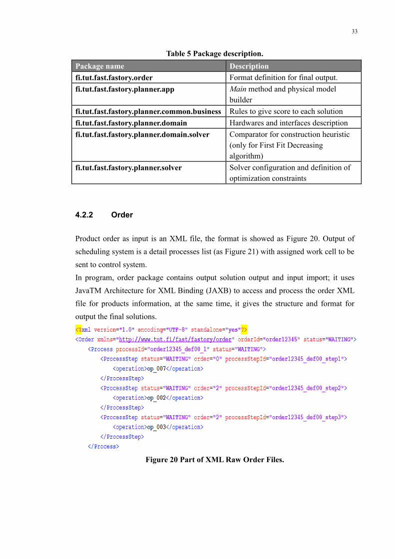
Table 5 Package description.
Package name Description
fi.tut.fast.fastory.order Format definition for final output.
fi.tut.fast.fastory.planner.app Main method and physical model
builder
fi.tut.fast.fastory.planner.common.business Rules to give score to each solution
fi.tut.fast.fastory.planner.domain Hardwares and interfaces description
fi.tut.fast.fastory.planner.domain.solver Comparator for construction heuristic
(only for First Fit Decreasing
algorithm)
fi.tut.fast.fastory.planner.solver Solver configuration and definition of
optimization constraints
4.2.2 Order
Product order as input is an XML file, the format is showed as Figure 20. Output of
scheduling system is a detail processes list (as Figure 21) with assigned work cell to be
sent to control system.
In program, order package contains output solution output and input import; it uses
JavaTM Architecture for XML Binding (JAXB) to access and process the order XML
file for products information, at the same time, it gives the structure and format for
output the final solutions.
Figure 20 Part of XML Raw Order Files.
34
Figure 21 Output Detail Process Order.
Order package provides schema for the input order parameters:
� ObjectFactory: create order schema.
� Order: provides schema of complex type for element of order in XML file which
contains all information about order ID and the status of order. It defines the final
printed output value according to product order as well.
� Process: schema for the element of process in XML file. Process has processId,
status, palletId and ProcessStep. Every process refers to one product therefore
production information such as process duration, start time, assigned cell and
transit time from cells are also provide in this file.
� Processstep: schema for ProcessStep, includes operationObj, status and order.
Method for operation process time calculation is also included.
� OrderStatus, ProcessStatus, ProcessStepStatus: four status in total, they are:
“EXECUTING”: object is under processing.
“WAITING”: object gets ready for process
“COMPLETED”: object finished processing, production are able to do next step.
“ERROR”: object is unable to be processed; some problems could be machine
breakdown or pallet traffic crash.
4.2.3 Application
Two parts in this package: module builder and application running (main method).
35
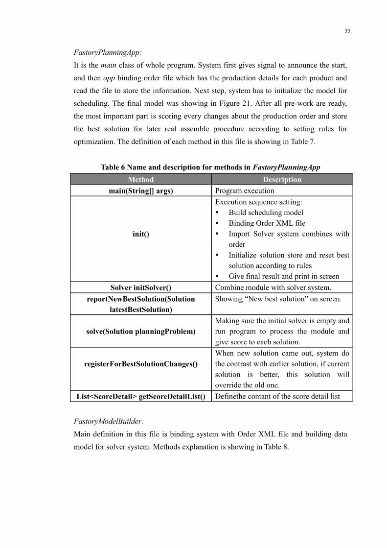
FastoryPlanningApp:
It is the main class of whole program. System first gives signal to announce the start,
and then app binding order file which has the production details for each product and
read the file to store the information. Next step, system has to initialize the model for
scheduling. The final model was showing in Figure 21. After all pre-work are ready,
the most important part is scoring every changes about the production order and store
the best solution for later real assemble procedure according to setting rules for
optimization. The definition of each method in this file is showing in Table 7.
Table 6 Name and description for methods in FastoryPlanningApp
Method Description
main(String[] args) Program execution
init()
Execution sequence setting:
� Build scheduling model
� Binding Order XML file
� Import Solver system combines with
order
� Initialize solution store and reset best
solution according to rules
� Give final result and print in screen
Solver initSolver() Combine module with solver system.
reportNewBestSolution(Solution
latestBestSolution)
Showing “New best solution” on screen.
solve(Solution planningProblem)
Making sure the initial solver is empty and
run program to process the module and
give score to each solution.
registerForBestSolutionChanges()
When new solution came out, system do
the contrast with earlier solution, if current
solution is better, this solution will
override the old one.
List<ScoreDetail> getScoreDetailList() Definethe contant of the score detail list
FastoryModelBuilder:
Main definition in this file is binding system with Order XML file and building data
model for solver system. Methods explanation is showing in Table 8.

36
Table 7 Main methods names and description for FastoryModelBuilder
Method Description
FastoryModelBuilder() Build architecture for Order XML
binding, create marshaled and
unmarshaller objects.
Schedule buildNewPlanningProblem(Order
order)
Get into schedule file and the database
is using Order data
Schedule buildNewPlanningProblem(int
productCount)
Initial the count of product of order
Schedule
builPlanningProblemFromOrderXml(String
filename)
Get file name of order XML file.
buildModel() Building model for scheduling
system.
� Create conveyor loop, each
conveyor has corresponding cell
and it is chain structure.
� List cells from number one to
twelve
� Define pallet number is 20, all
pallet starts from cell 7 which is
buffer station.
� Operation definition. Three
actions are doing as operations;
they are keyboard, screen and
case. Each action has three
different types spending another
time. Model defines three actions
are done in separated cells, cell
one is installing station, cell seven
is buffer, rest cells are able to do
any actions. Case action operates
on first four cells, the rest
operation cells are chosen to do
keyboard and screen actions.
printSystemOverview() Declare the final system output
overview on Output window.
getAttachedCell(Conveyor c) Attach cell to corresponding
conveyor.
Operation readOp(List<Operation> ops, int
t)
Get operation information.
random(int min, int max) Mathematical method. Choose
37
random number from given numbers.
List<Operation> filterDescription(String
filter)
Filter operation with certain filter
characters.
random(int min, int max, int n) Random choose n numbers from min
to max.
initialize(Schedule s) As method name says initialize
schedule.
Order loadOrderFromXml(String filename) Load an Order from XML file.
Order generateRandomOrder(String
orderId, int nDefs, int[] quantities)
Put Order in JAVA system and
generate initial order for scheduling.
4.2.4 Domain
The physical components of the assembly line are pallets, conveyors, work cells,
dynamic objects of assembly production are operations and schedule for production.
Domain package give definition of all parameters of these objectives.
� Cell: definition includes cell ID, status, and relevant conveyors.
� Conveyor: basic information contents ID, pallet transit time, and the connection
with downstream conveyor.
� Pallet: pallet ID, status of the pallet and the first operation cell where the process
starts.
� StartCell: it is the extension for cell to define the lead cell for the pallet route and
calculate the process time.
� Schedule: scheduling procedures, the first thing is gathering all information for
scheduling system which includes order, cells, processes list and so on, the next is
using drools score system and override it at each time the score is better than
before. Finally schedule prints the best solution after optimization.
� ITask: interface, defined as getStartTime.
� IProcessChainLink: interface, contents several method signatures and constant
declarations.
38
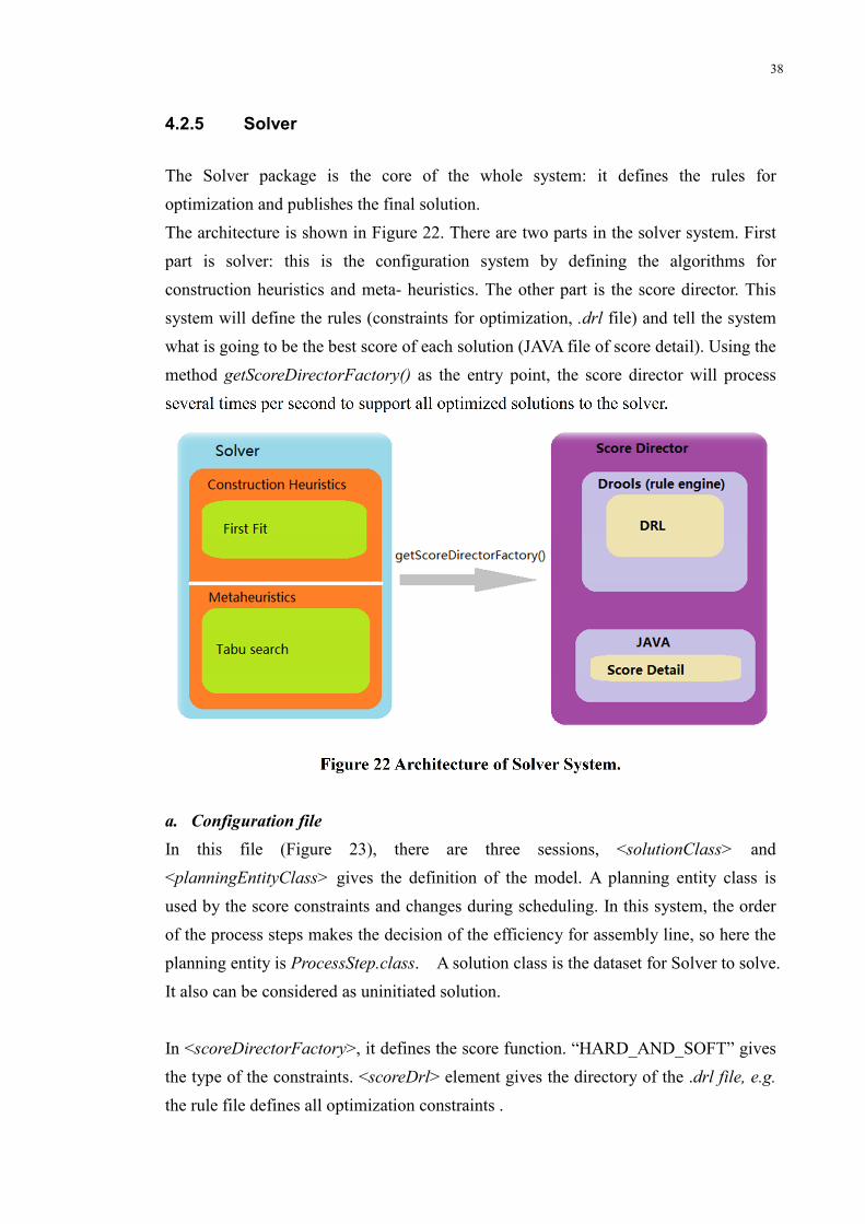
4.2.5 Solver
The Solver package is the core of the whole system: it defines the rules for
optimization and publishes the final solution.
The architecture is shown in Figure 22. There are two parts in the solver system. First
part is solver: this is the configuration system by defining the algorithms for
construction heuristics and meta- heuristics. The other part is the score director. This
system will define the rules (constraints for optimization, .drl file) and tell the system
what is going to be the best score of each solution (JAVA file of score detail). Using the
method getScoreDirectorFactory() as the entry point, the score director will process
several times per second to support all optimized solutions to the solver.
Figure 22 Architecture of Solver System.
a. Configuration file
In this file (Figure 23), there are three sessions, <solutionClass> and
<planningEntityClass> gives the definition of the model. A planning entity class is
used by the score constraints and changes during scheduling. In this system, the order
of the process steps makes the decision of the efficiency for assembly line, so here the
planning entity is ProcessStep.class. A solution class is the dataset for Solver to solve.
It also can be considered as uninitiated solution.
In <scoreDirectorFactory>, it defines the score function. “HARD_AND_SOFT” gives
the type of the constraints. <scoreDrl> element gives the directory of the .drl file, e.g.
the rule file defines all optimization constraints .
39
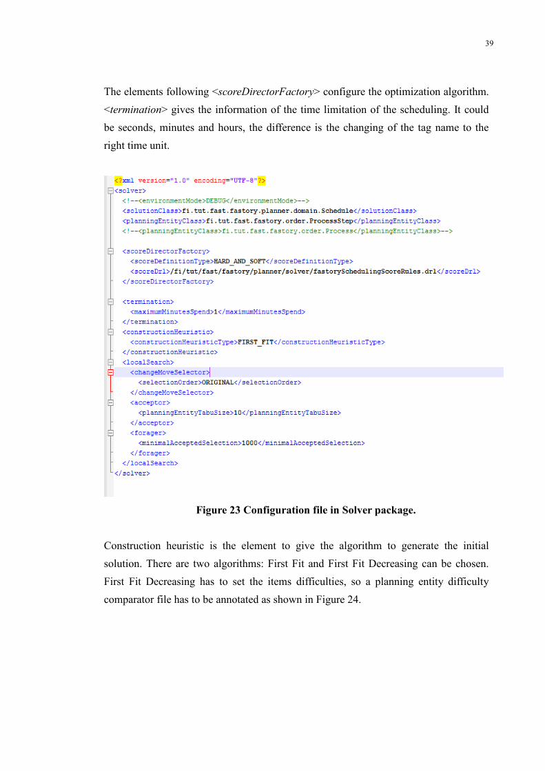
The elements following <scoreDirectorFactory> configure the optimization algorithm.
<termination> gives the information of the time limitation of the scheduling. It could
be seconds, minutes and hours, the difference is the changing of the tag name to the
right time unit.
Figure 23 Configuration file in Solver package.
Construction heuristic is the element to give the algorithm to generate the initial
solution. There are two algorithms: First Fit and First Fit Decreasing can be chosen.
First Fit Decreasing has to set the items difficulties, so a planning entity difficulty
comparator file has to be annotated as shown in Figure 24.
40
Figure 24 Planning entity difficulty comparison.
The changes from one solution to another solution is called “move”, a MoveSelector's
main function is to create Iterator<Move> when needed. There are three methods to
choose the “move”, original, random and shuffled.
Original: the selector will follow the default order of the moves. All moves will be
chosen only once.
Random: random choose the moves, one move may be chosen twice or more.
Shuffled: shuffled random choose the moves, each move will be done only once.
<acceptor> makes decision whether the moves are accepted or not. The tube size for
planning entity has to do several tests to look for the arrangement. Number given in the
example is random.
<forager> helps the system to pick up the nest step from all gathered moves, the
default rule is choose the move with higher score, when several moves has same score,
forager will choose a random one from them. The sub element decides the number
limitation of accepted selection; it would be the more the better.
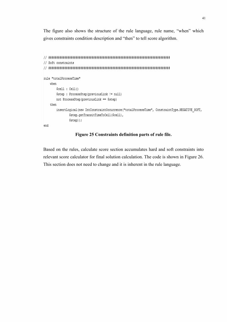
b. Rule file
Rule (.drl) file full name is called drools rules language. Users could change
constraints to meet the demand of the optimization.
In rule file, the language is call rule language. Figure 25 indicates how to define the
rules in .drl file. It could be positive and negative constraints, positive is the conditions
users try to do the maximum and negative is the ones users try to do the minimum.
According to the real scheduling case, we choose negative constraints only. The
definitions of the constraint are of two types:
Negative hard constraints: constrains that cannot be broken when the system executes.
Negative soft constraints: if this condition can be avoided, the system will be
optimized.
41
The figure also shows the structure of the rule language, rule name, “when” which
gives constraints condition description and “then” to tell score algorithm.
Figure 25 Constraints definition parts of rule file.
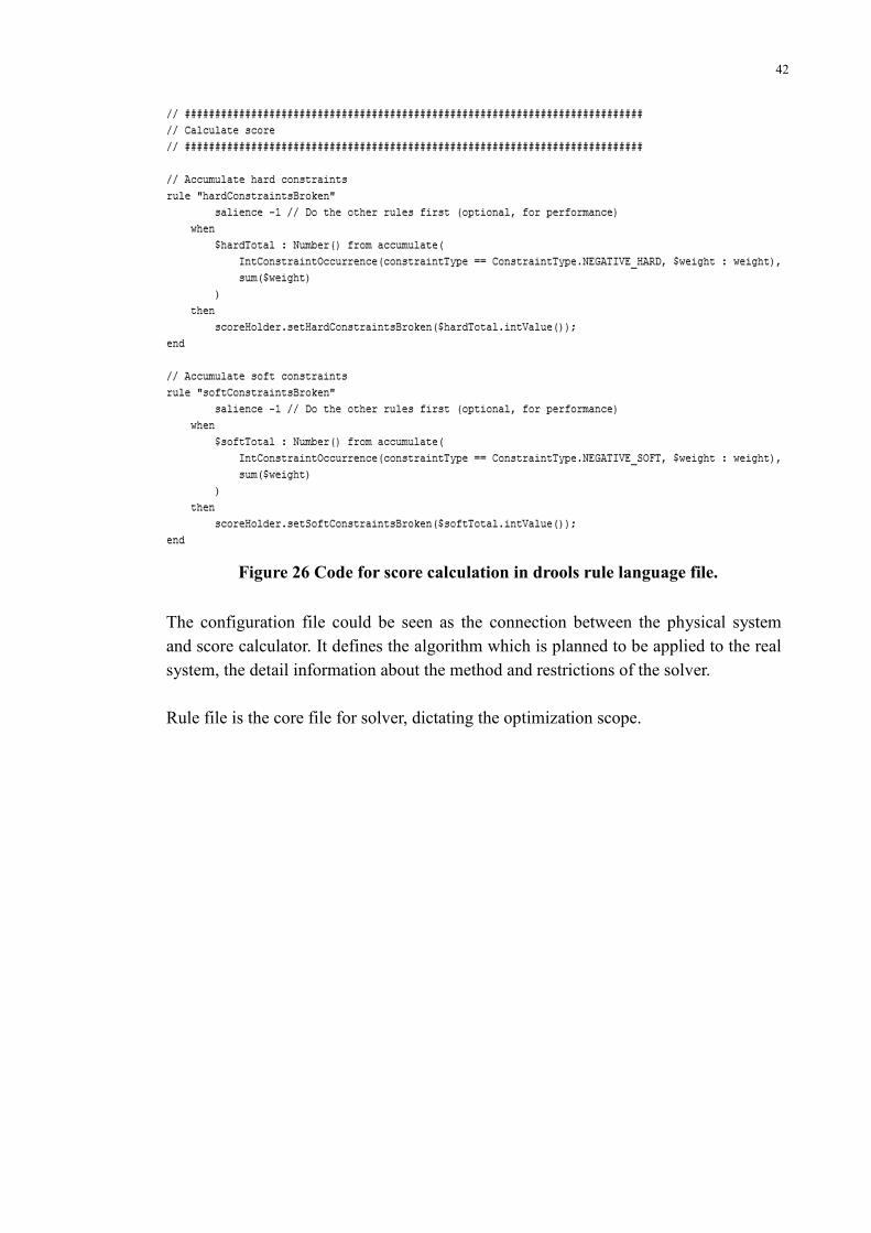
Based on the rules, calculate score section accumulates hard and soft constraints into
relevant score calculator for final solution calculation. The code is shown in Figure 26.
This section does not need to change and it is inherent in the rule language.
42
Figure 26 Code for score calculation in drools rule language file.
The configuration file could be seen as the connection between the physical system
and score calculator. It defines the algorithm which is planned to be applied to the real
system, the detail information about the method and restrictions of the solver.
Rule file is the core file for solver, dictating the optimization scope.
43
5. Results and Discussion
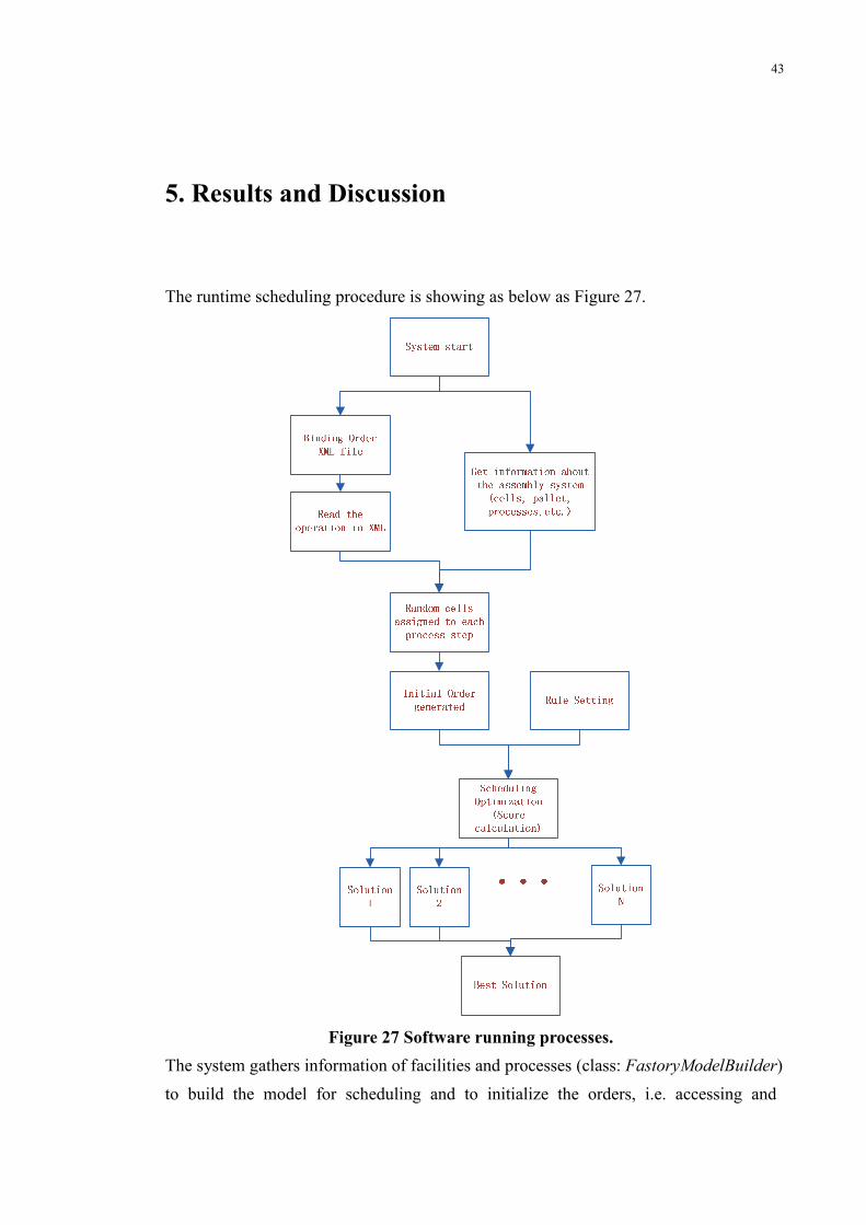
The runtime scheduling procedure is showing as below as Figure 27.
Figure 27 Software running processes.
The system gathers information of facilities and processes (class: FastoryModelBuilder)
to build the model for scheduling and to initialize the orders, i.e. accessing and
44
processing order XML file (package: fi.tut.fast.fastory.order) and make the order as an
initial schedule list. The following step is according to the problem and planning
entities, solver gets ready to do the search for better solutions (class: ScoreDetail) and
print out the final result (class: Schedule).
5.1 Result Presentation
The initialization step can be modified based on the real situation; outputs will show all
data of the setting system, which including the quantity and identify numbers of cells,
conveyors, pallets and operations. Screenshots bellowing reveals the outputs for
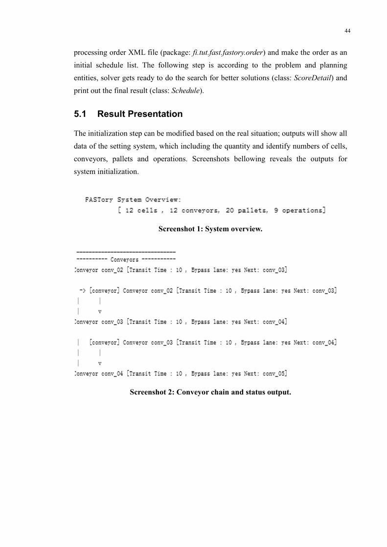
system initialization.
Screenshot 1: System overview.
Screenshot 2: Conveyor chain and status output.
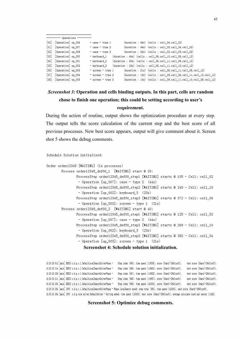
45
Screenshot 3: Operation and cells binding outputs. In this part, cells are random
chose to finish one operation; this could be setting according to user’s
requirement.
During the action of routine, output shows the optimization procedure at every step.
The output tells the score calculation of the current step and the best score of all
previous processes. New best score appears, output will give comment about it. Screen
shot 5 shows the debug comments.
Screenshot 4: Schedule solution initialization.
Screenshot 5: Optimize debug comments.

46
The final result (the best score) is setting time also printed in outputs. Cell usage is not
the working times of cells, but it is the working percentage of each cell.
Screenshot 6: Total time and usage of cells.
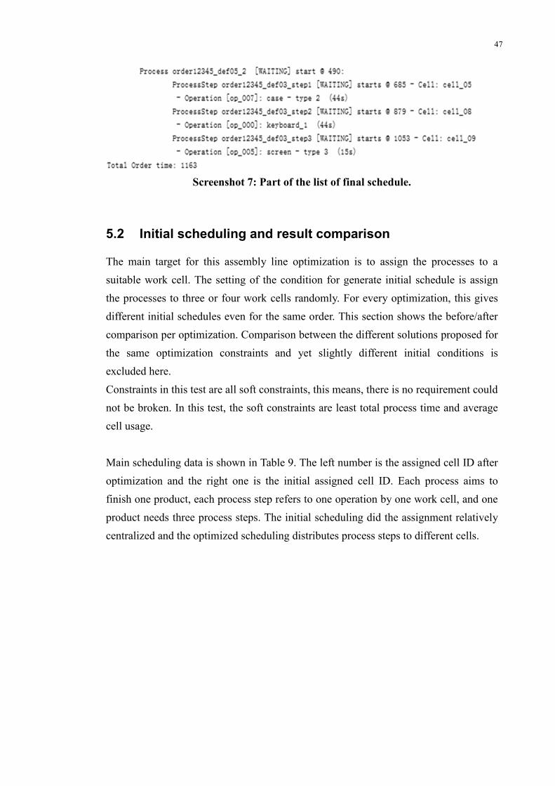
Final schedule will give detailed operation information to the downstream system. The
details include the start time of one order, the assigned cell of operation, information of
operations and order of all operations. The form of the list is:
Process “ID” “[state]” start @ “starting time”:
ProcessStep “ID” “[state]” start @ “starting time” – Cell: “AssignedCell”
- Operation [ID]: “OpertionType” (OperationSpendingTime)
Screenshot 7 indicates one part of the final optimized scheduling list.
47
Screenshot 7: Part of the list of final schedule.
5.2 Initial scheduling and result comparison
The main target for this assembly line optimization is to assign the processes to a
suitable work cell. The setting of the condition for generate initial schedule is assign
the processes to three or four work cells randomly. For every optimization, this gives
different initial schedules even for the same order. This section shows the before/after
comparison per optimization. Comparison between the different solutions proposed for
the same optimization constraints and yet slightly different initial conditions is
excluded here.
Constraints in this test are all soft constraints, this means, there is no requirement could
not be broken. In this test, the soft constraints are least total process time and average
cell usage.
Main scheduling data is shown in Table 9. The left number is the assigned cell ID after
optimization and the right one is the initial assigned cell ID. Each process aims to
finish one product, each process step refers to one operation by one work cell, and one
product needs three process steps. The initial scheduling did the assignment relatively
centralized and the optimized scheduling distributes process steps to different cells.
48
Table 8 Assigned cells comparison before and after optimization.
Process Step 1 Cell Id Process Step 2 Cell Id Process Step 3 Cell Id
Process 1 12 12 11 8 9 12
Process 2 9 3 8 11 6 6
Process 3 3 3 4 4 8 8
Process 4 3 3 5 5 3 6
Process 5 10 4 2 2 12 12
Process 6 6 12 2 2 12 12
Process 7 3 3 9 4 10 10
Process 8 10 10 4 4 4 4
Process 9 11 3 2 2 6 6
Process 10 11 11 4 2 10 10
Process 11 10 10 2 11 4 4
Process 12 4 4 6 6 9 6
Process 13 3 3 6 6 3 10
Process 14 3 3 2 2 9 5
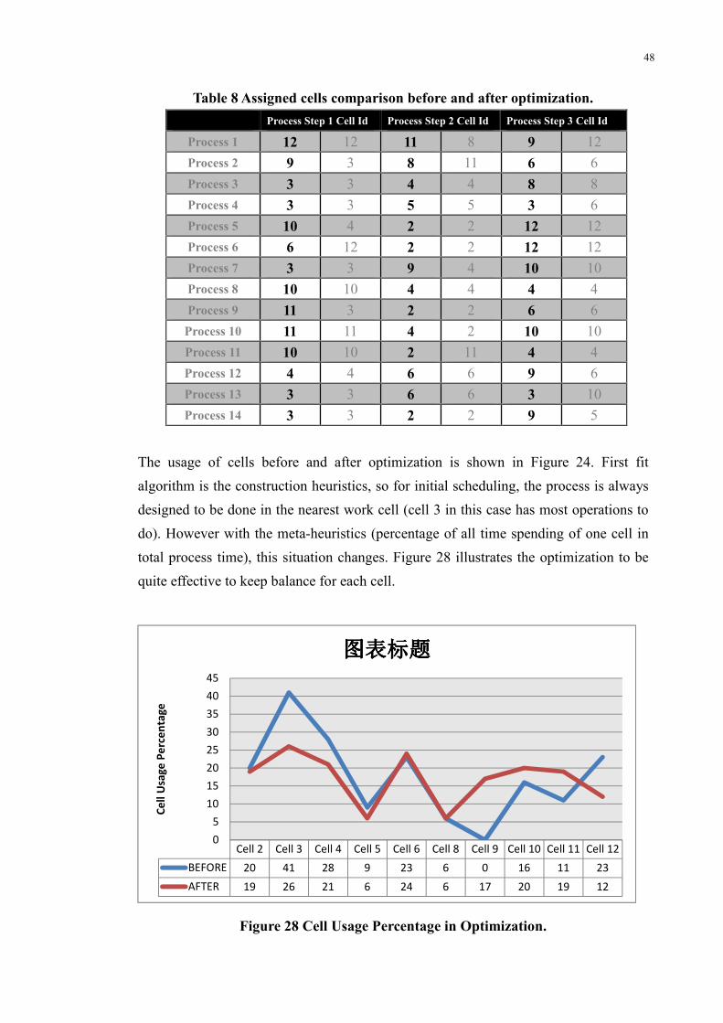
The usage of cells before and after optimization is shown in Figure 24. First fit
algorithm is the construction heuristics, so for initial scheduling, the process is always
designed to be done in the nearest work cell (cell 3 in this case has most operations to
do). However with the meta-heuristics (percentage of all time spending of one cell in
total process time), this situation changes. Figure 28 illustrates the optimization to be
quite effective to keep balance for each cell.
Figure 28 Cell Usage Percentage in Optimization.
Cell 2 Cell 3 Cell 4 Cell 5 Cell 6 Cell 8 Cell 9 Cell 10 Cell 11 Cell 12
BEFORE 20 41 28 9 23 6 0 16 11 23
AFTER 19 26 21 6 24 6 17 20 19 12
0
5
10
15
20
25
30
35
40
45
Ce
ll U
sag
e P
erc
en
tag
e
图表标题图表标题图表标题图表标题

49
Besides the balance for cell usage, the total process time is also under consideration,
(here increasing from 663 seconds to 683 seconds). This solution shows more
superiority in cell balance than total process time, and it also depends on the initial
schedule. Several scheduling trials will give different solutions for the same order;
each user could choose the best one based on different constraints weight, for example
the final optimal might focus on better resource balance than process time.
50
6. Conclusions
Today’s companies need manufacturing optimization, with specific focus on cost
reduction, energy savings and environmental issues. The master plan defined prior to
the commencing of the production must be coupled with scheduling algorithms that
would perform on manufacturing processes data acquired in RT.
The test bed for the scheduling system implemented in this thesis work is a dedicated
assembly line; the proposed system architecture could nevertheless be applied to any
type of production line.
The final optimization guidelines rely on constraints defined formally as rules.
Different initial conditions result in different optimization solutions proposed.
The system accomplishes scheduling optimization and gives satisfactory solutions for
optimization purpose.
Advantages of the proposed solutions include:
� Decoupling between facilities and the scheduling algorithm. The assembly line
could be built, in practice, by any component, the scheduling algorithm just pays
attention to several parameters from the large, i.e. identifying the planning entity
and constraints objects.
� Availability of problem-specific solutions. Local search has the defect that the
found solution might not prove suitable for all types of problems. In practice
though, clients may focus on different purposes for optimization, thus the local
search algorithm is able to find a ’best’ solution for certain specific problem. At
the same time, different initial schedules result in different solutions, each client
could choose the best one from these solutions.
� Flexibility on the solver side. Sample optimize planner provides several algorithms
for optimization, and the configuration file for solver offers all information about
optimization. Changing the parameters could also affect the optimized solutions.
51
References
ANSI/ISA–95.00.01–2000. (2000). In Enterprise-Control System Integration Part 1:
Models and Teminology (pp. 19-26). US.
Dósa, G., & Sgall, J. (1998). First Fit bin packing: A tight analysis. Leibniz
International Proceedings in Informatics (pp. 1-15). Dagstuhl Publishing.
Gantt, H. L. (1903). A graphical daily balance in manufacture. [ASME Transactions]
24, 1322-1336.
Herrmann, J. (2006). A history of production scheduling. In J. Herrmann (Ed.), (pp.
1-22) Springer US. doi:10.1007/0-387-33117-4_1
Hopp, W., & Spearman, M. (2004). Commissioned Paper To Pull or Not to Pull: What
Is the Question? Manufacturing & Service Operations Management, pp. 133-148.
Jammes, F. (n.d.). 05022-SODA-SODA_Innovation-report. ITEA.
L. Wylie, GartnerGroup. (April.1990). ERP: A Vision of the Next-Generation MRP II.
Marco, T., Colombo, A. W., & Karnouskos, S. (n.d.). SOCRADES ROADMAP.
SOCRADES.EU.
Pinedo, M. (2005). Introduction. Planning and scheduling in manufacturing and
services (pp. 8) Springer US.
Ryś, T., Stanek, R., & Ziembla, W. (1994). MIPS: A DSS for multiobjective interactive
project scheduling. European Journal of Operational Research, 79(2), 196-207.
doi:10.1016/0377-2217(94)90351-4
Tharumarajah, A., & Bemelman, R. (1997). Approaches and issues in scheduling a
distributed shop-floor environment. Computers in Industry, 34(1), 95–109.

52
Wu, C., Yushun, F., & Deyun, X. (2001). Chapter 15 computer integrated
manufacturing. In S. Gavriel (Ed.), Handbook of industrial engineering -
technology and operations management (3rd edition) (pp. 485) John Wiley & Sons
Inc.
53
Network References
Drools. [WWW]. [Accessed on 2013, May 16]. Available at:
https://www.jboss.org/drools/
Optaplanner. [WWW]. [Accessed on 2014, April 19]. Available at:
http://www.optaplanner.org/
Cuccok, p.. Elképesztő robottechnológia a Tesla gyárban. [WWW]. [Accessed on 2014,
April 20] Available at: http://www.pto.hu/post/1/12997
Frederick Winslow Taylor. [WWW]. [Accessed on 2014, April 19] Available at:
http://en.wikipedia.org/wiki/Frederick_Winslow_Taylor
Gongye Zidonghua Jishu He Fazhanshi. [WWW]. [Accessed on 2014, April 19]
Available at: http://wenku.baidu.com/view/67cc681c10a6f524ccbf852f.html
IMC-AESOP Project. [WWW]. [Accessed on 2014, May 10] Available at:
http://www.imc-aesop.eu
Infinion. Industrial Automation Efficient & Robust Semiconductor Solutions. [WWW].
[Accessed on 2014, April 3] Available at:
http://www.infineon.com/dgdl/Industrial_Automation_2013.pdf?folderId=db3a
30431689f4420116a096e1db033e&fileId=db3a30433cabdd35013cb48285386c
94
Integrate IT. [WWW]. [Accessed on 2013, May 15] Available at:
http://erp123.biz/erp-guide/erp-flowcharts-of-data/mrp-overview
Mahmoud, Q. H. (2005, April). Service-Oriented Architecture (SOA) and Web
Services: The Road to Enterprise Application Integration (EAI). [WWW].
[Accessed on 2013, May 15] Available at
http://www.oracle.com/technetwork/articles/javase/soa-142870.html
54
Material Requirements Planning . [WWW]. [Accessed on 2013, May 15] Available at:
http://en.wikipedia.org/wiki/Material_requirements_planning
MIE Scheduling Software 1. [WWW]. [Accessed on 2013, May 28] Available at:
http://www.softsia.com/MIE-Scheduling-Software-download-0z1d.htm
Sensen, N. Local Search Algorithms. [WWW]. [Accessed on 2013, May 27] Available
at
http://www2.cs.uni-paderborn.de/cs/ag-monien/PERSONAL/SENSEN/Schedul
ing/icpp/node5.html
Service-Oriented Architecture,SOA.[WWW]. [Accessed on 2014, April 19] Available
at:
http://wiki.mbalib.com/wiki/%E9%9D%A2%E5%90%91%E6%9C%8D%E5%
8A%A1%E6%9E%B6%E6%9E%84
Software as a service:ERP by the Hour and ERP Sytems: Do they Satisfy? (). [WWW].
[Accessed on 2013, May 15] Available at:
http://managementinfosystemsblogg.blogspot.fi/
Thorpe, G. (2013, May 16). Design For Purpose. [WWW]. [Accessed on 22.2.2006]
Available at: http://designforpurpose.blogspot.fi/
W3C.Web Services Glossary. [WWW]. [Accessed on 2013, May 27] Available at:
http://www.w3.org/TR/2004/NOTE-ws-gloss-20040211/#webservice
Wangmengqz. [WWW]. [Accessed on 2013, June 14] Available at:
http://bbs.csdn.net/topics/390113737