AN APPROXIMATION METHOD FOR EXACT CONTROLS OF …math.ucv.ro/~micu/auxiliare/work_ro/doc/papers/cmt.pdf · 2011-05-26 · AN APPROXIMATION METHOD FOR EXACT CONTROLS OF ... The algorithm

SIAM J. CONTROL OPTIM. c© XXXX Society for Industrial and Applied MathematicsVol. 0, No. 0, pp. 000–000

AN APPROXIMATION METHOD FOR EXACT CONTROLS OFVIBRATING SYSTEMS∗

NICOLAE CINDEA† , SORIN MICU‡ , AND MARIUS TUCSNAK†

Abstract. We propose a new method for the approximation of exact controls of a secondorder infinite dimensional system with bounded input operator. The algorithm combines Russell’s“stabilizability implies controllability” principle with the Galerkin method. The main new featureof this work consists of giving precise error estimates. In order to test the efficiency of the method,we consider two illustrative examples (with the finite element approximations of the wave and thebeam equations) and describe the corresponding simulations.

Key words. infinite dimensional systems, exact control, approximation, error estimate

AMS subject classifications. 35L10, 65M60, 93B05, 93B40, 93D15

DOI. 10.1137/09077641X

1. Introduction. The numerical study of the exact controls of infinite dimen-sional systems began in the 1990s with a series of papers by Glowinski and Lions(see [11, 12]) where algorithms for determining the minimal L2-norm exact controls(sometimes called HUM controls) are provided. Several abnormalities presented inthese papers motivated a large number of articles in which a great variety of numeri-cal methods are presented and analyzed (see, for instance, [33, 8] and the referencestherein). However, except for the recent work [9], where the approximation of theHUM controls for the one dimensional wave equation is considered, to our knowledge,there are no results on the rate of convergence of the approximative controls.

The aim of this work is to provide an efficient numerical method for computingexact controls for a class of infinite dimensional systems modeling elastic vibrations.Our main theoretical result gives the rate of convergence of our approximations to anexact control. Moreover, to illustrate the efficiency of this approach, we apply it toseveral systems governed by PDEs and describe the associated numerical simulations.Our methodology combines Russell’s “stabilizability implies controllability” principlewith error estimates for finite element-type approximations of the considered infinitedimensional systems. We focus on the case of bounded input operators which ex-cludes boundary control for systems governed by PDEs. However, the method can bepartially extended to the unbounded input operator case; see Remark 2.7.

In order to give the precise statement of our results we need some notation. LetH be a Hilbert space, and assume that A0 : D(A0) → H is a self-adjoint, strictlypositive operator with compact resolvent. Then, according to classical results, theoperator A0 is diagonalizable with an orthonormal basis (ϕk)k�1 of eigenvectors, andthe corresponding family of positive eigenvalues (λk)k�1 satisfies limk→∞ λk = ∞.

∗Received by the editors November 9, 2009; accepted for publication (in revised form) March4, 2011; published electronically DATE. This work was partially supported by the bilateral project19600SJ, grant 206/2009 of ANCS (Romania).

http://www.siam.org/journals/sicon/x-x/77641.html†Institut Elie Cartan, Nancy Universite/CNRS/INRIA, BP 70239, 54506 Vandoeuvre-les-Nancy,

France ([email protected], [email protected]).‡Department of Mathematics, University of Craiova, Craiova, 200585, Romania (sd micu@yahoo.

com). The research of this author was partially supported by grant MTM2008-03541 funded byMICINN (Spain).

1

2 NICOLAE CINDEA, SORIN MICU, AND MARIUS TUCSNAK

Moreover, we have

D(A0) =

⎧⎨⎩z ∈ H

∣∣∣∣∣∣∑k�1

λ2k |〈z, ϕk〉|2 < ∞

⎫⎬⎭and

A0z =∑k�1

λk 〈z, ϕk〉ϕk (z ∈ D(A0)).

For α � 0 the operator Aα0 is defined by

(1.1) D(Aα0 ) =

⎧⎨⎩z ∈ H

∣∣∣∣∣∣∑k�1

λ2αk |〈z, ϕk〉|2 < ∞

⎫⎬⎭and

Aα0 z =

∑k�1

λαk 〈z, ϕk〉ϕk (z ∈ D(Aα

0 )).

For every α � 0 we denote by Hα the space D(Aα0 ) endowed with the inner product

〈ϕ, ψ〉α = 〈Aα0ϕ,A

α0ψ〉 (ϕ, ψ ∈ Hα).

The induced norm is denoted by ‖ · ‖α. From the above facts it follows that for everyα � 0 the operator A0 is a unitary operator from Hα+1 onto Hα, and A0 is strictlypositive on Hα.

Let U be another Hilbert space, and let B0 ∈ L(U,H) be an input operator.Consider the system

(1.2) q(t) +A0q(t) +B0u(t) = 0 (t � 0),

(1.3) q(0) = q0, q(0) = q1.

The above system is said to be exactly controllable in time τ > 0 if for everyq0 ∈ H 1

2, q1 ∈ H there exists a control u ∈ L2([0, τ ], U) such that q(τ) = q(τ) = 0. In

order to provide a numerical method to approximate such a control u, we need moreassumptions and notation.

Assume that there exists a family (Vh)h>0 of finite dimensional subspaces of H 12

and that there exist θ > 0, h∗ > 0, C0 > 0 such that, for every h ∈ (0, h∗),

(1.4) ‖πhϕ− ϕ‖ 12≤ C0 h

θ‖ϕ‖1 (ϕ ∈ H1),

(1.5) ‖πhϕ− ϕ‖ ≤ C0 hθ‖ϕ‖ 1

2(ϕ ∈ H 1

2),

where πh is the orthogonal projector from H 12onto Vh. Assumptions (1.4)–(1.5) are,

in particular, satisfied when finite elements are used for the approximation of Sobolevspaces. The inner product in Vh is the restriction of the inner product on H and isdenoted by 〈·, ·〉. We define the linear operator A0h ∈ L(Vh) by

(1.6) 〈A0hϕh, ψh〉 = 〈A120 ϕh, A

120 ψh〉 (ϕh, ψh ∈ Vh).

The operator A0h is clearly symmetric and strictly positive.

AN APPROXIMATE METHOD FOR EXACT CONTROLS 3

Denote Uh = B∗0Vh ⊂ U and define the operators B0h ∈ L(U,H) by

(1.7) B0hu = πhB0u (u ∈ U),

where πh is the orthogonal projection of H onto Vh. Note that RanB0h ⊂ Vh. As iswell known, since it is an orthogonal projector, the operator πh ∈ L(H) is self-adjoint.Moreover, from (1.5) we deduce that

(1.8) ‖ϕ− πhϕ‖ � ‖ϕ− πhϕ‖ � C0 hθ‖ϕ‖ 1

2(ϕ ∈ H 1

2).

The adjoint B∗0h ∈ L(H,U) of B0h is

(1.9) B∗0hϕ = B∗

0 πhϕ (ϕ ∈ H).

Since Uh = B∗0Vh, from (1.9), it follows that RanB∗

0h = Uh and that

(1.10) 〈B∗0hϕh, B

∗0hψh〉U = 〈B∗

0ϕh, B∗0ψh〉U (ϕh, ψh ∈ Vh).

The above assumptions imply that, for every h∗ > 0, the family (‖B0h‖L(U,H))h∈(0,h∗)is bounded.

In what follows, we describe an algorithm for computing an approximation uh ∈C([0, τ ];Uh) of an exact control u ∈ C([0, τ ];U), which drives the solution of (1.2)–(1.3) from the initial state [ q0q1 ] ∈ H 3

2×H1 to rest in time τ . We propose the following

scheme:1. Take [ q0q1 ] ∈ H 3

2×H 1

2.

2. For any h > 0 choose N(h) ∈ N as in Theorem 1.1.3. For n = 1, 2, . . . , N(h) solve the following coupled systems:

• A forward system

(1.11) wnh(t) +A0hw

nh(t) +B0hB

∗0hw

nh(t) = 0 (t � 0),

wnh(0) =

{πhq0 if n = 1,wn−1

b,h (0) if 1 < n � N(h),(1.12)

wnh(0) =


b,h (0) if 1 < n � N(h).(1.13)

• A backward system

(1.14) wnb,h(t) +A0hw

nb,h(t)−B0hB

∗0hw

nb,h(t) = 0 (t � τ),

(1.15) wnb,h(τ) = wn

h(τ), wnb,h(τ) = wn

h(τ).

4. Compute [w0h

w1h] as follows:

(1.16)

[w0h

w1h

]=

[πhq0πhq1

]+

N(h)∑n=1

[wn

b,h(0)

wnb,h(0)

]=

N(h)∑n=1

[wn

h(0)wn

h(0)

]+

[w

N(h)b,h (0)

wN(h)b,h (0)

].

5. Compute the control uh,

(1.17) uh = B∗0hwh +B∗

0hwb,h,


where wh and wb,h are the solution of

(1.18) wh(t) +A0hwh(t) +B0hB∗0hwh(t) = 0 (t � 0),

(1.19) wh(0) = w0h, wh(0) = w1h,

(1.20) wb,h(t) +A0hwb,h(t)−B0hB∗0hwb,h(t) = 0 (t � τ),

(1.21) wb,h(τ) = wh(τ), wb,h(τ) = wh(τ).

We can now formulate the main result of this paper.Theorem 1.1. With the above notation and assumptions, assume furthermore

that the system (1.2), (1.3) is exactly controllable in some time τ > 0 and that B0B∗0 ∈

L(H1, H 12). Then there exists a constant mτ > 0 such that the family (uh)h>0 of

C([0, τ ];Uh), defined in (1.17) with N(h) =[θmτ ln(h

−1)], converges when h → 0 to

an exact control in time τ of (1.2), (1.3), denoted by u, for every Q0 = [ q0q1 ] ∈ H 32×H1.

Moreover, there exist constants h∗ > 0 and C := Cτ such that we have

(1.22) ‖u− uh‖C([0,τ ];U) � Chθ ln2(h−1)‖Q0‖H 32×H1 (0 < h < h∗).

It is known that, if B0 ∈ L(U,H), then any initial data in H 12× H can be

steered to zero by using controls u ∈ C([0, τ ];U) (see also Remark 2.4). However,as in most approximation problems for PDEs, in order to obtain error estimates itis necessary to consider solutions which are more regular than those in the usualenergy space. Therefore, we introduce the additional smoothness properties of theinitial data, Q0 = [ q0q1 ] ∈ H 3

2×H1, and of the control operator, B0B

∗0 ∈ L(H1, H 1

2),

assumed in Theorem 1.1. Indeed, under these hypotheses, our control will verifyu ∈ C1([0, τ ];U) and B0u ∈ C([0, τ ];H 1

2). These extra regularity properties of our

continuous control not only allow us to give the error estimates (1.22) but also areessential in choosing the truncation parameter N(h) (see also Remark 4.4).

An algorithm based on Russell’s principle has been used to compute an exactboundary control for a class of second order evolution equations in [21] (see also [10]).With our notation and after discretizing with respect to the space variable, the methodin [21] consists of choosing N(h) = 1. This choice is convenient for implementationpurposes but it does not yield the convergence of uh to u. In our work the appropriatechoice of N(h) plays a central role in obtaining error estimates.

We prove Theorem 1.1 in section 4. In section 2 we recall some background onexact controllability and stabilizability. Section 3 provides some error estimates. Insection 5 we apply our results to the wave equation in two space dimensions and tothe Euler–Bernoulli beam equation, providing numerical simulations.

2. Some background on exact controllability and uniform stabilization.In this section we recall, with no claim of originality, some background concerning theexact controllability and uniform stabilizability of the system (1.2), (1.3). We give,in particular, a short proof, adapted to our case, of Russell’s “stabilizability impliescontrollability” principle. This principle has been originally stated in Russell [25, 26](see also Chen [4]).

Consider the second order differential equation

(2.1) w(t) +A0w(t) +B0B∗0 w(t) = 0 (t � 0),

(2.2) w(0) = w0, w(0) = w1.


It is well known that the above equation defines a well posed dynamical systemin the state space X = H 1

2× H . More precisely, the solution [ww ] of (2.1), (2.2) is

given by

(2.3)

[w(t)w(t)

]= Tt

[w0

w1

] ([w0

w1

]∈ X, t � 0

),

whereT is the contraction semigroup onX generated by A−BB∗, and A : D(A) → X ,B ∈ L(U,X) are defined by

D(A) = H1 ×H 12, A =

[0 I

−A0 0

], B =

[0B0

].

We also consider the backwards system

(2.4) wb(t) +A0wb(t)− B0B∗0 wb(t) = 0 (t � τ),

(2.5) wb(τ) = w(τ), wb(τ) = w(τ).

It is not difficult to check that the solution[wbwb

]of (2.4), (2.5) is given by

(2.6)

[wb(t)wb(t)

]= Sτ−t

[w(τ)w(τ)

](t ∈ [0, τ ]),

where S is the contraction semigroup in X generated by −A− BB∗.We define Lτ ∈ L(X) by

(2.7) Lτ

[w0

w1

]=

[wb(0)wb(0)

] ([w0

w1

]∈ X

).

With the above notation, the operator Lτ clearly satisfies Lτ = SτTτ .Proposition 2.1. With the above notation, assume that the system (1.2), (1.3)

is exactly controllable in some time τ > 0. Then the semigroups T and S are exponen-tially stable, and we have ‖Tτ‖L(X) < 1 and ‖Sτ‖L(X) < 1. Moreover, the operatorI − Lτ is invertible, and we have

(2.8) (I − Lτ )−1 =

∑n�0

Lnτ .

Proof. The fact that T and S are exponentially stable is well known (see, forinstance, Haraux [14] and Liu [19]). The more precise facts that ‖Tτ‖L(X) < 1 and‖Sτ‖L(X) < 1 are easy to establish (see, for instance, Lemma 2.2 in Ito, Ramdani,and Tucsnak [15]). Finally, (2.8) follows from ‖Lτ‖L(X) < 1.

The particular case of Russell’s principle [26], which we need in this work, is givenby the following result.

Proposition 2.2. Assume that (1.2), (1.3) is exactly controllable in time τ > 0.Then a control u ∈ C([0, τ ];U) for (1.2), (1.3) steering the initial state [ q0q1 ] ∈ X torest in time τ is given by

(2.9) u = B∗0 w +B∗

0 wb,


where w and wb are the solutions of (2.1)–(2.2) and (2.4)–(2.5), respectively, with

(2.10)

[w0

w1

]= (I − Lτ )

−1

[q0q1

].

Remark 2.3. The original assumption of Russell’s principle was essentially the ex-ponential stability of the semigroups T and S, whence came the name “stabilizabilityimplies controllability.” Since, according to Proposition 2.1, these stability propertiesare consequences of the exact controllability of (1.2), (1.3), we made this assumptionexplicitly in Proposition 2.2. The essential aspect retained from the original Russell’sprinciple is the specific form (2.9) of u, obtained using the “closed loop semigroups”T and S.

Proof of Proposition 2.2. Denote

q(t) = w(t) − wb(t) (t ∈ [0, τ ]).

Then q clearly satisfies (1.2) with u given by (2.9). Moreover, from (2.10) it followsthat q satisfies the initial conditions (1.3). Finally, from (2.5) it follows that

q(τ) = q(τ) = 0.

Remark 2.4. Using the semigroup notation, an alternative way of writing (2.9) is

(2.11) u(t) = B∗Tt

[w0

w1

]+ B∗Sτ−tTτ

[w0

w1

](t ∈ [0, τ ]),

where w0, w1 satisfy (2.10).Note that the control u given by (2.11) belongs to C([0, τ ];U). The same prop-

erty is shared, in the particular case of bounded input operators, by the minimalL2(0, τ ;U)-norm control (the so-called HUM control).

In what follows we need the fact that the restrictions of T and S to H1 × H 12

and H 32×H1, endowed with appropriate norms, are exponentially stable semigroups.

Sufficient conditions for this are given in the result below.Proposition 2.5. Under the hypothesis of Proposition 2.1 assume, in addition,

that B0B∗0 ∈ L(H1, H 1

2). Then the restrictions of T and S to H1 ×H 1

2and H 3

2×H1

are contraction semigroups on these spaces with generators that are the restrictionsof A − BB∗ and −A− BB∗ to H 3

2×H1 and H2 ×H 3

2, respectively. Moreover, there

exists a norm ||| · ||| on L(H 32×H1), equivalent to the standard norm, such that

(2.12) |||Tτ ||| < 1, |||Sτ ||| < 1.

Proof. From a well-known result (see, for instance, [31, Proposition 2.10.4]) itfollows that the restriction of T to D(A−BB∗) = H1×H 1

2is a contraction semigroup

on D(A−BB∗) (endowed with the graph norm) whose generator is the restriction ofA− BB∗ to D((A− BB∗)2). Moreover, it can be easily checked that the graph normof A−BB∗ is equivalent to the standard norm of H1×H 1

2. Therefore, if we denote by

X1 the space H1 ×H 12, endowed with the graph norm of A− BB∗, and we combine

Proposition 2.1 with [31, Proposition 2.10.4], we obtain that

(2.13) ‖Tτ‖L(X1) < 1, ‖Sτ‖L(X1) < 1.

Since B0B∗0 ∈ L(H1, H 1

2), it is easy to check that D((A − BB∗)2) = H 3

2× H1 and

that the graph norm of (A − BB∗)2 is equivalent to the standard norm in H 32×H1.


It follows that, indeed, the restriction of T to H1 × H 12is a contraction semigroup

on this space with a generator that is the restriction of A − BB∗ to H 32× H1. The

second assertion on T can be easily obtained by looking at A − BB∗ as an operatorin X1 and repeating the above argument. The corresponding assertions for S can beproved in a completely similar manner.

Finally, let X2 be H 32× H1 endowed with the graph norm of (A − BB∗)2, and

define

||| · ||| = ‖ · ‖L(X2).

It is easily checked that this norm is equivalent to the standard norm in L(H 32×H1).

Moreover, estimates (2.12) follow from (2.13) by using again Proposition 2.10.4 in[31].

Remark 2.6. An important property of the control u constructed in (2.9) is that,under appropriate assumptions on B0, its regularity increases when the initial dataare more regular. For instance, if B0B

∗0 ∈ L(H1, H 1

2) and [ q0q1 ] ∈ H 3

2× H1, then,

by Proposition 2.5, [w0w1

] = (I − Lτ )−1 [ q0q1 ] ∈ H 3

2×H1 so that u ∈ C1([0, τ ];U) and

B0u ∈ C([0, τ ];H 12). This kind of regularity property is important for approximation

purposes, and it has been recently investigated for HUM controls. In [9] it is shownthat, for the wave equation with boundary control, the HUM controls should bemodified to obtain the regularity property. In the case of the wave equation withinternal control, it is shown in [5], [17], under assumptions on B0 which are similar toours, that the HUM controls are smoother if we increase the regularity of the initialdata.

Remark 2.7. Russell’s principle can be extended to the case of unbounded inputoperators B0 ∈ L(U,H− 1

2), where H− 1

2is the dual of H 1

2with respect to the pivot

space H , so that it can be applied to boundary control problems. In this case thesystem (2.1)–(2.2) is still well posed and it keeps most of the properties holding forbounded B0 (see, for instance, [29], [30], and the references therein). For a quitegeneral form of Russell’s principle for unbounded input operators we refer to [24].However, extending our numerical method to boundary control problems would firstrequire showing that the smoothness of the controls given by Russell’s principle in-creases if we increase the regularity of the initial data. This is, for general boundarycontrol problems, an open question (see Remark 2.6 above).

3. An approximation result. The aim of this section is to provide error es-timates for the approximations of (2.1) by finite dimensional systems. Using thenotation in section 1 for the families of spaces (Vh)h>0, (Uh)h>0 and the families ofoperators (πh)h>0, (A0h)h>0, (B0h)h>0, we consider the family of finite dimensionalsystems

(3.1) wh(t) +A0hwh(t) +B0hB∗0hwh(t) = 0 ,

(3.2) wh(0) = πhw0 , wh(0) = πhw1 .

In the case in which B0 = 0 and A0 is the Dirichlet Laplacian, it has been shownby Baker [1] that, given w0 ∈ H 3

2, w1 ∈ H1, the solutions of (3.1) converge to

the solution of (2.1) when h → 0. Moreover, [1] contains precise estimates of theconvergence rate. The result below shows that the same error estimates hold when


A0 is an arbitrary positive operator and B0 = 0. Throughout this section we assumethat B0B

∗0 ∈ L(H1, H 1

2).

Proposition 3.1. Let w0 ∈ H 32, w1 ∈ H1, and let w,wh be the corresponding

solutions of (2.1), (2.2) and (3.1), (3.2). Moreover, assume that B0B∗0 ∈ L(H1, H 1

2).

Then there exist three constants K0, K1, h∗ > 0 such that, for every h ∈ (0, h∗), wehave(3.3)

‖w(t)− wh(t)‖ + ‖w(t)− wh(t)‖ 12� (K0 +K1 t)h

θ(‖w0‖ 3

2+ ‖w1‖1

)(t � 0).

Proof. We first note that, according to Proposition 2.5, we have

w ∈ C([0,∞);H 32) ∩C1([0,∞);H1) ∩ C2([0,∞);H 1

2),

(3.4) ‖w(t)‖ 12+ ‖w(t)‖1 + ‖w(t)‖ 3

2� K

(‖w1‖1 + ‖w0‖ 3

2

)(t � 0).

Equation (2.1) can be written

〈w, v〉+ 〈A120 w,A

120 v〉+ 〈B∗

0 w, B∗0v〉U = 0 (v ∈ H 1

2),

whereas, using (1.6) and (1.10), we see that (3.1) is equivalent to

〈wh, vh〉+ 〈A120 wh, A

120 vh〉+ 〈B∗

0 wh, B∗0vh〉U = 0 (vh ∈ Vh).

Taking v = vh in the first of the above relations and subtracting side by side, it followsthat

〈w − wh, vh〉+ 〈A120 (w − wh), A

120 vh〉+ 〈B∗

0 w −B∗0 wh, B

∗0vh〉U = 0 (vh ∈ Vh),

which yields (recall that πh is the orthogonal projector from H 12onto Vh) that

(3.5) 〈πhw − wh, vh〉+ 〈A120 (πhw − wh), A

120 vh〉

= 〈πhw − w, vh〉 − 〈B∗0 w −B∗

0 wh, B∗0vh〉U (vh ∈ Vh).

We set

Eh(t) =1

2‖πhw − wh‖2 +

1

2‖A

120 (πhw − wh)‖2.

Using (3.5) it follows that

Eh(t) = 〈πhw − w, πhw − wh〉 − 〈B∗0 (w − wh), B

∗0(πhw − wh)〉U

= 〈πhw − w, πhw − wh〉 − ‖B∗0(πhw − wh)‖2U + 〈B0B

∗0(πhw − w), (πhw − wh)〉.

We have thus shown that

Eh(t) � M (‖πhw − w‖+ ‖πhw − w‖) ‖πhw − wh‖,

where M = 1 + ‖B0B∗0‖. It follows that

2 E12

h (t)d

dtE

12

h (t) � M√2 (‖πhw − w‖+ ‖πhw − w‖) E

12

h (t),


which yields

E12

h (t) � E12

h (0) +M√2

∫ t

0

(‖πhw − w‖+ ‖πhw − w‖) dt (t � 0).

The above estimate, combined with (3.4), with the fact that Eh(0) = 0, and with (1.5),

implies that there exist two constants K, h∗ > 0 such that, for every h ∈ (0, h∗), wehave

(3.6) E12

h (t) � t Khθ(‖w0‖ 3

2+ ‖w1‖1

)(t � 0).

On the other hand, using (3.4), combined with (1.4) and (1.5), we have that there

exists a constant h∗ > 0 such that, for every h ∈ (0, h∗),

‖w(t)− wh(t)‖ � ‖w(t)− πhw(t)‖+ ‖πhw(t)− wh(t)‖

� K[hθ

(‖w0‖ 3

2+ ‖w1‖1

)+ E

12

h (t)],

‖w(t)− wh(t)‖ 12� ‖w(t)− πhw(t)‖ 1

2+ ‖πhw(t)− wh(t)‖ 1

2

� K[hθ

(‖w0‖ 3

2+ ‖w1‖1

)+ E

12

h (t)]

for some constant K > 0. The last two inequalities, combined with (3.6), yield theconclusion (3.3).

For h > 0 we denote Xh = Vh × Vh, and we consider the operators

(3.7) Ah =

[0 I

−A0h 0

], Bh =

[0

B0h

].

The discrete analogues of the semigroups T, S and of the operator Lt, denoted byTh, Sh, and Lh,t, respectively, are defined, for every h > 0, by

(3.8) Th,t = et(Ah−BhB∗h), Sh,t = et(−Ah−BhB∗

h), Lh,t = Sh,tTh,t (t � 0).

For every h > 0 we define Πh ∈ L(H 12×H 1

2, Xh) by

(3.9) Πh =

[πh 00 πh

].

The following two results are consequences of Proposition 3.1.Corollary 3.2. There exist two constants C1, h∗ > 0 such that, for every

h ∈ (0, h∗) and t > 0, we have (recall that Lt = StTt for every t � 0)

‖ΠhTtZ0 −Th,tΠhZ0‖X � C1thθ‖Z0‖H 3

2×H1 (Z0 ∈ H 3

2×H1),(3.10)

‖ΠhStZ0 − Sh,tΠhZ0‖X � C1thθ‖Z0‖H 3

2×H1 (Z0 ∈ H 3

2×H1),(3.11)

‖ΠhLtZ0 − Lh,tΠhZ0‖X � C1thθ‖Z0‖H 3

2×H1 (Z0 ∈ H 3

2×H1).(3.12)

Proof. The estimate (3.10) is nothing else but (3.6) rewritten in semigroup terms.


We next notice that

(3.13) PSt

[w0

w1

]= TtP

[w0

w1

] ([w0

w1

]∈ H1 ×H 1

2

),

where

P

[w0

w1

]=

[w0

−w1

] ([w0

w1

]∈ X

).

Indeed, denoting

St

[w0

w1

]=

[w(t)z(t)

](t � 0),

formula (3.13) follows from

d

dtPSt

[w0

w1

]= P

d

dtSt

[w0

w1

]= P

[−z(t)

A0w(t) −B0B∗0z(t)

]= (A− BB∗)PSt

[w0

w1

].

To prove (3.11), it suffices to use (3.13), its discrete analogues, and (3.10) toobtain that

‖ΠhStZ0 −Sh,tΠhZ0‖X = ‖P (ΠhStZ0 −Sh,tΠhZ0)‖X = ‖ΠhPStZ0 −PSh,tΠhZ0‖X

= ‖ΠhTtPZ0−Th,tPΠhZ0‖X = ‖ΠhTtPZ0−Th,tΠhP Z0‖X � C1thθ‖PZ0‖H 3

2×H1 .

Finally, estimate (3.12) can be easily obtained from (3.10) and (3.11).Corollary 3.3. There exist three constants C0, C1, h∗ > 0 such that, for every

t > 0, h ∈ (0, h∗), and k ∈ N, we have

‖LktZ0 − Lk

h,tΠhZ0‖X � (C0 + kC1t)hθ‖Z0‖H 3

2×H1 (Z0 ∈ H 3

2×H1).

Proof. We have

(3.14) ‖LktZ0 − Lk

h,tΠhZ0‖X � ‖LktZ0 −ΠhL

ktZ0‖X + ‖ΠhL

ktZ0 − Lk

h,tΠhZ0‖X .

From Proposition 2.5 it follows that, for every t � 0, H 32×H1 is an invariant space

for Lt. Using this fact combined with (1.4) and (1.5), we obtain that there exists aconstant C0 > 0 such that the first term on the right-hand side of the above inequalitysatisfies

(3.15) ‖LktZ0 −ΠhL

ktZ0‖X � C0h

θ‖Z0‖H 32×H1 .

For the second term on the right-hand side of (3.14) we have

‖ΠhLktZ0 − Lk

h,tΠhZ0‖X� ‖ΠhL

ktZ0 − Lh,tΠhL

k−1t Z0‖X + ‖Lh,tΠhL

k−1t Z0 − Lk

h,tΠhZ0‖X= ‖ΠhLt(L

k−1t Z0)− Lh,tΠhL

k−1t Z0‖X + ‖Lh,t(ΠhL

k−1t Z0 − Lk−1

h,t ΠhZ0)‖X .

Applying (3.12), we obtain

‖ΠhLktZ0 − Lk

h,tΠhZ0‖X � C1thθ‖Z0‖H 3

2×H1 + ‖ΠhL

k−1t Z0 − Lk−1

h,t ΠhZ0‖X .

By an obvious induction argument it follows that

(3.16) ‖ΠhLktZ0 − Lk

h,tΠhZ0‖X � C1tkhθ‖Z0‖H 3

2×H1 (Z0 ∈ H 3

2×H1).

Finally, combining (3.14)–(3.16), we obtain the conclusion of the corollary.


4. Proof of the main result. In this section we continue to use the notationfrom (3.7)–(3.9) for Ah, Bh, Th, Sh, Lh, and Πh. We first give the following result.

Lemma 4.1. Suppose that the system (1.2), (1.3) is exactly controllable in timeτ > 0 and that B0B

∗0 ∈ L(H1, H 1

2). Let Q0 = [ q0q1 ] ∈ H 3

2×H1, and let u be the control

given by (2.11), where W0 = [w0w1

] is as given by (2.10). Let vh : [0, τ ] → Uh be definedby

(4.1) vh(t) = B∗hTh,tΠhW0 + B∗

hSh,τ−tTh,τΠhW0 (t ∈ [0, τ ]).

Then there exist three constants C2, C3, h∗ > 0 such that, for every h ∈ (0, h∗), wehave

(4.2) ‖(u− vh)(t)‖U � C2 + tC3

1− |||Lτ |||hθ‖Q0‖H 3

2×H1 (t ∈ [0, τ ]),

where ||| · ||| is the norm introduced in Proposition 2.5.Proof. We first note that from Proposition 2.5 and the fact that Q0 ∈ H 3

2×H1

it follows that W0 given by (2.10) still belongs to H 32×H1. Using (2.11), (4.1), (1.9),

and (3.7) we see that for every t ∈ [0, τ ] we have

(4.3)‖(u−vh)(t)‖U = ‖B∗TtW0+B∗Sτ−tTτW0−B∗

hTh,tΠhW0−B∗hSh,τ−tTh,τΠhW0‖U

�∥∥B∗TtW0 − B∗

hTtW0

∥∥U+∥∥B∗

h

(TtW0 −Th,tΠhW0

)∥∥U

+∥∥B∗Sτ−tTτW0 − B∗

hSτ−tTτW0

∥∥U+∥∥B∗

h(Sτ−tTτW0 − Sh,τ−tTh,τΠhW0)∥∥U.

Let h∗ > 0 be chosen as in Proposition 3.1. To bound the first term in the right-handside of (4.3) we note that since B∗ =

[0 B∗

0

]and B∗

h =[0 B∗

0 πh

]we have that∥∥B∗TtW0 − B∗

hTtW0

∥∥U= ‖B∗

0 (w(t)− πhw(t))‖U � ‖B∗0‖L(H,U)‖w(t)− πhw(t)‖,

where we have denoted TtW0 = [w(t)w(t)

]. Using next (1.8) and Proposition 2.5 we obtain

that there exists a constant C0 > 0 such that

(4.4)∥∥B∗TtW0 − B∗

hTtW0

∥∥U� C0h

θ ‖w(t)‖ 12� C0h

θ‖W0‖H 32×H1 .

Similarly we show that the third term on the right-hand side of (4.3) satisfies

(4.5)∥∥B∗Sτ−tTτW0 − B∗

hSτ−tTτW0

∥∥U� C0h

θ‖W0‖H 32×H1 .

To bound the second term on the right-hand side of (4.3), we use the uniform bound-edness of the family of operators (B∗

0h)h∈(0,h∗) in L(H,U) and Proposition 3.1 toget

(4.6)∥∥B∗

h

(TtW0 −Th,tΠhW0

)∥∥U� (K0 +K1 t)h

θ‖W0‖H 32×H1 .

The fourth term on the right-hand side of (4.3) can be estimated similarly to get

(4.7)∥∥B∗

h(Sτ−tTτW0 − Sh,τ−tTh,τΠhW0)∥∥U� (K0 +K1 t)h

θ‖W0‖H 32×H1 .

Using (4.4)–(4.7), relation (4.3) yields

‖(u− vh)(t)‖U � (C′2 + tC′

3)hθ‖W0‖H 3

2×H1


for some constants C′2, C

′3 > 0, and h ∈ (0, h∗). In the above estimate, using the fact

following from Proposition 2.5 and (2.10) that

(4.8) ‖W0‖H 32×H1 � C

1− |||Lτ |||‖Q0‖H 3

2×H1 ,

we obtain the conclusion of this lemma.

We are now in a position to prove the main result of this work.

Proof of Theorem 1.1. Using the semigroup notation introduced in section 2 wecan write uh given by (1.17) as

(4.9) uh(t) = B∗hTh,t

[w0h

w1h

]+ B∗

hSh,τ−tTh,τ

[w0h

w1h

](t ∈ [0, τ ]),

where

(4.10)

[w0h

w1h

]=

N(h)∑n=0

Lnh,τΠh

[q0q1

].

Let u be the control given by (2.11), where W0 = [w0w1 ] is given by (2.10). We

evaluate ||u− uh||C([0,τ ];U) and show that (1.22) is verified. Since

(4.11) ‖u− uh‖C([0,τ ],U) � ‖u− vh‖C([0,τ ],U) + ‖vh − uh‖C([0,τ ],U),

it suffices to evaluate the two terms from the right, where vh is as given by (4.1).

To estimate the second term in the right-hand side of (4.11) we first note that

(vh − uh)(t)

= B∗hTh,tΠhW0 + B∗

hSh,τ−tTh,τΠhW0 − B∗hTh,tΠh

[w0h

w1h

]− B∗

hSh,τ−tTh,τΠh

[w0h

w1h

].

It follows that there exists a positive constant C such that, for any t ∈ [0, τ ],

‖(vh − uh)(t)‖U �∥∥∥∥B∗

hTh,tΠhW0 − B∗hTh,tΠh

[w0h

w1h

]∥∥∥∥U

+

∥∥∥∥B∗hSh,τ−tTh,τΠhW0 − B∗

hSh,τ−tTh,τΠh

[w0h

w1h

]∥∥∥∥U

� C

∥∥∥∥W0 −[w0h

w1h

]∥∥∥∥X

= C

∥∥∥∥∥∥∞∑n=0

LnτQ0 −

N(h)∑n=0

Lnh,τΠhQ0

∥∥∥∥∥∥X

� C

∞∑n=N(h)+1

‖Lτ‖nL(X)‖Q0‖X + C

N(h)∑n=0

‖(Lnτ − Ln

h,τΠh)Q0‖X .


The above estimate and Corollary 3.3 imply that there exists C > 0 such that

‖vh − uh‖C([0,τ ];U) � C‖Lτ‖N(h)+1

L(X)

1− ‖Lτ‖L(X)‖Q0‖X + Chθ

N(h)∑n=0

(C0 + nC1τ)‖Q0‖H 32×H1

= C‖Lτ‖N(h)+1

L(X)

1− ‖Lτ‖L(X)‖Q0‖X

+C(N(h) + 1)

(C0 + C1

N(h)

2τ

)hθ‖Q0‖H 3

2×H1

� C‖Lτ‖N(h)+1

L(X)

1− ‖Lτ‖L(X)‖Q0‖X + CN2(h)(1 + τ)hθ‖Q0‖H 3

2×H1

� C(1 + τ)

1− ‖Lτ‖L(X)

(‖Lτ‖N(h)

L(X) +N2(h)hθ)‖Q0‖H 3

2×H1 .

By choosing N(h) = [ θln(‖Lτ‖L(X))

ln(h)] we deduce that

‖vh − uh‖C([0,τ ];U) �C(1 + τ)

(1− ‖Lτ‖L(X)) ln2(‖Lτ‖−1

L(X))ln2(h−1)hθ‖Q0‖H 3

2×H1 .

Combining this last estimate with (4.2) and taking mτ = 1ln(‖Lτ‖−1

L(X))we obtain the

conclusion (1.22).

Remark 4.2. The functions uh given by (1.17) and vh from (4.1) do not coin-cide with the exact control ζh, obtained by applying Russell’s principle to the finitedimensional system

(4.12) qh(t) +A0hqh(t) +B0hζh = 0 ,

(4.13) qh(0) = πhq0 , qh(0) = πhq1 .

Indeed, this control ζh is given by the formula

(4.14) ζh(t) = B∗hTh,tZh0 + B∗

hSh,τ−tTh,τZh0, Zh0 = (I − Lh,τ)−1Πh [

q0q1 ] ,

so that uh is obtained by “filtering” (in an appropriate sense) ζh. Note that, sinceTh and Sh are not, in general, uniformly exponentially stable (with respect to h), thecontrol ζh does not, in general, converge to u (see, for instance, [33]).

If we modify the discretization of (2.1)–(2.2) in order to ensure that the semi-groups Th are uniformly (with respect to h) exponentially stable (see, for instance,[7, 23, 28]), the structure of (3.1) would be altered. For example, if we introducea numerical viscosity, we have to add a term of the form hθA0hvh in (4.12), whichwould represent a spurious distributed control in the discretized problem. In this case,by performing the corresponding modifications in the definition of Lh,τ we can provethe convergenceof the family

((I − Lh,τ)

−1ΠhQ0

)h>0

to (I − Lτ )−1Q0, i.e., without


truncating the Neumann series. Indeed, we have

∥∥(I − Lh,τ )−1ΠhQ0 − (I − Lτ )

−1Q0

∥∥ =

∥∥∥∥∥∞∑n=0

Lnh,τΠhQ0 − Ln

τQ0

∥∥∥∥∥�

N−1∑n=0

∥∥Lnh,τΠhQ0 − Ln

τQ0

∥∥+∞∑

n=N


τQ0

∥∥

�N−1∑n=0


τQ0

∥∥+

∞∑n=N

(‖Lh,τ‖n + ‖Lτ‖n) ‖Q0‖.

Now, we can easily see that, given any ε > 0, there exists N = N(ε) such that

∞∑n=N

(‖Lh,τ‖n + ‖Lτ‖n) ‖Q0‖ � max

{‖Lτ‖N

1− ‖Lτ‖,

‖Lh,τ‖N

1− ‖Lh,τ‖

}‖Q0‖ <

ε

2.

On the other hand, since for each n � 0 we have that Lnh,τΠhQ0 → Ln

τQ0 when hgoes to zero, there exists h sufficiently small such that

N−1∑n=0


τQ0

∥∥ <ε

2.

This gives precisely the convergence we mentioned above. However, from a practicalviewpoint, inverting exactly I−Lh,τ might be a difficult issue (note that the conditionnumber of this matrix can be quite large, depending on τ).

Even though uh given by (1.17) does not drive the solution of (4.1) exactly tozero in time τ , it is an approximate control for (4.1). In fact, estimate (1.22) allowsus to tell how far we are from the target, as in related problems which have beeninvestigated in [6, 16, 20, 32]. We have the following property.

Corollary 4.3. For each h < h∗, let uh be the discrete control given by Theorem1.1 corresponding to the initial data Q0 = [ q0q1 ] ∈ H 3

2× H1, and let (qh, qh) be the

solution of the equation

(4.15) qh(t) +A0hqh(t) +B0huh = 0 ,

(4.16) qh(0) = πhq0 , qh(0) = πhq1 .

There exists a positive constant M > 0 independent of h such that we have

(4.17) ‖(qh(τ), qh(τ))‖X � Mhθ ln2(h−1)‖Q0‖H 32×H1 (0 < h < h∗).

Proof. Let (q, q) be the controlled solution of (1.2)–(1.3) with the exact controlgiven by (2.9). Since, from Remark 2.6, B0u ∈ C([0, τ ];H 1

2) and

‖B0u‖C([0,τ ];H12) � M‖Q0‖H 3

2×H1 ,

we deduce that

q ∈ C([0,∞);H 32) ∩ C1([0,∞);H1) ∩ C2([0,∞);H 1

2),

(4.18) ‖q(t)‖ 12+ ‖q(t)‖1 + ‖q(t)‖ 3

2� M

(‖q1‖1 + ‖q0‖ 3

2

)(t � 0).


Here and in what follows, M denotes a positive constant, which may change fromone line to another but remains independent of h. By arguing as in the first part ofthe proof of Proposition 3.1, we deduce that

Eh(t) = 〈πhq(t)− q(t), πhq(t)− qh(t)〉 − 〈B0u(t)−B0huh(t), πhq(t)− qh(t)〉

� M (‖πhq(t)− q(t)‖+ ‖B0u(t)−B0huh(t)‖) E12

h (t)

� M(hθ‖Q0‖H 3

2×H1 + ‖u(t)− uh(t)‖U

)E

12

h (t)

� Mhθ(1 + ln2(h−1)

)‖Q0‖H 3

2×H1E

12

h (t) � Mhθ ln2(h−1)‖Q0‖H 32×H1E

12

h (t),

where

Eh(t) =1

2‖πhq(t)− qh(t)‖2 +

1

2‖A

120 (πhq(t)− qh(t))‖2.

We deduce that

(4.19) E12

h (t) � Mthθ ln2(h−1)‖Q0‖H 32×H1 .

Now, by taking into account that u is an exact control for (1.2)–(1.3), we deduce that

‖(qh(τ), qh(τ))‖X = ‖Πh(q(τ), q(τ)) − (qh(τ), qh(τ))‖X �√2E

12

h (t).

Relation (4.17) follows immediately from the last inequality and (4.19).

Remark 4.4. It would be interesting to have a counterpart to our scheme in thecase of initial data in H 1

2×H . We cannot hope to obtain error estimates in this case,

but obtaining convergence seems an attainable objective. Indeed, as shown in Remark4.2 the discretization procedure can be slightly modified to ensure this property.

However, it is not clear how to extend our scheme to the case Q0 ∈ H 12× H

without modification. Indeed, the choice of N(h) in our method is essentially basedon the error estimates from Proposition 3.1, which are not valid for initial data inH 1

2×H .

Remark 4.5. When applying our method to simulations we do not have theexact solutions wh and wb,h. More precisely, we need to discretize equations (1.11)–(1.21) with respect to the time variable. Using error estimates for full space-timediscretizations corresponding to those in Proposition 3.1 it would be possible, after acareful numerical analysis, to obtain convergence rates for the controls based on fulldiscretizations. Such an analysis is outside the scope of this work, and we refer to [13]for a similar analysis for a duality related reconstruction of initial states problem.

5. Examples and numerical results. In this section we apply our numericalmethod to approximate exact controls for the two dimensional wave equation andfor the Euler–Bernoulli beam equation. For both examples we consider distributedcontrols.


5.1. The wave equation. In this subsection we consider the approximation ofan internal distributed exact control for the wave equation with homogeneous Dirichletboundary condition.

Let Ω ⊂ R2 be an open connected set with boundary of class C2, or let Ω be arectangular domain. Let O ⊂ Ω, O = Ω be an open set. We consider the controlproblem

(5.1) q(x, t) −Δq(x, t) + χO(x)u(x, t) = 0, (x, t) ∈ Ω× [0, τ ],

(5.2) q(x, t) = 0, (x, t) ∈ ∂Ω× [0, τ ],

(5.3) q(x, 0) = q0(x), q(x, 0) = q1(x), x ∈ Ω,

where χO ∈ D(Ω) is such that χO(x) = 1 for x ∈ O and χO(x) � 0 for x ∈ Ω.In order to apply the method described in (1.11)–(1.21) to this case we need

appropriate choices of spaces and operators. We take H = L2(Ω), U = H , andA0 : D(A0) → H with

D(A0) = H2(Ω) ∩H10(Ω), A0ϕ = −Δϕ (ϕ ∈ D(A0)),

where we use the notation Hm(Ω), with m ∈ N, for the standard Sobolev spaces.It is well known that A0 is a self-adjoint, strictly positive operator with compactresolvents. The corresponding spaces H 3

2, H1, and H 1

2introduced in section 1 are in

this case given by

H 32={ϕ ∈ H3(Ω) ∩H1

0(Ω) | Δϕ = 0 on ∂Ω},

H1 = H2(Ω) ∩H10(Ω), H 1

2= H1

0(Ω).

The control operator B0 ∈ L(H) is defined by

B0u = χOu (u ∈ H).

The operator B0 is clearly self-adjoint and B0B∗0 ∈ L(H1, H 1

2). Moreover, we assume

that τ and O are such that the system (5.1)–(5.3) is exactly controllable in time τ ,i.e., that for every [ q0q1 ] ∈ H1

0 (Ω)× L2(Ω) there exists a control u ∈ L2([0, τ ], U) suchthat q(τ) = q(τ) = 0. Sufficient conditions in which this assumption holds are give invarious works; see Lions [18]; Bardos, Lebeau, and Rauch [2]; and Liu [19].

To construct an approximating family of spaces (Vh)h>0 we consider a quasi-uniform triangulation Th of Ω of diameter h, as defined, for instance, in [3, p. 106].For each h > 0 we define Vh by

Vh ={ϕ ∈ C(Ω)

∣∣ ϕ|T ∈ P1(T ) for every T ∈ Th, ϕ|∂Ω = 0},

where P1(T ) is the set of affine functions on T . It is well known (see, for instance,[22, pp. 96–97]) that the orthogonal projector πh from H 1

2= H1

0(Ω) onto Vh satisfies

(1.4) and (1.5) for θ = 1.We define Uh = {χOvh |vh ∈ Vh} ⊂ U and let B0h ∈ L(H) be given by B0hϕ =

πh(χOϕ) for every ϕ ∈ H . Note that B∗0hϕh = χOϕh and 〈B0hB

∗0hϕh, ψh〉 =

〈χ2Oϕh, ψh〉 for every ϕh, ψh ∈ Vh, where 〈·, ·〉 denotes the inner product in L2(Ω).


With the above choice of spaces and operators, denoting by N(h) = [ θln ‖Lτ‖ lnh]

the first part of the general method described in (1.11)–(1.21) reduces to the com-putation of the families of functions (wn

h )1�n�N(h)+1, (wnb,h)1�n�N(h) satisfying, for

every vh ∈ Vh,

(5.4) 〈wnh(t), vh〉+ 〈∇wn

h (t),∇vh〉+ 〈χ2Ow

nh(t), vh〉 = 0 (t ∈ [0, τ ]),

(5.5) wnh(0) =


b,h (0) if 1 < n � N(h) + 1,

(5.6) wnh(0) =


b,h (0) if 1 < n � N(h) + 1,

and

(5.7) 〈wnb,h(t), vh〉+ 〈∇wn

b,h(t),∇vh〉 − 〈χ2Ow

nb,h(t), vh〉 = 0 (t ∈ [0, τ ]),

(5.8) wnb,h(τ) = wn


h(τ).

The second part of the method described in (1.11)–(1.21) reduces to the computationof w0h and w1h defined by

(5.9)

[w0h

w1h

]=

[πhq0πhq1

]+

N(h)∑n=1

[wn

b,h(0)

wnb,h(0)

].

Finally, the approximation uh of the exact control u is given by

(5.10) uh = χOwh + χOwb,h,


(5.11) 〈wh(t), vh〉+ 〈∇wh(t),∇vh〉+ 〈χ2Owh(t), vh〉 = 0 (vh ∈ Vh, t ∈ [0, τ ]),

(5.12) wh(0) = w0h, wh(0) = w1h,

(5.13) 〈wb,h(t), vh〉+ 〈∇wb,h(t),∇vh〉 − 〈χ2Owb,h(t), vh〉 = 0 (vh ∈ Vh, t ∈ [0, τ ]),

(5.14) wb,h(τ) = wh(τ), wb,h(τ) = wh(τ).

Since we checked above all the necessary assumptions, we can apply Theorem 1.1 toobtain that (uh) converges in C([0, τ ];L2(Ω)) to an exact control u such that

(5.15) ‖u− uh‖C([0,τ ];L2(Ω)) � Ch ln2(h−1)(‖q0‖H3(Ω) + ‖q1‖H2(Ω)) (0 < h < h∗)

for some constants h∗, C > 0.The efficiency of the algorithm has been tested in the case Ω = [0, 1]2 and O =

[(x1, x2)× (0, 1)]∪ [(0, 1)× (y1, y2)], where x1, x2, y1, y2 ∈ (0, 1) are such that x1 < x2

and y1 < y2. The initial data that we want to steer to zero are the “bubble” functions


0 0.5 1 1.5 2 2.5 30

0.2

0.4

0.6

0.8

1

1.2

1.4

1.6

1.8

2

Time : t

Nor

mes

tim

ates

Norm of q(t) and q(t)

‖q(t)‖H1(Ω)

‖q(t)‖L2(Ω)

Fig. 1. The norms of the solution of the controlled wave equation with the control uh given by(1.17). The solid line is the norm H1

0 of q(t), and the dashed line is the norm L2 of q(t).

q0(x, y) = q1(x, y) = x3y3(1−x)3(1−y)3, and the control time is τ = 2√2. Note that

[ q0q1 ] ∈ H 32×H 1

2. We use 60 points of discretization in each space direction. For the

time discretization we used a classical centered-difference implicit scheme, and theCFL number is α = 1/20.

Figure 1 shows the norm decay of the solution of the discretized wave equationcorresponding to (5.1)–(5.3), with the control uh given by (1.17).

Figure 2 displays the norm of the solution of the controlled discretized waveequation, corresponding to (5.1)–(5.3), at the time τ for different values of N used incalculus of [w0h

w1h].

5.2. The Euler–Bernoulli beam equation. This subsection is dedicated tothe problem of the approximation of an internal distributed exact control for theEuler–Bernoulli beam equation.

Let Ω = (0, 1), and let O ⊂ Ω be an open and nonempty interval included in Ω.We consider the problem

q(x, t) +∂4q

∂x4(x, t) + χO(x)u(x, t) = 0, (x, t) ∈ Ω× [0, τ ],(5.16)

q(0, t) =∂2q

∂x2(0, t) = q(1, t) =

∂2q

∂x2(1, t) = 0, t ∈ [0, τ ],(5.17)

q(x, 0) = q0(x), q(x, 0) = q1(x), x ∈ Ω,(5.18)

modeling a beam hinged at both ends with a control u applied in an internal region.We denote by χO ∈ D(Ω) a positive function which satisfies χO(x) = 1 for everyx ∈ O. It is well known (see, for instance, [31, Example 6.8.3]) that the system(5.16)–(5.18) is exactly controllable in any time τ > 0.

In order to apply the method described in this paper we need to choose appro-priate spaces and operators. Let H = L2(Ω), U = H , and consider the operator


1 2 3 4 5 6 7 8 9 100

0.02

0.04

0.06

0.08

0.1

0.12

0.14

Number of iterations (N)

Ener

gynor

mof[ q

(τ)

q(τ

)

]

Fig. 2. The energy of the controlled wave equation solution at time τ versus the number ofterms N in the approximation of the control uh.

A0 : D(A0) → H , defined by

D(A0) =

{ϕ ∈ H4(Ω)

∣∣∣∣ ϕ(0) =d2ϕ

dx2(0) = ϕ(1) =

d2ϕ

dx2(1) = 0

},

A0ϕ =d4ϕ

dx4(ϕ ∈ D(A0)).

It is well known that A0 is a self-adjoint, strictly positive operator with compactresolvents. The corresponding spaces H 3

2, H1, and H 1

2introduced in section 1 are

now given by

H 32=

{ϕ ∈ H6(Ω)

∣∣∣∣ ϕ(0) = ϕ(1) =d2ϕ

dx2(0) =

d2ϕ

dx2(1) =

d4ϕ

dx4(0) =

d4ϕ

dx4(1) = 0

},

H1 =

{ϕ ∈ H4(Ω)

∣∣∣∣ ϕ(0) =d2ϕ

dx2(0) = ϕ(1) =

d2ϕ

dx2(1) = 0

}, H 1

2= H2(Ω)∩H1

0(Ω).

As in the case of the wave equation, the control operator B0 ∈ L(H) is defined byB0u = χOu for every u ∈ H . Clearly B0 is self-adjoint and B0 ∈ L(H1, H 1

2).

To construct an approximating family of spaces (Vh)h>0 we consider a uniformdiscretization Ih of the interval (0, 1) formed by N points and h = 1/(N − 1). Foreach h > 0 we define Vh by

Vh = {ϕ ∈ C1([0, 1]) | ϕ|I ∈ P3(T ) for every I ∈ Ih, ϕ(0) = ϕ(1) = 0},

where P3(I) is the set of polynomial functions of degree 3 on I. Note that Vh is thecubic Hermite finite element space. Denoting by πh the orthogonal projector from H 1

2


to Vh and applying Theorem 3.3 from Strang and Fix [27, p. 144] we obtain estimates(1.4) and (1.5) with θ = 2.

The method described by (1.11)–(1.21) reduces to the computation of the familiesof functions (wn

h )1�n�N(h)+1, (wnb,h)1�n�N(h) satisfying, for every vh ∈ Vh,

(5.19) 〈wnh(t), vh〉+

⟨∂2wn

h

∂x2(t),

d2vhdx2

⟩+ 〈χ2

Ownh(t), vh〉 = 0 (t ∈ [0, τ ]),

(5.20) wnh(0) =


b,h (0) if 1 < n � N(h) + 1,

(5.21) wnh(0) =


b,h (0) if 1 < n � N(h) + 1,

and

(5.22) 〈wnb,h(t), vh〉+

⟨∂2wn

b,h

∂x2(t),

d2vhdx2

⟩− 〈χ2

Ownb,h(t), vh〉 = 0 (t ∈ [0, τ ]),

(5.23) wnb,h(τ) = wn


h(τ).

The second part of the method described in (1.11)–(1.21) reduces to the computationof w0h and w1h defined by

(5.24)

[w0h

w1h

]=

[πhq0πhq1

]+

N(h)∑n=1

[wn

b,h(0)

wnb,h(0)

].

Finally, the approximation uh of the exact control u is given by

(5.25) uh = χOwh + χOwb,h,


(5.26) 〈wh(t), vh〉+⟨∂2wh

∂x2(t),

d2vhdx2

⟩+ 〈χ2

Owh(t), vh〉 = 0 (t ∈ [0, τ ]),

(5.27) wh(0) = w0h, wh(0) = w1h,

(5.28) 〈wb,h(t), vh〉+⟨∂2wb,h

∂x2(t),

d2vhdx2

⟩− 〈χ2

Owb,h(t), vh〉 = 0 (t ∈ [0, τ ]),

(5.29) wb,h(τ) = wh(τ), wb,h(τ) = wh(τ).

From Theorem 1.1 we obtain that (uh) converges in C([0, τ ];L2(Ω)) to an exactcontrol u such that

(5.30) ‖u−uh‖C([0,τ ];L2(Ω)) � Ch2 ln2(h−1)(‖q0‖H6(Ω)+‖q1‖H4(Ω)) (0 < h < h∗)

for some constants h∗, C > 0.


0 0.2 0.4 0.6 0.8 10

0.05

0.1

0.15

0.2

0.25

0.3

0.35

0.4

0 10 20 30 400.04

0.05

0.06

0.07

0.08

0.09

0.1

0.11

(a) (b)

Time : t

Nor

mes

tim

ates

‖q(t)‖H2∩H10‖q(t)‖L2

Norm of q(t) and q(t)

Ene

rgy

norm

of[ q

(τ)

q(τ

)

]Number of iterations (N)

Fig. 3. (a) The norm of the solution of the controlled beam equation, with u = uh and initialstate q0(x) = x5(1 − x)5, q1(x) = −q0(x). (b) The energy of the solution of the controlled beam attime τ versus the number of terms N in the approximation of uh.

0

0.5

1

0

0.5

1−4

−2

0

2

4

6

xTime t

Con

trol

uh(x

,t)

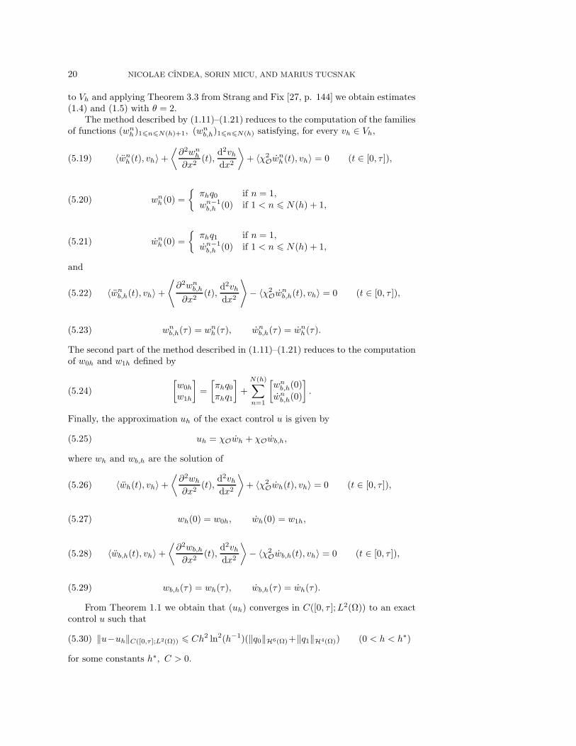
Fig. 4. The approximation uh with initial state q0(x) = x5(1−x)5, q1(x) = −q0(x) and controltime τ = 1.

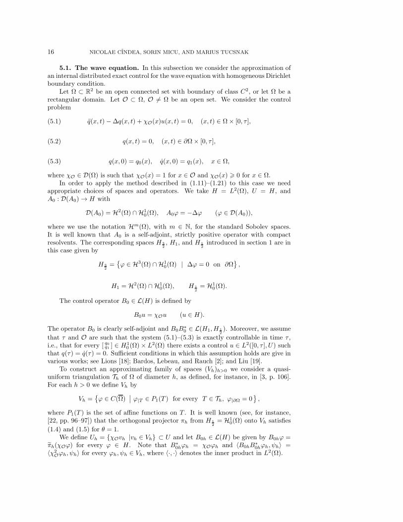
We tested the algorithm in the case O = (13 ,23 ), and the initial data that we want

to steer to zero are q0(x) = x5(1− x)5, q1(x) = −q0(x) and the control time is τ = 1.Note that [ q0q1 ] ∈ H 3

2×H1. We used N = 100 discretization points in space, and in

time we used an implicit centered-difference scheme with the CFL number equal to0.1.

Figure 3(a) shows the norm decay of the solution of the discretized beam equationcorresponding to (5.16)–(5.18), with the control uh given by (1.17). Figure 3(b)displays the dependence of the norm of the solution of (5.16)–(5.18), at time τ , onthe number N of terms used in the calculus of [w0h

w1h].

Figure 4 gives the form of the approximate control uh corresponding to the initialdata [ q0q1 ] given above.


REFERENCES

[1] G. A. Baker, Error estimates for finite element methods for second order hyperbolic equations,SIAM J. Numer. Anal., 13 (1976), pp. 564–576.

[2] C. Bardos, G. Lebeau, and J. Rauch, Sharp sufficient conditions for the observation, control,and stabilization of waves from the boundary, SIAM J. Control Optim., 30 (1992), pp. 1024–1065.

[3] S. Brenner and L. Scott, The Mathematical Theory of Finite Element Methods, Texts inAppl. Math. 15, Springer-Verlag, New York, 1994.

[4] G. Chen, Control and stabilization for the wave equation in a bounded domain, SIAM J.Control Optim., 17 (1979), pp. 66–81.

[5] B. Dehman and G. Lebeau, Analysis of the HUM control operator and exact controllabilityfor semilinear waves in uniform time, SIAM J. Control Optim., 48 (2009), pp. 521–550.

[6] S. Ervedoza and J. Valein, On the observability of abstract time-discrete linear parabolicequations, Rev. Mat. Complut., 23 (2010), pp. 163–190.

[7] S. Ervedoza and E. Zuazua, Perfectly matched layers in 1-d: Energy decay for continuousand semi-discrete waves, Numer. Math., 109 (2008), pp. 597–634.

[8] S. Ervedoza and E. Zuazua, Uniformly exponentially stable approximations for a class ofdamped systems, J. Math. Pures Appl. (9), 91 (2009), pp. 20–48.

[9] S. Ervedoza and E. Zuazua, A systematic method for building smooth controls for smoothdata, Discrete Contin. Dyn. Syst., 14 (2010), pp. 1375–1401.

[10] R. Font and F. Periago, Numerical simulation of the boundary exact control for the systemof linear elasticity, Appl. Math. Lett., 23 (2010), pp. 1021–1026.

[11] R. Glowinski, C. H. Li, and J.-L. Lions, A numerical approach to the exact boundary control-lability of the wave equation I. Dirichlet controls: Description of the numerical methods,Japan J. Appl. Math., 7 (1990), pp. 1–76.

[12] R. Glowinski and J.-L. Lions, Exact and approximate controllability for distributed parametersystems, Acta Numer., 1995, pp. 159–333.

[13] G. Haine and K. Ramdani, Reconstructing Initial Data Using Observers: Error Analysis ofthe Semi-Discrete and Fully Discrete Approximations, preprint, 2010; available online athttp://arxiv.org/abs/1008.4737.

[14] A. Haraux, Une remarque sur la stabilisation de certains systemes du deuxieme ordre entemps, Portugal. Math., 46 (1989), pp. 245–258.

[15] K. Ito, K. Ramdani, and M. Tucsnak, A time reversal based algorithm for solving initialdata inverse problems, Discrete Contin. Dyn. Syst. Ser. S, 4 (2011), pp. 641–652.

[16] S. Labbe and E. Trelat, Uniform controllability of semidiscrete approximations of paraboliccontrol systems, Systems Control Lett., 55 (2006), pp. 597–609.

[17] G. Lebeau and M. Nodet, Experimental study of the HUM control operator for linear waves,Experiment. Math., 19 (2010), pp. 93–120.

[18] J.-L. Lions, Controlabilite exacte, perturbations et stabilisation de systemes distribues. Tome1, Rech. Math. Appl. 8, Masson, Paris, 1988.

[19] K. Liu, Locally distributed control and damping for the conservative systems, SIAM J. ControlOptim., 35 (1997), pp. 1574–1590.

[20] S. Micu and M. Tucsnak, Approximate controllability of a semi-discrete 1-D wave equation,An. Univ. Craiova Ser. Mat. Inform., 32 (2005), pp. 48–58.

[21] P. Pedregal, F. Periago, and J. Villena, A numerical method of local energy decay forthe boundary controllability of time-reversible distributed parameter systems, Stud. Appl.Math., 121 (2008), pp. 27–47.

[22] A. Quarteroni and A. Valli, Numerical Approximation of Partial Differential Equations,Springer Ser. Comput. Math. 23, Springer-Verlag, Berlin, 1997.

[23] K. Ramdani, T. Takahashi, and M. Tucsnak, Uniformly exponentially stable approximationsfor a class of second order evolution equations—application to LQR problems, ESAIMControl Optim. Calc. Var., 13 (2007), pp. 503–527.

[24] R. Rebarber and G. Weiss, An extension of Russell’s principle on exact controllability, inProceedings of the Fourth European Control Conference (ECC), Brussels, Belgium, 1997.CD-ROM.

[25] D. Russell, Exact boundary value controllability theorems for wave and heat processes in star-complemented regions, in Differential Games and Control Theory (Proc. NSF—CBMSRegional Res. Conf., University of Rhode Island, Kingston, RI, 1973), Lecture Notes inPure Appl. Math. 10, Dekker, New York, 1974, pp. 291–319.

[26] D. Russell, Controllability and stabilizability theory for linear partial differential equations:Recent progress and open questions, SIAM Rev., 20 (1978), pp. 639–739.


[27] G. Strang and G. Fix, An Analysis of the Finite Element Method, Prentice-Hall Series inAutomatic Computation, Prentice-Hall Inc., Englewood Cliffs, NJ, 1973.

[28] L. T. Tebou and E. Zuazua, Uniform exponential long time decay for the space semi-discretization of a locally damped wave equation via an artificial numerical viscosity, Nu-mer. Math., 95 (2003), pp. 563–598.

[29] M. Tucsnak and G. Weiss, How to get a conservative well-posed linear system out of thin air.Part I: Well-posedness and energy balance, ESAIM Control Optim. Calc. Var., 9 (2003),pp. 247–274.

[30] M. Tucsnak and G. Weiss, How to get a conservative well-posed linear system out of thinair. Part II. Controllability and stability, SIAM J. Control Optim., 42 (2003), pp. 907–935.

[31] M. Tucsnak and G. Weiss, Observation and Control for Operator Semigroups, BirkhauserAdv. Texts Basler Lehrbucher, Birkhauser Verlag, Basel, 2009.

[32] E. Zuazua, Optimal and approximate control of finite-difference approximation schemes forthe 1D wave equation, Rend. Mat. Appl. (7), 24 (2004), pp. 201–237.

[33] E. Zuazua, Propagation, observation, and control of waves approximated by finite differencemethods, SIAM Rev., 47 (2005), pp. 197–243.

Documents

AN APPROXIMATION METHOD FOR EXACT CONTROLS OF …math.ucv.ro/~micu/auxiliare/work_ro/doc/papers/cmt.pdf · 2011-05-26 · AN APPROXIMATION METHOD FOR EXACT CONTROLS OF ... The algorithm