Accepted Manuscript

An artificial bee colony algorithm with a Modified Choice Function for the travelingsalesman problem

Shin Siang Choong, Li-Pei Wong, Chee Peng Lim

PII: S2210-6502(17)30944-6

DOI: 10.1016/j.swevo.2018.08.004

Reference: SWEVO 427

To appear in: Swarm and Evolutionary Computation BASE DATA

Received Date: 3 December 2017

Revised Date: 5 June 2018

Accepted Date: 4 August 2018

Please cite this article as: S.S. Choong, L.-P. Wong, C.P. Lim, An artificial bee colony algorithm with aModified Choice Function for the traveling salesman problem, Swarm and Evolutionary ComputationBASE DATA (2018), doi: 10.1016/j.swevo.2018.08.004.

This is a PDF file of an unedited manuscript that has been accepted for publication. As a service toour customers we are providing this early version of the manuscript. The manuscript will undergocopyediting, typesetting, and review of the resulting proof before it is published in its final form. Pleasenote that during the production process errors may be discovered which could affect the content, and alllegal disclaimers that apply to the journal pertain.

MANUSCRIP

T

ACCEPTED

ACCEPTED MANUSCRIPT

An Artificial Bee Colony Algorithm with a Modified Choice Function for the Traveling Salesman Problem

Shin Siang Choong a, Li-Pei Wong b,*, Chee Peng Lim c

a, b School of Computer Sciences, Universiti Sains Malaysia, Malaysia c, Institute for Intelligent Systems Research and Innovation, Deakin University, Australia

a css15_com047@student.usm.my, b lpwong@usm.my, c chee.lim@deakin.edu.au

Abstract

The Artificial Bee Colony (ABC) algorithm is a swarm intelligence approach which has initially been proposed to solve optimisation of mathematical test functions with a unique neighbourhood search mechanism. This neighbourhood search mechanism could not be directly applied to combinatorial discrete optimisation problems. In order to tackle combinatorial discrete optimisation problems, the employed and onlooker bees need to be equipped with problem-specific perturbative heuristics. However, a large variety of problem-specific heuristics are available, and it is not an easy task to select an appropriate heuristic for a specific problem. In this paper, a hyper-heuristic method, namely a Modified Choice Function (MCF), is applied such that it can regulate the selection of the neighbourhood search heuristics adopted by the employed and onlooker bees automatically. The Lin-Kernighan (LK) local search strategy is integrated to improve the performance of the proposed model. To demonstrate the effectiveness of the proposed model, 64 Traveling Salesman Problem (TSP) instances available in TSPLIB are evaluated. On average, the proposed model solves the 64 instances to 0.055% from the known optimum within approximately 2.7 minutes. A performance comparison with other state-of-the-art algorithms further indicates the effectiveness of the proposed model. Keywords: hyper-heuristic; metaheuristic; bee algorithm; combinatorial optimisation problem; neighbourhood search; Lin-Kernighan.

1. Introduction

A computational optimisation methodology involves finding feasible solutions from a finite set of solutions, and identifying only the optimal solution(s). Swarm intelligence algorithms constitute a sub-class of computational optimisation methodology [1]. Swarm intelligence algorithms are developed based on emergence of collective behaviours pertaining to a population of interacting individuals in adapting to the local and/or global environments. Examples of swarm intelligence algorithms include Particle Swarm

* Corresponding author. Tel.: +604-6534751 E-mail address: lpwong@usm.my

MANUSCRIP

T

ACCEPTED

ACCEPTED MANUSCRIPT 2

Optimisation (PSO) [2], Ant Colony Optimisation (ACO) [3], Bat Algorithm (BA) [4], Firefly Algorithm (FA) [5], Cuckoo Search Algorithm (CSA) [6], and bee-inspired algorithms [7-9].

Bees are highly organised social insects. Their survival relies on assigning an important task to each bee in a cooperative mode. The tasks include reproduction, foraging, and constructing hive. Within these tasks, foraging is one of the most important tasks, because the bee colony must ensure an undisrupted supply of food to survive. The food foraging behaviours of bees can be computationally realised as algorithmic tools to solve various optimisation problems.

The Artificial Bee Colony (ABC) algorithm is one of the popular bee-inspired algorithms. Proposed by Karaboga [7], it is inspired by the foraging behaviours of honey bees in a colony. In the ABC algorithm, a food source represents a possible solution to the optimisation problem in the search space, and the nectar amount of the food source represents the fitness of that solution. The ABC algorithm defines three types of bees: employed bees, onlooker bees, and scout bees. An employed bee looks for new food sources around the neighbourhood of the food source that it has previously visited. An onlooker bee observes dances and selects a food source to visit. It tends to select good food sources from those found by the employed bees. A scout bee searches for new food sources randomly.

The mechanism of the ABC algorithm is as follows. The employed bees first perform a neighbourhood search nearby the food source in their memory (i.e. solution). Then, they go back to the hive and perform dances. The dances inform the onlooker bees about the fitness of each solution. Each onlooker bee observes and selects a food source to perform another neighbourhood search based on a probability proportional to the food source fitness (i.e. a roulette wheel selection). The onlooker bees tend to select good food sources from those found by the employed bees. The employed and onlooker bees perform neighbourhood search by perturbing an existing solution to produce a new solution. A greedy approach is applied to decide whether to accept the newly perturbed solution. If a solution could not be improved after a pre-determined number of trails (denoted as the limit), it is abandoned. The employed bee associated to that non-improving solution (i.e. local optimum) is abandoned, and it becomes a scout bee. The scout bee explores the search space at random and looks for a new solution.

This ABC algorithm has been used to solve optimisation of mathematical test functions [7]. Promising results have been reported by using a number of ABC variants [10-12]. To find the optimum solution of the mathematical test functions, the neighbourhood search performed by the employed and onlooker bees is formulated as follows (Eq. (1)):

vij = xij + ϕ (xij - xkj) (1)

in which xi is the solution associated to the i-th employed bee, xij is j-th element (i.e. dimension) of solution xi, vi is the new solution produced based on xi, vij is j-th element of solution vi, j is a random integer between 1 and dim (the dimensionality of the problem), ϕ is a random real number between -1 and 1, and k is a random integer between 1 and n (the number of employed bees).

In recent years, the ABC algorithm has been modified to solve combinatorial discrete optimisation problems, such as quadratic assignment problem [13], p-median problem [14-16], minimum spanning tree problem [17-19], clustering problem [20-22], uncapacitated facility location problem [23-25], Knapsack Problem (KP) [26-28], Job Shop Scheduling Problem (JSSP) [29-31], Vehicle Routing Problem (VRP) [32, 33], and Traveling Salesman Problem (TSP) [34, 35]. However, Eq. (1) cannot be directly applied when solving this set of problems. The employed and onlooker bees are prescribed with a perturbative heuristic (or a set of perturbative heuristics) to generate new solutions. These heuristics are problem-specific, for instance, the neighbourhood search heuristics for TSP include insertion mutation, swap mutation, random 2-opt, etc. In view of the availability of a large variety of problem-specific heuristics, the key question concerning the selection of a particular heuristic has been posed in the literature in recent years. This leads to the motivation of using hyper-heuristics for tackling such problem, which is the focus of our research in improving the ABC

MANUSCRIP

T

ACCEPTED

ACCEPTED MANUSCRIPT 3

algorithm.

A hyper-heuristic is a high-level automated methodology for selecting or generating a set of heuristics [36]. The term “hyper-heuristic” was coined by Denzinger et al. [37]. There are two main hyper-heuristic categories, i.e. selection hyper-heuristic and generation hyper-heuristic [38]. These two categories can be defined as ‘heuristics to select heuristics’ and ‘heuristics to generate heuristics’, respectively [36]. Both selection and generation hyper-heuristics can be further divided into two categories based on the nature of the heuristics to be selected or generated [38], namely either constructive or perturbative hyper-heuristics. A constructive hyper-heuristic incrementally builds a complete solution from scratch. On the other hand, a perturbative hyper-heuristic iteratively improves an existing solution by performing its perturbative mechanisms. The heuristics to be selected or generated in a hyper-heuristic model are known as the low-level heuristics (LLHs).

A typical selection hyper-heuristic model consists of two levels [36]. The low level contains a problem representation, evaluation function(s), and a set of problem specific LLHs. The high level manages which LLH to use for producing a new solution(s), and then decides whether to accept the solution(s). Therefore, the high-level heuristic performs two separate tasks i.e. (i) LLH selection and (ii) move acceptance [39]. The LLH selection method is a strategy to select an appropriate LLH from a set of available alternatives during the search process. The available LLH selection methods include simple random [40], choice function [41-43], tabu search [44], harmony search [45], backtracking search algorithm [46], and a set of reinforcement learning variants [47, 48]. The move acceptance method decides whether to accept the new solution generated by the selected LLH. Examples of move acceptance methods include Only Improvement [49], All Moves [43], Simulated Annealing [50], Late Acceptance [40], and some variants of threshold-based acceptance.

Striking a balance between intensification and diversification is important for a hyper-heuristic [36, 51]. Intensification encourages a hyper-heuristic to focus on the promising LLHs, which leads to a good performance. On the other hand, diversification serves as a forgive-and-forget policy which encourages attempts on those rarely used LLHs. Both intensification and diversification are crucial components as the capability of an LLH varies during different phases of the search process [52, 53]. An LLH with a good performance in one phase should not dominate the subsequent search process, while a poor performance in one phase should not lead to a permanent discrimination of an LLH in the later phases. In this study, an LLH selection method which is based on a choice function, namely the Modified Choice Function (MCF) [42], is integrated with the ABC algorithm. Specifically, MCF is used to select the neighbourhood search heuristic deployed by the employed and onlooker bees. The reason of choosing MCF is because it is able to adaptively control the weights of its intensification and diversification components during different phases of the search process. Besides that, to enhance the performance of the proposed MCF-ABC model, it is integrated with the Lin-Kernighan (LK) local search strategy [54]. The proposed model is denoted as MCF-ABC. It is tested using benchmark TSP instances provided in TSPLIB [55].

This article starts with a description of the related work in Section 2. Section 3 presents the proposed MCF-ABC model. The results and findings including performance comparison are presented in Section 4. Finally, concluding remarks are presented in Section 5.

2. Related Work

This section describes the related work of the study. Section 2.1 focuses on the applications of bee-inspired algorithms to solve TSP (or variants of TSP). Section 2.2 reviews some hyper-heuristic models which are based on a choice function. Section 2.3 introduces some local-search-based strategies for combinatorial optimisation problems.

MANUSCRIP

T

ACCEPTED

ACCEPTED MANUSCRIPT 4

2.1. Application of the Bee-inspired Algorithms to Solve TSP

TSP is an NP-hard discrete combinatorial optimisation problem [56]. When solving a TSP, the aim is to look for the shortest Hamiltonian path, which is the route that leads a person to visit each location once and only once, and to return to the starting location with the minimum total distance [57]. Suppose that the cities are located in some geometric region that the distances between two cities obey the usual axioms of a distance function of a metric space. TSP can be modeled as an undirected weighted graph. Let G = (V, E) be an undirected weighted complete graph, in which V is a set of n cities (V = {v1,v2, . . . ,vn}) and E is a set of edges (E = {(r, s) : r, s ∈ V }). E is usually associated with a distance matrix, D = {dr,s} where dr,s refers to the distance between city r and city s. Let ∏ represents all possible permutations of set V. A solution of a TSP is to determine a permutation π ∈ ∏, which has the minimum total round trip distance, as shown in Eq. (2), in which π(i) ∈ V indicates the i-th element in π.

������ ∈ ∏ = ∑ [����,�����]+����,��������� (2)

A number of swarm intelligence algorithms have been employed to solve TSP, such as PSO [58, 59], ACO [60, 61], FA [62, 63], BA [64, 65], CSA [66, 67], and some hybrid algorithms [68-71]. In this study, we focus on bee-inspired algorithms to solve TSP. A discussion on the application of bee-inspired algorithms to solve TSP or its variants is presented. The associated neighbourhood search heuristic/mechanisms are also highlighted.

Marinakis et al. [72] proposed a Honey Bees Mating Optimisation (HBMO) model to solve TSP. The HBMO model employs a crossover heuristic and an Expanding Neighbourhood Search (ENS) method to perform neighbourhood search. The crossover heuristic is able to identify the common characteristics of the parents, while the ENS method combines multiple local search strategies, i.e. 2-opt, 2.5-opt, and 3-opt.

Wong [73] proposed a Bee Colony Optimisation (BCO) model. In the BCO model [73], a bee performs neighbourhood search on a selected dance (a solution constructed by another bee) based on a Fragmentation State Transition Rule (FSTR). The FSTR technique aids a bee in constructing a feasible solution under the influence of arc fitness and heuristic distance. Besides FSTR, the BCO model is equipped with three other components, i.e. waggle dance mechanism, local search, and pruning strategy. These components are bundled as a generic model [74] to solve multiple combinatorial optimisation problems, such as JSSP [75-77], Sequential Ordering Problem (SOP) [78], symmetric TSP [79-81], and asymmetric TSP [82].

Masutti and de Castro [9] proposed a bee-inspired algorithm known as TSPoptBees to solve TSP. The TSPoptBees model defines three types of bees, i.e. recruiter bees, scout bees, and recruited bees. The recruiter bees recruit other bees to exploit promising areas of the solution search space. Crossover heuristics are used to combine the solution associated with a recruited bee and its recruiter. The scout bees explore the search space by using mutation heuristics on randomly selected solutions from the population. Both the recruited and scout bees utilise a random method to select the heuristics.

Banharnsakun et al. [83] extended the ABC algorithm with a Greedy Subtour Crossover (GSX) heuristic [84] to solve TSP, which is denoted as ABC-GSX. Specifically, GSX is adopted as the neighbourhood search heuristic. In ABC-GSX, the new solutions generated during the neighbourhood search are further improved by using the 2-opt local search heuristic. GSX is able to improve the exploitation process of the ABC algorithm [83].

Karaboga and Gorkemli [85] proposed a combinatorial ABC algorithm to solve TSP. A Greedy Sub-tour Mutation (GSTM) heuristic serves as the neighbourhood search heuristic of the employed and onlooker bees. The resulting algorithm is denoted as ABC-GSTM. ABC-GSTM outperforms eight GA variants with different mutation operators [85].

Akay et al. [86] adopted a neighbour-based 2-opt move and a 2-opt local search in the ABC algorithm. The resulting algorithm is denoted as 2-opt ABC algorithm. During the neighbourhood search, an employed

MANUSCRIP

T

ACCEPTED

ACCEPTED MANUSCRIPT 5

or onlooker bee first performs a neighbour-based 2-opt move for the current solution. If the neighbour-based 2-opt move is not able to improve the solution, the solution undergoes a 2-opt local search. The experimental results show that the 2-opt ABC algorithm outperforms the 2-opt local search strategy.

Li et al. [87] applied an inner-over operator [88] as the neighbourhood search heuristic in ABC. The inner-over operator is a modified version of the inversion mutation. However, the selection of a sub-sequence to be inverted is related to the population, therefore the operator has some features of the crossover heuristic. The ABC algorithm with the inner-over operator outperforms the Bee Colony Optimisation in [8].

Zhong et al. [89] integrated the ABC algorithm with a threshold-based acceptance method. A new solution update equation and a greedy hybrid operator are proposed as the neighbourhood search mechanism. The new solution adds an edge based on another randomly selected solution to the current one. If the two solutions have a common edge, the edge to be added is formed based on a set of nearest cities. After an edge is added, the neighbour solutions are generated by applying reverse, insert, and swap heuristics. The best among the three solutions serves as the candidate solution. The empirical results show that the ABC algorithm with a threshold-based acceptance method outperforms that with a greedy acceptance.

Kocer and Akca [35] proposed an Improved ABC (IABC) algorithm with a loyalty and a threshold mechanisms to solve TSP. These two mechanisms form a decision making strategy which decides whether a bee serves as a worker or an onlooker. Besides that, a 2-opt local search strategy is integrated to avoid trapping in the local optimum [35].

Kıran et al. [34] analysed the effect of integrating single and multiple neighbourhood search heuristic(s) in a discrete ABC model. The heuristics include Random Swap (RS), Random Insertion (RI), Random Swap of Subsequences (RSS), Random Insertion of Subsequence (RIS), Random Reversing of Subsequence (RRS), Random Reversing Swap of Subsequences (RRSS), and Random Reversing Insertion of Subsequence (RRIS). The experiments in [34] can be divided into two categories. The first category consists of seven ABC models with a single neighbourhood search heuristic. The second category consists of two ABC models with multiple neighbourhood search heuristics (i.e. [RS, RSS, RRSS] and [RI, RIS, RRIS]). When multiple neighbourhood search heuristics are employed, a random selection strategy is applied. The empirical results show that the [RI, RIS, RRIS] model has a better performance on TSP instances with the number of cities ranging between 30 and 101. Comparatively, the RRS model performs better in two TSP instances with 225 and 280 cities.

Besides the classical TSP instances, bee-inspired algorithms have been adopted to solve different TSP variants. Karabulut and Tasgetiren [90] proposed a discrete ABC algorithm for solving the TSP with time windows (TSPTW). TSPTW involves a searching for a path with minimum cost that visits a set of cities once and returns to the starting city within a pre-defined time window (i.e. ready time and due date). A feasible solution of TSPTW requires a visit to each city to be made within the corresponding ready time and due date. A two-phase destruction and construction heuristic is adopted as the neighbourhood search heuristic in the discrete ABC algorithm proposed by Karabulut and Tasgetiren. During the destruction phase, a number of randomly selected cities are removed from the solution. In the construction phase, the NEH insertion heuristic [91] is applied to re-insert the removed cities back into the solution.

Pandiri and Singh [92] adopted the ABC algorithm for solving multiple TSP (MTSP) instances. There are more than one salesperson in an MTSP. The aim is to look for a path for each salesperson to visit the cities, subjected to a condition that each city must be visited exactly once by only one salesperson. The neighbourhood search mechanism in the ABC algorithm proposed by Pandiri and Singh [92] is as follows. Each city in a current solution has a certain probability to be copied to form a neighbourhood solution, otherwise the city is considered as an unassigned city. The unassigned cities are randomly inserted into the formed neighbourhood solution.

Pandiri and Singh [93] employed an ABC variant for solving a multi-depot TSP instance with load balancing. Besides having multiple salespersons, this problem considers multiple depots, in which each salesperson is stationed at a different depot. The task of a multi-depot TSP is to look for a route for each salesperson to start and end at his/her corresponding depot, such that each city is visited exactly once by one

MANUSCRIP

T

ACCEPTED

ACCEPTED MANUSCRIPT 6

salesperson. As such, the total distance traveled by the salespersons is minimised, and the workload among salespersons is balanced. Pandiri and Singh [93] applied a similar neighbourhood search mechanism as that in [92].

Zhong et al. [94] proposed a dynamic Tabu ABC model for solving MTSP with precedence constraints. MTSP with precedence constraints is a special case of MTSP whereby the cities need to be visited in a specific order. A dynamic Tabu list is designed to handle the constraints. Multiple probabilistic solution update mechanisms are implemented.

Based on the reviewed literatures in this section, it is noticed that bee-inspired algorithms can be integrated with a single or multiple neighbourhood search heuristic(s). This article proposes a new ABC model with multiple neighbourhood search heuristics. Specifically, the MCF is used to guide the selection of neighbourhood search heuristics (i.e. LLHs) in the proposed MCF-ABC model.

2.2. Modified Choice Function

Cowling et al. [41] proposed a hyper-heuristic based on a choice function. It is a score-based approach which measures the score of each LLH based on its previous performance. The score of each LLH is composed of three different measurements, i.e. f1, f2, and f3. The first measurement, f1, represents the recent performance of each LLH (Eq. (3)):

���ℎ�� = ∑ ���� � �!"� �!"� (3)

where hj denotes the j-th LLH, In(hj) denotes the fitness difference between the current solution and the newly proposed solution by the nth application of hj, Tn(hj) denotes the amount of time taken by the nth application of hj to propose the new solution, α∈(0,1) is a parameter which prioritises the recent performance.

The second measurement, f2, reflects the dependency between a consecutive pair of LLHs (Eq. (4)):

�#�ℎ$ , ℎ�� = ∑ %��� � �!&,!"�� �!&,!"�� (4)

where In(hk,hj) denotes the fitness difference between the current solution and the newly proposed solution by the nth consecutive application of hk and hj (i.e. hj is executed right after hk), Tn(hk,hj) denotes the amount of time taken by the nth consecutive application of hk and hj to propose the new solution, β∈(0,1) is a parameter which prioritises the recent performance. Both f1 and f2 are the intensification component of the choice function. They encourage the selection of high performance LLHs.

The third measurement, f3, records the elapsed time since the last execution of a particular LLH (Eq. (5)):

f3(hj) = τ(hj) (5)

where τ(hj) denotes the elapsed time (in seconds) since the last execution of hj. Note that f3 acts as a diversification component in the choice function. It prioritises those LLHs that have not been used for a long time.

The score of each LLH is computed as a weighted sum of the three measurements, f1, f2, and f3, as shown in Eq. (6):

F(hj) = αf1(hj) + βf2(hk, hj) + δf3(hj) (6)

where α, β and δ are the respective weights of f1, f2, and f3. In the initial model [41], these parameters were

MANUSCRIP

T

ACCEPTED

ACCEPTED MANUSCRIPT 7

statically fixed. Promising results have been reported when the proposed choice function (i.e. Eq. (6)) is paired with AM as its move acceptance method to solve the sales summit scheduling problem.

The parameters in Cowling et al. [41] need to be tuned and pre-determined. In order to have a more effective version of the hyper-heuristic, the parameters can be dynamically controlled during execution, as shown in Cowling et al. [95]. The values of α and β increase when the selected LLH is able to improve the solution. The growth is proportional to the magnitude of improvement over the previous solution. On the other hand, if the selected LLH performs a non-improving move, α and β are decreased proportionally to the fitness difference. This strategy is able to improve the model in Cowling et al. [41].

However, Drake et al. [42] stated some limitations of the strategy in Cowling et al. [95]. Firstly, rewarding/penalising the LLH proportionally to the fitness difference over the previous solution is arguable. During the early stages of optimisation, it is easier for a relatively weaker heuristic to obtain a great improvement from a poor starting solution, and a greater reward is assigned to this weaker heuristic. On the other hand, the improvement made in the later stages of optimisation is minor (due to convergence to an optimum solution, either local or global), and a lower reward is assigned. However, the improvement made in the later stages is more significant than the improvement made in the early stages, therefore this rewarding scheme might be misleading. Besides that, if no solution can achieve improvement for a number of iterations, this LLH selection method can descend into random selection due to the low α and β settings (i.e. the diversification component, f3, dominates the score). Targeted at these limitations, Drake et al. [42] proposed a variant of choice function, namely MCF, to manage its parameters. In MCF, α and β are combined as a single parameter, µ. The score, F, is computed as follows (Eq. (7)):

Ft(hj) = µt[f 1(hj) + f2(hk, hj)] + δtf3(hj) (7)

If the selected LLH yields an improvement, intensification is prioritised by setting µ to a static maximum value close to one, at the same time δ is reduced to a static minimum value close to zero. When the selected LLH fails to improve the solution, µ is penalised linearly with a lower bound of 0.01, while δ grows at the same rate. This prevents the intensification components (i.e. f1 and f2) from losing their influence too quickly. Specifically, µ and δ are computed as follows (Eq. (8) and (9)), in which d denotes the fitness difference between the newly proposed solution and the previous solution.

'(�ℎ�� = ) 0.99, � > 0./0[0.01, '(���ℎ�� − 0.01], � ≤ 0 (8)

δt(hj) = 1 - '(�ℎ�� (9)

In Section 3, the proposed model which incorporates MCF into the ABC algorithm is presented. The main function of MCF is to help the employed and onlooker bees to select an appropriate neighbourhood search heuristic (i.e. LLH).

2.3. Local-Search-based Strategies

Local search strategies have been used widely in solving many combinatorial optimisation problems. Generally, the procedure of this category of strategies consists of the following steps: 1. Randomly generate a feasible solution, S. 2. Perform a transformation on S to produce S’. 3. If S’ is found to be better than S, replace S with S’. 4. Repeat steps 2 and 3 until no improvement is observed. At this stage, S is said to be locally optimal.

MANUSCRIP

T

ACCEPTED

ACCEPTED MANUSCRIPT 8

A number of local search strategies that have been used for solving TSP include 2-opt [96], 3-opt [97], and LK local search [54].

In general, a local search strategy is able to yield a local optimal solution. However, its capability is limited to intensification, i.e., exploitation around the neighbourhood of the initial solution. One of the effective methods to increase the chance of a local search strategy to obtain the global optimal solution is to restart the search after a particular region of the search space is extensively exploited. A local search which adapts a restart mechanism is known as a Multi-start Local Search (MSLS) [98]. In MSLS, a local search is allowed to begin from different initial solutions. As such, it is able to yield a set of local optimal solutions. Ideally, the global optimum (or a near-global-optimal) solution can be found in the set of local optimal ones. Many MSLS variants have been developed to solve various combinatorial problems, such as permutation flow shop scheduling problem [99], generalised quadratic multiple KP [100], periodic VRP [101], and dynamic TSP [102].

In addition, diversification of a local search strategy can be improved by repeatedly performing a perturbation and a local search on a solution. One such method is Iterated Local Search (ILS) [103]. In ILS, an initial solution iteratively goes through a diversification phase and an intensification phase. During the diversification phase, a new solution is produced by performing a perturbation to the current solution. After that, the intensification phase is initiated to perform local search based on the newly produced solution. One ILS-based strategy for solving the TSP, i.e., the Chained Lin-Kernighan (CLK) heuristic, was proposed in [104, 105]. In the CLK heuristic, an LK local search is repeatedly performed on a TSP solution, which is followed by a double-bridge move [104] to exchange four arcs in the solution with the other four arcs. Besides TSP, ILS-based strategies have been used in various applications, i.e. variants of VRP [106, 107], bin-packing problem [108], and different scheduling problems [109-111].

Many swarm intelligence algorithms have good global search ability. As such, a balance between intensification and diversification can be achieved by integrating a local search strategy with a swarm intelligence algorithm. The usefulness of hybridising local search and swarm intelligence algorithms has been demonstrated in many publications [112-117]. Motivated by the research in this domain, the proposed MCF-ABC model is integrated with an LK local search strategy in this study. The local search takes place after each neighbourhood search performed by the employed or onlooker bees before applying the acceptance criterion.

With the inclusion of local search, the proposed MCF-ABC model has some similarities with the MSLS and ILS models. In the initialisation phase of MCF-ABC, a population of solutions is initialised to form multiple starting points of the local search process. During the activities performed by the employed and onlooker bees, each of these solutions undergoes an ILS procedure, i.e. repetitively goes through a perturbation using a selected LLH and an LK local search. During the activities performed by the scout bee, if a solution could not be improved after limit trials, a restart mechanism (i.e. a replacement of the solution with a random solution) takes place. Therefore, MCF-ABC shares some common features of MSLS during the initialisation phase and scout bee activities, while similarities between MCF-ABC and ILS are shown in the activities of the employed and onlooker bees.

3. The Proposed Model

The pseudo code of a classical discrete ABC model [34, 85] is shown in Algorithm I. The model consists of four phases: initialisation, employed bee phase, onlooker bee phase, and scout bee phase. In the initialisation phase, the maximum iteration (maxIteration), population size (popSize), the maximum number of trails of a solution (limit), and an LLH to be used for the neighbourhood search by the employed and onlooker bees (llhx) are pre-determined. Then, the solution associated to each food source is initialised randomly. The employed and onlooker bees perform neighbourhood search using an LLH determined during the initialisation phase throughout the search process.

MANUSCRIP

T

ACCEPTED

ACCEPTED MANUSCRIPT 9

Algorithm I: Pseudo code of a classical discrete ABC model.

1 Procedure ABC() //initialisation

2 Initialise maxIteration, popSize, limit and llhx 3 for i = 1 to popSize/2 4 foodSource[i] = initialiseSolutions() 5 foodSource[i].counter = 0 6 end for 7 while not reaching maxIteration do //Employed bee phase 8 for i = 1 to popSize/2 9 newSol = neighbourSeach(foodSource[i], llhx) 10 if getFitness(newSol) < getFitness(foodSource[i]) 11 foodSource[i] = newSol 12 foodSource[i].counter = 0 13 else 14 foodSource[i].counter++ 15 end if 16 end for

//Onlooker bee phase 17 for i = 1 to popSize/2 18 k = selectSolBasedOnRouletteWheelSelection(foodSource) 19 newSol = neighbourSeach(foodSource[k], llhx) 20 if getFitness(newSol) < getFitness(foodSource[k]) 21 foodSource[k] = newSol 22 foodSource[i].counter = 0 23 else 24 foodSource[i].counter++ 25 end if 26 end for

//Scout bee phase 27 for i = 1 to popSize/2 28 if foodSource[i].counter > foodSource[i].limit 29 foodSource[i] = initialiseSolutions() 30 foodSource[i].counter = 0 31 end if 32 end for 33 end while 34 end Procedure

The proposed MCF-ABC model is a bee algorithm with multiple neighbourhood search heuristics (i.e.

LLHs). The seven perturbative LLHs for TSP proposed in [34], namely, Random Insertion (RI), Random Swap (RS), Random Insertion of Subsequence (RIS), Random Swap of Subsequences (RSS), Random Reversing of Subsequence (RRS), Random Reversing Insertion of Subsequence (RRIS) and Random Reversing Swap of Subsequences (RRSS), is adopted. Besides that, the proposed MCF-ABC model also includes three additional LLHs i.e. Shuffle Subsequence (SS), Random Shuffle Insertion of Subsequence

MANUSCRIP

T

ACCEPTED

ACCEPTED MANUSCRIPT 10

(RSIS) and Random Shuffle Swap of Subsequence (RSSS). Therefore, a total of ten LLHs are adopted in the MCF-ABC model. These ten LLHs involve four main types of operations, i.e. reverse, insert, swap and shuffle. Specifically, RRS performs a reverse operation, RI and RIS perform an insert operation, RS and RRS perform a swap operation, and SS performs a shuffle operation. Among the ten LLHs, four of the LLHs (i.e. RRIS, RRSS, RSIS, and RSSS) involve combinations of two types of operations. Note that the subsequence of a TSP solution considered by RRS, RIS, RSS, SS, and the four LLHs with combined operations covers size in a range of [2:dim], where dim denotes the TSP dimension. The details of the ten LLHs are shown in Table 1.

Table 1: Details of the ten integrated LLHs in the MCF-ABC model.

Operations LLHs Description

Reverse Random Reversing of Subsequences (RRS)

Invert a randomly selected subsequence.

Insert Random Insertion (RI)

Randomly pick a city from a solution, remove it from the solution, and reinsert it to a random position of the solution.

Random Insertion of Subsequence (RIS)

Randomly pick a subsequence from a solution, remove it from the solution, and reinsert it to a random position of the solution.

Swap Random Swap (RS) Swap the position of two randomly selected cities in a solution. Random Swap of Subsequences (RSS)

Swap the position of two randomly selected subsequences in a solution.

Shuffle Shuffle Subsequence (SS) Re-order a randomly selected subsequence at random.

Combined Operations

Random Reversing Insertion of Subsequence (RRIS)

Invert a randomly selected subsequence, then remove the inverted subsequence from the solution, and reinsert it to a random position of the solution.

Random Reversing Swap of Subsequences (RRSS)

Swap the position of two randomly selected subsequences in a solution. Each of the subsequences has a 0.5 probability to be inverted.

Random Shuffle Insertion of Subsequence (RSIS)

Re-order a randomly selected subsequence at random, then remove the shuffled subsequence from the solution, and reinsert it to a random position of the solution.

Random Shuffle Swap of Subsequence (RSSS)

Swap the position of two randomly selected subsequences in a solution. Each of the subsequences has a 0.5 probability to be shuffled.

The fitness function of the proposed MCF-ABC model is formulated as the round trip distance (i.e. tour length) to visit each city once and only once, and return to the starting city (as shown in Eq. (2)). The pseudo code is shown in Algorithm II. Similar to the classical discrete ABC model, the proposed MCF-ABC model consists of four phases: initialisation, employed bee phase, onlooker bee phase, and scout bee phase. In MCF-ABC, the solution associated with each employed bee is initialised randomly. In order for an employed bee or an onlooker bee to select an appropriate LLH, it is aided by the MCF as explained in Section 2.2. Each LLH has a score, F. Each employed bee or onlooker bee selects an LLH based on the F score (lines 9 and 22 in Algorithm II). The computation of F is shown in Eq. (7). The LLH with the largest F score is selected and ties are decided randomly. After performing a neighbourhood search, the generated solution by the neighbourhood search is improved using the LK local search [54] (lines 11 and 24 in Algorithm II). Then, a greedy acceptance method is applied to decide whether to accept the newly produced solution or otherwise (lines 12-13 and 25-26 in Algorithm II). After that, the F score of the selected LLH is updated using Eq. (7) (lines 18 and 31 in Algorithm II).

While the employed bees and onlooker bees perform neighbourhood search to exploit the promising areas of the search space, the scout bees focus on exploration of a new region in the search space [10, 24, 118]. As such, the scout bees are good for avoiding local optima. However, some studies suggest that random replacement of an abandoned solution decreases the search efficiency, because an abandoned solution could contains more useful information than a random solution [119, 120]. In this article, the same mechanism as proposed in the original ABC algorithm by Karaboga [7] is applied, i.e. if a particular solution (i.e. food source) has not been improved after the limit trials, it is abandoned. The employed bee associated to the abandoned food source becomes a scout bee, and it goes to search for a new food source (i.e. solution) at

MANUSCRIP

T

ACCEPTED

ACCEPTED MANUSCRIPT 11

random. The scout bee uses a random initialisation procedure to generate a new solution (line 35 in Algorithm II).

Algorithm II: Pseudo code of the MCF-ABC model.

1 Procedure MCF-ABC() //initialisation

2 Initialise maxIteration, popSize, limit and LLHSet 3 for i = 1 to popSize/2 4 foodSource[i] = initialiseSolutions() 5 foodSource[i].counter = 0 6 end for 7 while not reaching maxIteration do //Employed bee phase 8 for i = 1 to popSize/2 9 selectedLLH = selectLLH_BasedOnMCF() 10 newSol = neighbourSeach(foodSource[i], selectedLLH) 11 localSearch(newSol) //optional 12 if getFitness(newSol) < getFitness(foodSource[i]) 13 foodSource[i] = newSol 14 foodSource[i].counter = 0 15 else 16 foodSource[i].counter++ 17 end if 18 updateChoiceFunction(selectedLLH) //eq. (7) 19 end for

//Onlooker bee phase 20 for i = 1 to popSize/2 21 k = selectSolBasedOnRouletteWheelSelection(foodSource) 22 selectedLLH = selectLLH_BasedOnMCF() 23 newSol = neighbourSeach(foodSource[k], selectedLLH) 24 localSearch(newsol) //optional 25 if getFitness(newSol) < getFitness(foodSource[k]) 26 foodSource[k] = newSol 27 foodSource[i].counter = 0 28 else 29 foodSource[i].counter++ 30 end if 31 updateChoiceFunction(selectedLLH) //eq. (7) 32 end for

//Scout bee phase 33 for i = 1 to popSize/2 34 if foodSource[i].counter > foodSource[i].limit 35 foodSource[i] = initialiseSolutions() 36 foodSource[i].counter = 0 37 end if 38 end for 39 end while 40 end Procedure

MANUSCRIP

T

ACCEPTED

ACCEPTED MANUSCRIPT 12

4. Results and Discussion

The experimental setting, experimental results, and comparison studies are presented in this section.

4.1. Experimental Settings

All experiments were conducted using a computer with multiple Intel i7-3930K 3.20 GHz processors, and with 15.6GB of memory. At any particular time, each test was executed by one processor only. The proposed MCF-ABC model is implemented in C programming language. The implementation of the LK local search is obtained from Concorde [105].

The performance of the proposed model is investigated by using benchmark TSP datasets taken from TSPLIB [55]. A total of 64 instances are used, and their dimension ranges from 101 to 85900 cities. The numerical figure appears in the problem instance name denotes the dimension of the problem, e.g. eil101 is a 101-city TSP; d493 is a 493-city TSP.

Two key performance indicators are defined to measure the performance of the proposed MCF-ABC model as follows: the percentage deviation from known optimum, δ (measured in %) and computational time (measured in seconds) to obtain the best tour length. The formula for calculating δ is stated in Eq. (10) where C* and C(�) denote the best known tour length (or optimum tour length) and the obtained tour length of a particular TSP instance respectively:

4 = 5���5∗5∗ × 100 (10)

When an instance is solved by the proposed MCF-ABC model, a total of 30 test replications are conducted. The shortest tour length produced by each replication and the computational time to obtain such tour length are recorded. This leads to the creation of C = {c1, c2, …, c30} and T = {t1, t2, …, t30}, in which C is a set of tour lengths and T is a set of computational time corresponding to the time to obtain the best tour length in C. For set C, the average of 30 tour lengths are identified and denoted as µC. Then, the average deviation percentages (i.e. δavg) from C∗ are computed using Eq. (10). For set T, the average is computed and is denoted as µT.

4.2. Parameter Tuning

There are two parameters in MCF-ABC, i.e. popSize and limit. To determine both parameters, a structured design-of-experiment technique, i.e. the face-centred central composite design (CCD) [121], is employed. All 64 TSP instances are grouped into four classes according to their dimensions. Classes A, B, and C include instances with dimensions [1:500], [501:1000], and [1001:10000], respectively, while Class D includes instances with dimension >10000. For each class, one TSP instance is selected as a representative instance for the CCD experiments. Specifically, gil262, u724, fnl4461, and rl11849 are selected as the representative instances of Classes A, B, C, and D respectively. The resulting parameter settings from these representative instances are generalised to other TSP instances within the corresponding class.

In accordance with the face-centred CCD [121], each parameter is set at three different levels, i.e. low, medium, and high, as shown in Table 2. A total of 32=9 combinations of these parameters at each level are generated. The experimental setting is illustrated in Figure 1. To have a fair comparison, all experiments are terminated after a fixed number of neighbourhood search operations (i.e. 10000 operations). For example, the experiment with popSize = 10 would be terminated after 1000 iterations, while the experiment with popSize = 20 would be terminated after 500 iterations. Table 3 shows the detailed configurations and results of the CCD design experiment.

MANUSCRIP

T

ACCEPTED

ACCEPTED MANUSCRIPT 13

Table 2: Low, medium, and high levels of popSize and limit.

Low Medium High

popSize 10 20 30

limit 100 200 300

Table 3: Effects of popSize and limit on the MCF-ABC performance.

Configuration popSize limit

δavg

Class A

gil262

Class B

u724

Class C

fnl4461

Class D

rl11849

1 10 100 0 0.039 0.225 0.472

2 10 200 0 0.007 0.213 0.447

3 10 300 0 0.026 0.222 0.576

4 20 100 0 0.031 0.277 0.608

5 20 200 0 0.012 0.232 0.575

6 20 300 0 0.016 0.258 0.584

7 30 100 0 0.054 0.272 0.655

8 30 200 0 0.029 0.238 0.647

9 30 300 0 0.039 0.284 0.676

MCF-ABC is able to solve gil262 to the known optimum using all the nine configurations of popSize and

limit. For Classes B, C, and D, the best results are achieved from the second configuration, i.e. popSize=10 and limit=200. With this configuration, popSize is set at the low level and limit is set at a medium level. Besides that, it is worth-noting that the configuration with limit=200 outperforms all other configurations with the same popSize. As such, 200 is selected for limit, which is in line with the setting in [122] as well. Based on the tuning results, MCF-ABC with popSize=10 and limit=200 is used in the following experiments to solve all 64 TSP instances.

Figure 1: A face-centred central composite design with two parameters.

MANUSCRIP

T

ACCEPTED

ACCEPTED MANUSCRIPT 14

4.3. Experimental Results of MCF-ABC

In order to examine the effect of the integrated LLH pool described in Table 1 listed in Section 3, the proposed MCF-ABC model with the ten integrated LLHs is compared with a variant denoted as MCF-ABC(4) which only integrates four LLHs with basic operations, i.e. RRS, RIS’, RSS’, and SS, whereby RIS’ and RSS’ consider subsequence with size [1:dim]. Besides, the proposed MCF-ABC model is compared with a Random-ABC model to examine the effectiveness of integrating the MCF hyper-heuristic in the ABC model. The Random-ABC model utilises the same sets of LLHs (i.e. ten LLHs) as MCF-ABC. In Random-ABC, a random strategy is used for the employed bees and onlooker bees to select an LLH for each neighbourhood search. For all the three algorithms (i.e. MCF-ABC, MCF-ABC(4), and Random-ABC), the stopping criterion is based on the pre-determined execution iterations (i.e. 1000 iterations). The average tour length (µC), average deviation percentages (δavg), and average computational time to obtain the best solution (µT) obtained by the three algorithms are shown in Table 4.

Table 4: Performance comparison of MCF-ABC, MCF-ABC(4), and Random-ABC based on 64 TSP benchmark instances.

Optimum MCF-ABC MCF-ABC(4) Random-ABC

µC δavg(%) µT(s) µC δavg(%) µT(s) µC δavg(%) µT(s)

eil101 629 629.0 0.000 0.0 629.0 0.000 0.0 629.0 0.000 0.0

lin105 14379 14379.0 0.000 0.0 14379.0 0.000 0.0 14379.0 0.000 0.0

pr107 44303 44303.0 0.000 0.0 44303.0 0.000 0.0 44303.0 0.000 0.0

gr120 6942 6942.0 0.000 0.0 6942.0 0.000 0.0 6942.0 0.000 0.0

pr124 59030 59030.0 0.000 0.1 59030.0 0.000 0.1 59030.0 0.000 0.1

bier127 118282 118282.0 0.000 0.1 118282.0 0.000 0.1 118282.0 0.000 0.1

ch130 6110 6110.0 0.000 0.0 6110.0 0.000 0.0 6110.0 0.000 0.0

pr136 96772 96772.0 0.000 0.2 96772.0 0.000 0.1 96772.0 0.000 0.1

gr137 69853 69853.0 0.000 0.0 69853.0 0.000 0.1 69853.0 0.000 0.1

pr144 58537 58537.0 0.000 1.8 58537.0 0.000 2.2 58537.0 0.000 1.4

ch150 6528 6528.0 0.000 0.0 6528.0 0.000 0.1 6528.0 0.000 0.0

kroB150 26130 26524.0 0.000 0.0 26524.0 0.000 0.1 26524.0 0.000 0.0

kroA200 29368 26130.0 0.000 0.1 26130.0 0.000 0.2 26130.0 0.000 0.1

pr152 73682 73682.0 0.000 1.8 73682.0 0.000 2.0 73682.0 0.000 1.1

u159 42080 42080.0 0.000 0.0 42080.0 0.000 0.0 42080.0 0.000 0.0

si175 21407 21407.0 0.000 0.2 21407.0 0.000 0.2 21407.0 0.000 0.1

brg180 1950 1950.0 0.000 0.0 1950.0 0.000 0.0 1950.0 0.000 0.0

rat195 2323 2323.0 0.000 0.2 2323.0 0.000 0.2 2323.0 0.000 0.1

d198 15780 15780.0 0.000 1.3 15780.0 0.000 1.2 15780.0 0.000 0.9

kroA200 29368 29368.0 0.000 0.1 29368.0 0.000 0.1 29368.0 0.000 0.0

kroB200 29437 29437.0 0.000 0.0 29437.0 0.000 0.1 29437.0 0.000 0.0

gr202 40160 40160.0 0.000 0.6 40160.0 0.000 0.9 40160.0 0.000 0.5

MANUSCRIP

T

ACCEPTED

ACCEPTED MANUSCRIPT 15

Optimum MCF-ABC MCF-ABC(4) Random-ABC

µC δavg(%) µT(s) µC δavg(%) µT(s) µC δavg(%) µT(s)

tsp225 3916 126643.0 0.000 0.0 126643.0 0.000 0.1 126643.0 0.000 0.0

ts225 126643 3916.0 0.000 0.1 3916.0 0.000 0.1 3916.0 0.000 0.1

pr226 80369 80369.0 0.000 1.4 80369.0 0.000 3.4 80369.0 0.000 2.1

gr229 134602 134602.0 0.000 0.8 134602.0 0.000 1.3 134602.0 0.000 0.9

gil262 2378 2378.0 0.000 0.1 2378.0 0.000 0.2 2378.0 0.000 0.1

pr264 49135 49135.0 0.000 0.1 49135.0 0.000 0.1 49135.0 0.000 0.1

a280 2579 2579.0 0.000 0.0 2579.0 0.000 0.0 2579.0 0.000 0.0

pr299 48191 48191.0 0.000 0.2 48191.0 0.000 0.2 48191.0 0.000 0.2

lin318 42029 42029.0 0.000 1.5 42029.0 0.000 4.4 42029.0 0.000 1.6

rd400 15281 15281.0 0.0002 2.4 15281.0 0.000 4.1 15281.0 0.000 2.2

fl417 11861 11861.0 0.000 5.7 11861.0 0.000 4.8 11861.0 0.000 6.3

gr431 171414 171414.0 0.000 13.0 171414.0 0.000 15.1 171414.0 0.000 12.7

pr439 107217 107217.0 0.000 2.3 107217.0 0.000 2.7 107217.0 0.000 2.2

pcb442 50778 50778.0 0.000 1.6 50778.0 0.000 1.3 50778.0 0.000 1.5

d493 35002 35002.7 0.002 20.9 35002.9 0.002 21.6 35002.7 0.002 15.8

att532 27686 27686.5 0.002 11.4 27686.9 0.003 12.6 27686.7 0.003 11.9

ali535 202339 202339.0 0.000 10.6 202339.0 0.000 9.5 202339.0 0.000 8.4

si535 48450 48498.3 0.100 53.3 48535.1 0.176 55.2 48508.1 0.120 47.4

pa561 2763 2763.1 0.004 7.1 2763.3 0.011 7.5 2763.3 0.010 8.3

u574 36905 36905.0 0.000 2.1 36905.0 0.000 3.5 36905.0 0.000 3.6

rat575 6773 6774.3 0.020 6.3 6774.4 0.021 5.8 6774.3 0.020 5.5

p654 34643 34643.0 0.000 21.5 34643.0 0.000 19.2 34643.0 0.000 21.2

d657 48912 48915.1 0.006 15.5 48913.5 0.003 14.9 48914.1 0.004 11.9

gr666 294358 294404.1 0.016 32.1 294396.8 0.013 32.8 294389.7 0.011 31.8

u724 41910 41916.5 0.016 12.9 41917.4 0.018 12.9 41916.5 0.015 14.0

rat783 8806 8806.0 0.000 4.2 8806.0 0.000 6.5 8806.0 0.000 4.1

dsj1000 18659688 18661580.6 0.010 53.2 18663249.7 0.019 60.3 18662940.7 0.017 46.9

pr1002 259045 259073.0 0.011 16.6 259231.0 0.072 25.1 259173.4 0.050 29.7

si1032 92650 92650.0 0.000 4.4 92650.0 0.000 11.2 92650.0 0.000 5.5

vm1084 239297 239322.3 0.011 24.3 239321.6 0.010 21.5 239328.5 0.013 33.3

pcb1173 56892 56897.9 0.010 15.4 56899.0 0.012 12.1 56896.7 0.008 16.3

d1291 50801 50843.7 0.084 15.7 52383.2 3.115 49.3 51963.7 2.289 68.4

d1655 62128 62221.6 0.151 27.0 62246.9 0.191 37.8 62210.2 0.132 51.6

u1817 57201 57354.2 0.268 24.6 57377.6 0.309 22.7 57359.5 0.277 40.8

MANUSCRIP

T

ACCEPTED

ACCEPTED MANUSCRIPT 16

Optimum MCF-ABC MCF-ABC(4) Random-ABC

µC δavg(%) µT(s) µC δavg(%) µT(s) µC δavg(%) µT(s)

u2152 64253 64426.5 0.270 28.3 64433.9 0.282 28.7 64415.2 0.252 39.2

pr2392 378032 378549.6 0.137 28.9 378418.2 0.102 43.1 378559.5 0.140 41.0

fl3795 28772 28825.1 0.184 131.7 32294.8 12.244 258.2 31084.0 8.036 275.6

fnl4461 182566 183002.8 0.239 66.6 183019.3 0.248 48.7 183008.5 0.242 51.3

rl5915 565530 567990.2 0.435 94.2 573022.9 1.325 109.4 572285.2 1.194 109.4

pla7397 23260728 23324321.9 0.273 247.6 23328860.6 0.293 228.0 23323272.4 0.269 191.9

rl11849 923288 928015.1 0.512 308.9 934773.2 1.244 348.9 933587.4 1.116 368.5

pla85900 142382641 143484917.5 0.774 9082.5 144037897.2 1.163 5804.8 143851971.1 1.032 6453.7

Average: 0.055 162.6 0.326 115.0 0.238 125.7

The average scores of δavg obtained by MCF-ABC, MCF-ABC(4), and Random-ABC in Table 4 are

0.055%, 0.326%, and 0.238%, respectively. On average, MCF-ABC yields better δavg than those of MCF-ABC(4) and Random-ABC. MCF-ABC solves all 64 instances to 0.055% from the known optimum within 2.7 minutes (≈162.6s). Besides that, MCF-ABC is able to consistently solve 40 out of 64 instances (i.e. 62.5%) to the known optimum for 30 replications.

To statistically compare the performance of each algorithm, the Wilcoxon signed-rank test [123] with 95% confidence interval is employed. In the Wilcoxon signed rank test, the difference between the δavg obtained by two compared algorithms is ranked. The tie instances are discarded, and N denotes the effective sample size (i.e. number of instances) after discarding the ties instances. The sum of ranks for the instances in which MCF-ABC outperforms its competitor is denoted as R+, while R- denotes the sum of ranks for the instances in which MCF-ABC is inferior to its competitor. According to the Wilcoxon signed rank test, the test statistic, W is compared with a critical value, Wcri,N [123]. W≤WCri,N indicates that there is a significant difference between the performance of the two algorithms, while W>WCri,N indicates otherwise. The results of the Wilcoxon signed ranks test are summarised in Table 5.

Table 5: The Wilcoxon signed ranked test for the comparison of MCF-ABC, MCF-ABC(4), and Random-ABC.

Comparisons (MCF-ABC vs …) N R+ R- W WCri,N Significant Difference

MCF-ABC(4) 22 226 27 27 65 yes

Random-ABC 21 177 54 54 58 yes

The Wilcoxon signed rank test results show that, the proposed MCF-ABC model significantly outperforms

MCF-ABC(4) and Random-ABC. The comparison with MCF-ABC(4) shows that the inclusion of more LLHs has positive effects on the performance, while the comparison with Random-ABC indicates that the MCF selection method performs better than the random selection method.

A convergence analysis is conducted based on a problem with the largest dimension in TSPLIB, i.e. pla85900. The best-so-far δ (computed using Eq. (10)) obtained in each iteration of the three algorithms are plotted in Figure 2. As shown in Figure 2, MCF-ABC(4) with four LLHs converges rapidly, but it is trapped in a local optimum, while Random-ABC and MCF-ABC with ten LLHs are more capable of escaping the local optimum. On the other hand, the proposed MCF-ABC model converges to a better solution than those of MCF-ABC(4) and Random-ABC in the later stage of the search process.

MANUSCRIP

T

ACCEPTED

ACCEPTED MANUSCRIPT 17

Figure 2: Convergence graph of MCF-ABC, MCF-ABC(4), and Random-ABC when solving pla85900.

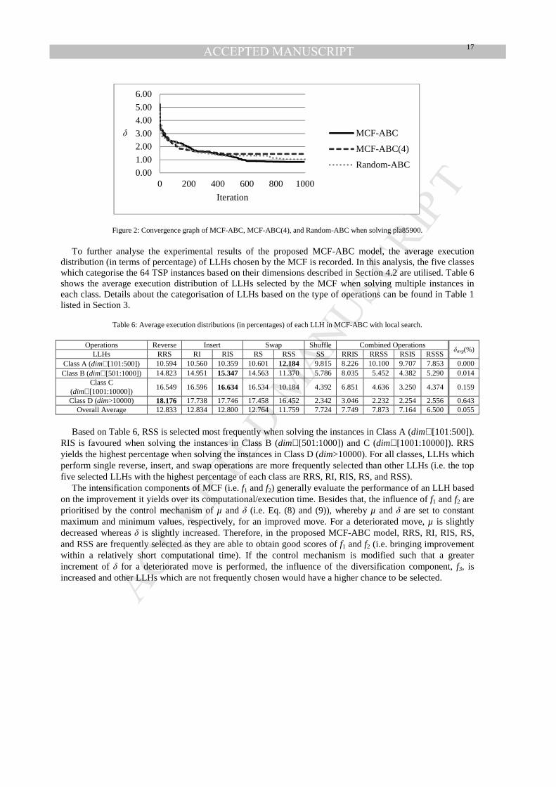
To further analyse the experimental results of the proposed MCF-ABC model, the average execution distribution (in terms of percentage) of LLHs chosen by the MCF is recorded. In this analysis, the five classes which categorise the 64 TSP instances based on their dimensions described in Section 4.2 are utilised. Table 6 shows the average execution distribution of LLHs selected by the MCF when solving multiple instances in each class. Details about the categorisation of LLHs based on the type of operations can be found in Table 1 listed in Section 3.

Table 6: Average execution distributions (in percentages) of each LLH in MCF-ABC with local search.

Operations Reverse Insert Swap Shuffle Combined Operations δavg(%)

LLHs RRS RI RIS RS RSS SS RRIS RRSS RSIS RSSS Class A (dim∈[101:500]) 10.594 10.560 10.359 10.601 12.184 9.815 8.226 10.100 9.707 7.853 0.000 Class B (dim∈[501:1000]) 14.823 14.951 15.347 14.563 11.370 5.786 8.035 5.452 4.382 5.290 0.014

Class C (dim∈[1001:10000])

16.549 16.596 16.634 16.534 10.184 4.392 6.851 4.636 3.250 4.374 0.159

Class D (dim>10000) 18.176 17.738 17.746 17.458 16.452 2.342 3.046 2.232 2.254 2.556 0.643 Overall Average 12.833 12.834 12.800 12.764 11.759 7.724 7.749 7.873 7.164 6.500 0.055

Based on Table 6, RSS is selected most frequently when solving the instances in Class A (dim∈[101:500]).

RIS is favoured when solving the instances in Class B (dim∈[501:1000]) and C (dim∈[1001:10000]). RRS yields the highest percentage when solving the instances in Class D (dim>10000). For all classes, LLHs which perform single reverse, insert, and swap operations are more frequently selected than other LLHs (i.e. the top five selected LLHs with the highest percentage of each class are RRS, RI, RIS, RS, and RSS).

The intensification components of MCF (i.e. f1 and f2) generally evaluate the performance of an LLH based on the improvement it yields over its computational/execution time. Besides that, the influence of f1 and f2 are prioritised by the control mechanism of µ and δ (i.e. Eq. (8) and (9)), whereby µ and δ are set to constant maximum and minimum values, respectively, for an improved move. For a deteriorated move, µ is slightly decreased whereas δ is slightly increased. Therefore, in the proposed MCF-ABC model, RRS, RI, RIS, RS, and RSS are frequently selected as they are able to obtain good scores of f1 and f2 (i.e. bringing improvement within a relatively short computational time). If the control mechanism is modified such that a greater increment of δ for a deteriorated move is performed, the influence of the diversification component, f3, is increased and other LLHs which are not frequently chosen would have a higher chance to be selected.

0.00

1.00

2.00

3.00

4.00

5.00

6.00

0 200 400 600 800 1000

δ

Iteration

MCF-ABC

MCF-ABC(4)

Random-ABC

MANUSCRIP

T

ACCEPTED

ACCEPTED MANUSCRIPT 18

Besides that, an experiment that excludes the LK local search is conducted to investigate the execution

distribution of LLHs in MCF-ABC without the local search strategy. The results are presented in Table 7. When the local search is excluded, the distributions of the selected LLHs for solving different classes of TSP instances are similar. MCF tends to concentrate on selecting RRS and RI, while other LLHs has less chance to be selected.

Table 7: Average execution distributions (in percentages) of each LLH in MCF-ABC without local search .

Operations Reverse Insert Swap Shuffle Combined Operations δavg(%)

LLHs RRS RI RIS RS RSS SS RRIS RRSS RSIS RSSS Class A (dim∈[101:500]) 74.958 23.252 0.731 0.105 0.077 0.059 0.666 0.095 0.030 0.026 5.498 Class B (dim∈[501:1000]) 71.239 26.104 1.075 0.149 0.112 0.072 1.035 0.138 0.040 0.035 10.115

Class C (dim∈[1001:10000]) 70.836 28.564 0.199 0.024 0.019 0.011 0.311 0.023 0.006 0.005 18.061 Class D (dim>10000) 60.086 38.974 0.467 0.011 0.013 0.004 0.427 0.013 0.003 0.002 23.361

Overall Average 72.952 25.395 0.665 0.092 0.068 0.049 0.644 0.084 0.026 0.022 9.474

4.4. Competitiveness of MCF-ABC

This section compares the proposed MCF-ABC model with state-of-the-art algorithms. The comparison is conducted based on the following publications (the abbreviation of each publication is shown in parentheses): • The analysis of discrete artificial bee colony algorithm with neighbourhood operator on traveling salesman

problem (ABC) [34]. • A hierarchic approach based on swarm intelligence to solve the traveling salesman problem (ACO-ABC)

[70]. • 2-opt based artificial bee colony algorithm for solving traveling salesman problem (2-opt ABC) [86]. • TSPoptBees: A bee-Inspired algorithm to solve the traveling salesman problem (TSPoptBees) [9]. • A generic bee colony optimisation framework for combinatorial optimisation problems (BCO) [73]. • Hybrid discrete artificial bee colony algorithm with threshold acceptance criterion for traveling salesman

problem (HDABC) [89]. • Chained lin-kernighan for large traveling salesman problems (CLK) [105]. • Effective heuristics for ant colony optimisation to handle large-scale problems (ESACO) [60]. • Quantum inspired particle swarm combined with lin-kernighan-helsgaun method to the traveling salesman

problem (QPSO) [115]. • Honey bees mating optimisation algorithm for the Euclidean traveling salesman problem (HBMO) [72].

In order to have a fair comparison, the maxIteration of the proposed MCF-ABC are set such that it uses

equal or less number of neighbourhood search operations as compared with the benchmark algorithm (if stated) as shown in Table 8. Note that a ceiling function (i.e. ⌈Dim/2⌉) is used to determine popSize in [34] and [70]. For example, if the problem is eil51, the value of popSize is ⌈51/2⌉=⌈25.5⌉=26. In ACO-ABC [70], each of the ACO and ABC algorithms is executed for 250 iterations. TSPoptBees uses a dynamic population size, and its stopping criteria are based on the maximum number of iterations without improvement. The average final popSize and maxIteration for each instance are reported in Masutti and de Castro [9]. The average final popSize is varied between 99.60 and 177.00, while the average maxIteration used is varied between 1155.83 and 4271.83. As the source code of CLK [105] is available in the Concorde TSP solver software∗, CLK is re-

∗ Available: http://www.math.uwaterloo.ca/tsp/concorde/

MANUSCRIP

T

ACCEPTED

ACCEPTED MANUSCRIPT 19

executed on the TSP instances in Classes C and D (as defined in Section 4.2) for comparison. CLK is a single-solution-based model (popSize=1), and it is allowed to run for 10,000 iterations. Except this maximum iteration, the default settings in Concorde are retained for other configurations, which include the level of backtracking (i.e. (4, 3, 3, 2)-breadth), choice of the kick (i.e. 50-step random-walk kick), and the initialisation method (i.e. Quick-Boruvka). For the comparison with ABC [34], ACO-ABC [70], 2-opt ABC [86], TSPoptBees [9], BCO [73], HDABC [89], and CLK [105], the maxIteration of MCF-ABC is set to 1000, while for the comparison with ESACO [60], QPSO [115], and HBMO [72], it is set to 300, 10000, and 5000 respectively. The δavg results obtained by the benchmark algorithms are shown in Tables 9-17. The Wilcoxon signed rank test with 95% confidence interval is conducted for statistical comparison between MCF-ABC and each benchmark algorithm.

Table 8: Experimental settings used by the compared algorithms and the proposed MCF-ABC model.

Approaches [Citation]

Experimental Settings

Benchmark Algorithms MCF-ABC

maxIteration popSize maxIteration popSize ABC [34] 100000 ⌈Dim/2⌉×2

1000 10

ACO-ABC [70] 250+250 ⌈Dim/2⌉×2

2-opt ABC [86] 40 2000

TSPoptBees [9] varied from 1155.83 to 4271.83 varied from 99.60 to 177.00

BCO [73] 10000 50

HDABC [89] 1000 30

CLK [105] 10000 1

ESACO [60] 300 10 300 10

HBMO [72] 1000 50 5000 10

QPSO [115] 1000 100 10000 10

Table 9: Performance comparison among MCF-ABC and nine ABC variants [34].

oliver30 eil51 berlin52 st70 pr76 kroA100 eil101 tsp225 a280

ABC [RS] 12.77 18.06 21.64 37.01 36.10 58.61 30.37 87.08 118.12

ABC [RSS] 0.00 0.50 0.24 1.48 1.58 3.74 5.22 26.12 42.46

ABC [RI] 4.88 8.02 11.29 14.21 15.04 21.47 12.78 27.40 38.04

ABC [RIS] 0.03 1.61 0.62 1.59 1.71 3.35 5.06 22.32 36.80

ABC [RRS] 0.33 2.59 3.05 2.67 1.53 2.63 5.30 8.07 11.27

ABC [RRIS] 0.00 0.35 0.00 0.55 0.62 1.89 3.51 21.62 33.48

ABC [RRSS] 0.00 0.32 0.00 0.80 0.64 1.89 3.59 20.93 38.01

ABC [RS, RSS, RRSS] 0.00 0.28 0.04 1.04 0.93 2.17 3.93 19.83 31.72

ABC [RI, RIS, RRIS] 0.00 0.39 0.00 0.56 0.45 1.04 2.90 12.41 23.92

MCF-ABC 0.00 0.00 0.00 0.00 0.00 0.00 0.00 0.00 0.00

MANUSCRIP

T

ACCEPTED

ACCEPTED MANUSCRIPT 20

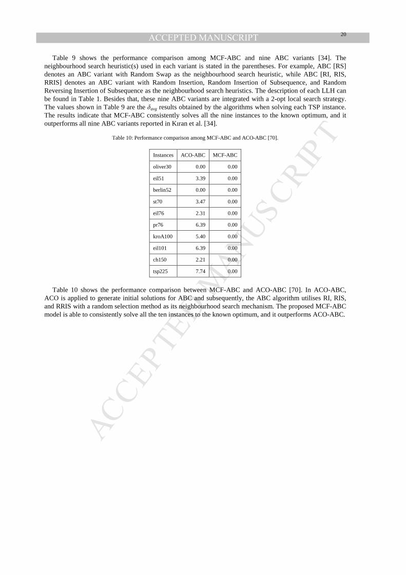
Table 9 shows the performance comparison among MCF-ABC and nine ABC variants [34]. The

neighbourhood search heuristic(s) used in each variant is stated in the parentheses. For example, ABC [RS] denotes an ABC variant with Random Swap as the neighbourhood search heuristic, while ABC [RI, RIS, RRIS] denotes an ABC variant with Random Insertion, Random Insertion of Subsequence, and Random Reversing Insertion of Subsequence as the neighbourhood search heuristics. The description of each LLH can be found in Table 1. Besides that, these nine ABC variants are integrated with a 2-opt local search strategy. The values shown in Table 9 are the δavg results obtained by the algorithms when solving each TSP instance. The results indicate that MCF-ABC consistently solves all the nine instances to the known optimum, and it outperforms all nine ABC variants reported in Kıran et al. [34].

Table 10: Performance comparison among MCF-ABC and ACO-ABC [70].

Instances ACO-ABC MCF-ABC

oliver30 0.00 0.00

eil51 3.39 0.00

berlin52 0.00 0.00

st70 3.47 0.00

eil76 2.31 0.00

pr76 6.39 0.00

kroA100 5.40 0.00

eil101 6.39 0.00

ch150 2.21 0.00

tsp225 7.74 0.00

Table 10 shows the performance comparison between MCF-ABC and ACO-ABC [70]. In ACO-ABC,

ACO is applied to generate initial solutions for ABC and subsequently, the ABC algorithm utilises RI, RIS, and RRIS with a random selection method as its neighbourhood search mechanism. The proposed MCF-ABC model is able to consistently solve all the ten instances to the known optimum, and it outperforms ACO-ABC.

MANUSCRIP

T

ACCEPTED

ACCEPTED MANUSCRIPT 21

Table 11: Performance comparison between MCF-ABC and TSPoptBees [9].

Instances TSPoptBees MCF-ABC Instances TSPoptBees MCF-ABC

att48 0.33 0.00 lin105 0.43 0.00

eil51 0.72 0.00 pr107 0.36 0.00

berlin52 0.32 0.00 pr124 0.84 0.00

st70 0.87 0.00 bier127 0.36 0.00

eil76 1.26 0.00 pr136 2.98 0.00

pr76 0.43 0.00 kroA150 1.51 0.00

kroA100 0.35 0.00 kroB150 1.54 0.00

kroB100 0.66 0.00 rat195 1.69 0.00

kroC100 0.70 0.00 kroA200 0.98 0.00

kroD100 1.18 0.00 kroB200 2.25 0.00

kroE100 0.57 0.00 tsp225 2.25 0.00

rd100 1.66 0.00 a280 2.02 0.00

eil101 0.77 0.00 lin318 2.34 0.00

Table 11 shows the performance comparison between MCF-ABC and TSPoptBees [9]. MCF-ABC is able

to obtain better δavg as compared with TSPoptBees for all instances. Besides that, MCF-ABC consistently solves all the 26 instances to the known optimum for 30 replications.

MANUSCRIP

T

ACCEPTED

ACCEPTED MANUSCRIPT 22

Table 12: Performance comparison between MCF-ABC and BCO [73].

Instances BCO MCF-ABC Instances BCO MCF-ABC

eil101 0.000 0.000 pr299 0.029 0.000

lin105 0.000 0.000 lin318 0.159 0.000

pr107 0.000 0.000 rd400 0.229 0.000

gr120 0.078 0.000 fl417 0.130 0.000

pr124 0.000 0.000 gr431 0.582 0.000

bier127 0.000 0.000 pr439 0.041 0.000

ch130 0.000 0.000 pcb442 0.423 0.000

pr136 0.018 0.000 d493 0.354 0.002

gr137 0.000 0.000 att532 0.351 0.002

pr144 0.000 0.000 ali535 0.103 0.000

ch150 0.000 0.000 si535 0.034 0.100

kroA150 0.000 0.000 pa561 0.948 0.004

kroB150 0.000 0.000 u574 0.697 0.000

pr152 0.000 0.000 rat575 0.537 0.020

u159 0.000 0.000 p654 0.048 0.000

si175 0.000 0.000 d657 0.445 0.006

rat195 0.198 0.000 gr666 0.553 0.016

d198 0.072 0.000 u724 0.622 0.016

kroA200 0.000 0.000 rat783 0.895 0.000

kroB200 0.002 0.000 pr1002 0.853 0.011

gr202 0.027 0.000 si1032 0.000 0.000

ts225 0.000 0.000 vm1084 0.495 0.011

tsp225 0.000 0.000 pcb1173 0.924 0.010

pr226 0.000 0.000 d1291 0.447 0.084

gr229 0.010 0.000 d1655 1.062 0.151

gil262 0.000 0.000 u1817 1.356 0.268

pr264 0.000 0.000 u2152 1.496 0.270

a280 0.000 0.000 pr2392 1.044 0.137

Table 12 shows the performance comparison between MCF-ABC and BCO [73]. MCF-ABC obtains better

δavg than BCO for 33 instances, while BCO outperforms MCF-ABC in solving si535. MCF-ABC is able to consistently solve 39 out of 56 instances to the known optimum as compared with 22 out of 56 instances by BCO.

MANUSCRIP

T

ACCEPTED

ACCEPTED MANUSCRIPT 23

Table 13: Performance comparison between MCF-ABC and HDABC [89].

Instances HDABC MCF-ABC Instances HDABC MCF-ABC

eil101 0.05 0.00 lin318 0.26 0.00

pr107 0.10 0.00 rd400 0.26 0.00

pr124 0.00 0.00 gr431 1.01 0.00

pr144 0.02 0.00 pr439 0.22 0.00

ch150 0.31 0.00 pcb442 0.15 0.00

kroA150 0.05 0.00 u574 0.37 0.00

pr152 0.00 0.00 rat575 0.75 0.02

rat195 0.61 0.00 u724 0.33 0.02

d198 0.27 0.00 rat783 0.91 0.00

kroA200 0.05 0.00 pr1002 0.71 0.01

kroB200 0.02 0.00 pcb1173 0.77 0.01

ts225 0.00 0.00 d1291 1.64 0.08

pr226 0.00 0.00 d1655 1.28 0.15

gr229 0.38 0.00 fnl4461 1.30 0.24

gil262 0.00 0.00 pla7397 1.47 0.27

pr264 0.00 0.00 pla85900 2.23 0.77

pr299 0.06 0.00

Table 13 shows the performance comparison between MCF-ABC and HDABC [89]. MCF-ABC obtains

better δavg than HDABC for 27 instances. For the other six instances, both MCF-ABC and HDABC obtain δavg=0.00. MCF-ABC is able to solve 23 out of 33 instances to the known optimum, as compared with 6 out of 33 instances by HDABC.

Table 14: Performance comparison between MCF-ABC and CLK [105].

Instances CLK MCF-ABC Instances CLK MCF-ABC

pr1002 0.126 0.011 pr2392 0.283 0.137

si1032 0.005 0.000 fl3795 0.732 0.184

vm1084 0.038 0.011 fnl4461 0.145 0.239

pcb1173 0.041 0.010 rl5915 0.277 0.435

d1291 0.216 0.084 pla7397 0.275 0.273

d1655 0.170 0.151 rl11849 0.409 0.512

u1817 0.361 0.268 pla85900 0.698 0.774

u2152 0.546 0.270

Table 14 shows the performance comparison between MCF-ABC and CLK [105]. MCF-ABC and CLK

employ the same implementation of the LK local search strategy. Comparing with CLK, MCF-ABC obtains

MANUSCRIP

T

ACCEPTED

ACCEPTED MANUSCRIPT 24

better δavg in solving smaller-scale instances (dim≤3795). However, CLK outperforms MCF-ABC for larger-scale instances, i.e. fnl4461, pla7397, rl11849, and pla85900.

Table 15: Performance comparison between MCF-ABC and ESACO [60].

Instances ESACO MCF-ABC Instances ESACO MCF-ABC

lin105 0.000 0.000 rat783 0.043 0.000

d198 0.000 0.000 pr1002 0.179 0.007

kroA200 0.000 0.000 fl3795 0.388 0.178

a280 0.004 0.000 fnl4461 0.482 0.215

lin318 0.059 0.000 rl5915 0.669 0.439

pcb442 0.050 0.000 pla7397 0.553 0.233

att532 0.055 0.004 rl11849 0.764 0.479

Table 15 shows the performance comparison between MCF-ABC and ESACO [60]. Both MCF-ABC and

ESACO are able to solve lin105, d198 and kroA200 to the known optimum. However, for the TSP instances with dim>200, MCF-ABC outperforms ESACO. MCF-ABC is able to solve 7 out of 14 instances to the known optimum within 3000 neighbourhood search operations as compared with 3 out of 14 instances by ESACO.

Table 16: Performance comparison between MCF-ABC and QPSO [115].

Instances QPSO MCF-ABC Instances QPSO MCF-ABC

swiss42 0.000 0.000 pr1002 0.000 0.000

gr229 0.010 0.000 pcb1173 0.002 0.000

pcb442 0.000 0.000 d1291 0.096 0.010

gr666 0.029 0.003 u1817 0.073 0.136

dsj1000 0.026 0.003 fl3795 0.025 0.022

Table 16 shows the performance comparison between MCF-ABC and QPSO [115]. Both MCF-ABC and

QPSO employ an LK-based local search. MCF-ABC obtains better or equal δavg as compared with QPSO in solving all the ten instances except u1817. MCF-ABC is able to solve 5 out of 10 instances to the known optimum within 10000 neighbourhood search operations as compared with 3 out of 10 instances by QPSO.

MANUSCRIP

T

ACCEPTED

ACCEPTED MANUSCRIPT 25

Table 17: Performance comparison between MCF-ABC and HBMO [72].

Instances HBMO MCF-ABC Instances HBMO MCF-ABC

eil101 0.000 0.000 pr439 0.000 0.000

lin105 0.000 0.000 pcb442 0.000 0.000

pr107 0.000 0.000 d493 0.000 0.000

pr124 0.000 0.000 rat575 0.000 0.007

bier127 0.000 0.000 p654 0.000 0.000

ch130 0.000 0.000 d657 0.000 0.002

pr136 0.000 0.000 rat783 0.000 0.000

pr144 0.000 0.000 dsj1000 0.012 0.004

ch150 0.000 0.000 pr1002 0.001 0.000

kroA150 0.000 0.000 vm1084 0.005 0.007

pr152 0.000 0.000 pcb1173 0.003 0.000

rat195 0.000 0.000 d1291 0.000 0.042

d198 0.000 0.000 d1655 0.122 0.008

kroA200 0.000 0.000 u1817 0.028 0.172

kroB200 0.000 0.000 u2152 0.390 0.140

ts225 0.000 0.000 pr2392 0.028 0.027

pr226 0.000 0.000 fl3795 0.370 0.041

gil262 0.000 0.000 fnl4461 0.350 0.121

pr264 0.000 0.000 rl5915 0.012 0.186

a280 0.000 0.000 pla7397 0.009 0.132

pr299 0.000 0.000 rl11849 0.098 0.273

rd400 0.000 0.000 pla85900 0.210 0.447

fl417 0.000 0.000

Table 17 shows the performance comparison between MCF-ABC and HBMO [72]. The local search

strategy employed by HBMO is known as ENS. ENS is similar to the LK local search because they both use multiple neighbourhood structures. For the instances with smaller dimensions (i.e. dim<500), both MCF-ABC and HBMO are able to yield the known optimum within 5000 neighbourhood search operations. MCF-ABC outperforms HBMO in solving several medium-scale instances, i.e. u2152, pr2392, fl3795, and fnl4461. However, for larger-scale instances, i.e. rl5915, pla7397, rl11849, and pla85900, HBMO yields better δavg as compared with MCF-ABC.

To statistically compare the overall performance of MCF-ABC and other algorithms, the Wilcoxon signed rank test with 95% confidence interval is employed. The results of the Wilcoxon signed ranks test are summarised in Table 18. Table 18 indicates that, based on the 95% confidence interval, the proposed MCF-ABC model significantly outperforms 15 algorithms, with W≤WCri,N and R+>R-. Besides, it is comparable with CLK, QPSO and HBMO (W>WCri,N).

MANUSCRIP

T

ACCEPTED

ACCEPTED MANUSCRIPT 26

Table 18: The Wilcoxon signed ranked test for the comparison of MCF-ABC and state-of-the-art algorithms.

Comparisons (MCF-ABC vs …) Citation N R+ R- W WCri,N Significant Difference

ABC [RS]

[34]

9 45 0 0 5 yes

ABC [RSS] 8 36 0 0 3 yes

ABC [RI] 9 45 0 0 5 yes

ABC [RIS] 9 45 0 0 5 yes

ABC [RR] 9 45 0 0 5 yes

ABC [RRIS] 7 28 0 0 2 yes

ABC [RRSS] 7 28 0 0 2 yes

ABC [RS, RSS, RRSS] 8 36 0 0 3 yes

ABC [RI, RIS, RRIS] 7 28 0 0 2 yes

ACO-ABC [70] 8 36 0 0 3 yes

2-opt ABC [86] 8 36 0 0 3 yes

TSPoptBees [9] 26 351 0 0 98 yes

BCO [73] 34 587 8 8 182 yes

HDABC [89] 27 378 0 0 107 yes

CLK [105] 15 84 36 36 25 no

ESACO [60] 11 66 0 0 10 yes

QPSO [115] 7 22 6 6 2 no

HBMO [72] 17 71 82 71 34 no

5. Conclusions

The Artificial Bee Colony (ABC) algorithm is a swarm-intelligence-based model for solving various optimisation problems. One of the crucial components of ABC is the neighbourhood search, which is performed by the employed and onlooker bees. When ABC is used to solve combinatorial discrete optimisation problems, single or multiple problem-specific perturbative heuristics are adopted as the neighbourhood search mechanism of the employed and onlooker bees. When there are multiple neighbourhood search heuristics, the selection of these heuristics has a significant impact on the performance of the ABC optimisation model. In this study, we have proposed the use of a hyper-heuristic method, namely Modified Choice Function (MCF), to guide the selection of the neighbourhood search heuristics in ABC. Ten low-level heuristics (LLHs) have been adopted in the proposed MCF-ABC model. Besides that, the Lin-Kernighan (LK) local search strategy is incorporated into MCF-ABC to further enhance its usefulness.

The proposed MCF-ABC model has been evaluated with 64 TSP instances. The experimental results show that MCF-ABC significantly outperforms MCF-ABC(4), which uses four LLHs with basic operations. This indicates that a variety of LLHs brings advantages to the search process. In addition, MCF-ABC statistically outperforms Random-ABC, which utilises a random LLH selection strategy. The comparison studies indicate that MCF-ABC is competitive among the state-of-the-art algorithms.

MANUSCRIP

T

ACCEPTED

ACCEPTED MANUSCRIPT 27

Acknowledgement

The authors gratefully acknowledge the support of the Research University Grant (Grant No: 1001/PKOMP/814274) of Universiti Sains Malaysia for this research. Also, the first author acknowledges the Ministry of Higher Education of Malaysia for the MyPhD scholarship to study for the PhD degree at the Universiti Sains Malaysia (USM).

References

[1] C. Blum and X. Li, "Swarm intelligence in optimization," in Swarm Intelligence: Springer, 2008, pp. 43-85.

[2] J. Kennedy, "Particle Swarm Optimization," in Encyclopedia of Machine Learning, C. Sammut and G. I. Webb, Eds., Boston, MA: Springer US, 2010, pp. 760-766.

[3] M. Dorigo, M. Birattari, and T. Stutzle, "Ant colony optimization," Computational Intelligence Magazine, IEEE, vol. 1(4), pp. 28-39, 2006.

[4] X.-S. Yang, "A New Metaheuristic Bat-Inspired Algorithm," in Nature Inspired Cooperative Strategies for Optimization (NICSO 2010), J. R. González, D. A. Pelta, C. Cruz, G. Terrazas, and N. Krasnogor, Eds., Berlin, Heidelberg: Springer Berlin Heidelberg, 2010, pp. 65-74.

[5] X.-S. Yang, "Firefly algorithm, stochastic test functions and design optimisation," International Journal of Bio-Inspired Computation, vol. 2(2), pp. 78-84, 2010.

[6] A. H. Gandomi, X.-S. Yang, and A. H. Alavi, "Cuckoo search algorithm: A metaheuristic approach to solve structural optimization problems," Engineering with computers, vol. 29(1), pp. 17-35, 2013.

[7] D. Karaboga, "An idea based on honey bee swarm for numerical optimization," Erciyes University, Engineering Faculty, Computer Engineering Department, Technical report-tr06, 2005.

[8] L. P. Wong, M. Y. H. Low, and C. S. Chong, "A bee colony optimization algorithm for traveling salesman problem," in Proceedings of the Second Asia International Conference on Modeling & Simulation, 2008, pp. 818-823.

[9] T. A. S. Masutti and L. N. de Castro, "TSPoptBees: A bee-inspired algorithm to solve the traveling salesman problem," in Proceedings of the 2016 5th IIAI International Congress on Advanced Applied Informatics (IIAI-AAI), 2016, pp. 593-598.

[10] M. S. Kıran, H. Hakli, M. Gündüz, and H. Uguz, "Artificial bee colony algorithm with variable search strategy for continuous optimization," Information Sciences, vol. 300, pp. 140-157, 2015.

[11] M. S. Kıran and M. Gündüz, "The analysis of peculiar control parameters of artificial bee colony algorithm on the numerical optimization problems," Journal of Computer and Communications, vol. 2(04), p. 127, 2014.

[12] X. Li, G. Yang, and M. S. Kıran, "Search experience-based search adaptation in artificial bee colony algorithm," in Proceedings of the 2016 IEEE Congress on Evolutionary Computation (CEC) 2016, pp. 2524-2531.

[13] M. Metlicka and D. Davendra, "Chaos driven discrete artificial bee algorithm for location and assignment optimisation problems," Swarm and Evolutionary Computation, vol. 25, pp. 15-28, 2015.

[14] B. Jayalakshmi and A. Singh, "A hybrid artificial bee colony algorithm for the p-median problem with positive/negative weights," OPSEARCH, vol. 54(1), pp. 67-93, March 01 2017.

[15] M. Basti and M. Sevkli, "An artificial bee colony algorithm for the p-median facility location problem," International Journal of Metaheuristics, vol. 4(1), pp. 91-113, 2015.

[16] B. Jayalakshmi and A. Singh, "A swarm intelligence approach for the p-median problem," International Journal of Metaheuristics, vol. 5(2), pp. 136-155, 2016.

[17] A. Singh, "An artificial bee colony algorithm for the leaf-constrained minimum spanning tree problem," Applied Soft Computing, vol. 9(2), pp. 625-631, 2009.

MANUSCRIP

T

ACCEPTED

ACCEPTED MANUSCRIPT 28

[18] S. Sundar and A. Singh, "A swarm intelligence approach to the quadratic minimum spanning tree

problem," Information Sciences, vol. 180(17), pp. 3182-3191, 2010. [19] A. Singh and S. Sundar, "An artificial bee colony algorithm for the minimum routing cost spanning

tree problem," Soft Computing, vol. 15(12), pp. 2489-2499, 2011. [20] A. K. Alshamiri, A. Singh, and B. R. Surampudi, "Artificial bee colony algorithm for clustering: An

extreme learning approach," Soft Computing, vol. 20(8), pp. 3163-3176, 2016. [21] C. Ozturk, E. Hancer, and D. Karaboga, "Dynamic clustering with improved binary artificial bee

colony algorithm," Applied Soft Computing, vol. 28, pp. 69-80, 2015. [22] V. R. Dokku and A. Singh, "An artificial bee colony algorithm for the minimum average routing path

clustering problem in multi-hop underwater sensor networks," in Global Trends in Computing and Communication Systems: Springer, 2012, pp. 212-219.

[23] M. S. Kiran, E. Özceylan, and T. Paksoy, "Artificial bee colony algorithm for solving uncapacitated facility location problems," in Proceedings of the 25th European Conference on Operational Research, 2012, p. 165.

[24] M. S. Kıran, "The continuous artificial bee colony algorithm for binary optimization," Applied Soft Computing, vol. 33, pp. 15-23, 2015.

[25] M. S. Kıran and M. Gündüz, "XOR-based artificial bee colony algorithm for binary optimization," Turkish Journal of Electrical Engineering & Computer Sciences, vol. 21(Sup. 2), pp. 2307-2328, 2013.

[26] S. Sabet, F. Farokhi, and M. Shokouhifar, "A novel artificial bee colony algorithm for the knapsack problem," in Proceedings of the 2012 International Symposium on Innovations in Intelligent Systems and Applications (INISTA), 2012, pp. 1-5.

[27] S. Pulikanti and A. Singh, "An artificial bee colony algorithm for the quadratic knapsack problem," in Proceedings of the International Conference on Neural Information Processing, 2009, pp. 196-205.

[28] S. Sundar, A. Singh, and A. Rossi, "An Artificial Bee Colony Algorithm for the 0–1 Multidimensional Knapsack Problem," in Proceedings of the International Conference on Contemporary Computing, 2010, pp. 141-151.

[29] R. Zhang, S. Song, and C. Wu, "A hybrid artificial bee colony algorithm for the job shop scheduling problem," International Journal of Production Economics, vol. 141(1), pp. 167-178, 2013.

[30] A. Banharnsakun, B. Sirinaovakul, and T. Achalakul, "Job shop scheduling with the best-so-far ABC," Engineering Applications of Artificial Intelligence, vol. 25(3), pp. 583-593, 2012.

[31] A. Rossi, A. Singh, and M. Sevaux, "A metaheuristic for the fixed job scheduling problem under spread time constraints," Computers & Operations Research, vol. 37(6), pp. 1045-1054, 2010.

[32] S. Iqbal, M. Kaykobad, and M. S. Rahman, "Solving the multi-objective vehicle routing problem with soft time windows with the help of bees," Swarm and Evolutionary Computation, vol. 24, pp. 50-64, 2015.

[33] A. S. Bhagade and P. V. Puranik, "Artificial bee colony (ABC) algorithm for vehicle routing optimization problem," International Journal of Soft Computing and Engineering, vol. 2(2), pp. 329-333, 2012.

[34] M. S. Kıran, H. İşcan, and M. Gündüz, "The analysis of discrete artificial bee colony algorithm with neighborhood operator on traveling salesman problem," Neural computing and applications, vol. 23(1), pp. 9-21, 2013.

[35] H. E. Kocer and M. R. Akca, "An improved artificial bee colony algorithm with local search for traveling salesman problem," Cybernetics and Systems, vol. 45(8), pp. 635-649, 2014.

[36] E. K. Burke, M. Gendreau, M. Hyde, G. Kendall, G. Ochoa, E. Özcan, et al., "Hyper-heuristics: A survey of the state of the art," Journal of the Operational Research Society, vol. 64(12), pp. 1695-1724, 2013.

[37] J. Denzinger, M. Fuchs, and M. Fuchs, "High performance ATP systems by combining several AI

MANUSCRIP

T

ACCEPTED

ACCEPTED MANUSCRIPT 29

methods," University of Kaiserslautern, Technical Report, SEKI-Report SR-96-09, 1996.

[38] E. K. Burke, M. Hyde, G. Kendall, G. Ochoa, E. Özcan, and J. R. Woodward, "A classification of hyper-heuristic approaches," in Handbook of Metaheuristics, M. Gendreau and J. Y. Potvin, Eds., US: Springer, 2010, pp. 449-468.

[39] E. Özcan, B. Bilgin, and E. E. Korkmaz, "A comprehensive analysis of hyper-heuristics," Intelligent Data Analysis, vol. 12(1), pp. 3-23, 2008.

[40] W. G. Jackson, E. Ozcan, and J. H. Drake, "Late acceptance-based selection hyper-heuristics for cross-domain heuristic search," in Proceedings of the 2013 13th UK Workshop on Computational Intelligence (UKCI) 2013, pp. 228-235.

[41] P. Cowling, G. Kendall, and E. Soubeiga, "A hyperheuristic approach to scheduling a sales summit," in Proceedings of the International Conference on the Practice and Theory of Automated Timetabling III, 2000, pp. 176-190.

[42] J. H. Drake, E. Özcan, and E. K. Burke, "An improved choice function heuristic selection for cross domain heuristic search," in Parallel Problem Solving from Nature-PPSN XII, T. Bartz-Beielstein, J. Branke, B. Filipič, and J. Smith, Eds., Switzerland: Springer International Publishing, 2012, pp. 307-316.

[43] J. H. Drake, E. Ozcan, and E. K. Burke, "A modified choice function hyper-heuristic controlling unary and binary operators," in Proceedings of the IEEE Congress on Evolutionary Computation (CEC 2015), 2015.

[44] K. Z. Zamli, B. Y. Alkazemi, and G. Kendall, "A tabu search hyper-heuristic strategy for t-way test suite generation," Applied Soft Computing, vol. 44, pp. 57-74, 2016.

[45] P. Dempster and J. H. Drake, "Two frameworks for cross-domain heuristic and parameter selection using harmony search," in Proceedings of the 2nd International Conference on Harmony Search Algorithm (ICHSA2015), 2016, pp. 83-94.

[46] J. Lin, Z. J. Wang, and X. D. Li, "A backtracking search hyper-heuristic for the distributed assembly flow-shop scheduling problem," Swarm and Evolutionary Computation, vol. 36, pp. 124-135, Oct 2017.

[47] E. Özcan, M. Mısır, G. Ochoa, and E. K. Burke, "A reinforcement learning: Great-deluge hyper-heuristic," International Journal of Applied Metaheuristic Computing (IJAMC), vol. 1(1), pp. 39-59, 2012.

[48] D. Falcao, A. Madureira, and I. Pereira, "Q-learning based hyper-heuristic for scheduling system self-parameterization," in Proceedings of the 2015 10th Iberian Conference on Information Systems and Technologies (CISTI), 2015, pp. 1-7.

[49] K. Chakhlevitch and P. Cowling, "Hyperheuristics: Recent developments," in Adaptive and Multilevel Metaheuristics, C. Cotta, M. Sevaux, and K. Sörensen, Eds., Berlin Heidelberg: Springer-Verlag 2008, pp. 3-29.

[50] M. Kalender, A. Kheiri, E. Özcan, and E. K. Burke, "A greedy gradient-simulated annealing selection hyper-heuristic," Soft Computing, vol. 17(12), pp. 2279-2292, 2013.

[51] W. Van Onsem, B. Demoen, and P. De Causmaecker, "Hyper-criticism: A critical reflection on todays hyper-heuristics," in Proceedings of the 28th Anual Conference of the Operational Research Society, 2014, pp. 159-161.

[52] N. R. Sabar, M. Ayob, G. Kendall, and R. Qu, "Automatic design of a hyper-heuristic framework with gene expression programming for combinatorial optimization problems," IEEE Transactions on Evolutionary Computation, vol. 19(3), pp. 309-325, Jun 2015.

[53] S. S. Choong, L. P. Wong, and C. P. Lim, "Automatic design of hyper-heuristic based on reinforcement learning," Information Sciences, vol. 436-437, pp. 89-107, 2018.

[54] S. Lin and B. W. Kernighan, "An effective heuristic algorithm for the traveling-salesman problem," Operations Research, vol. 21(2), pp. 498-516, 1973.

[55] G. Reinelt. (1991). TSPLIB. Available: http://www.iwr.uni-

MANUSCRIP

T

ACCEPTED

ACCEPTED MANUSCRIPT 30

heidelberg.de/groups/comopt/software/TSPLIB95/

[56] G. Laporte, "The traveling salesman problem: An overview of exact and approximate algorithms," European Journal of Operational Research, vol. 59(2), pp. 231-247, 1992.

[57] D. Applegate, The traveling salesman problem: A computational study: Princeton University Press, 2006.

[58] M. Akhand, S. Hossain, and S. Akter, "A comparative study of prominent particle swarm optimization based methods to solve traveling salesman problem," International Journal of Swarm Intelligence and Evolutionary Computation, vol. 5(139), p. 2, 2016.

[59] B. Cheng, H. Lu, X. Xu, and W. Shen, "Improved local search-based chaotic discrete particle swarm optimization algorithm for solving traveling salesman problem," Journal of Computer Applications, vol. 1, p. 028, 2016.

[60] H. Ismkhan, "Effective heuristics for ant colony optimization to handle large-scale problems," Swarm and Evolutionary Computation, vol. 32, pp. 140-149, 2017.

[61] I. D. I. D. Ariyasingha and T. G. I. Fernando, "Performance analysis of the multi-objective ant colony optimization algorithms for the traveling salesman problem," Swarm and Evolutionary Computation, vol. 23, pp. 11-26, 2015.

[62] H. S. Chuah, L. P. Wong, and F. H. Hassan, "Swap-based discrete firefly algorithm for traveling salesman problem," in Proceedings of the International Workshop on Multi-disciplinary Trends in Artificial Intelligence, 2017, pp. 409-425.

[63] L. Zhou, L. Ding, X. Qiang, and Y. Luo, "An improved discrete firefly algorithm for the traveling salesman problem," Journal of Computational and Theoretical Nanoscience, vol. 12(7), pp. 1184-1189, 2015.

[64] E. Osaba, X.-S. Yang, F. Diaz, P. Lopez-Garcia, and R. Carballedo, "An improved discrete bat algorithm for symmetric and asymmetric traveling salesman problems," Engineering Applications of Artificial Intelligence, vol. 48, pp. 59-71, 2016.

[65] Y. Saji and M. E. Riffi, "A novel discrete bat algorithm for solving the travelling salesman problem," Neural Computing and Applications, vol. 27(7), pp. 1853-1866, 2016.

[66] A. Ouaarab, B. Ahiod, and X.-S. Yang, "Discrete cuckoo search algorithm for the travelling salesman problem," Neural Computing and Applications, vol. 24(7-8), pp. 1659-1669, 2014.

[67] Y. Zhou, X. Ouyang, and J. Xie, "A discrete cuckoo search algorithm for travelling salesman problem," International Journal of Collaborative Intelligence, vol. 1(1), pp. 68-84, 2014.

[68] S. Kumar, J. Kurmi, and S. P. Tiwari, "Hybrid ant colony optimization and Cuckoo search algorithm for travelling salesman problem," International Journal of Scientific and Research Publications, vol. 5(6), pp. 1-5, 2015.

[69] M. Mahi, Ö. K. Baykan, and H. Kodaz, "A new hybrid method based on particle swarm optimization, ant colony optimization and 3-opt algorithms for traveling salesman problem," Applied Soft Computing, vol. 30(C), pp. 484-490, 2015.

[70] M. Gündüz, M. S. Kiran, and E. Özceylan, "A hierarchic approach based on swarm intelligence to solve the traveling salesman problem," Turkish Journal of Electrical Engineering & Computer Sciences, vol. 23(1), pp. 103-117, 2015.

[71] E. Özceylan, M. S. Kıran, and Y. Atasagun, "A new hybrid heuristic approach for solving green traveling salesman problem," in Proceedings of the 41st International Conference on Computers & Industrial Engineering, October, 2011, pp. 23-26.

[72] Y. Marinakis, M. Marinaki, and G. Dounias, "Honey bees mating optimization algorithm for the Euclidean traveling salesman problem," Information Sciences, vol. 181(20), pp. 4684-4698, 2011.

[73] L. P. Wong, "A generic bee colony optimization framework for combinatorial optimization problems," PhD thesis, School of Computer Engineering, Nanyang Technological University, 2012.

[74] L. P. Wong, M. Y. H. Low, and C. S. Chong, "A generic bee colony optimization framework for combinatorial optimization problems," in Proceedings of the 2010 Fourth Asia International

MANUSCRIP

T

ACCEPTED

ACCEPTED MANUSCRIPT 31

Conference on Mathematical/Analytical Modelling and Computer Simulation (AMS), 2010, pp. 144-151.

[75] L. P. Wong, C. Y. Puan, M. Y. H. Low, and Y. W. Wong, "Bee colony optimisation algorithm with big valley landscape exploitation for job shop scheduling problems," International Journal of Bio-Inspired Computation, vol. 2(2), pp. 85-99, 2010.

[76] W. M. Choo, L. P. Wong, and A. T. Khader, "A modified bee colony optimization with local search approach for job shop scheduling problems relevant to bottleneck machines," International Journal of Advances in Soft Computing & Its Applications, vol. 8(2), pp. 52-78, 2016.

[77] L. P. Wong, M. Y. H. Low, and C. S. Chong, "Solving job shop scheduling problems with a generic bee colony optimization framework," in Proceedings of the International Conrerence on Industrial Engineering and Systems Management. International Institute for Innovation, Industrial Engineering and Entrepreneurship, 2011, pp. 269-280.

[78] M. H. Wun, L. P. Wong, A. T. Khader, and T. P. Tan, "A bee colony optimization with automated parameter tuning for sequential ordering problem," in Proceedings of the Fourth World Congress on Information and Communication Technologies (WICT 2014), 2014, pp. 314-319.

[79] L. P. Wong and S. S. Choong, "A bee colony optimization algorithm with frequent-closed-pattern-based pruning strategy for traveling salesman problem," in Proceeding of the Conference on Technologies and Applications of Artificial Intelligence (TAAI 2015), 2015, pp. 308-314.

[80] L. P. Wong, M. Y. H. Low, and C. S. Chong, "An efficient bee colony optimization algorithm for traveling salesman problem using frequency-based pruning," in Proceedings of the 7th IEEE International Conference on Industrial Informatics, 2009, pp. 775-782.

[81] S. S. Choong, L. P. Wong, and C. P. Lim, "A dynamic fuzzy-based dance mechanism for the bee colony optimization algorithm," Computational Intelligence, pp. 1-26, 2018.

[82] L. P. Wong, A. T. Khader, M. A. Al-Betar, and T. P. Tan, "Solving asymmetric traveling salesman problems using a generic bee colony optimization framework with insertion local search," in Proceedings of the 13th International Conference on Intelligent Systems Design and Applications (ISDA 2013), 2013, pp. 20-27.

[83] A. Banharnsakun, T. Achalakul, and B. Sirinaovakul, "ABC-GSX: A hybrid method for solving the traveling salesman problem," in Proceedings of the Second World Congress on Nature and Biologically Inspired Computing (NaBIC 2010), 2010, pp. 7-12.

[84] H. Sengoku and I. Yoshihara, "A fast TSP solver using GA on JAVA," in Proceedings of the Third International Symposium on Artificial Life, and Robotics (AROB III’98), 1998, pp. 283-288.

[85] D. Karaboga and B. Gorkemli, "A combinatorial artificial bee colony algorithm for traveling salesman problem," in Proceedings of the International Symposium on Innovations in Intelligent Systems and Applications (INISTA), 2011, pp. 50-53.

[86] B. Akay, E. Aydoǧan, and L. Karacan, "2-Opt based artificial bee colony algorithm for solving traveling salesman problem," in Proceedings of the 2nd World Conference on Information Technology (WCIT-2011), 2011, pp. 666-672.

[87] W. H. Li, W. J. Li, Y. Yang, H. Q. Liao, J. L. Li, and X. P. Zheng, "Artificial bee colony algorithm for traveling salesman problem," in Proceedings of the Advanced Materials Research, 2011, pp. 2191-2196.

[88] G. Tao and Z. Michalewicz, "Inver-over operator for the TSP," in Proceedings of the International Conference on Parallel Problem Solving from Nature, 1998, pp. 803-812.

[89] Y. Zhong, J. Lin, L. Wang, and H. Zhang, "Hybrid discrete artificial bee colony algorithm with threshold acceptance criterion for traveling salesman problem," Information Sciences, vol. 421, pp. 70-84, 2017.

[90] K. Karabulut and M. F. Tasgetiren, "A discrete artificial bee colony algorithm for the traveling salesman problem with time windows," in Proceedings of the 2012 IEEE Congress on Evolutionary Computation (CEC), 2012, pp. 1-7.

MANUSCRIP

T

ACCEPTED

ACCEPTED MANUSCRIPT 32

[91] M. Nawaz, E. E. Enscore, and I. Ham, "A heuristic algorithm for the m-machine, n-job flow-shop

sequencing problem," Omega, vol. 11(1), pp. 91-95, 1983/01/01/ 1983. [92] V. Pandiri and A. Singh, "Two metaheuristic approaches for the multiple traveling salesperson

problem," Applied Soft Computing, vol. 26, pp. 74-89, 2015. [93] V. Pandiri and A. Singh, "Swarm intelligence approaches for multidepot salesmen problems with

load balancing," Applied Intelligence, vol. 44(4), pp. 849-861, 2016. [94] W. Zhong, H. Shan, Z. Chen, and L. Xia, "Multiple traveling salesman problem with precedence

constraints based on modified dynamic tabu artificial bee colony algorithm," Journal of Information & Computational Science, vol. 11(4), pp. 1225-1232, 2014.

[95] P. Cowling, G. Kendall, and E. Soubeiga, "A parameter-free hyperheuristic for scheduling a sales summit," in Proceedings of the 4th Metaheuristic International Conference, 2001, pp. 127-131.

[96] G. A. Croes, "A method for solving traveling-salesman problems," Operations Research, vol. 6(6), pp. 791-812, 1958.

[97] S. Lin, "Computer solutions of the traveling salesman problem," Bell System Technology Journal, vol. 44(10), pp. 2245-2269, 1965.

[98] R. Martí, J. A. Lozano, A. Mendiburu, and L. Hernando, "Multi-start methods," in Handbook of Heuristics, M. Gendreau and J. Y. Potvin, Eds., US: Springer, 2016, pp. 1-21.

[99] N. Makrymanolakis, M. Marinaki, and Y. Marinakis, "Data mining parameters' selection procedure applied to a multi-start local search algorithm for the permutation flow shop scheduling problem," in Proceedings of the 2016 IEEE Symposium Series on Computational Intelligence (SSCI), 2016, pp. 1-8.

[100] M. Avci and S. Topaloglu, "A multi-start iterated local search algorithm for the generalized quadratic multiple knapsack problem," Computers & Operations Research, vol. 83, pp. 54-65, 2017.

[101] J. Michallet, C. Prins, L. Amodeo, F. Yalaoui, and G. Vitry, "Multi-start iterated local search for the periodic vehicle routing problem with time windows and time spread constraints on services," Computers & Operations Research, vol. 41, pp. 196-207, 2014.

[102] W. Li, "A parallel multi-start search algorithm for dynamic traveling salesman problem," in Proceedings of the International Symposium on Experimental Algorithms, 2011, pp. 65-75.

[103] H. R. Lourenço, O. C. Martin, and T. Stützle, "Iterated local search: Framework and applications," in Handbook of Metaheuristics, M. Gendreau and J. Y. Potvin, Eds., US: Springer, 2010, pp. 363-397.

[104] O. Martin, S. W. Otto, and E. W. Felten, "Large-step markov chains for the traveling salesman problem," Complex Systems, vol. 5, pp. 299-326, 1991.

[105] D. Applegate, W. Cook, and A. Rohe, "Chained Lin-Kernighan for large traveling salesman problems," INFORMS Journal on Computing, vol. 15(1), pp. 82-92, 2003.

[106] J. Li, P. M. Pardalos, H. Sun, J. Pei, and Y. Zhang, "Iterated local search embedded adaptive neighborhood selection approach for the multi-depot vehicle routing problem with simultaneous deliveries and pickups," Expert Systems with Applications, vol. 42(7), pp. 3551-3561, 2015.

[107] M. M. Silva, A. Subramanian, and L. S. Ochi, "An iterated local search heuristic for the split delivery vehicle routing problem," Computers & Operations Research, vol. 53, pp. 234-249, 2015.

[108] R. Kramer, M. Dell’Amico, and M. Iori, "A batching-move iterated local search algorithm for the bin packing problem with generalized precedence constraints," International Journal of Production Research, vol. 55(21), pp. 6288-6304, 2017.

[109] A. Subramanian, M. Battarra, and C. N. Potts, "An Iterated Local Search heuristic for the single machine total weighted tardiness scheduling problem with sequence-dependent setup times," International Journal of Production Research, vol. 52(9), pp. 2729-2742, 2014.

[110] X. Dong, M. Nowak, P. Chen, and Y. Lin, "Self-adaptive perturbation and multi-neighborhood search for iterated local search on the permutation flow shop problem," Computers & Industrial Engineering, vol. 87, pp. 176-185, 2015.

[111] S. Nguyen, M. Zhang, M. Johnston, and K. C. Tan, "Automatic programming via iterated local

MANUSCRIP

T

ACCEPTED

ACCEPTED MANUSCRIPT 33

search for dynamic job shop scheduling," IEEE Transactions on Cybernetics, vol. 45(1), pp. 1-14, 2015.

[112] Y. Wu, W. Ma, Q. Miao, and S. Wang, "Multimodal continuous ant colony optimization for multisensor remote sensing image registration with local search," Swarm and Evolutionary Computation, 2017.

[113] L. P. Wong, M. Y. H. Low, and C. S. Chong, "Bee colony optimization with local search for traveling salesman problem," in Proceedings of the 6th IEEE International Conference on Industrial Informatics, 2008, pp. 1019-1025.

[114] M. Chih, "Three pseudo-utility ratio-inspired particle swarm optimization with local search for multidimensional knapsack problem," Swarm and Evolutionary Computation, 2017.

[115] B. A. L. d. M. Herrera, L. d. S. Coelho, and M. T. A. Steiner, "Quantum inspired particle swarm combined with lin-kernighan-helsgaun method to the traveling salesman problem," Pesquisa Operacional, vol. 35(3), pp. 465-488, 2015.

[116] F. Neri and C. Cotta, "Memetic algorithms and memetic computing optimization: A literature review," Swarm and Evolutionary Computation, vol. 2, pp. 1-14, 2012.

[117] J. Euchi, A. Yassine, and H. Chabchoub, "The dynamic vehicle routing problem: Solution with hybrid metaheuristic approach," Swarm and Evolutionary Computation, vol. 21, pp. 41-53, 2015.

[118] J. C. Bansal, A. Gopal, and A. K. Nagar, "Stability analysis of artificial bee colony optimization algorithm," Swarm and Evolutionary Computation, 2018.

[119] M. F. Tasgetiren, Q.-K. Pan, P. N. Suganthan, and A. H. Chen, "A discrete artificial bee colony algorithm for the total flowtime minimization in permutation flow shops," Information sciences, vol. 181(16), pp. 3459-3475, 2011.

[120] S. Sundar and A. Singh, "A swarm intelligence approach to the early/tardy scheduling problem," Swarm and Evolutionary Computation, vol. 4, pp. 25-32, 2012.

[121] M. Balachandran, S. Devanathan, R. Muraleekrishnan, and S. S. Bhagawan, "Optimizing properties of nanoclay–nitrile rubber (NBR) composites using face centred central composite design," Materials & Design, vol. 35, pp. 854-862, 2012.

[122] W.-f. Gao, S.-y. Liu, and L.-l. Huang, "Enhancing artificial bee colony algorithm using more information-based search equations," Information Sciences, vol. 270, pp. 112-133, 2014.

[123] F. Wilcoxon, S. K. Katti, and R. A. Wilcox, "Critical values and probability levels for the wilcoxon rank sum test and the wilcoxon signed rank test," in Selected Tables in Mathematical Statistics. vol. 1, H. L. Harter and D. B. Owen, Eds., Providence: American Mathematical Society, 1970, pp. 171-259.

[124] Y. Marinakis, A. Migdalas, and P. M. Pardalos, "Multiple phase neighborhood search-GRASP based on lagrangean relaxation, random backtracking lin–kernighan and path relinking for the TSP," Journal of Combinatorial Optimization, vol. 17(2), pp. 134-156, 2009.