An Econometric Model for Deforestation in Indonesia

Working Paper in Economics and Development Studies

Department of EconomicsPadjadjaran University

An Econometric Model for

Deforestation in Indonesia

Muhammad Zikri

No. 200903

Center for Economics and Development Studies,Department of Economics, Padjadjaran UniversityJalan Cimandiri no. 6, Bandung, Indonesia. Phone/Fax: +62-22-4204510http://www.lp3e-unpad.org

For more titles on this series, visit:http://econpapers.repec.org/paper/unpwpaper/

Muhammad Zikri

International and Development Economics (IDEC)Australian National University (ANU)

July, 2009

An Econometric Model for Deforestation in Indonesia

Muhammad Zikri*

* This paper was the author’s research essay at the International and Development Economics (IDEC) Masters Program of the Australian National University (ANU) in 2004, supervised by Dr. Budy P. Resosudarmo. The correspondence email is [email protected]

mailto:[email protected]

Abstract

The aim of this paper is to develop an econometric model of deforestation in Indonesia using time series analysis based on the annual data from 1961 to 2000. From the model, we should be able: (i) To examine the forces of agricultural and timber sectors to forest decline; (ii) To distinguish the sources, direct and underlying causes of deforestation; and (iii) To identify macro-level economic factors that give pressures on deforestation. In order to achieve these purposes, a two-stage methods for the recursive system is chosen. The robustness of the estimation is checked to ensure there are no serial correlation and heteroskedasticity in all our equations. The main findings of model estimation show that, the forest product exports and the change in cereal cropland are the main sources of deforestation in Indonesia. Therefore, the factors determining the two sources become important to be taken into consideration. However, further examination on the underlying factors of deforestation in Indonesia are adversely affected by poor estimators given by the model. Keywords: Deforestation, econometric model, Indonesian forest JEL Classification: Q23, C32

ii

Introduction

Indonesia has the third largest area of tropical humid forests in the world, after Brazil

and the Democratic Republic of Congo (FWI/GFW, 2002). Officially, about 78 percent

of 189 million hectares of its land mass is classified as forestland but the actual extent of

forest cover is remained unclear due to data reliability, with estimation ranging from 92

to 112 million hectares (World Bank, 2000). These forests serve as a main contributor to

Indonesian economy in forms of gross domestic product, export earnings, and job

creations (Nasendi 2000). The significance of Indonesian forests is also recognized

internationally because of their biodiversity and their role as the world lung in absorbing

global emission of carbon dioxide.

Sadly, Indonesia is listed at the second position amongst the top deforesting countries

with the annual loss of 1.3 million hectares during 1990-2000 (Table 1). Another report

not only provides a greater estimation of the rate of the forest decline in Indonesia, but

also suggests that its rate has accelerated, from about 1.6 million hectares per annum in

1985-1997 to 1.38 million hectares during the period of 19972000 (Purnama 2003).

Table 1 Top ten countries with the greatest annual forest cover loss, 1990-2000 (in 1000 hectares)

Ranking Country Annual loss Ranking Country Annual loss1 Brazil -2 309 6 Myanmar -5172 Indonesia -1 312 7 Nigeria -3983 Sudan -959 8 Zimbabwe -3204 Zambia -851 9 Argentina -2855 D. R. Congo -532 10 Australia -282

Source: FAO (2001), processed.

1

Indonesian forests have been exploited massively since mid 1970’s soon after the new

government led by President Suharto ruled out the status of all forest areas into estate

forests for government income generating purposes. Due to the lack of infrastructure

and the need for quick revenue, the initial investment in forestry sector was to directly

extract the logs for exports. Indonesia, then, appeared to be the world’s largest exporter

of tropical hardwood in 1978 (Aswicahyono 2004). During 1980’s the government

launched industrialization program in the forestry sector to increase value added of

exported forestry products (Christanty and Atje 2004). The government encouraged the

development of sawn mill and plywood industries by increasing taxes and then banning

log exports but introducing tax holiday to timber industry. Soon after that, Indonesia

shifted to be the largest exporters of plywood in the world. In 1990’s the international

market for plywood products weakened but this was not the end of demand forces on

forest clearing in Indonesia. Pulp and paper industry has risen and continued to exhibit a

strong growth in its exports. This recent trend has raised concerns that demand of timber

by the industry is already exceeding sustainable harvest rate (Barr 2001).

The pressure on forestland has been also widely recognized to meet the growing need of

agricultural sector for food self-sufficiency and export crop promotion (Erwidodo and

Astana 2004). Self-sufficiency in rice was the primary goal of agriculture sector in the

early stage of national development program. Later, the government promoted

investment in its main agricultural export crops of rubber, palm oil, coffee, tea, pepper

and tobacco. To boost the production, not only forestlands have been cleared for crop

plantation but also the input subsidies for fertilizer, pesticides and irrigation have been

imposed, which later caused land degradation problems (Barbier 1998).

2

Since the high rate of deforestation in Indonesia seems to co-exist with the extension of

commercial logging into forests and growing demand on forestland for agriculture land,

this essay attempt to examine the relationship between deforestation and the forces from

wood extraction and agriculture expansion using a time-series econometric method.

According to a comprehensive review on 147 economic model of deforestation

(Anglesen and Kaimowitz 1999), there is no economic model of deforestation that have

attempted to use time-series national-level data for Indonesia so this essay also aimed at

filling the gap on such study.

The organization of this essay will be as follows: the selected literature concerning

deforestation is first reviewed, and issue in modeling deforestation is highlighted. Then,

a conceptual framework of our deforestation model is presented along with data and its

source. The econometric specification and its estimation issue are discussed. Finally, the

results are presented with the discussion on important consequences of this study.

Literature Study

In searching the explanations for tropical deforestation, it appeared previously that

shifting cultivators and population growth were to blame for the main sources of

deforestation but later studies revealed that timber industry and agricultural sector are

the main factors behind forest decline (Sunderlin and Resosudarmo 1996).

The complexity of deforestation problems around the world has brought some studies to

classify the interaction of tropical deforestation causality into several categories. They

can be defined generally as direct (or proximate) causes and underlying causes of

3

deforestation (Rowe, Sharma and Browder, 1992; Geist and Lambin, 2002). Besides

two categoriess, Contreras-Hermosilla (2000); and Anglesens and Kaimowitz (1999)

added another group of variables, that is, agents of deforestation.

Figure 1. Variables Affecting Deforestation

Institutions Infrastructure Markets Technology

Source: Angelsen and Kaimowitz, 1999: 75

Sources of deforestation

Agents of deforestation:choice variables

Deforestation

Immediate causes of deforestation

Decision parameters

Underlying causes of deforestation

Macroeconomic-level variables and policy instruments

More specifically, Angelsen and Kaimowitz (1999) define five groups of variables

needed for deforestation models: the magnitude and location of deforestation as the

main dependent variable; the agents of deforestation, which can be examined through

their involvement in converting the land and their characteristics; the choice variables,

which are the set of options available to allocate the land for the agents; agents’ decision

parameter which consists the external variables that affect agents’ decisions; the

macroeconomic variables and policy instruments, which are the group of variables that

affects the agents’ decision (see figure 1).

4

However, current literatures on economic models of deforestation make no distinction

between direct and indirect causes of deforestation in their models but rather to put all

variables in a single equation. As a result, the relationship between deforestation and

multiple causative factors are many and varied, showing no distinct pattern. For

example, it is reported that population growth increases deforestation in some studies

but the other studies find it reduces deforestation (Angelsen and Kaimowitz 1999).

The work of Kant and Redantz (1997) is an exception and offers a better way to

modeling deforestation because they are able to classify the causes of tropical

deforestation in two levels: the first-level (or direct) causes and second-level (or

indirect) causes. Then they developed one equation in first-stage where deforestation as

dependent variable; and four first-stage causal factors, consisting consumption and

exports of forest products and changes in land usage for cropland and pasture as

independent variables. All the four explanatory variables in the first-stage equation are

determined by the second-stage causes of deforestation through four equations where

most discussed factors in deforestation such as population and income as the

explanatory variables.

Conceptual Framework

Following Kant and Redantz’s model (1997), we develop our model in the same way

but with some modifications. The first modification is needed due to the fact that our

model is a time series analysis not a cross-sectional one. Therefore, we will address

different kind of econometric issues in modeling process.

5

The next modification is made to capture specific factors that more important in

Indonesian case. The dynamics of the agriculture sector in Indonesia is too simplistic to

be expressed in one equation as in the Kant and Redantz’s model. Therefore we develop

three equations to capture different trends in food cropland, oil-palm cropland and

natural rubber cropland, respectively. However we omit pasture equation because it is

less important in Indonesian case. The previous study also suggest that also suggests

that increase in pasture is not significant in affecting deforestation in the region of Asia

(Kant and Redantz 1997).

The final model is made off eight equations. The first equation consists of five

explanatory variables shows the two sources of deforestation, i.e., demand for forests

extraction due to domestic consumption and exports as the first two intermediate causes;

and demand for land conversions due to the growing demands for food, palm-oil and

natural rubber as the three additional intermediate causes.

All five intermediate causes are determined in the second-stage system. The

intermediate causes for forestry are explained in two equations, consisting consumption

of forest product and export of forest products. Meanwhile the intermediate causes for

agriculture are expressed by three equations, containing respectively the changes in

cereal cropland, oil-palm cropland and rubber cropland. The model framework of this

study is given in figure 2.

6

Figure 2 Deforestation Model Framework

DEFORESTATION

Demand for commercial

logging

Demand for land conversions

Domestic consumptio

Demand for exports

Food cropland

Palm-oil cropland

Nat. rubber cropland

Food output

Palm-oil output

Nat. rubber output

sources

intermediate causes

Population Income per capita

External debt

Domestic prices

Exchange rate

international prices

underlying causes

World’s income

The deforestation equation shows the relationship between the amount of forest loss

with the amount of round wood consumed, the amount of forest products exported,

change in food cropland, change in oil palm cropland and change in natural rubber

cropland. Each equation in the second-stage that become explanatory variables in the

deforestation equation will be discussed in order.

For the roundwood consumption equation, the key variables explain individual’s

consumption following consumer theory is income level. Hence, the national

consumption will be determined by the gross domestic product (GDP). the income level

is referred to Indonesia’s GDP in constant term (2000 prices) and valued at domestic

currency.

7

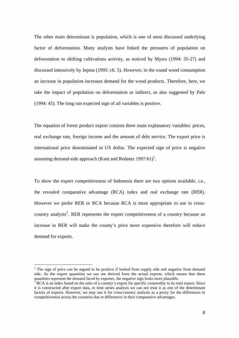
The other main determinant is population, which is one of most discussed underlying

factor of deforestation. Many analysts have linked the pressures of population on

deforestation to shifting cultivations activity, as noticed by Myers (1994: 35-27) and

discussed intensively by Jepma (1995: ch. 5). However, in the round wood consumption

an increase in population increases demand for the wood products. Therefore, here, we

take the impact of population on deforestation as indirect, as also suggested by Palo

(1994: 45). The long run expected sign of all variables is positive.

The equation of forest product export consists three main explanatory variables: prices,

real exchange rate, foreign income and the amount of debt service. The export price is

international price denominated in US dollar. The expected sign of price is negative

assuming demand-side approach (Kant and Redantz 1997:61)1.

To show the export competitiveness of Indonesia there are two options available, i.e.,

the revealed comparative advantage (RCA) index and real exchange rate (RER).

However we prefer RER or RCA because RCA is more appropriate to use in cross-

country analysis2. RER represents the export competitiveness of a country because an

increase in RER will make the county’s price more expensive therefore will reduce

demand for exports.

1 The sign of price can be argued to be positive if looked from supply side and negative from demand side. As the export quantities we use are derived form the actual exports, which means that these quantities represent the demand faced by exporter, the negative sign looks more plausible. 2 RCA is an index based on the ratio of a country’s export for specific commodity to its total export. Since it is constructed after export data, in time series analysis we can not treat it as one of the determinant factors of exports. However, we may use it for cross-country analysis as a proxy for the differences in competitiveness across the countries due to differences in their comparative advantages.

8

Foreign income or importer’s income in particular will determine the demand for a

partner’s country exports. Here, we choose the Japanese income as a proxy of the

importer because of its dominant share in export market of forest product from

Indonesia3. The impact of Japanese GDP on Indonesia’s exports for forest products

should be positive.

Export of forest products contributes the largest foreign reserve flows in Indonesia’s

non-oil sectors. Therefore it is suspected that the government had promoted the forest

product export in order to obtain certain amount of foreign reserve to service the large

amount of Indonesian debt. As a result, we expect the positive effect of debt services on

forest product exports.

In cereal cropland equation, the key explanatory variables determining change in food

cropland are variation in the cereal outputs, change in population and change in income

per capita. Variation in the output of cereals is represented by its production index. The

need to feed large population in developing countries is as the main reason for their

governments to pursue agriculture expansion towards food self-sufficiency (Capistrano

1994: 76). Therefore an increase in population increases demand for cereal lands.

Income per capita affects the demand for cereal cropland indirectly based on the fact

that a better income encourages people to work in non-agriculture sector. As a result, an

increase in income per capita will be positively associated with less demand on cereal

cropland. In sum, the sign of coefficients of the first two variables should be positive

while the last should positive.

3 The set of data obtained from FAO statistics home page : http://apps.fao.org/faostat/forestry/

9

For oil palm sub-sector, the main variables affecting change in oil palm cropland are

external debt, world price, real exchange rate, income per capita and population. Crude

palm oil production has played an important role as a valuable source of foreign reserve

when exported and as the raw inputs of the main cooking oil consumed in Indonesia

(Cason 2002: 223). The world price, real exchange rate and the amount of external debt

will express the driving factor of exports while population serves as the variable

affecting domestic consumption of palm oil.

The coefficients of external debt, real exchange rate and population are expected to be

positive. Meanwhile the international price coefficient is more likely to be negative by

assuming international demand driving the production so an increase in world price

reduces the demand for cropland area following the decline in output demanded.

The last equation is for natural rubber sub-sector. According to FAOSTAT data, most of

Indonesia’s rubber outputs are for international supply4. Therefore variation in outputs,

change in international prices and total external debt and economic growth are meant to

be the key variables explaining the growing land area needed for rubber plantations. The

expected signs for all coefficients are positive, except for international price due to

demand driven assumption.

4 During the period of examination (1961-2000), the average ratio of the amount of rubber exported to the total production is about 93%.

10

Data and its Sources

Most data in agriculture and forestry are from FAO statistics database, available on line

at www.apps.fao.org. This database has enabled us to create a data series from 1961 to

2000. The macroeconomic data are obtained from International Financial Statistics of

the IMF (CD-ROM August 2004) and The World Development Indicators of the World

Bank (CD-ROM July 2004). Table 2 exhibits the definition and sources of the data used

in this study in detail by sector.

Table 2 Variable Descriptions

SECTOR VARIABLES DESCRIPTION UNITS SOURCE Forest DEF Annual forest cover decline ‘000 hectares FAOSTAT, WB RWCON Annual industrial roundwood

consumption million M3 FAOSTAT

FOREXP Annual forest product exports million M3 FAOSTAT Agriculture DCERL Annual change in cereal harvested area ‘000 hectares FAOSTAT DPALML Annual change in oil palm harvested area ‘000 hectares FAOSTAT DRUBL Annual change in rubber harvested area ‘000 hectares FAOSTAT DCERIND Annual change in the cereal production

index (1999-2001=100) FAOSTAT

DCPOP Annual change in production of crude palm oil (CPO)

‘000 metric tones FAOSTAT

DRUBP Annual change in production of rubber ‘000 metric tones FAOSTAT International Prices

EXPR Forest product export prices US $ per M3 FAOSTAT

DICPOPR Annual change in the international CPO price indices (Malaysia, N.W. Europe, 2000 = 100)

IMF

DIRUBRR Annual change in the International rubber price indices (2000=100)

IMF

Macroeconomic

TGDP total GDP (2000 prices) Million Rupiah IMF (processed)

DGDPCAP Annual change in GDP per capita Million Rupiah IMF (processed) GDPGR The real growth of GDP Percent IMF (processed) EXDEBT Total External Debt Billion USD WB DEXDEBT Annual change in total external debt Billion USD RER Real Exchange Rate Rupiah per 1 USD IMF (processed) DRER Annual change in RER Rupiah per 1 USD IMF (processed) JAPGDP Total GDP of Japan (1995 prices) Billion USD IMF(processed) Demography TPOP Total Population Millions WB DPOP Annual change in total population Millions WB POPGR Annual population growth Percent WB

11

Estimation Models and Methods

The recursive system in this model is estimated using two-stage methods. In the first

stage, all the five endogenous variables in second-level systems are regressed to their

respective explanatory variables using ordinary least squares (OLS) to obtain these

estimated values. In the second-stage, these estimated values now act as the instrument

variables to be used in the least squares regression of the final endogenous variable. By

doing this two-stage method, the estimation of the recursive model using least squares

will be consistent and efficient, based on the important assumptions that cov(Y1, U1)=0

and cov(U1, Ui)=0 where i=2,3,4,5, and 6 (Greene 2003: 397). The complete equations

are expressed in the estimation models as follow.

The First-Stage Estimation Models:

(1) {1- }RWCONt =a1 + a2,3,4,5 TGDPt + a6 TPOPt + u2 2

1

( )a L3

0

( )b L

(2) FOREXPt = b1 + b2 EXPRt + b3 JAPGDPt + b4 EDEBTt + b5 RERt + + u3 9

6

( )b L

(3) DCERLt = c1 + c2 DCERINDt + c3 DGDPCAPt + c4 POPGR + u4

(4) DPALMLt = d1+ d2 DCPOPt + d3 DICPOPRt + d4 DEXDEBTt + d5 DRERt + d6

GDPCAPt

+d7 DEXDEBTt-1 + u5

(5) DRUBLt = e1 + e2 DRUBPt + e3 DIRUBPRt + e4 GDPGR + e5 EEXDEBTt +

e6 DRUBPt + + u6 8

7

( )b L

The Second-stage estimation models:

(1) DEFt = a1 RWCON_HATt + a2 FOREXP_HATt + a3 DCERL_HATt

+ a4 DPALML_HATt + DRUBL_HATt + u1

In the first-stage estimations, there is a high probability of error terms being correlated

as common problems in time series analysis. In the presence of serial correlation, the

12

OLS estimates are unbiased and consistent, but inefficient (Gujarati 1995: 410). As a

result, inference based on OLS estimates might be misleading. To overcome this

problem, lag operators for dependent and (or) explanatory variables will be introduced

to capture dynamic patterns of the model. Then, the LM Breusch-Godfrey tests for

autocorrelations on residuals will be conducted to check the presence of autocorrelation

in the equations (Greene 2003: 271). Due to the use of a small sample in our case, the

robustness of the standard errors to the presence of heteroskedasticity then is checked

using the white tests (Wooldridge 2001: 399)5. All estimations and tests are conducted

with help of the econometric package Eviews ver.4.1.

Results and Discussion

The results of the six equations are presented next in terms of the estimated coefficients,

t-value and the long-run multiplier when necessary. The significance of impact

multiplier is tested using normal procedure of individual tests when for long-run

multiplier using the wald restriction tests. The results of serial correlation tests and

heteroskedasticity tests are given in Appendix.

Roundwood Consumption

The results of the roundwood consumption equation are as in Table 3. The estimated

impact multiplier of national income appears to have a correct sign but it is not

statistically different from zero at the critical value of 5 percent.

5 Although the major problem in time series regression models is the presence of autocorrelation, heteroskedasticity might also occur in time series analysis, especially in the small sample case.

13

In the long run, national income also has no effect on roundwood consumption6. The

insignificancy of national income to affect domestic round-wood consumption may be

explained by the fact that logging concession holders, who produce roundwood, and the

investors in timber industry being at the same hands. As a result, the consumption of

roundwood is likely to be vertically determined by investment in timber industry instead

of the effect of aggregate income level.

The estimated coefficients of the impact and long-run multipliers of the population are

positive and statistically significant7. Population has a cumulative effect on roundwood

consumption, which is relatively small in the short-run, that is, 0.139, but which

becomes substantially larger in the long-run, that is, 2.152. This indicates that growing

population causes a persistent and increasing consumption of roundwood.

Table 3 Regression results of roundwood consumption equation

Endogenous variable = RWCONt

Variable Coefficient t-value LR-multiplier

INTERCEPT** -13.70812 -2.034687

TGDPt 0.008341 0.735743

TPOPt** 0.139272 2.179387 2.1519

3

1

( )b L TGDP -0.020871

1 - 2

1

( )a L 0.06472

R2 = 0.98; ** : significant at 5% (one tail t test).

6 Under the null hypothesis of no long run effect of the national income variable, the wald test statistic is 4.1052 where the relevant critical value of the F distribution at 5% significance is 4.185. Here our observed TS is smaller than CV so we fail to reject the null hypothesis and conclude that national income have no long run effect on roundwood consumption 7 Since population has no lagged variables, the individual test using t- distribution is sufficient to test the significance of both short and long-run multipliers, which are statistically significant at 5 percent.

14

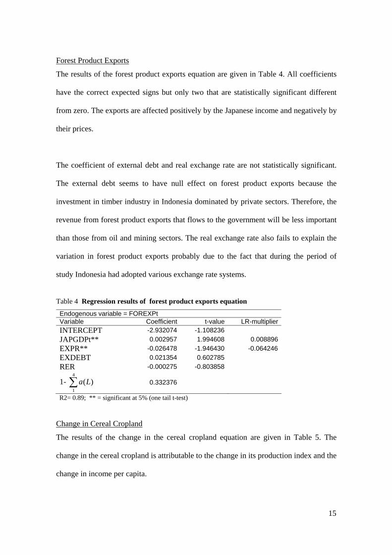
Forest Product Exports

The results of the forest product exports equation are given in Table 4. All coefficients

have the correct expected signs but only two that are statistically significant different

from zero. The exports are affected positively by the Japanese income and negatively by

their prices.

The coefficient of external debt and real exchange rate are not statistically significant.

The external debt seems to have null effect on forest product exports because the

investment in timber industry in Indonesia dominated by private sectors. Therefore, the

revenue from forest product exports that flows to the government will be less important

than those from oil and mining sectors. The real exchange rate also fails to explain the

variation in forest product exports probably due to the fact that during the period of

study Indonesia had adopted various exchange rate systems.

Table 4 Regression results of forest product exports equation

Endogenous variable = FOREXPt Variable Coefficient t-value LR-multiplier INTERCEPT -2.932074 -1.108236 JAPGDPt** 0.002957 1.994608 0.008896

EXPR** -0.026478 -1.946430 -0.064246

EXDEBT 0.021354 0.602785 RER -0.000275 -0.803858

1- 4

1

( )a L 0.332376

R2= 0.89; ** = significant at 5% (one tail t-test)

Change in Cereal Cropland

The results of the change in the cereal cropland equation are given in Table 5. The

change in the cereal cropland is attributable to the change in its production index and the

change in income per capita.

15

The growth rate in cereal land use is in line with the growth rate in production. This

may indicate that efficiency level in terms of land uses for cereal production had

relatively unchanged during the period of examination. At the same time, growth in

income per capita had negative impact on growth in the cereal cropland. This may

suggests that a better income per capita discourage the expansion of cereal cropland.

However population growth is not an important factor explaining the land change use

for cereal crops. This situation may exhibit that the growth in population does not

necessarily induce the cereal cropland expansions because less young people are willing

to work in subsistence agriculture producing staple foods like paddy and maize. High

input prices and low output prices are several factors behind the unattractiveness of the

cereal crops sub-sector.

Table 5 Regression results of the change in cereal cropland equation

Endogenous variable = DCERL

Variable Coefficient t-valueIntercept -187.3610 -0.438682DCERINDt*** 235.8968 7.523468DGDPCAPt** -788.9943 -1.724892POPGRt -0.303630 -0.111767

R2= 0.62; **: significant at 5%; ***: at 1% (one tail t-test)

Change in Oil-Palm Cropland

The results of the change in the oil-palm cropland equation are given in Table 6. Five

variables is statistically significant in explaining the variation in land use change for

palm oil sub-sector. The expansion in the cropland is along with the expansion in

production but not with its international output prices.

16

The factor that much matters in context of international trade in this case is the real

exchange rate. The Rupiah devaluation policy or depreciation made Indonesia’s

products cheaper internationally. As a result, the demand for palm-oil increases, which

in turn inducing land expansion for palm-oil plantations.

The effect of external debt is lagged one period to influence the change in oil-palm

cropland. This may suggest that substantial investment in oil-palm sub-sector is come

from overseas, which then increases the international liabilities in the following period.

The change in income per capita contributed positively to the change in oil-palm

cropland. This indicates that higher income increases demand for CPO as the raw

materials for most cooking oil in Indonesia.

Table 6 Regresssion results of change in oil-palm cropland equation

Endogenous variable = DPALMLt Variable Coefficient t-valueIntercept -13.81905 -1.657791DCPOPt*** 0.018124 2.085043DICPOPRt** -0.224319 -2.079911DEXDEBTt 0.191859 0.152381DRERt*** 0.048829 4.080188DGDPCAPt*** 226.2067 3.013606DEXDEBTt-1** 2.858095 2.615255


Note: Newey-West HAC Standard errors (lag truncation of 3) is applied here since the white heteroskedasticity indicate the presence of hetreoskedasticity in the equation

Change in Rubber Cropland

The results of the change in the rubber cropland equation are given in Table 7. The

variation in the change in the rubber cropland equation is explained by the change its

international prices and the rate growth of GDP.

17

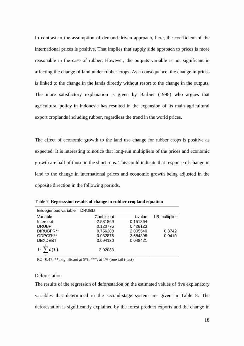
In contrast to the assumption of demand-driven approach, here, the coefficient of the

international prices is positive. That implies that supply side approach to prices is more

reasonable in the case of rubber. However, the outputs variable is not significant in

affecting the change of land under rubber crops. As a consequence, the change in prices

is linked to the change in the lands directly without resort to the change in the outputs.

The more satisfactory explanation is given by Barbier (1998) who argues that

agricultural policy in Indonesia has resulted in the expansion of its main agricultural

export croplands including rubber, regardless the trend in the world prices.

The effect of economic growth to the land use change for rubber crops is positive as

expected. It is interesting to notice that long-run multipliers of the prices and economic

growth are half of those in the short runs. This could indicate that response of change in

land to the change in international prices and economic growth being adjusted in the

opposite direction in the following periods.

Table 7 Regresssion results of change in rubber cropland equation

Endogenous variable = DRUBLt

Variable Coefficient t-value LR multiplier Intercept -2.581869 -0.151864 DRUBP 0.120776 0.428123 DIRUBPR** 0.756208 2.005540 0.3742 GDPGR*** 0.082875 2.684398 0.0410 DEXDEBT 0.094130 0.048421

1- 2

1

( )a L 2.02083


Deforestation

The results of the regression of deforestation on the estimated values of five explanatory

variables that determined in the second-stage system are given in Table 8. The

deforestation is significantly explained by the forest product exports and the change in

18

cereal cropland at 5 percent of significance. The other two variables are not statistically

significant in affecting the deforestation.

The coefficient of forest product exports suggests that an annual increase of one million

cubic metres of quantity exported contributes to the annual forest cover loss of 24

thousand hectares. The coefficient of change in cereal cropland is 0.3, which is far away

from one-to-one relationship between the amount of forest decline and the amount

increase in the land under cereal productions.

In general, this model gives a poor estimates as shown by the extremely low of the

goodness of fit (R2) in which only fourteen percent variation in deforestation may be

attributed to the variations in its explanatory variables. The main problem with the

deforestation model is due to data reliability, which is in this study is derived form

FAOSTAT. The technique of data collection by FAO is through the answer of

questionnaire distributed by FAO to the reporting countries. The participant’s

governments in fill the questionnaires may have incentives to underrate the extent of

deforestation to avoid the reputation damage.

Table 8 Regression results of the deforestation equation

Endogenous variable = DEFt

Variable Coefficient t-value

RWCON_HAT -1.633690 -0.162652

FOREXP_HAT** 24.91054 1.873048

DCERL_HAT** 0.300320 1.920256

DPALML_HAT 3.476668 1.030126

DRUBL_HAT 0.345862 0.132951

R2= 0.14 ; **: significant at 5% (one-tail t test)

19

Impact of underlying causes on deforestation

Based on the two variables that significantly determining deforestation, only income per

capita is identified as one of factors extensively discussed as underlying causes of

deforestation. However, the effect is to ease the rate of deforestation because an increase

in income per-capita is suggested to reduce the land expansion for cereal crops. This

conclusion is along with the observation Lombardini (1994) in case study of

deforestation in Thailand as it is found that the income per capita negatively affected the

forest cover.

The others indirect causes are come form international market pressures on forest

products in forms of the importer’s income and the international prices. The Japanese

income is meant to be indirect cases of deforestation in Indonesia through the forest

product exports equation.

Conclusions

This study has attempted to develop an economic model for deforestation in Indonesia

by using time series data form 1961 to 2000. The results of the model are definitely

subject to the limitation of data. Nevertheless, it can be shown that the exportation of

forest products from Indonesia to meet the growing demand of international community

has resulted in the substantial decline in forest cover. Another pressure comes form the

need of land conversions for cereal productions. However, the impact of the change in

land uses under cereal crops appears to be much lower than the expectation of one to

one relationship. The most frequently discussed underlying variables have been

discussed, but the low goodness of fit of our deforestation model prevents us to draw

some policy recommendation based on this study.

20

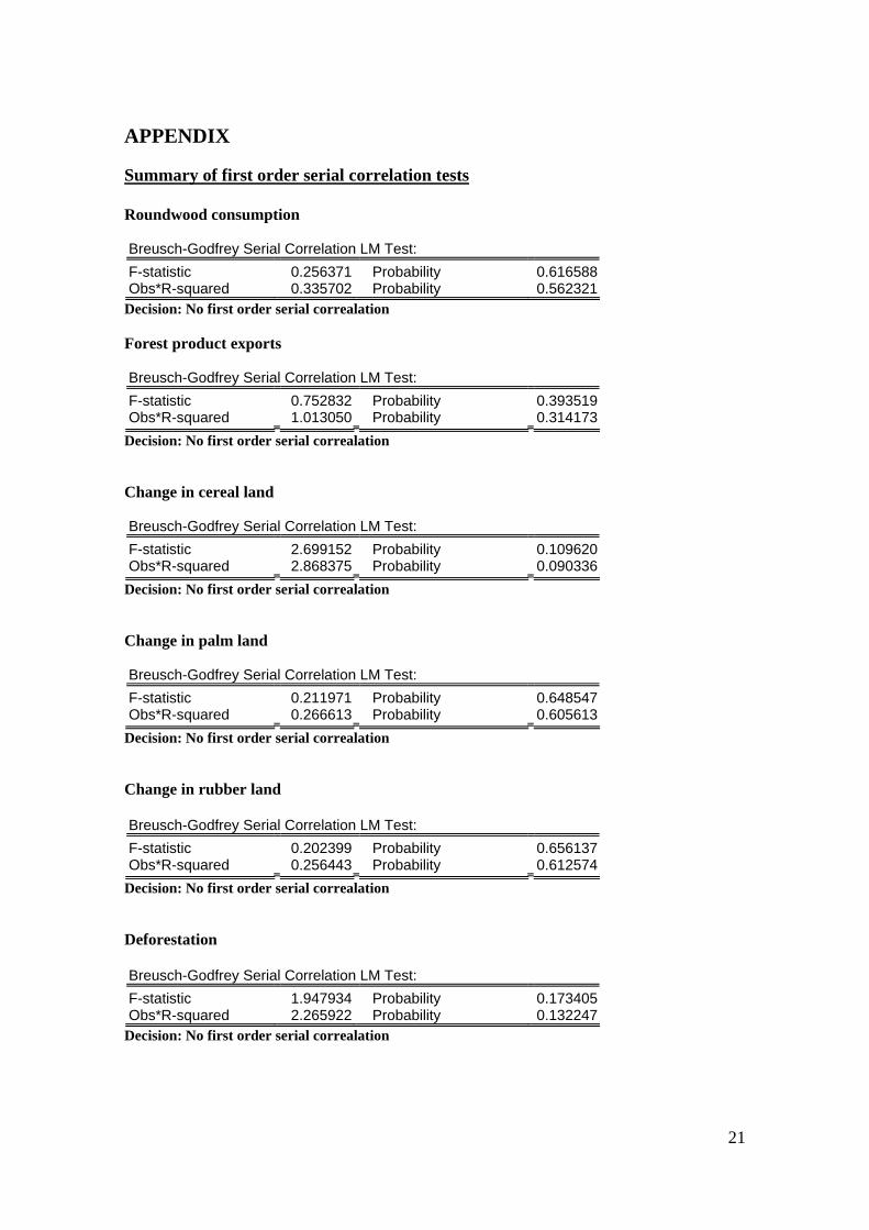
APPENDIX

Summary of first order serial correlation tests Roundwood consumption Breusch-Godfrey Serial Correlation LM Test:

F-statistic 0.256371 Probability 0.616588Obs*R-squared 0.335702 Probability 0.562321

Decision: No first order serial correalation Forest product exports Breusch-Godfrey Serial Correlation LM Test:


Decision: No first order serial correalation Change in cereal land Breusch-Godfrey Serial Correlation LM Test:


Decision: No first order serial correalation Change in palm land Breusch-Godfrey Serial Correlation LM Test:


Decision: No first order serial correalation Change in rubber land Breusch-Godfrey Serial Correlation LM Test:


Decision: No first order serial correalation Deforestation Breusch-Godfrey Serial Correlation LM Test:


Decision: No first order serial correalation

21

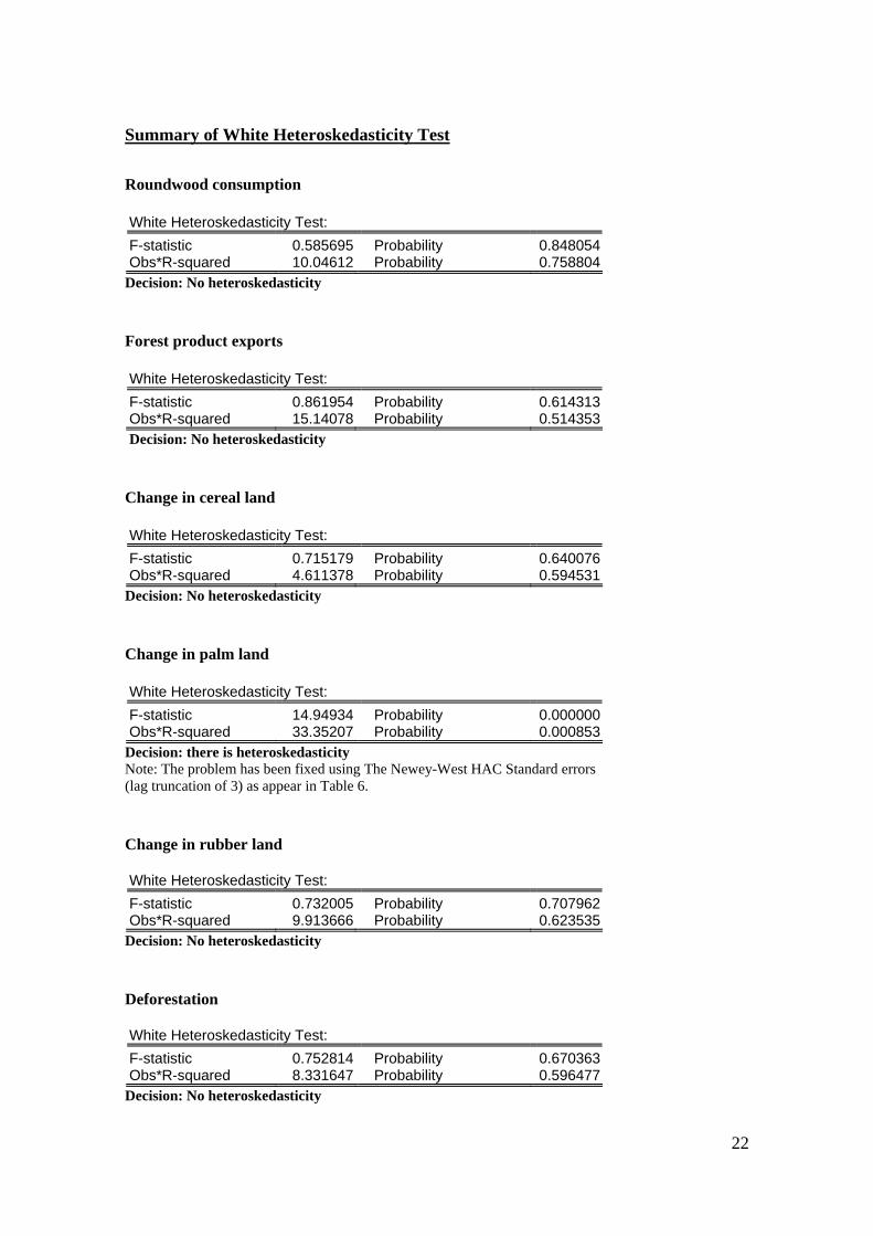
Summary of White Heteroskedasticity Test

Roundwood consumption White Heteroskedasticity Test:


Decision: No heteroskedasticity Forest product exports White Heteroskedasticity Test:

F-statistic 0.861954 Probability 0.614313Obs*R-squared 15.14078 Probability 0.514353 Decision: No heteroskedasticity Change in cereal land White Heteroskedasticity Test:


Decision: No heteroskedasticity Change in palm land White Heteroskedasticity Test:


Decision: there is heteroskedasticity Note: The problem has been fixed using The Newey-West HAC Standard errors (lag truncation of 3) as appear in Table 6. Change in rubber land White Heteroskedasticity Test:


Decision: No heteroskedasticity Deforestation White Heteroskedasticity Test:


Decision: No heteroskedasticity

22

References Angelsen, A. and Kaimowitz, D., 1999. Rethinking Causes of the Causes of

Deforestation: Lessons from Economic Models, The World Bank Research Observer 14 (1): 73-98.

Aswicahyono, H., 2004. Competitiveness and Efficiency of the Forest Product Industry

in Indonesia, CSIS Working Paper Series WPE 075 (February), Centre for Strategic and International Studies (CSIS), Jakarta.

Barbier, E., 1998. ‘Cash crops, food crops, and sustainability: the case of Indonesia’ in

Barbier, E. (ed), The Economics of Environment and Development, Edward Elgar Publishing, UK.

Barr, C., 2001. Banking on Sustainability: Structural Adjustment and Forestry Reform

in Post-Suharto Indonesia, WWF/CIFOR, Bogor. Capistrano, A. D., 1994. ‘Tropical Forest Depletion and the Changing Macroeconomy,

1967 – 85’ in Brown, K. and Pearce, D.W. (eds), The Causes of Tropical Deforestation, UCL Press, London.

Casson, A, 2002. ‘The Political Economy of Indonesia’s Oil Palm Subsector, in Colfer,

C.J.P. and Resosudarmo, I.A.P (eds), Which way foward ? People, Forests, and Policymaking in Indonesia, RFF. Washington, D.C.

Christanty, L., and Atje, R., 2004. Policy and Regulatory Developments in the Forestry

Sectors Since 1967, CSIS Working Paper Series WPE 077, Centre for Strategic and International Studies (CSIS), Jakarta.

Colfer, C.J.P., and Resosudarmo, I.A.P. (eds), 2000. Which way foward ? People,

Forests, and Policymaking in Indonesia, RFF. Washington, D.C. Contreras-Hermosilla, A., 2000. The Underlying Causes of Forest Decline, CIFOR,

Bogor, Indonesia Erwidodo and Astana, S., 2004. Agricultural-Forestry Linkages: Development of

Timber and Tree Crop Plantations Towards Sustainable Natural Forests, CSIS Working Paper Series WPE 078, Centre for Strategic and International Studies (CSIS), Jakarta.

FAO, 2001. Forest Resource Assessment 2000, FAO Forestry Paper 140, Rome.

Available at: www.fao.org/forestry/site/fra/en FWI/GFW, 2002. The State of Forest: Indonesia, Bogor, Indonesia: Forest Watch

Indonesia, and Washington DC: Global Forest Watch. Geist, H.J. and Lambin E.F. 2002. Proximate Causes and Underlying Driving Forces of

Tropical Deforestation, BioScience 52 (2) : 143 – 150.

23

24

Greene, W.H. 2003. Econometric Analysis, Upper Saddle River, New Jersey. Gujarati, D. 1995. Basic Econometrics, McGraw-Hill. Holmes, D. A., 2002. Indonesia: Where Have All the Forests Gone?, Environment and

Social Development Unit, East Asia and Pacific Region Discussion Paper, The World Bank.

Jepma, J.P., 1995. Tropical Deforestation: A Socio-Economic Approach, Earthscan, The

United Kingdom. Kant, S and Redantz, A., 1997. An Econometric Model of Tropical Deforsetation,

Journal of Forests Economics 3 (1): 51-86. Lombardini, C. 1994. ‘Deforestation in Thailand’ in Brown, K. and Pearce, D.W. (eds),

The Causes of Tropical Deforestation, UCL Press, London. Myers, N., 1994. ‘Tropical Deforestation: Rates and Patterns’ in Brown, K. and Pearce,

D.W. (eds), The Causes of Tropical Deforestation, UCL Press, London. Nasendi, B. D., 2000. ‘Deforestation and Forest Policies in Indonesia’ in Palo, M. and

Vanhanen, H. (eds) World Forests from Deforestation to Transition?, Kluwer Academic Publisher, The Netherlands.

Purnama, B. M., 2003. Sustainable Forest Management as a Basis for Improving the

Role of The Forestry Sector, Department of Forestry, Indonesia. Rowe, B. and Sharma, N.P., 1992. ‘Deforestation: Problems, Causes, and Concerns’, in

Sharma, N.P. (ed), Managing the World’s Forests, Kendal/Hunt Publishing, Iowa.

Sunderlin, W.D. and Resosudarmo, I.A.P., 1996, Rates and Causes of Deforestation in

Indonesia: Towards a Resolution of the Ambiguities, CIFOR, Bogor, Indonesia.

Wooldridge, J.M. 2001, Introductory Econometrics: A Modern Approach, South-

Western College Publishing. World Bank, 2000. Indonesia: The Challenges of World Bank Involvement in Forests,

Evaluation Country Case Study Series, Washington D.C.

Documents

An Econometric Model for Deforestation in Indonesia