An Econometric Model of Location and Pricing in

the Gasoline Market

Tat Y. Chan ∗

V. Padmanabhan †

P.B. Seetharaman ‡

July 26, 2006

∗Assistant Professor of Marketing, John M. Olin School of Business, Washington University, St. Louis, e-mail:chan@wustl.edu.

†INSEAD Chaired Professor of Marketing, INSEAD, Singapore, e-mail: paddy.padmanabhan@insead.edu.‡Address for correspondence: Associate Professor of Management, Jesse H. Jones Graduate School of Man-

agement, Rice University, MS 531, 6100 S Main, Houston, TX 77005. Email address: seethu@rice.edu. Ph:713-348-6342. Fax: 713-348-6296. Authors are listed in alphabetical order. We thank Yuanfang Lin for settingup the data in usable form for our empirical analyses. We thank Prof. Glenn MacDonald and Prof. Mark Daskinfor their valuable guidance and comments during the preliminary stages of this project. We appreciate the manyinsightful comments by participants at the Summer Institute of Competitive Strategy, Berkeley, CA (July 2003),the Marketing Camp at the Kellogg School of Management, Northwestern University, Chicago, IL (Sep 2003),the seminars at Jesse H. Jones School of Management, Rice University (Nov 2003), INSEAD (Nov 2003), Whar-ton School, University of Pennsylvania (Jan 2004), Indian Institute of Management, Ahmedabad, India (August2004), National University of Singapore (August 2004), and Korea University Business School (KUBS), Seoul(May 2006). Last, but not the least, we gratefully acknowledge the assistance of Prof. Ivan Png, Mrs. Priti Devi,Mr. Albert Tan, Mr. Low Siew Thiam, Mr. Henry Wee and Mr. Eng Kah Joo.

1

An Econometric Model of Location and Pricing in the Gasoline Market

Abstract

The authors propose a econometric model of both the geographic locations of gasolineretailers in Singapore, as well as price competition between these retailers conditional on theirgeographic locations. Although market demand for gasoline are not observed, the authorsare able to infer the effects of such demand from stations’ location and pricing decisionsusing available data on local market-level demographics. Using the proposed location model,that is based on the assumption of social welfare maximization by a policy planner, theauthors find that local potential gasoline demand depends positively on the following localdemographic characteristics of the neighborhood: population, median income, number ofcars, proximity to airport, downtown and highways. Using the proposed pricing model,that is based on the assumption of Bertrand competition between retail chains, the authorsfind retail margins for gasoline to be about 21%. The authors also find that consumers arewilling to travel up to a mile for a price saving of 3 cents per liter. Using the estimates ofthe proposed econometric model, the authors answer policy questions pertaining to a recentmerger between two firms in the industry. Answering these questions has important policyimplications for both gasoline firms and policy makers in Singapore.

Keywords: Location Modeling, Networks, Discrete Locations, Price Competition, GasolineMarkets, P-Median Problems, Empirical Industrial Organization, Econometric Models.

2

Location is repeatedly stressed in the business press as one, if not the only, requirement

for success in retailing. It is also recognized in the academic literature as being an important

determinant of retail competition and performance. In fact, some of the earliest work on retail

competition (e.g., Hotelling 1929, D’Aspremont, Gabszewicz and Thisse 1979) were based on

models of spatial heterogeneity given the location decisions of retail firms. This paper attempts

to understand the phenomenon of retail performance by developing an econometric model of

location and price decisions. The simultaneous consideration of both location and marketing-

mix interactions allows us to address a broader set of questions related to public policy as well as

to provide a more comprehensive answer to questions of firm conduct and market performance.

For example, we can now address questions such as

• What are the important factors contributing to the potential demand at a location?

• How important is a retailer’s geographic location when consumers choose among alternative

retailers? What are the trade-offs involved for a retailer between facing large potential

demand at a location versus being in close proximity to competitors at the location?

• What will be the impact of a merger between two retail chains on prices and profits in the

retail industry?

The context for this paper is the gasoline market in Singapore. Using a primary dataset

- representing a census of all gasoline stations in Singapore -that tracks geographic locations,

gasoline prices and various station characteristics across 226 gasoline stations, as well as the

demographic characteristics of the stations’ local neighborhoods, we undertake the estimation

of an econometric model of location and pricing decisions of gasoline stations.

The location model is built on the premise (which is consistent with institutional realities

in Singapore, as discussed in the data description section) that the Singapore government de-

termines where to locate gasoline stations in the city. The government, being a social welfare

planner, is assumed to minimize aggregate travel costs incurred by consumers in their efforts to

buy gasoline in Singapore. This leads to a decision model that is called a P-Median problem.

We use a minimum-distance method to estimate such a location model, that enables us to infer

3

the geographic distribution of potential gasoline demand across local markets in Singapore, and

the dependence of such demand on local demographic characteristics.

We then propose a pricing model for gasoline stations, conditional on their locations, based

on the premise of Bertrand competition between retail chains. The pricing model requires local

firm-level demand - which is a function of the potential demand for gasoline at various locations,

prices and gasoline characteristics - as inputs. Since gasoline demand is unobserved in the data,

we use equilibrium conditions of demand and supply to obtain an estimable model of pricing.

Estimating the pricing model allows us to infer both the cost and demand functions. Using the

estimates of the parameters of the location model and pricing model, we answer policy questions

pertaining to the relative profitability of various retail chains, as well as the consequences of a

merger between two retail chains on prices and profits of firms in the industry.

From estimating our proposed location model, we find that local potential gasoline demand

depends positively on the following local demographic characteristics of the neighborhood: pop-

ulation, median income, number of cars, proximity to airport, downtown and highways. Using

the estimated potential gasoline demand at each local neighborhood in Singapore as an input,

we then estimate our proposed pricing model using empirical data on actual prices of gasoline

at various stations. We find retail margins for gasoline to be about 21%, and that market share

for a gasoline station is negatively influenced by the price of gasoline and travel cost. We find

that consumers are willing to travel up to a mile for a price saving of 3 cents per liter (which

translates to a saving of about $1.3 on a 40-liter tank of gasoline).

Relationship to the Literature

The primary contribution of this paper is in developing an econometric model of location and

pricing decisions in the gasoline market. We position it in the context of previous research on

gasoline markets, as well as previous research on retail competition models.

Gasoline Markets

Shepard (1991) and Iyer and Seetharaman (2003) estimate pricing models for gasoline stations

that have local monopoly power. Their models are not applicable for competitive markets, as in

this paper. Slade (1992) estimates a competitive pricing model using time-series data on demand

4

and prices at 13 gasoline stations in the Greater Vancouver area. In focusing only on a limited

number of firms in the same geographic neighborhood, the model ignores the role of location on

competition. Png and Reitman (1994) and Iyer and Seetharaman (2005) address the puzzle of

why retailers in the same geographic space adopt very similar strategies in certain instances and

very different strategies in other cases assuming retail location decisions as exogenous. Pinkse,

Slade and Brett (2002) estimate a competitive pricing model that accommodates the effects of

spatial locations of firms. However, all of these studies take a reduced-form approach to modeling

the effects of location on price competition between firms. In contrast, we estimate an economic-

theoretic model of pricing behavior in this study, as in Manuszak (1999). Further, none of the

above studies attempts to explain location decisions of firms. We believe that our paper is the

first effort at modeling location decisions in gasoline markets. The institutional reality that the

Singapore government serves as a social planner in determining locations of gasoline stations

makes our location model both realistic and mathematically tractable.

Retail Competition Models

Models of entry and exit decisions of firms, based on free entry of firms (as opposed to a social

planner determining the optimal locations), have been recently proposed by Mazzeo (2002), who

models the local market entry decisions of hotels, and by Seim (2004), who models local market

entry decisions of video retailers (see Dube, Sudhir et al. 2005 for a review of the literature

on entry models). Our modeling approach differs from theirs in that we model the location

decisions – as opposed to the entry and exit decisions – of a fixed number of gasoline stations

in geographic space, using the observed geographic distribution of geo-demographic variables in

that space.

A rich literature exists in marketing that casts firms and consumers on a common perceptual

map in order to analyze optimal marketing decisions of firms (Hauser and Shugan 1983, Hauser

1988, Moorthy 1988, Choi, Desarbo and Harker 1990 etc.). Marketing models of this type

recognize that brands occupy different positions - in terms of not only their objective attributes,

but also consumers’ subjective evaluations of these attributes - in the perceptual map, while

consumers have different ideal points (i.e., most preferred combinations of attributes) on the

same perceptual map. Our location model can be viewed in light of this literature as one where

5

consumers’ ideal points correspond to their place of residence or work, while brand positions

correspond to the geographic locations of stores. Consumers’ ideal points are inferred as a

function of geographic characteristics in our case, unlike in the perceptual map literature where

subjectively perceived brand positions, as well as consumers’ ideal points for attributes, are

measured using marketing research techniques. It is useful to note that location is a horizontal

attribute (i.e., different consumers would disagree on what is the best location for a firm, based

on where their ideal points reside), as opposed to attributes such as price and quality that are

vertical attributes (i.e., all consumers would agree that lower price is preferable to higher price,

higher quality is preferable to lower quality etc.).

Recently, Thomadsen (2003) has developed a retail price competition model based on the

assumption of Bertrand price competition between fast-food retail chains. This model uses a

multinomial logit model of demand as an input to the pricing equations. Demand for retailers are

parameterized as a function of observed geographic characteristics, prices and travel distances of

consumers to stores. Both demand- and supply-side parameters are inferred solely from observed

prices, since demand for various retailers are not observed in the data. Since we also do not

observe demand for gasoline retailers in our data, we adopt the Thomadsen (2003) approach to

model price competition between retailers. However, unlike Thomadsen (2003), who relies on the

pricing model only, we use a location model that exploits the observed geographic distribution

of gasoline stations across local markets to infer the potential gasoline demand at each local

market.

The remainder of the paper is organized as follows. In Section 3 we develop empirical models

to estimate location and pricing decisions of gasoline stations in Singapore, along with estimation

techniques to estimate model parameters. In Section 4 we describe our data. Section 5 presents

the empirical results of our analyses. In Section 6, we discuss the policy implications of our

results. Concluding remarks are made in Section 7.

Model of Location and Pricing Decisions of Gasoline Stations inSingapore

We present this section in two parts. First, we develop a model of gasoline stations’ locational

choices by the government, making explicit the parametric specification of the location model,

6

and discussing estimation details. Second, we develop a model of gasoline pricing decisions

conditional on the observed locational choices, presenting a specific parameterization of the

pricing model, and setting up the estimation procedure.

Location Model

It is useful to note the following two features of the gasoline market in Singapore (that make it

different from the gasoline market in the US):

1. Gasoline stations can only be built on specified plots determined by the government. Land

is offered on a public tender in an open-bid system, and any company can bid. In other

words, bidding decisions of oil companies only determine who owns each location, and not

where the locations themselves ought to be.

2. Price competition among gasoline stations in Singapore is a relatively recent phenomenon.

Prior to this, gasoline prices were determined on the basis of a multi-lateral agreement

between the Singapore government and gasoline retailers. Therefore, prices were assumed

to be equal by the Singapore government while determining optimal locations for gasoline

stations.

On account of the above two features of the Singapore gasoline market, we make the following

assumptions for our location model.

1. In empirically explaining observed locations of gasoline stations in Singapore, we assume

that the Singapore government is the decision-maker.

2. Since gasoline prices are constant across gasoline stations, they do not play a role in the

location model.

3. The government picks geographic locations for the P gasoline stations so as to minimize

the total expected travelling costs of all consumers in Singapore who constitute the total

potential demand for gasoline.

4. The supply capacity of each gasoline station exceeds its potential demand, i.e., an under-

capacity problem does not exist.

7

We acknowledge that station characteristics (such as convenience store, car wash etc.) would

also affect consumers’ choices among stations, and therefore consumers’ welfare functions. How-

ever, the Singapore government cannot know, a priori, which retail chain would successfully

bid for a specific location, and the station characteristics that the chain would then choose for

that location. Therefore, it is impossible for the government to determine locations by taking

into account station characteristics at various possible locations. This underlies assumption 3

(Note: Consistent with this assumption, our estimation results from the pricing model show

that station characteristics are not as important as price or travel cost in influencing consumer

demand for gasoline stations, as will be shown later). Assumption 4 was confirmed by managers

at Exxon-Mobil, Shell and Caltex, the three major oil companies in Singapore.

By discretizing the two-dimensional map of Singapore into N equally spaced grid points, we

define the Singapore government’s problem as one of choosing P grid points, among the full set

of N available grid points, to locate gasoline stations, in order to minimize the sum of travelling

distances across all consumers who constitute potential gasoline demand. Let Yij denote a binary

outcome that takes the value 1 if consumers within grid point i choose the gasoline station in grid

point j and 0 otherwise. Based on the above discussion, the Singapore government’s objective

function can then be written down as follows (Note: Our conversations with government planners

indicate that models of this kind are routinely used in urban development):

minX

N∑i=1

N∑j=1

q(Zi;α)dijYij (1)

such that

N∑j=1

Yij = 1 (2)

N∑j=1

Xj = P (3)

Yij − Xj ≤ 0, ∀i, j (4)

Yij = 0 or 1 (5)

8

Xj = 0 or 1 (6)

where q(Zi;α) is the potential demand for gasoline at grid point i, Zi is a vector of all

relevant factors that explain potential gasoline demand at grid point i, α is the corresponding

vector of unknown parameters, dij is the geographic distance between grid points i and j, Xj

is an indicator variable that takes the value 1 if a gasoline station resides in grid point j and

0 otherwise, and Yij as a binary outcome that takes the value 1 if consumers within grid point

i choose the gasoline station in grid point j and 0 otherwise. Equation (1) is the objective

function of the Singapore government. Equation (2) embodies the constraint that consumers

within a grid point i can choose one and only one gasoline station. Equation (3) embodies the

constraint that the government is working with P stations in its locational planning decision.

Equation (4) captures the logical condition that consumers cannot choose to go to grid point

j for their gasoline purchase if no gasoline station is located at j. Equation (5) implies that

consumers at grid point i will choose either to travel to grid point j (Yij = 1) or not (Yij = 0).

Finally, equation (6) implies that a gasoline station is either set up at grid point j (Xj = 1) or

not (Xj = 0).

We specify potential gasoline demand at a grid point qi = q(Zi;α) in a log-linear manner

using the following multiplicative model (which has been extensively used to estimate the effects

of marketing mix variables on brand sales, see, for example, Van Heerde, Leeflang and Wittink

2000).

ln(qi) = α1 ln(POPi

POP0) + α2 ln(

INCi

INC0) + α3 ln(

CARi

CAR0) + α4I

AIRii + α5I

DTii + α6I

HWYii (7)

where POPi is the residential population of grid point i, INCi the median income of grid

point i, CARi the total number of owned cars in grid point i, IAIRi is an indicator variable

that takes the value 1 if grid point i is near the airport and 0 otherwise, IDTi is an indicator

variable that takes the value 1 if grid point i is in the downtown area and 0 otherwise, and

IHWYi is an indicator variable that takes the value 1 if grid point i is close to a highway and 0

otherwise. POP0, INC0, and CAR0 are explanatory variables for a reference grid point, whose

potential demand level q0 is fixed at 1 (for identification purposes). Therefore, the explanatory

9

variables for all other grid points are operationalized relative to the corresponding variables of

this reference grid point. It is useful to note that the parameters α1, α2, α3 of the multiplicative

model can directly be interpreted as the elasticities of potential gasoline demand to changes in

the relative values of the explanatory variables with respect to the reference grid point. It is

also useful to reiterate here that while potential gasoline demand at a grid point is a function

of local demographic variables, it depends on neither the prices and station characteristics of

stations that may choose to locate themselves at or near the grid point, nor on travel distances

of consumers within the grid point. This is consistent with the definition of potential market

size in the existing literature on choice models.

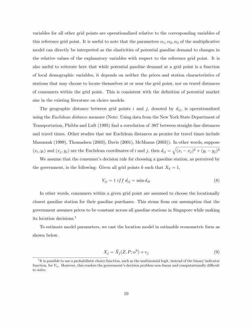
The geographic distance between grid points i and j, denoted by dij , is operationalized

using the Euclidean distance measure (Note: Using data from the New York State Department of

Transportation, Phibbs and Luft (1995) find a correlation of .987 between straight-line distances

and travel times. Other studies that use Euclidean distances as proxies for travel times include

Manuszak (1999), Thomadsen (2003), Davis (2001), McManus (2003)). In other words, suppose

(xi, yi) and (xj , yj) are the Euclidean coordinates of i and j, then dij =√

(xi − xj)2 + (yi − yj)2

We assume that the consumer’s decision rule for choosing a gasoline station, as perceived by

the government, is the following: Given all grid points k such that Xk = 1,

Yij = 1 iff dij = min dik (8)

In other words, consumers within a given grid point are assumed to choose the locationally

closest gasoline station for their gasoline purchases. This stems from our assumption that the

government assumes prices to be constant across all gasoline stations in Singapore while making

its location decisions.1

To estimate model parameters, we cast the location model in estimable econometric form as

shown below.

Xj = Xj(Z,P ;α0) + ej (9)

1It is possible to use a probabilistic choice function, such as the multinomial logit, instead of the binary indicatorfunction, for Yij . However, this renders the government’s decision problem non-linear and computationally difficultto solve.

10

where Xj is the observed location of station j, Xj(Z,P ;α0) is the predicted (based on solving

the objective of the Singapore government, as given in equation 1) location of station j, α0 is the

true value of the unknown parameter vector α (that is known to the Singapore government but

unknown to the econometrician), ej stands for measurement error (with mean zero). Minimizing

this measurement error in some manner, using an appropriate loss function, will serve as the

estimation technique to recover estimates of α. It is useful to recognize here that Xj and

Xj(Z,P ;α) are both two-dimensional variables since they represent station locations in two-

dimensional Euclidean space.

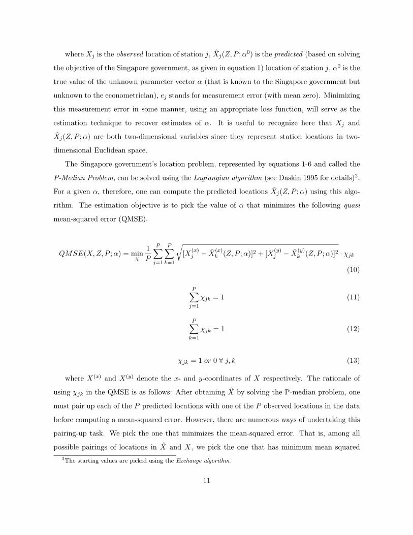
The Singapore government’s location problem, represented by equations 1-6 and called the

P-Median Problem, can be solved using the Lagrangian algorithm (see Daskin 1995 for details)2.

For a given α, therefore, one can compute the predicted locations Xj(Z,P ;α) using this algo-

rithm. The estimation objective is to pick the value of α that minimizes the following quasi

mean-squared error (QMSE).

QMSE(X, Z, P ;α) = minχ

1P

P∑j=1

P∑k=1

√[X(x)

j − X(x)k (Z,P ;α)]2 + [X(y)

j − X(y)k (Z,P ;α)]2 · χjk

(10)

P∑j=1

χjk = 1 (11)

P∑k=1

χjk = 1 (12)

χjk = 1 or 0 ∀ j, k (13)

where X(x) and X(y) denote the x- and y-coordinates of X respectively. The rationale of

using χjk in the QMSE is as follows: After obtaining X by solving the P-median problem, one

must pair up each of the P predicted locations with one of the P observed locations in the data

before computing a mean-squared error. However, there are numerous ways of undertaking this

pairing-up task. We pick the one that minimizes the mean-squared error. That is, among all

possible pairings of locations in X and X, we pick the one that has minimum mean squared2The starting values are picked using the Exchange algorithm.

11

error. This is computationally achieved using the Exchange algorithm (see Daskin 1995 for

details)3.

The estimator for α that we propose is that value that minimizes the QMSE. In other words,

α = arg minQMSE(X, Z, P ;α) (14)

The rationale for this estimation algorithm is to employ an estimator that matches the

observed and predicted station locations as closely as possible. In this sense, our proposed

estimator is a minimum distance estimator, just like the least squares estimator. We use the

Nelder-Mead (1965) non-derivative simplex method to search for α.

It is important to note that our location model specifies the potential gasoline demand at a

grid point using all relevant demographic variables, such as local residential population, number

of cars owned, median income etc. Previous entry models have used only local population to

characterize potential local demand for a product (see, for example, Seim 2000). In these mod-

els, firms’ entry and exist decisions in given local markets are treated as endogenous. In our

model, however, we treat the geographic locations of a given number of firms as endogenous.

Our research interest lies in understanding the dependence of these locations on the observed

geographic distribution of demographic variables. Our location model is also unique in that

it captures the objectives of a social welfare maximizer, specifically the government, in deter-

mining retail locations. It can be generalized to other decision contexts pertaining to retail

location where the government or a central city planner is the decision-maker whose objective is

to increase social welfare by reducing travelling inconvenience of consumers. It can also be gen-

eralized to contexts that involve greater discretion on the part of firms deciding where to locate

themselves, such as supermarket location decisions in the US. The objective of the P-Median

problem would then involve the maximization of some firm-specific measure of interest, such as

profit or market share, across all chosen locations for stores belonging to that chain, conditional

on chosen locations of competing stores. Our model could be extended to a context where pricing

and service decisions of firms are also allowed to influence their locational choices. Such a model

would entail the specification and estimation of a simultaneous system of equations governing

location, price and service choices of firms. This is an important and challenging extension of3The starting values are picked using the Myopic algorithm.

12

our model for future research.

Pricing Model

Given relative locations of P gasoline stations, as determined by the Singapore government and

represented using the location model discussed earlier, we next model gasoline prices at the P

gasoline stations. There are six gasoline retail chains in Singapore: Shell, Caltex, Esso, Mobil,

BP (British Petroleum) and SPC (Singapore Petroleum Company). The merger of Exxon, called

Esso in Singapore, with Mobil obviously reduces the number of independent chains in Singapore.

However, at the time of data collection these stations retained their original identity. We retain

this structure since it helps us illuminate better the brand specific effects on retail competition

as also eases the exposition. In fact, more recently, BP and SPC have also merged. We address

the effects of this merger in the policy implications section.

In order to gain an understanding about the nature of price competition among stations in

the gasoline market, we run reduced-form pricing regressions (whose results are reported in the

appendix). These regressions show that the local presence of other stations belonging to the

same chain has an increasing effect, while the number of stations belonging to competing chains

has a decreasing effect, on price at the focal station. This leads us to assume that each chain

manager sets the price at all stations belonging to his/her chain. We also make the (standard)

assumption that the observed prices emerge from Bertrand price competition at the chain-

level. An alternative assumption would be that each station manager maximizes some weighted

combination of the profits at his/her station and the profits of other stations. Such a model

would allow for station-level, as opposed to chain-level, price competition (when the estimated

weights for other stations are zero). It would also allow for collusive pricing among retail chains

(when the estimated weights for stations belonging to other chains are non-zero). We estimated

such a model, and it reduced to the special case of chain-level profit maximization discussed

here. Under the chain-level profit maximization model, a gasoline retail chain’s problem is one

of choosing (possibly different) gasoline prices from all its stations in order to maximize the total

variable profits from selling gasoline at all its stations. Retail chain m’s objective function (at

time t) can then be written down as follows:

13

max∑

pjt∀ j∈m

[(.5525pjt − Cjt)Qjt] (15)

where Cj refers to the marginal cost of selling gasoline at station j, Qjt refers to the demand

for gasoline at station j during time t, and .5525pjt represents revenues (after taxes) that accrue

to the retailer from charging a price pjt (Note: In Singapore, the excise tax rate charged for

gasoline is 35%. There is an additional corporate income tax rate of 15%. This results in ($1 -

.35*$1)*(1-.15) = $.5525 of every $ of pre-tax revenues accruing to the retailer).

.5525Qjt +∑l∈m

[(.5525plt − Clt)dQlt

dpjt] = 0 (16)

We specify a reduced-form demand function for gasoline at station j during time t, i.e., Qjt,

as follows.

Qjt =N∑

i=1

Qijt (17)

where Qijt is the demand in grid point i for gasoline at station j during time t, and is

specified as follows.

Qijt = Sijtqi (18)

where Sijt denotes the market share in grid point i for gasoline at station j during time t,

and qi denotes the potential demand for gasoline at grid point i (as discussed under the location

model). Further, Sijt is specified using a multinomial logistic function – that is consistent with

random utility maximization on the part of individual consumers (McFadden 1974) – as follows.

Sijt =eWjβ+dijδ+pjtγ

1 +P∑

k=1eWkβ+dikδ+pktγ

(19)

where Wj stands for a vector of station characteristics (number of pumping bays, pay-at-

pump facility, presence of convenience store, specialty deli, service station, and car-wash) that

are relevant in terms of influencing market share for gasoline at a station, β is the corresponding

vector of parameters, dij is the geographic distance between grid points i and j, pjt refers

to the price of gasoline at station j during time t, δ and γ stand for the travel cost and price

14

sensitivity parameters of consumers respectively. The probabilistic choice rule that underlies the

multinomial logit model is not necessarily inconsistent with the fixed choice rule determining Yij

in the location model discussed earlier. This is because the government assumes that price and

all other relevant station characteristics - observed or unobserved - are identical across stations

when making location decisions. In such a case, the random utility model will reduce to a

deterministic utility model (that sets the randomness in the consumer’s utility function to zero)

based on travel costs only.

This above market-share specification includes a 1 in the denominator to capture the effect

of the outside good (i.e., consumers’ option of not purchasing gasoline at any of the available

gasoline stations, and choosing to travel by bus or taxi instead).

Under the conditions of the above market share model, consumers within a given grid point

are assumed to allocate themselves between gasoline stations (and the outside good), taking two

types of station characteristics into account (Iyer and Seetharaman 2003, 2005): 1. horizontal

characteristics (i.e., geographic locations, that determine dij), and 2. vertical characteristics

(i.e., Wj and pjt). Our demand specification ignores the effects of unobserved potential demand

shocks that may change total market demand for gasoline, as well as unobserved station-specific

demand shocks that may influence market shares for chains. In this sense, our demand model

predicts demand for each station to be a deterministic function of station characteristics, and

can be considered a reduced-form demand specification.

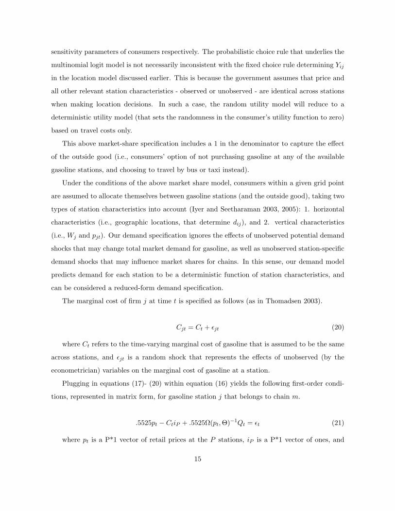
The marginal cost of firm j at time t is specified as follows (as in Thomadsen 2003).

Cjt = Ct + εjt (20)

where Ct refers to the time-varying marginal cost of gasoline that is assumed to be the same

across stations, and εjt is a random shock that represents the effects of unobserved (by the

econometrician) variables on the marginal cost of gasoline at a station.

Plugging in equations (17)- (20) within equation (16) yields the following first-order condi-

tions, represented in matrix form, for gasoline station j that belongs to chain m.

.5525pt − CtiP + .5525Ω(pt,Θ)−1Qt = εt (21)

where pt is a P*1 vector of retail prices at the P stations, iP is a P*1 vector of ones, and

15

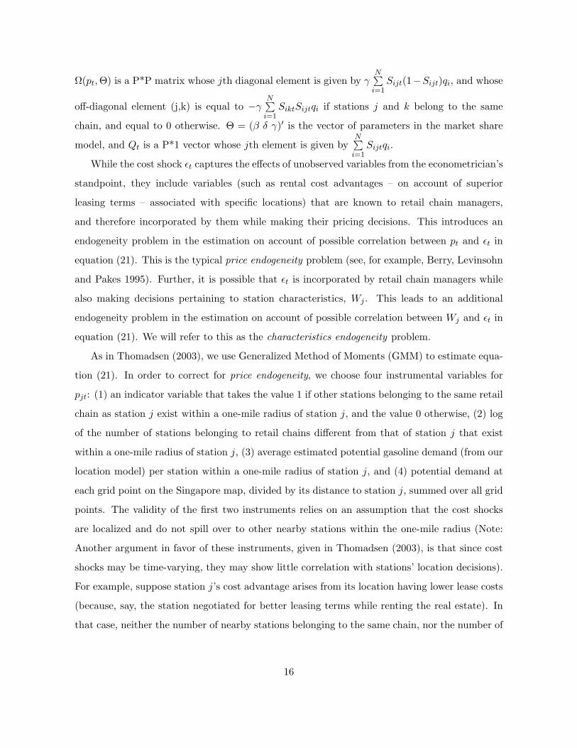
Ω(pt,Θ) is a P*P matrix whose jth diagonal element is given by γN∑

i=1Sijt(1−Sijt)qi, and whose

off-diagonal element (j,k) is equal to −γN∑

i=1SiktSijtqi if stations j and k belong to the same

chain, and equal to 0 otherwise. Θ = (β δ γ)′ is the vector of parameters in the market share

model, and Qt is a P*1 vector whose jth element is given byN∑

i=1Sijtqi.

While the cost shock εt captures the effects of unobserved variables from the econometrician’s

standpoint, they include variables (such as rental cost advantages – on account of superior

leasing terms – associated with specific locations) that are known to retail chain managers,

and therefore incorporated by them while making their pricing decisions. This introduces an

endogeneity problem in the estimation on account of possible correlation between pt and εt in

equation (21). This is the typical price endogeneity problem (see, for example, Berry, Levinsohn

and Pakes 1995). Further, it is possible that εt is incorporated by retail chain managers while

also making decisions pertaining to station characteristics, Wj . This leads to an additional

endogeneity problem in the estimation on account of possible correlation between Wj and εt in

equation (21). We will refer to this as the characteristics endogeneity problem.

As in Thomadsen (2003), we use Generalized Method of Moments (GMM) to estimate equa-

tion (21). In order to correct for price endogeneity, we choose four instrumental variables for

pjt: (1) an indicator variable that takes the value 1 if other stations belonging to the same retail

chain as station j exist within a one-mile radius of station j, and the value 0 otherwise, (2) log

of the number of stations belonging to retail chains different from that of station j that exist

within a one-mile radius of station j, (3) average estimated potential gasoline demand (from our

location model) per station within a one-mile radius of station j, and (4) potential demand at

each grid point on the Singapore map, divided by its distance to station j, summed over all grid

points. The validity of the first two instruments relies on an assumption that the cost shocks

are localized and do not spill over to other nearby stations within the one-mile radius (Note:

Another argument in favor of these instruments, given in Thomadsen (2003), is that since cost

shocks may be time-varying, they may show little correlation with stations’ location decisions).

For example, suppose station j’s cost advantage arises from its location having lower lease costs

(because, say, the station negotiated for better leasing terms while renting the real estate). In

that case, neither the number of nearby stations belonging to the same chain, nor the number of

16

nearby stations belonging to competing chains, is likely to be a function of such a cost advantage

of station j. In other words, instruments 1 and 2 will be uncorrelated with the cost shock. How-

ever, these instruments will be highly correlated with the price at station j to the extent that

station j will be less aggressive while setting price in the presence of other stations belonging

to the same chain (to avoid cannibalizing sales of the same chain’s stores), and more aggressive

while setting price in the presence of competitors. Our reduced-form price regressions (reported

in the appendix) show that instruments 1, 2 and 3 are indeed highly correlated with the observed

prices. Similarly, since the average estimated potential gasoline demand at nearby stations (i.e.,

instrument 3) depends only on observed demographic characteristics of the neighborhood (as

specified under the location model), instrument 3 will also be uncorrelated with the cost shock.

Finally, the rationale for the fourth instrumental variable is that it is a more global measure of

competitive effects compared to the first three instrumental variables that capture local effects

of competition. Further, it takes into account both how far away a competing station is as well

as the intensity of gasoline demand in that station’s neighborhood. Suppose Ut denotes a P*18

matrix, where each row represents a different station, and the 18 columns represent 1 intercept,

2 indicator variables for time t (representing 3 waves of data collection), 5 indicator variables

for chain (representing the 6 chains), 6 variables representing station characteristics (as will

be explained later), and 4 instrumental variables (as discussed above), the following moment

condition then underlies the GMM estimation (ignoring characteristics endogeneity).

E(εt|Ut) = 0 (22)

When the station characteristics correlate with the cost shocks, the moment condition in

equation (22) is invalid. We are unable to find appropriate additional instruments in order to

correct for characteristics endogeneity. Therefore, we re-estimate our proposed model by exclud-

ing the station characteristics as explanatory variables within Wj , and as instruments within

Ut, thereby precluding concerns about possible endogeneity of such variables in the estimation.

We compare the estimates of the travel cost (δ) and price sensitivity (γ) parameters obtained

using this modified specification to those obtained using our original specification. This allows

us to understand the robustness of these two parameter estimates, i.e., their sensitivity (or lack

thereof) to the inclusion of possibly endogenous station characteristics in the estimation.

17

Under this specification of the pricing model, observed price variations in the data arise on

account of differences in demand characteristics across stations, time-varying cost changes (that

are equal across stations), as well as cost shocks at the station-level. Last, but not the least,

potential gasoline demand at a grid point, i.e., qi, is not observed in the data. We use the

estimated potential gasoline demand in grid point i, obtained using the estimates of the location

model, as a proxy for qi. This allows the potential gasoline demand to be not only simultaneously

determined by local population, median income, number of cars owned, presence of highway and

downtown, but also lets the weights associated with these factors be endogenously estimated

from the observed distribution of gasoline stations. This also relieves us from the burden of

having to estimate potential gasoline demand (in addition to the parameters of the pricing

model) from the price data.

Identification Issues and Caveats

It is useful to discuss some identification issues. We identify marginal costs from the average

price across all stations, and the changes in this average price across time periods (i.e., waves).

Although station-level demand is not observed in the data, we are able to identify the same

by invoking the equilibrium conditions of demand and supply. What identifies the demand

function is sufficient systematic variation in prices in the data across stations that reside in

neighborhoods with different levels of local potential gasoline demand and different levels of

local competitive intensity. Proof of sufficient variation in prices is easily observed in the results

of our reduced-form pricing regressions (reported in the appendix), where we find the effects

of all the competitive environment factors to be significant. For example, suppose a station

that faces little local competition (i.e., few nearby stations) prices higher than another station

that faces higher local competition (i.e., many nearby stations), for the same level of local

potential gasoline demand, this would serve as the source of identification for the travel cost

and price sensitivity parameters in the demand function. Suppose two stations belonging to

different chains price differently within the same local market, this would serve as the source of

identification of the brand intercepts in the demand function.

Three caveats are in order. First, since we rely on price data to infer both cost-side as well

as demand-side parameters, our estimates of demand are likely to be less efficient compared to

18

estimates obtained using demand data. Second, since we rely on specific assumptions such as

Bertrand price competition between retail chains, and Multinomial Logit demand for gasoline

stations, in order to achieve this identification, it is possible that our estimates are subject to

mis-specification bias. Third, although we allow for unobserved demand shocks in potential

gasoline demand, qit, we ignore such unobserved demand shocks in the market share function,

Sijt. In this regard, we reiterate that these assumptions are dictated by the fact that we do not

have access to demand data in the product category.

Description of Data

Our data pertains to the gasoline market in Singapore. This market is a good geography

for examining firm conduct for a variety of institutional considerations. First, it is a self-

contained market of substantial size. For instance, 2002 gasoline sales alone were in excess

of a billion liters and, more infamously, Singapore ranks second (next to the U.S.) in global

carbon dioxide emission per unit of GDP (Economist, May 9, 2003). Second, all the demand is

supplied by local refiners and there is no possibility of supply-side leakage. Motorists crossing

the borders into Malaysia (the only possible road transit) are required by law to have their

gas-tanks filled to at least three-quarters prior to crossing the border. Hence, supply-demand

leakages due to the price differences between the two markets do not hold.4 Third, the market is

increasingly viewed as being a mature and competitive market. Gasoline demand is stable and

expected to grow slowly due to the controlled increase in automobile ownership. Traditionally,

retail competition was conducted through non-price instruments (sweepstakes, freebies, loyalty

programs). Price promotions are a recent addition (past three to five years) to this mix and are

becoming increasingly common and distributed across the entire island. Currently, upwards of

25% of gasoline stations are running promotions ranging in depth from 5% to 15% on petrol

and/or diesel. Fourth, the oil majors control all elements of their channel from production to

distribution to retailing. However, the location decisions for retail outlets are decided by the

URA (Singapore’s Urban Redevelopment Authority).

We employ survey data, representing a cross-section of 226 gasoline stations in Singapore4The price differential between the two countries is substantial. The price of a liter of 98-octane petrol in

May 2002 was 1.244 S$ in Singapore and .630 S$ in Malaysia (prices are in Singaporean dollars). The substantialgasoline tax revenues was suggested to the authors as one of reasons for the Singaporean ordinance.

19

during late 2001 and early 2002. We include all gasoline stations in mainland Singapore in our

empirical analyses, ignoring gasoline stations that are located in islands off the Singapore coast.

There are a total of 229 gasoline stations in mainland Singapore. We had to exclude three

stations - two belonging to Mobil and one to BP - whose geographic locations were missing

in the survey data. Among the 226 stations in mainland Singapore, 75 stations are owned

by Shell, 43 by Mobil, 39 by Esso, 32 by Caltex, 29 by BP, and 8 by SPC. The survey data

include, for each gasoline station, the prices of four grades - Premium, 98UL, 95UL and 92UL

- of petrol, the price of diesel, as well as a large number of station-specific characteristics,

e.g. number of pumping bays, presence of convenience store, pay-at-pump facility, car wash,

service station, ATM, store hours, prices of goods at convenience store etc. Our dataset also

contains demographic information - population, home ownership, age, employment status, mode

of transportation, income etc. - pertaining to each gasoline station’s market. Three waves of

data collection - all of which used the same survey instrument - were undertaken at the same

set of 226 gasoline stations during the months of November 2001, December 2001 and January

2002. This yielded some time-series variation in gasoline prices. Since 98UL is the most popular

grade of gasoline in Singapore, we report the estimation results for our pricing model based on

this grade of gasoline. Estimation results for the other grades are consistent with those obtained

for the 98UL grade, and are available from the authors.

For the location model, we divide mainland Singapore into a rectangular grid of 1550 grid

points that are equally spaced both in the horizontal and vertical dimensions. Picking 1550

as opposed to a smaller number of grid points ensures that each grid point has no more than

one gasoline station, which is required to be consistent with our location model (see equations

1-6). Estimating the location model enables us to endogenously characterize potential gasoline

demand at each grid point in Singapore. We allow the following demographic characteristics

to influence local potential gasoline demand at each grid point (i.e., qi). (1) POPi, the local

population represented within grid point i, computed as the total population of the census tract

to which the grid point belongs divided by the total number of grid points within that census

tract; (2) INCi, the median income of the census tract to which grid point i belongs; (3) CARi,

the total number of cars represented within grid point i, computed as the total number of cars

within the census tract to which the grid point belongs divided by the total number of grid

20

points within that census tract; (4) AIRi, an indicator variable that takes the value 1 if grid

point i is located adjacent to the airport, and 0 otherwise; (5) DTi, an indicator variable that

takes the value 1 if grid point i is located within the downtown area, and 0 otherwise; (6) HWYi,

an indicator variable that takes the value 1 if grid point i is located adjacent to a major highway,

and 0 otherwise.

For the pricing model, we use the same set of 1550 grid points as in the location model in

order to compute aggregate demand for each gasoline station (see equation 17). We also plug the

estimated values of qi from the location model directly into equation (18) while estimating the

pricing model. We allow the following station characteristics (Wj) to influence market shares for

gasoline stations (i.e., Sij) in equation 19: (1) CHAINj , a five-dimensional vector of indicator

variables representing which of six different retail chains station j belongs to; (2) PUMPSj , the

total number of gasoline pumping bays available in station j; (3) PAYj , an indicator variable

that takes the value 1 if STATION j has pay-at-pump facility, and 0 otherwise; (4) HOURSj ,

an indicator variable that takes the value 1 if station j is open 24 hours a day, and 0 otherwise;

(5) WASHj , an indicator variable that takes the value 1 if station j has a car wash facility, and

0 otherwise; (6) SERVj , an indicator variable that takes the value 1 if station j has a service

station, and 0 otherwise; (7) DELIj , an indicator variable that takes the value 1 if station j has

a specialty deli, and 0 otherwise.

The variable PUMPSj is observed to vary from 4 to 20 across stations in our dataset. The

remaining indicator variables - PAYj , HOURSj , WASHj , SERVj and DELIj - are observed

to take the value 1 for 69, 88, 50, 52 and 22 percent of the stations in our dataset respectively.

In addition to the above station characteristics, the market share model also includes the price

of gasoline at station j, PRICEj , as well as travel distance, dij , as explanatory variables (see

equation 19).

Given in Table 1 are the means and standard deviations of prices of 98UL gasoline, the

most popular grade of gasoline in Singapore, at various retail chains in Singapore. The average

price of 98UL gasoline is about 5 cents lower at SPC compared to the other retail chains. The

standard deviation of price of gasoline is about .03 cents (for most grades and retain chains),

which is much smaller than the standard deviation of price observed in US markets (see, for

example, Shepard 1991, Iyer and Seetharaman 2003 etc.). This price variation includes variation

21

across stations within a chain, as well as across time.

Empirical Results

We report the estimates of our proposed location model (called PROPOS) in column 2 of Table

2. The standard errors associated with these estimates are reported in columns 3 and 4, and are

obtained, using a bootstrapping procedure, as follows: Based on the estimate α, we generate

the empirical distribution of ej , using equation (9), as the difference between the observed and

predicted locations. Using this empirical distribution of errors, as well as the estimate α, we

simulate locations for the gasoline stations. Taking these simulated locations as actual locations,

we re-estimate the proposed location model. We then cycle through the same procedure again.

We do this until we have 50 sets of α, based on which we compute the standard deviation.

The results show that, as expected, potential gasoline demand at a grid point is a positive

function of the population, median income and number of cars owned in the local neighborhood.

This validates our earlier contention that population is only one among several demographic

variables that influence local demand for gasoline. We also find, as expected, that proximity to

the airport, downtown and highways increase local potential gasoline demand, with proximity to

highways accounting for the largest increase. All of these results are intuitively sensible and give

excellent face validity to our proposed location model. We also estimate a benchmark model

(called BENCH) that restricts potential gasoline demand to be equal to the local population (as

in, say, Seim 2002). In order to understand how well we are able to predict observed gasoline

station locations using our chosen set of six demographic variables, we compare the predictive

ability of PROPOS to that of BENCH. The quasi mean-squared error based on PROPOS is

7210, while that based on BENCH is 15199, thus indicating more than 50% predictive gains

from using demographic variables to predict local potential gasoline demand as in our proposed

location model.

Figure 1 visually represents the estimated local potential gasoline demand across grid points

on the Singapore map. Overlaying the distribution of estimated potential gasoline demand

across grid points on top of the observed distribution of gasoline stations across the same set

of grid points enables us to visually convey the government’s basis for placing large number

of gasoline station locations at some geographic neighborhoods and not at others. In order to

22

facilitate interpretation, we code Figure 1 into four (equal-sized) regions of varying shades (from

light to dark) – low demand (lightest shade), middle demand I (lighter shade), middle demand

II (light shade), high demand (dark shade) – using the quartiles of the estimated distribution

of potential gasoline demand. The dense cluster of observed gasoline stations in the north-east

portion of Figure 1, along with the estimated high degree of potential gasoline demand in this

part of the map, is a consequence of three effects: the presence of downtown in the horizontal line

spanning (380,380) to (620,380), the presence of the airport close to (700,350), and the presence

of a major highway spanning the region (700,420) to (800,400). Overall there appears to be a

good degree of agreement between the estimated locations and the actual locations of the 226

stations. For example, our estimated locations are also highly concentrated in the north-east

portion of Figure 1.

In Table 3 we present the results of the pricing model for 98UL gasoline. In this table, the

second column excludes station characteristics as explanatory variables within Wj (in order to

address the issue of characteristics endogeneity, as discussed earlier), while the third column

includes such variables. Understandably, the minimized criterion function value is lower under

column 3 (since it includes additional explanatory variables) than under column 2, but the

estimates of common parameters are similar to each other. The estimated price-cost margins

from columns 2 and 3 are 21.3% and 21.2% respectively. These are higher than estimated

margins in the North American gasoline market. For example, Manuszak (1999) estimates retail

price-cost margins in Hawaiian gasoline stations to be about 10%.. This perhaps reflects lower

intensity of price competition in the Singapore market. In fact, price promotions were long absent

in the Singapore market, and became a prevalent retail activity only recently, as discussed in

the Euromonitor report for 2004. In terms of intrinsic brand preferences of consumers (reflected

in the estimated brand intercepts in the demand model), we allow these preferences to have two

components: (1) one component that is common across all brands (called CONSTANT in Table

3), representing consumers’ baseline preferences for gasoline brands relative to the outside good,

and (2) another component (reported separately under each brand name in Table 3) representing

consumers’ additional preference for each brand relative to SPC (for identification purposes).

The component that is shared by all brands (CONSTANT) – and must be interpreted as the

baseline preference for each brand relative to the outside good – is found to be insignificantly

23

different from zero. BP appears to be the strongest brand in the market place (since it has the

highest estimated intercept). The coefficients associated with both price and travel distance are

negative and significant (-2.845 and -.103 under column 2, -2.808 and -.106 under column 3).

This implies that both price and travel distance are important considerations for consumers when

they choose between gasoline stations, which is intuitively pleasing since this underscores the

importance of locations in firms’ pricing decisions. The price sensitivity and travel cost estimates

translate into the following substantive interpretation (under both pricing models): Consumers

will be willing to travel an extra mile to save about 3 cents per liter of gasoline. Assuming

an average purchase of gasoline in Singapore to involve 40 liters of gasoline, this implies that

consumers would save about $1.3 by traveling that extra mile. Under the same assumption, the

highest estimated brand intercept for BP translates to the following substantive interpretation:

Compared to SPC, BP would be able to command a price premium of 4 cents per liter while

still keeping the consumer indifferent between the two brands. We find that including station

characteristics, as in column 3, does not substantively change any of the estimates reported

in column 2. However, on account of our inability to explicitly address potential endogeneity

issues pertaining to station characteristics in the pricing model (as discussed earlier), we do not

attempt to directly interpret the estimated parameters associated with such characteristics.

Policy Implications

Estimated Market Shares and Profits

Based on the estimated parameters, we compute the weekly market shares, and therefore profits

(computed at observed prices), of the six retail chains in our dataset. For the market share

computation, we use the price data collected from the first wave. For the profit computation,

we assume the total weekly demand for petrol to be 18 million liters. This is arrived at as

follows: The reported annual retail sales of petrol in Singapore for 2001 was S$1.149 bil., which

is equivalent to S$22 mil. a week. Assuming an average retail price of S$1.234 per liter, this

translates to 18 mil. liters. The results are reported in Table 4. The estimated market shares

agree remarkably well with corresponding reported market shares of 33.0% (Shell), 14.2% (Cal-

tex), 35.2% (Exxon-Mobil), 13.7% (BP) and 3.9% (SPC) for 2002. This lends excellent face

validity to our parameter estimates. Among the six retail chains, the most profitable chain is

24

estimated to be Shell with an estimated profit of $7.13 mil. per week, while the least profitable

is SPC with an estimated profit of $.85 mil.

In Figure 1, we also identify the most and least profitable stations in Singapore (based on

the estimated parameters). The most profitable station is run by Shell (with estimated weekly

profits of S$30,000) and is located in the densest neighborhood in Singapore in terms of potential

gasoline demand, which suggests that competitive pressures do not dissipate the profitability of

“prime real estate ”. This lends further evidence to the popular emphasis in retailing of “location,

location, location! ”The least profitable station is run by SPC (with estimated weekly profits

of S$23,000) and is located in a remote neighborhood in Singapore that is estimated to have

low potential gasoline demand. The estimated weekly sales for the most and least profitable

stations are S$138,000 and S$92,000 respectively. These numbers are very much in the vicinity

of publicly available weekly average sales figures (reported by Euromonitor) of S$114,000 and

S$85,500 for large and small petrol stations in Singapore. According to the Euromonitor report,

average weekly retail sales of large and small stations for 2002 were S$140,000 and S$105,000

respectively, with gasoline accounting for 81.5% of retail sales. This yields weekly average petrol

sales of S$114,000 and S$85,500 respectively. One reason for why our estimated numbers are

higher than the reported numbers may be that we have used a premium (i.e., higher priced)

grade of gasoline (98UL) in our computations.

Merger Simulation

In July 2004, SPC announced that it would acquire all petrol stations from BP, after the latter

had decided to exit from the petrol retail market in Singapore. In September 2004, SPC an-

nounced that the acquisition was complete. SPC also announced that it will continue to retain

the BP brand name for the BP stations, gradually changing the names of these stations to SPC

in a phased manner over time. We consider the effects of this merger scenario by running an ap-

propriate simulation using our estimated parameters. Specifically, we simulate the equilibrium

market shares, and therefore, equilibrium prices, of the 226 stations after assuming that the 8

stations owned by SPC merge with the 29 stations owned by BP, thus belonging to a single chain

that maximizes the sum of profits across 37 stations. Since our estimation results show that BP

is the most preferred brand, while SPC is one of the least preferred brands, in the Singapore

25

petrol market (as evidenced by the estimated brand intercepts in Table 4), and to be consistent

with the “post-merger”scenario described above, we make two alternative assumptions: 1. Each

station retains its previously held brand name (i.e., SPC or BP), or 2. All BP stations are

renamed with the SPC brand name. We will refer to these two assumptions as SCENARIO 1

and SCENARIO 2 respectively.

We face a technical issue in conducting this policy experiment. We have to calculate equi-

librium prices of 226 firms following the merger. This involves a “fixed point ”computation that

is based on the following equilibrium condition.

.55pt − CtiP + .55Ω(pt, Θ)−1Qt = 0 (23)

The dimensionality of the fixed points is too large to be computed using conventional “hill-

climbing”derivative methods or the simplex method. To solve the problem, we employ the

following contraction mapping algorithm.

ˆpn+1 = pn + ∆[.55pn − CtiP + .55Ω(pn, Θ)−1

Qt] (24)

where n = 0, 1, ... is the iteration number, ∆ ∈ [0, 1] is a contraction factor. The iterative

algorithm converges when dn < ε, where dn = Max|pn+1 − pn|, and ε is a pre-determined

tolerance level. The algorithm converges very quickly to within the tolerance level, as long as

∆ < 1. We experimented with several values of ∆ in the [0,1] range, and initial values p0, in

order to ensure that the computed fixed points were unique and insensitive to our choice of ∆

and initial values. The algorithm always converged to a unique fixed point as long as ∆ < 1.

Table 5 presents the equilibrium prices, market shares and profits under the pre-merger

scenario, as well as under the two post-merger scenarios (i.e., SCENARIO 1 and SCENARIO

2). Average prices at all chains are found to increase from 2 to 7 cents under the merger (under

both post-merger scenarios), which suggests that the merger will reduce the intensity of price

competition in the Singapore market. The price increase under both post-merger scenarios are

roughly the same for all chains except for BP, for which the price increase under SCENARIO 2 is

much smaller (i.e., 1 cent, or .6%) compared to that under SCENARIO 1 (i.e., 6 cents, or 4.7%).

The reason for this is that since the estimated brand preference for BP is higher than that of

SPC, BP stations stand to lose some pricing power by forfeiting the stronger brand name after

26

the merger and adopting the weaker name instead. In fact, this also leads to decreased profits

for BP under SCENARIO 2. Since BP stations price lower under SCENARIO 2 than under

SCENARIO 1, the other chains also price somewhat less than they would under SCENARIO

1, on account of competitive pressures. Specifically, the increase in equilibrium prices for Shell,

Caltex, Esso and Mobil are 3.7%, 2.2%, 4.8% and 3.0% respectively under SCENARIO 1, and

4.1%, 2.6%, 5.2% and 3.4% respectively under SCENARIO 2. Profits are found to increase for

all chains under SCENARIO 1, while they increase for all chains except BP under SCENARIO

2. Market shares for BP and SPC are found to decrease after the merger. However, the increase

in their prices more than offsets this effect from a profit standpoint. The profit decrease for BP

under SCENARIO 2 is on account of BP stations disadopting their (strong) brand name and

adopting the relatively weak brand name of SPC instead. In fact, this decrease profit is strong

enough to decrease the combined profit of SPC and BP compared to its pre-merger counterpart.

Overall, these results suggest that the merger will lead to increased profits, and decreased price

competition among all the firms in the petrol industry. Given our findings under SCENARIO

2 about profits decreasing for BP stations, it is indeed wise that SPC is not changing the name

of existing BP stations to SPC immediately after the merger. Our policy experiment assumes

the cost structure of the industry, as well as consumers’ brand preferences, to remain unchanged

after the merger. It is quite possible that these parameters may change in the long run after the

merger. For example, consumers’ preference for the SPC brand name may strengthen gradually

as it gains a larger presence in the Singapore gasoline market. At this point, a caveat is in

order. Our demand model does not allow for the possibility that SPC buyers may be more price

sensitive than buyers of other brands of gasoline. If that is indeed the case, it is possible that

the post-merger prices of SPC may be lower than what is predicted in our policy simulations.

Investigating this issue, however, is beyond the scope of our paper since we have access to

neither consumer demand data nor long time series data (with significant temporal variations)

on gasoline prices.

Conclusions

In this paper, we propose and estimate a econometric model of location and pricing decisions

of gasoline stations in the Singapore market. Our location model, the first of its kind and the

27

first to be estimated for gasoline markets, is built on the premise that the Singapore government

determines optimal retail locations for gasoline stations on the basis of maximizing social welfare

of Singapore residents by minimizing their travel costs. This is an important methodological

contribution of our work. Our conditional pricing model is built on the premise of Bertrand

competition between gasoline retail chains.

By estimating our proposed location model using empirical data on actual geographic lo-

cations of gasoline stations, we are able to quantify the explicit dependence of local potential

gasoline demand on the following local demographic characteristics of the neighborhood: pop-

ulation, median income, number of cars, proximity to airport, downtown and highways. Using

the estimated category-level demand at each local neighborhood in Singapore as an input, we

then estimate our proposed pricing model using empirical data on actual prices of gasoline at

various stations. We find retail margins for gasoline to be about 21%, and that market share for

a gasoline station is negatively influenced by the price of gasoline as well as travel cost. We find

that consumers are willing to travel up to a mile for a price saving of 3 cents per liter (which

translates to a saving of about $1.3 on a 40-liter tank of gasoline).

We use our estimates to calculate the relative profitability of various retail chains, identify the

most and least profitable gasoline stations in Singapore, as well as perform a policy experiment

relating to the merger of SPC and BP during the latter part of 2004. We find that prices and

profits of all firms in the Singapore petrol industry will increase in response to this merger.

We believe that our effort at estimating cost and demand parameters from price data, using

an econometric model of pricing, is valuable from the standpoint of obtaining a preliminary

understanding of the Singapore gasoline market. Taken together with our location model, our

estimation methodology and results can be used to answer policy questions of interest to both

firms and policy-makers. For example, our results highlight the importance of factors such as

proximity to highway, airport and downtown in terms of influencing potential gasoline demand.

Furthermore, our methodology can be used to throw light on how gasoline prices at various

stations would change in response to mergers and acquisitions. We hope that our work spurs

future research on gasoline markets.

At this point, some caveats are in order. First, we use the current census data, and the

demographic information therein, to understand the demographic drivers of the Singapore gov-

28

ernment’s decisions pertaining to gasoline stations’ locations that were made over a long period of

time. Locating and employing the census data from several periods would be useful to check the

robustness of our estimation results. Second, our location model is built on the assumption that

the Singapore government decides the locations and assumes prices to be equal across gasoline

stations. While this does seem reasonable in our case (based on our conversations with public

policy planners with Singapore), it would be of research interest to investigate the consequences

of relaxing these assumptions. For example, in some cases (such as supermarket retailing in the

US), retail chains may choose locations for their stores with the objective of maximizing total

profits across all their stores. This may involve the consideration of the strategic impact of the

firm’s location decisions on competing chains’ location decisions. Handling such an extension

of our model, while it poses a computationally non-trivial challenge, is an important avenue

for future research since it would usefully apply to many business problems. Third, our pric-

ing model assumes immediate adjustment of retail prices to cost changes, although empirical

findings suggest that gasoline prices respond slowly to cost changes (Borenstein, Cameron and

Gilbert 1997, Borenstein and Shepard 2002). We are unable to address this issue because of the

limited time series (i.e., three waves) of prices that is represented in our dataset. It is difficult

to accommodate the lagged effects of cost changes using just three temporal observations at the

station-level. Fourth, our pricing model ignores the effects of firm-specific unobserved demand

shocks in the market share function. Given that we have access to pricing data only, and do

not have demand data, relaxing this assumption is difficult. The GMM methodology will be

difficult to apply since the demand shocks will enter the pricing equation non-linearly.

29

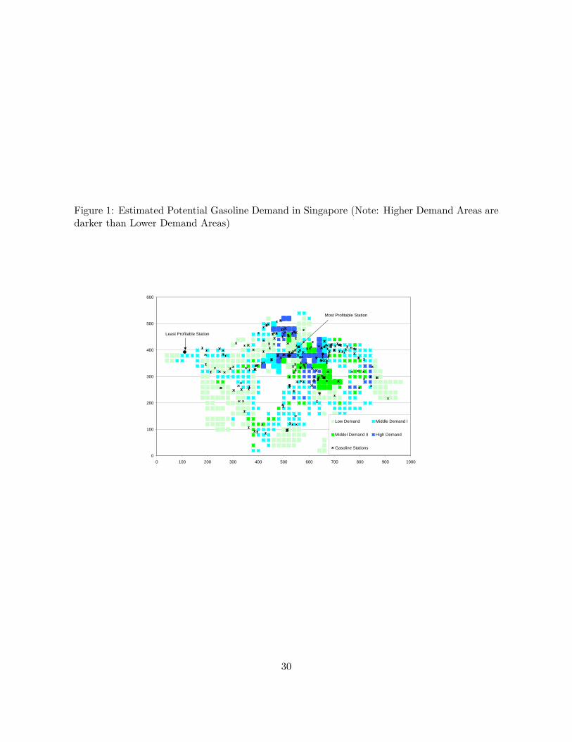
Figure 1: Estimated Potential Gasoline Demand in Singapore (Note: Higher Demand Areas aredarker than Lower Demand Areas)

0

100

200

300

400

500

600

0 100 200 300 400 500 600 700 800 900 1000

Low Demand Middle Demand I

Middel Demand II High Demand

Gasoline Stations

Most Profitable Station

Least Profitable Station

30

Table 1: Means and Standard Deviations of 98UL Gasoline Prices at Various Retail Chains.

Chain Mean Price Std. Dev. of Price

Shell 1.19 .03Caltex 1.18 .04

Esso 1.19 .03Exxon − Mobil 1.19 .03

BP 1.19 .03SPC 1.14 .03

Table 2: Estimated Parameters of the Location Model (Capturing the Effects of Local MarketCharacteristics on Potential Demand for Gasoline).

Parameter Estimate Std. Error

POPi 2.3425 .2042INCi 2.5327 .0995CARi .9462 .0975AIRi 1.8075 .0900DTi 1.8394 .1063

HWYi 2.9434 .0332

31

Table 3: Estimated Parameters of the Pricing Model (standard errors within parentheses) (Cap-turing the Effects of Station Characteristics on Station-Level Demand for Gasoline).

Parameter Model 1 Model 2COST

Constant .415 (.009) .417 (.027)Wave2 -.019 (.001) -.020 (.000)Wave3 .000 (.002) -.001 (.001)

DEMANDConstant .115 (22.402) .049 (9693.489)

Shell -.062 (.038) -.058 (.023)Caltex .052 (.022) .057 (.020)

Esso .063 (.027) .069 (.025)Mobil .039 (.028) .049 (.024)

BP .116 (.023) .127 (.028)PUMPSj na .002 (.000)

PAYj na .002 (.001)HOURSj na -.032 (.004)WASHj na .005 (.001)SERVj na -.009 (.001)DELIj na -.012 (.002)

PRICEj -2.845 (.086) -2.808 (.381)DISTij -.103 (.003) -.106 (.014)

CriterionFn.V alue .0028 .0021

Table 4: Estimated Market Shares, Actual 2002 Market Shares, and Estimated Profits of FiveRetail Chains in Singapore.

Chain Estimated Share Actual Share Estimated Profit

Shell 32.9% 33.0% $7.13 mil.Caltex 14.5% 14.2% $3.13 mil.

Exxon-Mobil 36.1% 35.2% $7.83 mil.BP 12.6% 13.7% $2.73 mil.

SPC 3.9% 3.9% $.85 mil.

32

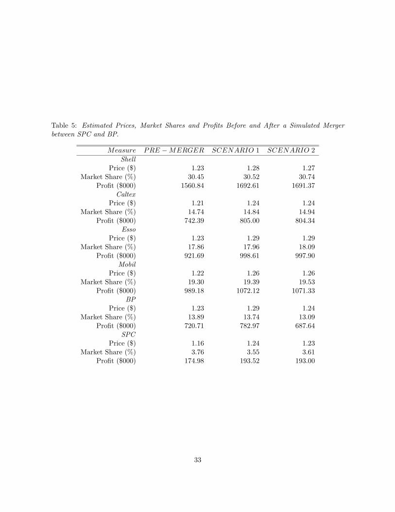
Table 5: Estimated Prices, Market Shares and Profits Before and After a Simulated Mergerbetween SPC and BP.

Measure PRE − MERGER SCENARIO 1 SCENARIO 2Shell

Price ($) 1.23 1.28 1.27Market Share (%) 30.45 30.52 30.74

Profit ($000) 1560.84 1692.61 1691.37Caltex

Price ($) 1.21 1.24 1.24Market Share (%) 14.74 14.84 14.94

Profit ($000) 742.39 805.00 804.34Esso

Price ($) 1.23 1.29 1.29Market Share (%) 17.86 17.96 18.09

Profit ($000) 921.69 998.61 997.90Mobil

Price ($) 1.22 1.26 1.26Market Share (%) 19.30 19.39 19.53

Profit ($000) 989.18 1072.12 1071.33BP

Price ($) 1.23 1.29 1.24Market Share (%) 13.89 13.74 13.09

Profit ($000) 720.71 782.97 687.64SPC

Price ($) 1.16 1.24 1.23Market Share (%) 3.76 3.55 3.61

Profit ($000) 174.98 193.52 193.00

33

References

Berry, S., Levinsohn, J., Pakes, A. (1995). Automobile Prices in Market Equilibrium, Econo-metrica, 63, 4, 841-890.

Borenstein, S., Cameron, A.C., Gilbert, R. (1997). Do Gasoline Prices Respond Asymmetri-cally to Crude Oil Price Changes?, The Quarterly Journal of Economics, 112, 1, 305-339.

Borenstein, S., Shepard, A. (2002). Sticky Prices, Inventories and Market Power in WholesaleGasoline Markets, RAND Journal of Economics, 33, 1, 116-139.

Daskin, M.S. (1995). Network and Discrete Location, John Wiley and Sons: New York.

Davis, P. (2001). Spatial Competition in Retail Markets: Movie Theaters, Working paper,MIT Sloan School of Management.

Choi, S.C., Desarbo, W.S., Harker, P.T. (1990). Product Positioning under Price Competition,Management Science, 36, 2, 175-199.

D’Aspremont, C., Gabszewics, J., Thisse, J.F. (1979). On Hotelling’s Stability in Competition,Econometrica, 17, 1145-1151.

Dube, J.P., Sudhir, K., Ching, A., Crawford, G.S., Draganska, M., Fox, J.T., Hartmann, W.,Hitsch, G.J., Viard, V.B., Villas-Boas, M., Vilcassim, N.J. (2005). Recent Advances inStructural Econometric Modeling: Dynamics, Product Positioning and Entry, MarketingLetters, forthcoming.

Goolsbee, A., Petrin, A. (2004). The Consumer Gains from Direct Broadcast Satellites andthe Competition with Cable TV, Econometrica, 72, 2, 351-381.

Hauser, J.R. (1988). Competitive Price and Positioning Strategies, Marketing Science, 7, 1,76-91.

Hauser, J.R., Shugan, S.M. (1983). Defensive Marketing Strategies, Marketing Science, 2, 4,319-360.

Hotelling, H. (1929). Stability in Competition, Economic Journal, 39, 153, 41-57.

Iyer, G.K., Seetharaman, P.B. (2003). To Price Discriminate or Not: Product Choice and theSelection Bias Problem, Quantitative Marketing and Economics, 1, 2, 155-178.

Iyer, G.K., Seetharaman, P.B. (2005). Quality and Location in Retail Gasoline Markets, Work-ing paper, Walter A. Haas School of Business, University of California at Berkeley.

Manuszak, M.D. (1999). Firm Conduct in the Hawaiian Petroleum Industry, Working paper,Graduate School of Industrial Organization, Carnegie Mellon University, Pittsburgh.

Mazzeo, M. (2002). Product Choice and Oligopoly Market Structure, RAND Journal of Eco-nomics, 33, 2, 1-22.

34

McManus, B. (2003). Nonlinear Pricing in an Oligopoly Market: The Case of Specialty Coffee,Working paper, John M. Olin School of Business, Washington University, St. Louis.

McFadden, D.L. (1974). The Measurement of Urban Travel Demand, Journal of Public Eco-nomics, 3, 4, 303-328.

Moorthy, K.S. (1988). Product and Price Competition under Duopoly, Marketing Science, 7,2, 141-168.

Nelder, J.A., Mead, R. (1965). A Simplex Method for Function Minimization, ComputationalJournal, 7, 308-313.

Pakes, A., Pollard, D. (1989). Simulation and the Asymptotics of Optimization Estimators,Econometrica, 57, 5, 1027-1057.

Phibbs, C.S., Luft, H.S. (1995). Correlation of Travel Time on Roads Versus Straight LineDistance, Medical Care Research and Review, 52, 4, 532-542.

Pinkse, J., Slade, M.E., Brett, C. (2002). Spatial Price Competition: A Semiparametric Ap-proach, Econometrica, 70, 3, 1111-1153.

Png, I., Reitman, D. (1994). Service Time Competition, RAND Journal of Economics, 25, 4,619-634.

Seim, K. (2004). An Empirical Model of Firm Entry with Endogenous Product-Type Choices,Working paper, Graduate School of Business, Stanford University.

Shepard, A. (1991). Price Discrimination and Retail Configuration, Journal of Political Econ-omy, 99, 1, 30-53.

Slade, M.E. (1992). Vancouver’s Gasoline-Price Wars: An Empirical Exercise in UncoveringSupergame Strategies, The Review of Economic Studies, 59, 2, 257-276.

Syverson, C. (2004). Market Structure and Productivity, Journal of Political Economy, 112, 6,1181-1222.

Thomadsen, R. (2003). The Effects of Ownership Structure on Prices in Geographically Dif-ferentiated Industries, Working paper, Graduate School of Business, Columbia University.

Van Heerde, H.J., Leeflang, P.S.H., Wittink, D.R. (2000). The Estimation of Pre- and Post-Promotion Dips with Store-Level Scanner Data, Journal of Marketing Research, 37, 3,383-395.

35

Appendix

In order to get a qualitative understanding of market structure in the Singapore gasoline market,based on which we can make appropriate assumptions while specifying our structural pricingmodel, we ran the following linear regression model (which is the spirit of Goolsbee and Petrin2004) that uses the observed prices from the 226 gasoline stations, across 3 waves of datacollection, as 678 independent realizations of the dependent variable (conditional on differentsets of covariates).

pjt = Wjtβ + εjt (25)

where Wjt includes the following key covariates: (1) an indicator variable that takes thevalue 1 if other stations belonging to the same retail chain as station j exist within a one-mileradius of station j, and the value 0 otherwise (called SAME henceforth), (2) log of the numberof stations belonging to retail chains different from that of station j that exist within a one-mileradius of station j (called OTHER henceforth), and (3) average potential gasoline demand perstation within a one-mile radius of station j (called DEMAND henceforth),5. We also includeappropriate controls in the linear regression, i.e., time-specific and brand-specific fixed effects,as well as the effects of station characteristics. The results of this pricing regression are reportedin Table 6. While the second column of the table excludes station characteristics as controls inthe regression, the third column does not.

Substantive results are strikingly similar between the second and third columns of Table 6.We find that SAME has a positive effect on prices. This implies that prices at stations are higherif other stations belonging to the same retail chain are nearby, which suggests that retail chainsmay be engaged in maximizing the profits of the chain as a whole (as opposed to competingamong themselves in maximizing individual station profits). We find that OTHER has a negativeeffect on prices. This implies that as the number of stations belonging to competing chainsincreases in the vicinity, prices at the station are lowered. This suggests that chains may beengaged in price competition with each other, although stations within a chain accommodateeach other. We find that DEMAND has a negative effect on prices. This suggests that stations indenser neighborhoods try to lure more consumers to their stations by lowering their prices (withthe resultant impact on margins not being too much), while stations in sparser neighborhoodsmake profits off their margins. Alternatively, it is possible that low-cost stations self-select intodenser neighborhoods by bidding higher for those locations, which is responsible for the lowerprices observed in such neighborhoods (Syverson 2004).

The above estimation results suggest that (1) there exists price competition between retailchains in the Singapore gasoline market, and (2) gasoline stations try to avoid cannibalizingsales at nearby stations belonging to the same retail chain by not lowering prices too much.On the basis of these results, we assume in our structural pricing model that retail chains areengaged in Bertrand competition with each other, where each chain maximizes the combinedprofits from all its stations in Singapore.6 This is a standard assumption widely used in theempirical IO literature.

5This is based on the estimates of potential gasoline demand from the location model.6In fact, our estimating an alternative model of station-level Bertrand price competition explicitly shows that

it does not explain the observed prices as well as the chain-level model. These results are available from theauthors.

36

Parameter PricingModel1 PricingModel2Wave2 -.0500 (.0018) -.0500 (.0018)Wave3 -.0502 (.0018) -.0502 (.0018)

Shell 1.2280 (.0024) 1.2290 (.0043)Caltex 1.2201 (.0029) 1.2211 (.0043)

Esso 1.2294 (.0028) 1.2311 (.0047)Mobil 1.2279 (.0028) 1.2304 (.0048)

BP 1.2327 (.0032) 1.2348 (.0045)SPC 1.1832 (.0043) 1.1839 (.0053)

PUMPSj na .0004 (.0003)PAYj na -.0003 (.0020)

HOURSj na -.0058 (.0024)WASHj na .0013 (.0016)SERVj na -.0016 (.0017)DELIj na -.0026 (.0023)SAME .0037 (.0020) .0039 (.0019)

OTHER -.0029 (.0013) -.0026 (.0013)DEMAND -5.4E-6 (2.4E-6 -4.6E-6 (2.4E-6)

Table 6: Estimated Parameters of Reduced-Form Pricing Models (standard errors within paren-theses).

37