Embed Size (px)
Citation preview

AN ECONOMIC ANALYSIS OF POTENTIAL PHOTOVOLTIAC SYSTEM
IN THE UNIVERSITY OF GEORGIA
by
SEUNG-TAEK LIM
(Under the Direction of Dr. Jeff Mullen)
ABSTRACT
Relative to a baseline of 2010, the University of Georgia (UGA)
currently has a goal to reduce CO2 emissions by 20 percent using renewable
energy sources. This report presents a cost-benefit analysis of a 10-acre, ground-
installation solar energy project in the city of Athens, Georgia, and examines the
ability of such a project to meet UGA’s CO2 emissions reduction target. The
analysis includes relevant incentive programs and technical details to evaluate
nine possible system designs – three solar tracking devices for each of three
photovoltaic solar panel types. Each of the nine system designs are evaluated
under two end-use scenarios – either UGA uses the electricity generated by the
PV system or the electricity is sold to Georgia Power and uploaded onto the
electrical grid. Results shows that it would be more cost-effective for UGA to
use their own created electricity rather than selling it back to Georgia Power (GP)
company because scenario B (no transformer – for UGA) made more profit
when compared to scenario A (requiring transformer – for UGA).
INDEX WORDS: Photovoltaic, Renewable Portfolio Standard, Electricity Price
Forecasting, Net Present Value, Breakeven Year

AN ECONOMIC ANALYSIS OF POTENTIAL PHOTOVOLTIAC SYSTEM
IN THE UNIVERSITY OF GEORGIA
by
SEUNG-TAEK LIM
B.S., Purdue University, 2013
A Thesis Submitted to the Graduate Faculty of the University of Georgia in
Partial Fulfillment of the Requirements for the Degree
MASTER OF SCIENCE
ATHENS, GEORGIA
2015

© 2015
Seung Taek Lim
All Rights Reserved

AN ECONOMIC ANALYSIS OF POTENTIAL PHOTOVOLTIAC SYSTEM
IN THE UNIVERSITY OF GEORGIA
by
SEUNG-TAEK LIM
Major Committee: Jeffrey D. Mullen
Sub Committee: Gregory Colson
Susana Ferreira
Electronic Version Approved:
Suzanne Barbour
Dean of the Graduate School
The University of Georgia
August 2015

iv
ACKNOWLEDGEMENTS
Foremost, I praised God, the almighty for providing me this opportunity and granting me
the capability to proceed successfully. Then, the contributions of many different people, in their
different talented ways, have made this work possible. I would like to extend my appreciation
especially to the following.
It is a genuine pleasure to express my sincere gratitude to my advisor Professor Jeff
Mullen. I have been amazingly fortunate to have an advisor who guided me step by step through
the process of this exciting thesis. Besides my advisor, I would like to thank the rest of my thesis
committee: Professor Gregory Colson and Professor Susana Ferreira who gave me
encouragement, sagacious advice, and patient support in endless array of ways.
In addition, I would like to thank not only Kevein Kiersee from the Office of
Sustainability for providing valuable information about UGA’s 2020 strategic goals and
electricity usage data, but also Lara Mathes from the office of University Architects for
providing appropriate land for installing solar panels. Without their ideas, my thesis would not
have been polished better.
Last but not the least, a special thanks goes to my family for their unconditional support:
my parents Jong-Youn Lim and Shin Mi-Sook who supported me via both spiritually and
physically throughout my life.
v
TABLE OF CONTENTS
Page
ACKNOWLEDGEMENTS ........................................................................................................... iv
LIST OF TABLES ........................................................................................................................ vii
LIST OF FIGURES .........................................................................................................................x
CHAPTERS
1 INTRODUCTION .........................................................................................................1
1.1 Background ........................................................................................................1
1.2 Objectives .......................................................................................................15
1.3 Study Area ......................................................................................................17
1.4 Organization ....................................................................................................27
2 ABOUT PHOTOVOLTAIC ........................................................................................28
2.1 What is Photovoltaic System? .........................................................................28
2.2 Types of Solar Energy System .........................................................................37
2.3 Why Use Solar Energy ....................................................................................40
2.4 Life Cycle Assessment ....................................................................................43
3 RENEWABLE ENERGY POLICIES .........................................................................47
3.1 U.S Energy Agenda ........................................................................................47
3.2 Renewable Policy Programs in Georgia ..........................................................53
3.3 About Georgia Power .....................................................................................55
4 LITERATURE REVIEW ON FORECASTING ELECTTRICITY PRICES .............58

vi
4.1 U.S Electricity Outlook ...................................................................................58
4.2 Forecasting ......................................................................................................60
4.3 Types of Forecasting Method .........................................................................64
4.4 Data Mining and Combining Forecast Method ..............................................69
4.5 Conclusion ......................................................................................................70
5 METHODOLOGY ......................................................................................................72
5.1 Introduction .....................................................................................................72
5.2 Net Present Value ...........................................................................................75
5.3 Present Value of Benefits ................................................................................76
5.4 Present Value of Costs ..................................................................................104
5.5 Price of Electricity Information .....................................................................123
5.6 Compare and Contrast Between Three Types of Arrays ...............................127
5.7 UGA 2020 Strategic Goal ..............................................................................128
6 RESULTS ..................................................................................................................133
7 CONCLUSION ..........................................................................................................163
REFERENCES ...........................................................................................................................166
APPENDICES .............................................................................................................................183
A Size for the Different Module, Array and Site ...........................................................183
B Derate Factors Used ...................................................................................................185
C Technical and Price Specification for the Balance of System (BoS).........................187

vii
LIST OF TABLES
Page
Table 1.1: Fossil Fuel Emissions Levels ......................................................................................11
Table 1.2: UGA Energy Usage ....................................................................................................19
Table 1.3: UGA Energy Costs .......................................................................................................19
Table 2.1: Harmonization Parameters ...........................................................................................45
Table 3.1: Available Incentives in Georgia ...................................................................................54
Table 4.1: Average Retail Price of Electricity to Ultimate Customers by End-Use Sector ...........59
Table 5.1: Technical Specification of Different Solar Modules (Panels) ......................................79
Table 5.2: Relative Average Generating Potential Across Array Systems ....................................82
Table 5.3: DC System Size Before the Inverter .............................................................................87
Table 5.4: Different Types of Inverter ...........................................................................................88
Table 5.5: DC System Size After the Inverter ..............................................................................90
Table 5.6: Solar Radiation (Athens, GA) ......................................................................................94
Table 5.7: Overall Efficiency for Different Solar Modules 1 (30 years) .......................................96
Table 5.8: Overall Efficiency for Different Solar Modules 2 (30 years) .......................................97
Table 5.9: Expected Amount of Electricity Generated – FOR UGA ...........................................99
Table 5.10: Expected Amount of Electricity Generated – TO SELL ........................................102
Table 5.11: Purchasing Costs of System .....................................................................................105
Table 5.12: Purchasing Costs of Balance of System – FOR UGA & TO SELL ........................108
Table 5.13: Number of Balance of System – FOR UGA ...........................................................109

viii
Table 5.14: Number of Balance of System – TO SELL .............................................................110
Table 5.15: Total Purchasing Costs of Balance of System – TO SELL & FOR UGA) .............111
Table 5.16: Summary of Commercial PV System Costs in Year 2010 ......................................116
Table 5.17: Total PV System Costs ............................................................................................117
Table 5.18: Total O&M Costs Estimates for Different Types of Modules and Arrays ...............120
Table 5.19 Total Operations and Maintenance Costs .................................................................121
Table 5.20: Total Available Incentives – FOR UGA ..................................................................123
Table 5.21: Total Available Incentives – TO SELL ...................................................................123
Table 5.22: Average Retail Price of Electricity to Commercial by End-Use (Georgia) .............125
Table 5.23: Estimated Future Average Retail Price of Electricity to Commercial by End-Use
(Georgia) .........................................................................................................................126
Table 5.24: Compare and Contrast Between Three Types of Arrays – FOR UGA ....................127
Table 5.25: Compare and Contrast Between Three Types of Arrays – TO SELL .....................128
Table 5.26: Year 2010 GHG Annual Output Emission Rates by Company ...............................131
Table 5.27: UGA Electricity Usage and CO2 Emission .............................................................132
Table 6.1: Total Expected Amount of Electricity Generated (Yes Transformer – TO SELL) ...137
Table 6.2: Total Expected Amount of Electricity Generated (Yes Transformer – FOR UGA) .139
Table 6.3: Mono-crystalline NPV and Breakeven with Electricity Price of $0.07kWh (Yes
Transformer – TO SELL) ...............................................................................................141
Table 6.4: Poly-crystalline NPV and Breakeven with Electricity Price of $0.07kWh (Yes
Transformer – TO SELL) ...............................................................................................143

ix
Table 6.5: Thin-film NPV and Breakeven with Electricity Price of $0.07kWh (Yes Transformer–
TO SELL) .......................................................................................................................145
Table 6.6: Breakeven (year), PV of Benefits, and NPV ($) for T1, T2, and T3 (Yes Transformer–
TO SELL) ........................................................................................................................147
Table 6.7: Mono-crystalline NPV and Breakeven at $0.1006/kWh (No Transformer – FOR UGA)
..........................................................................................................................................152
Table 6.8: Poly-crystalline NPV and Breakeven at $0.1006/kWh (No Transformer – FOR UGA)
..........................................................................................................................................154
Table 6.9: Thin-film NPV and Breakeven at $0.1006/kWh (No Transformer – FOR UGA) ....156
Table 6.10: Electricity Price, Breakeven (year), PV of Benefits, and NPV ($) for T1, T2, and T3
at $0.1066 (No Transformer – FOR UGA) ......................................................................158

x
LIST OF FIGURES
Page
Figure 1.1: World Energy Consumption by Fuel.............................................................................3
Figure 1.2: Estimated U.S. Energy Use in 2013 ..............................................................................4
Figure 1.3: Estimated U.S. Energy Use in 2008 ..............................................................................5
Figure 1.4: Changes in Temperature, Sea Level, and Northern Hemisphere Snow Cover .............7
Figure 1.5: World Paleoclimate Record...........................................................................................9
Figure 1.6: Greenhouse Effect & Global Warming .......................................................................12
Figure 1.7: U.S. Greenhouse Gas Emissions by Gas, 1990-2012..................................................13
Figure 1.8: National Solar Jobs Census, 2013 ...............................................................................15
Figure 1.9: UGA Energy Usage (Athens, Georgia) .......................................................................20
Figure 1.10: UGA Energy Costs (Athens, Georgia) ......................................................................21
Figure 1.11: Map of Athens, Georgia ............................................................................................24
Figure 1.12: Capacity Potential for Installing Solar Panel at Site A and B ...................................26
Figure 2.1: Solar Panel Prices Over Time (1977~2013) ................................................................31
Figure 2.2: Median Reported Installed Prices of PV Systems over Time .....................................32
Figure 2.3: History of Solar Energy to Oil & Natural Gas ............................................................33
Figure 2.4: Historical Laboratory Cell Efficiencies – Best Research ............................................34
Figure 2.5: How Much Does Solar Cost? ......................................................................................35
Figure 2.6: PV Cells, Modules, Panels and Arrays........................................................................39
Figure 2.7: Typical PV System ......................................................................................................39

xi
Figure 2.8: LCA of Energy Technology and Pathways .................................................................43
Figure 2.9: LCA Energy Systems ..................................................................................................46
Figure 3.1: U.S. Renewable Portfolio Standards ...........................................................................49
Figure 3.2: U.S. Financial Incentives for Solar PV .......................................................................51
Figure 3.3: Grid Parity ...................................................................................................................53
Figure 4.1: Average Retail Price of Electricity, quarterly .............................................................60
Figure 4.2: Consumption for electricity generation (Btu) for electric utility, quarterly ................61
Figure 5.1: Capacity Potential for Installing Solar Panel at Site A ...............................................73
Figure 5.2: Schematic of the System’s Physical Capital Required for Scenario A and B .............74
Figure 5.3: Equation for Net Present Value ...................................................................................76
Figure 5.4: Equation for Present Value of Benefits .......................................................................76
Figure 5.5: Equation for DC System Size Before the Inverter (DCSSBI).....................................77
Figure 5.6: Fixed, Tilted, and Double Array Types .......................................................................81
Figure 5.7: Estimated Monocrystalline Tilted Fixed Array Space ................................................85
Figure 5.8: Illustration of Grid-connected PV System ..................................................................87
Figure 5.9: Equation for DC System Size After Inverter (DCSSAI) .............................................88
Figure 5.10: Equation for Electricity Generated per Year (EG) ....................................................92
Figure 5.11: Equation for Present Value of Costs .......................................................................104
Figure 5.12: Equation for Purchasing Costs of Systems (PCoS) .................................................105
Figure 5.13: Off-Grid vs. Grid-Tie (Energy Loss) ......................................................................107
Figure 5.14: Equation for Purchasing Costs of Balance of System (PCoBoS) ...........................107

xii
Figure 5.15: Equation for Total PV System Soft Costs (TPVSSC) .............................................112
Figure 5.16: Solar PV Plant Operations and Maintenance Costs Breakdown .............................119
Figure 5.17: Equation for Total Operations and Maintenance Costs (TOMC) ...........................121
Figure 5.18: Equation for Available Incentives (AI) ...................................................................122
Figure 6.1: Breakeven for T1, T2, and T3 (Yes Transformer – TO SELL) ................................150
Figure 6.2: Net Present Value for T1, T2, and T3 (Yes Transformer – TO SELL) ....................151
Figure 6.3: Breakeven for T1, T2, and T3 (No Transformer – FOR UGA) ................................161
Figure 6.4: Net Present Value for T1, T2, and T3 (No Transformer – FOR UGA) ....................162

1
CHAPTER 1
(INTRODUCTION)
1.1 Background
There are five major forms of fossil fuels: coal, petroleum, oil, liquefied petroleum gas
(LPG), and natural gas (Methane). These underground resources formed over hundreds of
millions of years as organic matter like plankton, plants, and other life forms were gradually
buried by layers of sand, sediment and rock (Originenergy, 2014). Although fossil fuels are
persistently being formed via natural development they are regarded as non-renewable resources
because of the time scale; the existing reserves are used up much faster than new ones are
created (U.S Energy Department, 2014).
The industrial revolution, which began in Britain in the 1700s, is one of the most
celebrated watersheds in human history. The use of machinery and factories has had a profound
effect on the economy worldwide by creating mass production. Vast quantities of fossil fuels
have been used to fuel transportation, power electricity plants, heat and cool buildings, and to
serve as inputs to the production of plastics, inks, tires, tables, pharmaceuticals, and other
products.
The oil crises of the 1970s hastened the development of renewable energy - energy
created from natural resources (sunlight, wind, rain, tides, and geothermal heat) that can replace
conventional fuels and constantly be replenished - especially solar energy technologies such as

2
photovoltaic systems (producing electricity directly from sunlight), solar hot water (heating
water with solar energy), and passive solar heating (using solar energy to heat and light
buildings). And yet, the adoption of photovoltaic systems, in particular, has been slow.
The first federal support for renewable energy began during the Carter Administration to
reduce dependence on foreign oil and limit supply disruptions for the short term, and to develop
renewable and essentially inexhaustible sources of energy for sustained economic growth for the
long term. The Energy Tax Act (ETA) of 1978 provided tax credits for homeowners who
invested in solar other technologies related to renewable energy (Nadel, 2012). In addition, the
Public Utility Regulatory Policies Act (PURPA) was enacted in 1978 as part of President
Carter’s response to encourage energy companies to purchase power created by verified
renewable power facilities and to stimulate regional economic development (U.S. Department of
Energy). For example, the Act stimulated growth of medium-scale hydro plants to help meet the
Nation’s energy needs.
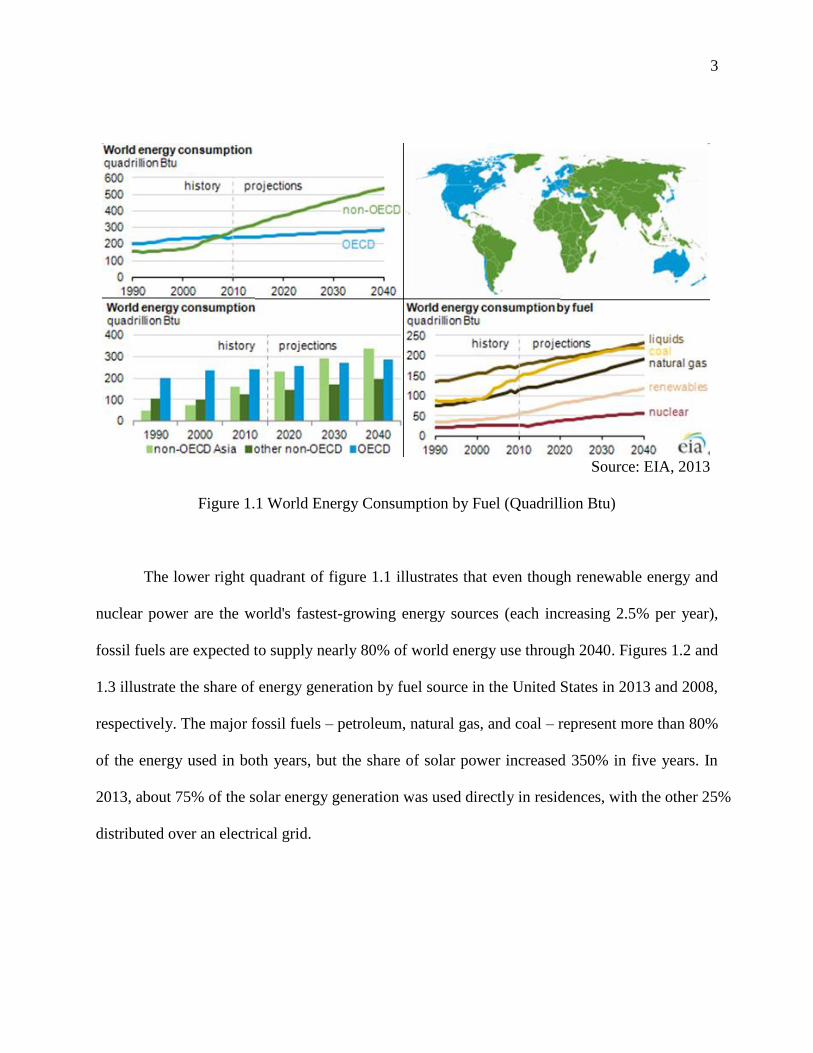
The U.S. Energy Information Administration (EIA) projects world energy consumption
will grow by 56% between 2010 and 2040, from 524 quadrillion British thermal units (Btu) to
820 quadrillion Btu by the OECD (Organization for Economic Cooperation and Development)
countries (Figure 1.1). Even though the OECD members (composed of 34 mostly developed
countries) will steadily increase energy use, most of this increase will come from non-OECD
countries, where demand is high due to strong economic growth and expanding populations
3
Source: EIA, 2013
Figure 1.1 World Energy Consumption by Fuel (Quadrillion Btu)
The lower right quadrant of figure 1.1 illustrates that even though renewable energy and
nuclear power are the world's fastest-growing energy sources (each increasing 2.5% per year),
fossil fuels are expected to supply nearly 80% of world energy use through 2040. Figures 1.2 and
1.3 illustrate the share of energy generation by fuel source in the United States in 2013 and 2008,
respectively. The major fossil fuels – petroleum, natural gas, and coal – represent more than 80%
of the energy used in both years, but the share of solar power increased 350% in five years. In
2013, about 75% of the solar energy generation was used directly in residences, with the other 25%
distributed over an electrical grid.

4
Source: Lawrence Livemore National Laboratory and EIA, 2014
Figure 1.2 Estimated U.S. Energy Use in 2013

5
Source: Lawrence Livemore National Laboratory and EIA, 2014
Figure 1.3 Estimated U.S. Energy Use in 2008

6
Since its inception, the Earth’s natural climate has oscillated between warm periods and
ice ages. Most often, the global climate has changed because of variations in the sun where the
amount of solar energy reaching the Earth has alternately increased and decreased (Riebeek,
2010). Since 1990, the IPCC offered its strongest language yet that Earth's climate is warming
and humans are largely responsible. According to Intergovernmental Panel on Climate Change
(IPCC), climate change refers to a change in the state of the climate that can be identified (e.g.
using statistical tests) by changes in the mean and/or the variability of its properties, and that
persists for an extended period. It refers to any change in climate over time, whether due to
natural variability or as a result of human activity.
Warming of the climate system is unequivocal, as is now evident from observations of
increases in global average air and ocean temperatures, widespread melting of snow and ice and
rising global average sea level (Figure 1.4). Smoothed curves represent decadal averaged values
while circles show yearly values. The shaded areas are the uncertainty intervals estimated from a
comprehensive analysis of known uncertainties (a and b) and from the time series (c).
Temperatures are expected to continue to rise.

7
Source: IPCC 2007
Figure 1.4 Changes in Temperature, Sea Level, and Northern Hemisphere Snow Cover

8
Figure 1.5 shows the history of temperature stretching back more than 800,000
years. Earth has experienced climate change in the past without help from humanity. The
mainstream climate science community has provided a theory (a record of Earth’s past climates,
or “paleoclimates.”) through the ancient evidence left in tree rings, layers of ice in glaciers,
ocean sediments, coral reefs, and layers of sedimentary rocks. Using this ancient evidence, the
record depicts that the modern climatic warming is happening more quickly than past warming
cases. According to NASA, as the Earth moved out of ice ages over the past million years, the
global temperature rose a total of 4 to 7 degrees Celsius over about 5,000 years. However, in the
past century alone, the temperature has climbed 0.7 degrees Celsius, roughly ten times faster
than the average rate of ice-age-recovery warming.

9
Source: NASA 2010
Figure 1.5 World Paleoclimate Record
Importantly, Figure 1.5 shows that the earth experiences a natural climate cycle without
any human interference. A warming trend accelerated and enhanced by greenhouse gas
emissions from human activity is projected to add to the frequency and severity of extreme
weather events such as the risk of dangerous floods, droughts, wildfires, hurricanes, and
tornadoes (CCSP, 2008). Considerable disruptions of ecosystems and ecosystem services are
also expected to occur (Schneider et al., 2007).

10
Food security is met when ‘all people, at all times, have physical and economic access to
sufficient, safe, and nutritious food to meet their dietary needs and food preferences for an active
and healthy life’ (FAO, 2008). Under various sets of assumptions, the International Panel on
Climate Change (IPCC) has conducted numerous studies on impacts associated with global
average temperature change for water, ecosystems, food and health (IPCC, 2007). For instance,
rain- dependent agricultural production could be reduced globally by up to 50% where access to
food in African countries depending on water, sun, and temperature is projected to adversely
affect food security and exacerbate malnutrition. Also, the productivity of some important crops
is projected to decrease and livestock productivity to decline, with adverse consequences for
food security as well (IPCC, 2007).
Unfortunately, continued reliance on conventional energy fuels will exacerbate global
warming; there is an urgent need to embrace a new energy paradigm to change the trajectory of
global temperatures. Countries around the world are looking for alternatives such as solar energy,
wind, biomass & biogas energy, hydro power, geothermal energy, and off-shore wind, wave, and
tidal energy. As UN Secretary General Ban Ki-Moon noted, “There is no plan B for climate
action as there is no planet B.”
Every day humans generate greenhouse gases (GHGs) such as carbon dioxide (CO2),
methane (CH4), nitrous oxide (N2O), hydrogen fluoride carbon (HFCs), phosphorus fluoride
carbon (PFCs), sulfur hexafluoride (SF6), and chlorofluorocarbon (CFCs) that trap heat in an

11
earth’s atmosphere. Table 1.1, shows how emissions levels of important pollutants vary across
fossil fuels. In a more detail sense, figure 1.6 describes the greenhouse effect where some of the
infrared radiation passes through the atmosphere, but most is absorbed and re-emitted in all
directions by greenhouse gas molecules and clouds. The effect of this is to warm the Earth’s
surface.
Table 1.1
Fossil Fuel Emissions Levels
Pollutant Natural Gas Oil Coal
Carbon Dioxide 117,000 164,000 208,000
Carbon Monoxide 40 33 208
Nitrogen Oxide 92 448 457
Sulfur Dioxide 1 1,122 2,591
Particulates 7 84 2,744
Mercury 0.000 0.007 0.016
Unit: pounds per billion Btu of Energy Input
Source: EIA, 1998

12
Source: ENVIS, 2012
Figure 1.6 Greenhouse Effect & Global Warming
Figure 1.7 shows the trend of U.S greenhouse gas emissions by gas type between year
1990 and 2012. In 2012, U.S. greenhouse gas emissions totaled 6,526 million metric tons of
carbon dioxide equivalents. Greenhouse gas emissions in 2012 were 10 percent below 2005
levels as well.

13
Source: EPA, 2013
Figure 1.7 U.S Greenhouse Gas Emissions by Gas, 1990-2012
Renewable sources often have a host of social, environmental, and economic benefits
such as: (1) Most renewable energy sources produce little to no GHG emissions. (UCSUSA,
2013b). (2) Compared with fossil fuel technologies, which are typically mechanized and capital
intensive, the renewable energy industry is more labor-intensive. This means that, on average,
more jobs are created for each unit of electricity generated from renewable sources than from
fossil fuels (UCSUSA, 2013a).

14
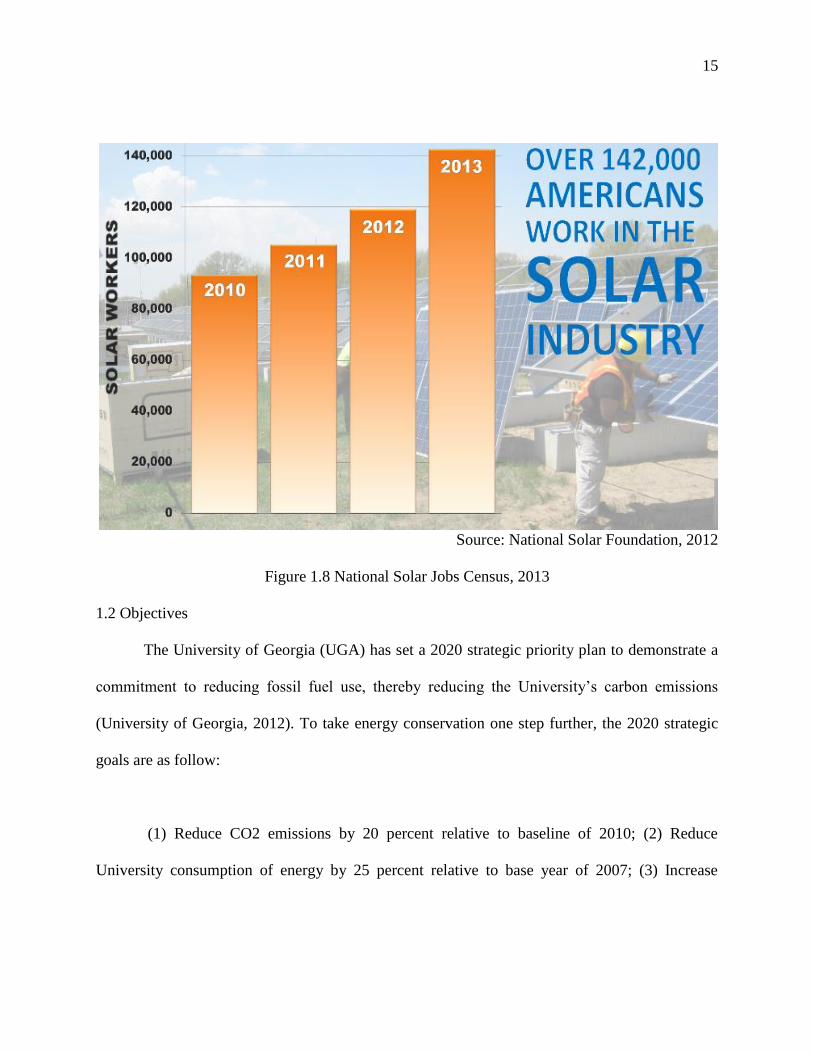
For example, in figure 1.8, the U.S. solar industry continues to grow at a faster pace than
the overall economy, supporting 142,698 jobs as of November 2013. Between September 2012
and November 2013, the solar industry added 23,682 jobs – an increase of 19.9 percent over the
Solar Foundation’s 2012 findings – approximately 10 times the national average job growth rate
of 1.9 percent (The Solar Foundation, 2011).
Also, according to Energy Future Coalition, the renewable energy technologies
developed and built in the United States are exported out of the country, helping to reduce the
U.S. trade deficit. Investments in energy efficiency upgrades to U.S. buildings could create
625,000 sustained jobs over the next decade. The American Council for an Energy-Efficient
Economy believes that every $1 invested in energy efficiency generates $3 in return-good for
businesses and consumers alike.
(3) Producing electricity from alternative energy rather than fossil fuels offers not only
significant public health benefits, but also environmental quality improvements. The air and
water pollution emitted by coal and natural gas plants is linked to breathing problems,
neurological damage, heart attacks, and cancer (Machol, 2013). Replacing fossil fuels with
renewable energy has been found to reduce premature mortality, lost workdays, and reduces
overall healthcare costs.
15
Source: National Solar Foundation, 2012
Figure 1.8 National Solar Jobs Census, 2013
1.2 Objectives
The University of Georgia (UGA) has set a 2020 strategic priority plan to demonstrate a
commitment to reducing fossil fuel use, thereby reducing the University’s carbon emissions
(University of Georgia, 2012). To take energy conservation one step further, the 2020 strategic
goals are as follow:
(1) Reduce CO2 emissions by 20 percent relative to baseline of 2010; (2) Reduce
University consumption of energy by 25 percent relative to base year of 2007; (3) Increase

16
purchase of energy from renewable sources by 10 percent with the baseline of 2010; (4) Increase
the generation of energy from renewable sources to 10 percent relative to baseline of 2010; (5)
build new construction on campus that targets a 20% reduction in energy consumption over
standard code compliance; and (6) integrate sustainability into both the undergraduate and
graduate student experience through curricular activities both in the classroom and beyond. Of
the six goals listed, this paper will focus on goals (1) and (4).
The main objective in this paper is to evaluate the net present value of installing a
photovoltaic (PV) system at the University of Georgia and to estimate the contribution such a
system would make toward meeting UGA’s CO2 emissions reduction target. While there are
many different types of renewable energy available, this paper analyzes three distinct PV panels
(mono-crystalline, poly-crystalline and thin-film) across three different solar tracking devices
(fixed, single axis tracking, and double axis tracking) in a given size of 10 acre (UGA owned
property). Both state and federal renewable energy programs are included in the analysis.
Specific objectives of the study are to:
Determine the degree to which a 10-acre, ground-installed PV system in Athens, GA,
will help meet all the energy related criteria listed in the UGA 2020 Strategic plan.
Identify key parameters and design features that determine whether the system has a
positive net present value over its lifetime.
Estimate the number of years it takes for the system to realize a positive net present
value under different parameterizations.
17
Determine whether it will be more cost-effective for UGA to use their own created
electricity or create positive financial returns on PV investment by selling it back to
Georgia Power.
1.3 Study Area
Sustainability is a growing area of interest for many universities across the United States
where they are rapidly discovering that environmental and business performance can be
intricately linked. Emerging climate change policies, volatile and upward trending energy prices,
universal pressure on businesses to reduce costs, and increased public and investor awareness of
environmental issues are all demanding prudent management of energy and materials use at the
organizational level.
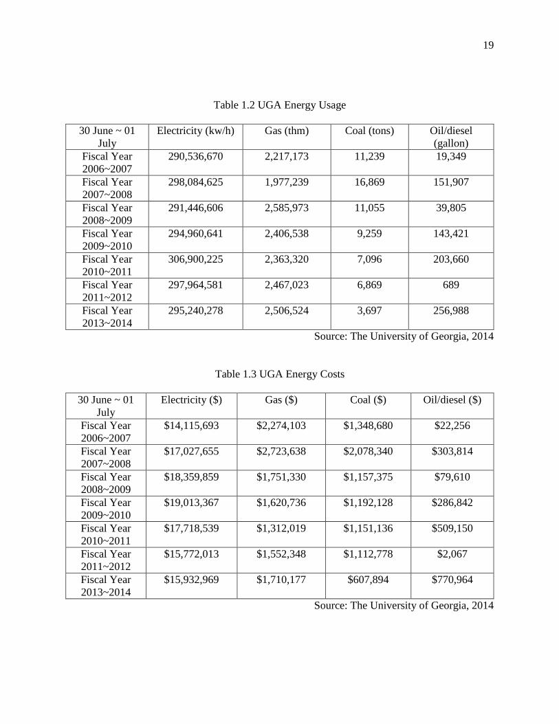
Under the fiscal year of July to June, both table 1.2 and figure 1.9 show the total energy
usage at UGA (2006~2014). Also, table 1.3and figure 1.10 explain the total energy cost at UGA
(2006~2014) as well. All of the natural gas, coal (bituminous) and Oil (Diesel) is used to only
generate heat for the buildings. As none of them were used to generate electric power, all the
electricity is bought from Georgia Power.
According to Georgia Power (2014), most of their electricity generation comes in the
order of coal (41%), Gas and oil (35%), Nuclear (22%), and Hydro (2%). While the graph for
the Energy Usage in UGA tends to be unstable due to the volatility of oil diesel price, the Energy

18
cost has remained constant, roughly around $14,000,000, despite the few ups and downs.
However, this paper will solely focus on the electricity usage and cost only.
19
Table 1.2 UGA Energy Usage
30 June ~ 01
July
Electricity (kw/h) Gas (thm) Coal (tons) Oil/diesel
(gallon)
Fiscal Year
2006~2007
290,536,670 2,217,173 11,239 19,349
Fiscal Year
2007~2008
298,084,625 1,977,239 16,869 151,907
Fiscal Year
2008~2009
291,446,606 2,585,973 11,055 39,805
Fiscal Year
2009~2010
294,960,641 2,406,538 9,259 143,421
Fiscal Year
2010~2011
306,900,225 2,363,320 7,096 203,660
Fiscal Year
2011~2012
297,964,581 2,467,023 6,869 689
Fiscal Year
2013~2014
295,240,278 2,506,524 3,697 256,988
Source: The University of Georgia, 2014
Table 1.3 UGA Energy Costs
30 June ~ 01
July
Electricity ($) Gas ($) Coal ($) Oil/diesel ($)
Fiscal Year
2006~2007
$14,115,693 $2,274,103 $1,348,680 $22,256
Fiscal Year
2007~2008
$17,027,655 $2,723,638 $2,078,340 $303,814
Fiscal Year
2008~2009
$18,359,859 $1,751,330 $1,157,375 $79,610
Fiscal Year
2009~2010
$19,013,367 $1,620,736 $1,192,128 $286,842
Fiscal Year
2010~2011
$17,718,539 $1,312,019 $1,151,136 $509,150
Fiscal Year
2011~2012
$15,772,013 $1,552,348 $1,112,778 $2,067
Fiscal Year
2013~2014
$15,932,969 $1,710,177 $607,894 $770,964
Source: The University of Georgia, 2014

20
Source: The University of Georgia, 2014
Figure 1.9 UGA Energy Usages
280,000,000
285,000,000
290,000,000
295,000,000
300,000,000
305,000,000
310,000,000
Ele
ctri
city
Usa
ge
(kw
/h)
Year
UGA Energy Usage
Electricity (kWh)

21
Source: The University of Georgia, 2014
Figure 1.10 UGA Energy Costs
$-
$2,000,000
$4,000,000
$6,000,000
$8,000,000
$10,000,000
$12,000,000
$14,000,000
$16,000,000
$18,000,000
$20,000,000
Co
sts
($)
Year
UGA Energy Cost (Athens, Georgia)
Electricity (kw/h)

22
Moreover, UGA’s s Sustainability and Architects for Facilities Planning Committee
commissioned a solar photovoltaic (PV) study to determine viable lands and buildings for the
installation of solar PV arrays. PV arrays can be mounted on the ground, rooftops or any other
suitable support structure. Figure 1.11 shows the map of Georgia highlighting Athens-Clarke
county. There are currently two areas that are identified by the UGA architecture as a potential
site for solar installations in terms of acreage and parcels. Those two areas are (1) Site A near the
intersection of Whitehall road and Phoenix road located in the south of Athens, (2) Site B near
the intersection of Lexington road and Old Lexington Road is located in the east of Athens.
From a bigger picture to smaller case, figure 1.12 shows more detailed locations of
Athens. Each parcel is 10 acres and they are as follow: Site A: 180 Hidden Hills Ln. Athens, GA
30605, and Site B: 6431-6463 Georgia 10. Winterville, GA 30683. They are currently owned by
UGA and are approved for building solar panels. However, in this paper we will consider only
site A because if the site is too far from the UGA campus, both the transmission loss and
equipment will result in higher costs when installing PV systems (Discussed further in chapter
5.3.3.5). Considering the main parts of a typical transmission and distribution network, the
overall losses between the generator and the consumers is about six percent (EIA, 2014).

23

24
Source: Arc GIS
Figure 1.11 Map of Athens, Georgia

25

26
Source: The University of Georgia
Figure 1.12 Capacity Potential for Installing Solar Panel at Site A and B

27
1.4 Organization
The rest of this paper is presented in the following order. The next three chapters are a
review about photovoltaic, U.S renewable energy policies, and an overview of electricity price
forecasting is discussed. Then, in the fifth and sixth chapter the feasibility of photovoltaic
installations and financial models are used in estimation to get the result. And finally,
conclusions have been presented.
28
CHAPTER 2
(ABOUT PHOTOVOLTAIC)
2.1 What is Photovoltaic System?
In 1839, a French physicist Alexandre E. Becquerel discovered that certain materials
would produce small amounts of electric current when exposed to light, also known as the
photovoltaic effect (Michael, 2008a). And it took more than a century before engineers would
develop photovoltaic (PV) cells that could change solar energy into electricity to run electrical
engines. Solar cells gained prominence in the 1970s when the energy crisis occurred to replace
fossil fuels. However, the prohibitive prices that is nearly 30 times higher than the year 2013
price made solar applications impractical and indifferent (Solar Energy Industries Association,
2014).
Wind energy already offers 2% of the world’s electricity, and their size is doubling
every three years (Carr, 2012). If that growth rate is sustained, wind farms will surpass nuclear
power plant impact to the world’s energy in about a decade. But it is in the field of solar energy,
currently only a quarter of a percent of the planet’s electricity supply.
While the price of fossil fuels is becoming more expensive, the technology development
in renewable energy has been getting cheaper over the past three decades. In figure 2.1, the
average cost of crystalline silicon solar cell has decreased from $76.67/watt in 1977 to just
$0.74/watt in 2013 and forecasted to decrease by $0.36/watt by 2017 (Rinaldi, 2013). The reason

29
for the small increase between 2005 and 2008 was due to poly-silicon shortage. Since 1998,
reported PV system prices have fallen by 6-8% per year on average, and the modules used to
make solar-power plants now cost less than a dollar per watt of capacity.
The figure 2.2 also explains the median reported installed prices of residential and
commercial PV Systems over time. All methodologies show a downward trend in PV system
pricing. The reported pricing and modeled benchmarks historically had similar results as well in
estimated pricing. On average, solar power has improved 14% per year in terms of energy
production per dollar invested (Economists, 2013). In some regions, the cost of electricity from
large-scale solar is now lower than the cost of retail electricity.
Figure 2.3 compares the price history of solar energy to oil and natural gas. While the
electricity price from conventional energy remained flat in inflation adjusted terms, the cost of
electricity from solar is dropping fast, and is likely to continue as technology and manufacturing
processes improve (McConnell, 2013). The cost of solar is headed towards the wholesale cost of
electricity from natural gas and this could get utility companies and power plant developers to
switch to solar. This indicates that with careful financial planning for installing PV, residents can
cut electricity costs by putting solar panels on the roofs. In addition, major companies
like Walmart, IKEA, Google, Apple, Facebook, Costco, Kohl’s, Macy’s, Staples, and many
others are turning their eyes to solar (Cost of Solar, 2013).

30
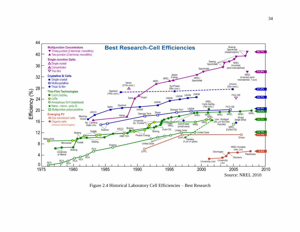
As indicated in Figure 2.4, solar cell efficiencies have increased at a steady rate over the
last several decades. Efficiencies for advanced multi-junction technologies have approached 40%
in laboratory settings at STC conditions. However, efficiencies for practical cells, such as
crystalline and thin film technologies, are well below these levels in the field.
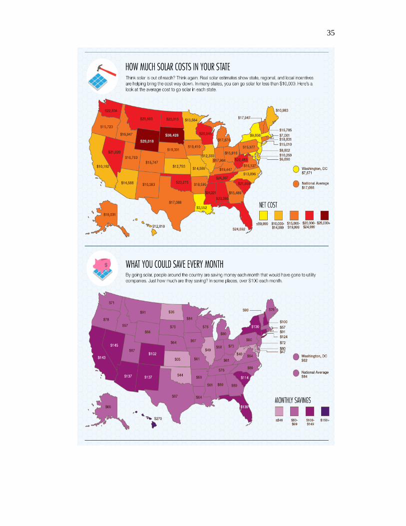
In figure 2.5, the energy analytics by Clean Power Research have used the results of 45,000 solar
estimates created by real U.S. homeowners in 2011 and placed them into maps to show how
much the solar system cost. And the maps are divided into four sections: (1) how much solar
costs in each state, (2) how much could be saved every month, (3) how much could be saved
over time, and (4) how long it will take to pay for itself after installing solar system.

31
Source: Bloomberg New Energy Finance (BNEF)
Figure 2.1 Solar Panel Prices Over Time (1977~2013)

32
Source: U.S. Department of Energy, 2014
Figure 2.2 Median Reported Installed Prices of PV Systems over Time

33
Source: Brian McConnell, Resilience
Figure 2.3 History of Solar Energy to Oil & Natural Gas
34
Source: NREL 2010
Figure 2.4 Historical Laboratory Cell Efficiencies – Best Research
35

36
Source: Clean Power Research, 2011
Figure 2.5 How Much Does Solar Cost?

37
2.2 Types of Solar Energy System
Before going into the different types of solar energy, the first way to look
at solar energy is by how it is converted into a useful energy. Passive solar
energy, facing the direction depending on hemisphere to provide natural lighting
and heating, is the harnessing of the sun’s energy without the use of mechanical
devices. On the other hand, active solar energy, which includes space (crystalline,
thin-film), water, and pool heating, uses mechanical devices in the collection,
storage, and distribution of solar energy to required areas (Michael, 2008b).
The second step is to look at the different types of solar energy. Solar
thermal energy is the energy created by converting solar energy into heat that is
put to practical use to heat water or space heating. Concentrating solar power is a
type of solar thermal energy that is aimed at large-scale energy production that
uses mirrors/lenses to concentrate sunlight to create high temperature to run
steam turbines/engines that eventually turns into electricity (Solar Energy
Industries Association, 2014). However, among the two major types of solar
power systems, this paper will solely focus on PV energy.
The name PV comes from the process of converting light (photons) to
electricity (voltage), which is known as PV effect (Engineering, 2013). PV cells
can be divided into either crystalline silicon PV which accounts for roughly 80%
of global PV production capacity or thin-film PV (a newer technology) which
accounts for 20% of global installed PV capacity (Business Insights, 2011).

38
Instead of using a traditional polycrystalline silicon, which is also known as
polysilicon (p-Si) and multi-crystalline silicon (mc-Si), thin-film cells use thin
layers of semiconductor materials like amorphous silicon (a-Si), copper indium
diselenide (CIS), copper indium gallium diselenide (CIGS), cadmium telluride
(CdTe) or organic photovoltaic cells (OPC).
So far, thin-film solar panels tend to take more space compared to
crystalline-based solar panels. On average, while thin-film cells convert 5~21%
of incoming sunlight into electricity, crystalline silicon cells can bring efficiency
of 11%~28% (NREL, 2012). However, there are still bright sides where thin-
film can increase more efficiency than crystalline silicon.
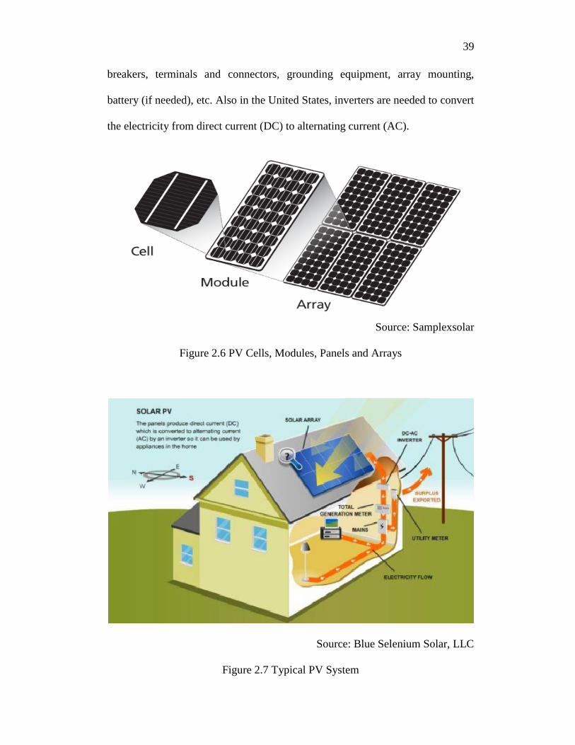
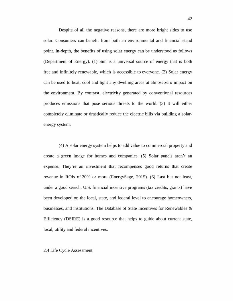
As shown in figure 2.6 and figure 2.7, a number of solar cells (about 40
cells) are connected to each other and mounted in a support structure or frame to
form a module. This PV module (panel) supports electricity at a certain voltage
(commonly 12 volts system) which is again wired together to form an array
(either in a fixed or tracking system) in both series and parallel electrical
arrangements. A typical home will use about 10 to 20 solar arrays to produce
direct-current (DC) electricity (NREL, 2014). And finally, both thin-film and
crystalline silicon systems use a variety of other components, known as
“balance-of-system (BOS)” components that include all mechanical or electrical
equipment and hardware: conductors and wiring methods, raceways and
conduits, junction and combiner boxes, disconnect switches, fuses and circuit
39
breakers, terminals and connectors, grounding equipment, array mounting,
battery (if needed), etc. Also in the United States, inverters are needed to convert
the electricity from direct current (DC) to alternating current (AC).
Source: Samplexsolar
Figure 2.6 PV Cells, Modules, Panels and Arrays
Source: Blue Selenium Solar, LLC
Figure 2.7 Typical PV System

40
2.3 Why Use Solar Energy?
To date, many natural resources have been applied with technology to
create and maximize a new market. Each year when summer arrive, the demand
for a chunk of electricity and water increase among agriculture, households,
industries, etc. For example, when constructing a hydroelectric dam, it stores lots
of water behind it in the reservoir. Then the water falls to spin a turbine and
create electricity to harness the energy potential.
As the sun’s radiant energy reaches every part of Earth’s surface,
installing solar panels on rooftops of buildings can provide electricity to even the
most remote locations. The potential of generating capacities vary from region to
region based on varying levels of solar radiation. Generating electricity with
photovoltaic and other renewable can reduce the amount of greenhouse gas
emissions from fossil fuel energy sources (Faiman, Raviv, and Rosenstrich,
2007).
Before examining the positive side of the solar system, it is also
important to take an honest look at the system’s disadvantages (Conserve-
energy-future, 2013). Some of the drawbacks are as follow: (1) The initial cost
of purchasing and installing solar panels always become the first disadvantage
when the subject is discussed. Even though subsidy programs, tax initiatives and
rebate incentives are provided by the government to promote the use of solar
panels, consumers are still hesitant to build PV system.

41
(2) The location of solar panels is important in the generation of
electricity. Areas such as U.K. that is mostly cloudy and foggy during day will
produce electricity at a reduced rate and may require more panels to generate
enough electricity. Moreover, solar panels that are covered by trees, landscapes
or other buildings are not appropriate to create electricity. (3) Most of the
photovoltaic panels are made up of silicon and other toxic metals like mercury,
lead and cadmium. Pollution in the environment can also degrade the quality and
efficiency of photovoltaic cells. However, new innovative technologies can
overcome the worst of these effects.
(4) Since not all the light from the sun is absorbed by the solar panels
therefore depending on the type of solar panels, the average efficiency rate of 20%
means that the rest of the 80% gets wasted and is not harnessed. However, the
endless R&D is slowly increasing the rate of efficiency of solar panels. (5) Solar
energy can only be harnessed when it is daytime and sunny. This means that
unlike other renewable source which can also be operated during night,
customers have to depend on the local utility grid to draw power in the night.
The consumer may consider using solar batteries to store excess power, however,
it is not recommended. (6) For home users, a large solar energy installation is not
required for huge space. But for big firms, a large area is required for the system
to be efficient in providing electricity.
42
Despite of all the negative reasons, there are more bright sides to use
solar. Consumers can benefit from both an environmental and financial stand
point. In-depth, the benefits of using solar energy can be understood as follows
(Department of Energy). (1) Sun is a universal source of energy that is both
free and infinitely renewable, which is accessible to everyone. (2) Solar energy
can be used to heat, cool and light any dwelling areas at almost zero impact on
the environment. By contrast, electricity generated by conventional resources
produces emissions that pose serious threats to the world. (3) It will either
completely eliminate or drastically reduce the electric bills via building a solar-
energy system.
(4) A solar energy system helps to add value to commercial property and
create a green image for homes and companies. (5) Solar panels aren’t an
expense. They’re an investment that recompenses good returns that create
revenue in ROIs of 20% or more (EnergySage, 2015). (6) Last but not least,
under a good search, U.S. financial incentive programs (tax credits, grants) have
been developed on the local, state, and federal level to encourage homeowners,
businesses, and institutions. The Database of State Incentives for Renewables &
Efficiency (DSIRE) is a good resource that helps to guide about current state,
local, utility and federal incentives.
2.4 Life Cycle Assessment

43
Life Cycle Assessment (LCA), also known as cradle-to-grave, is a
technique that studies the stages of raw material acquisition, materials
manufacture, production, use/reuse/maintenance, and waste management. The
system boundaries, assumptions, and conventions to be addressed in each stage
are presented. LCA is used as a decision-making processes - support tool for
both policy makers and industry in assessing the cradle-to-grave impacts of a
product or process (EPA, 2014). The following figure 2.8 is a simple picture of
LCA.
Source: The National Energy Technology Laboratory, 2014
Figure 2.8 LCA of Energy Technology and Pathways
Three forces are driving this evolution. First of all, the U.S. government
is putting a regulation that a manufacturer is responsible not only for direction
production impacts, but also for product inputs, use, transport, and disposal.
Secondly, business is participating in voluntary initiatives which contain LCA
and product stewardship components; for example, ISO to foster improvement
through better environmental management systems. Lastly, environmental

44
preferred has emerged as a criterion in both consumer markets and government
guidelines.
For three decades, hundreds of life cycle assessments have been studied
for residential and utility-scale solar systems. To further comprehend greenhouse
gas (GHG) emissions from commercial crystalline silicon (mono- and multi-
crystalline) and thin-film (amorphous silicon, cadmium telluride, and copper
indium gallium diselenide) PV power systems, the National Renewable Energy
Laboratory (NREL) LCA Harmonization Project was developed and applied a
systematic approach to review 400 published PV system studies, identify
primary sources of variability, and reduce variability in GHG emissions
estimates through a meta-analytical process called "harmonization" (NREL,
2013).
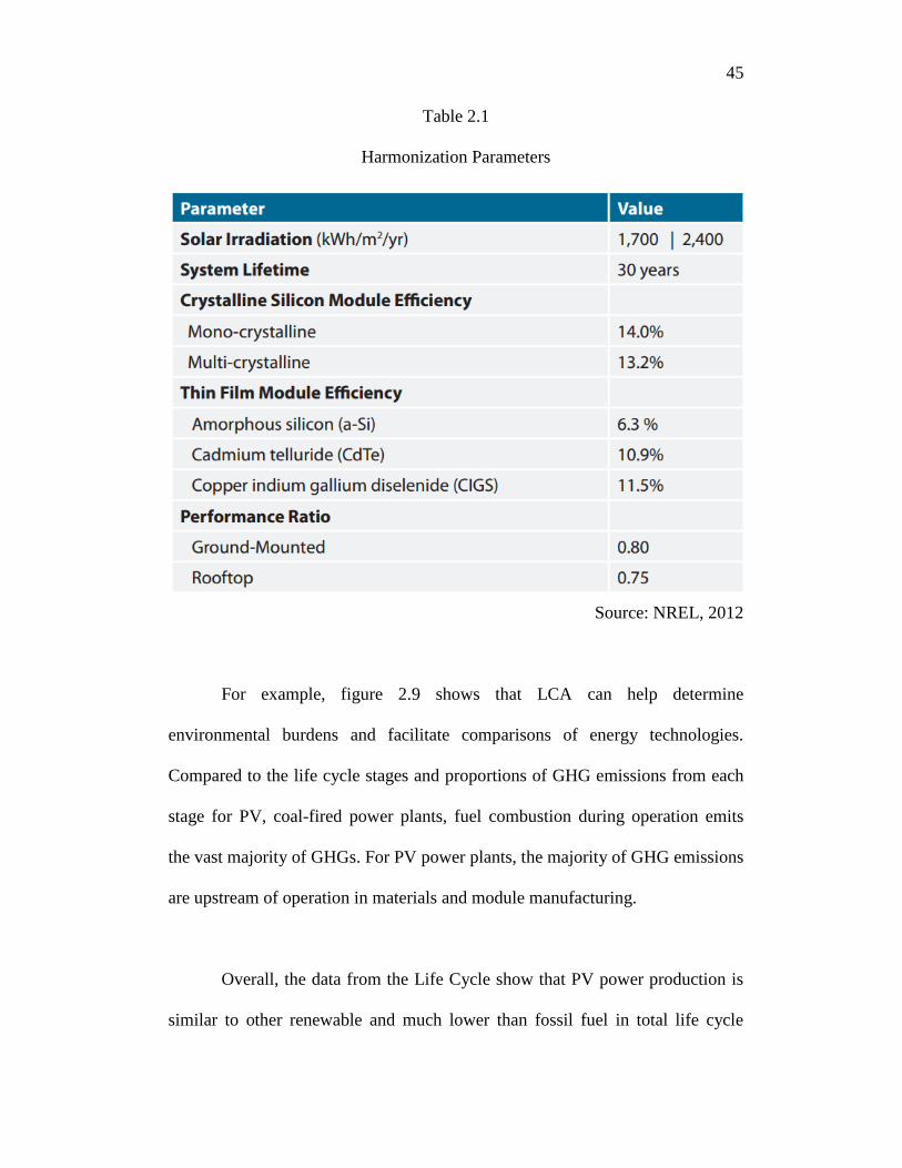
Table 2.1 shows the key technical parameters such as (1) Solar
irradiation, the average energy flux from the sun, in kilowatt-hours per square
meter per year, (2) Operating lifetime of the PV system and components, in
years, (3) Module efficiency, the percentage of the solar energy converted to
direct current electricity by the module, and (4) Performance ratio, the ratio of
alternating current electricity actually produced by the system, after accounting
for losses, to the electricity calculated based on the direct current-module
efficiency and irradiation.
45
Table 2.1
Harmonization Parameters
Source: NREL, 2012
For example, figure 2.9 shows that LCA can help determine
environmental burdens and facilitate comparisons of energy technologies.
Compared to the life cycle stages and proportions of GHG emissions from each
stage for PV, coal-fired power plants, fuel combustion during operation emits
the vast majority of GHGs. For PV power plants, the majority of GHG emissions
are upstream of operation in materials and module manufacturing.
Overall, the data from the Life Cycle show that PV power production is
similar to other renewable and much lower than fossil fuel in total life cycle

46
GHG emissions. Adjustment to a consistent operating lifetime is also a driving
factor in decreasing the variability of the harmonized data. Analysis between
mono-Si and multi-Si technologies suggests that these do not significantly differ
in life cycle GHG emissions. No significant differences in GHG emissions from
ground-mounted and roof-mounted systems were observed for c-Si or TF PV
technologies.
Source: Environmental Protection Agency, 2014
Figure 2.9 LCA Energy Systems

47
CHAPTER 3
(RENEWABLE ENERGY POLICIES)
3.1 U.S. Energy Agenda
The American Clean Energy and Security Act of 2009 (ACES), was
passed by the House of Representatives on June 26, 2009. This legislation
created a cap-and-trade mechanism, a market-based incentive to reduce carbon
emissions. It mandated a combined renewable electricity and energy efficiency
standard requiring that 20% of electricity sales by 2020 be met by renewable
energy and energy efficiency (ACEEE, 2013). In addition, allowances from the
trade of carbon credits in the cap-and-trade have offered funding for a number of
effective energy schemes. Together, these thoughts were able to support people
and business to benefit in the economy and enhance environmental quality.
The Feed-in Tariff (FIT) scheme is a government policy mechanism
designed to accelerate investment in renewable energy technologies such as low-
carbon electricity generation (EIA, 2013). FITs are used to a limited extent
around the United States, but they are more common internationally. A FIT
program guarantees customers who own a FIT-eligible renewable electricity
generation facility to receive a set price from their utility for all of the electricity
they generate and provide to the grid.
There are two main ways that the tariffs help the electricity producers to
make money via generating one’s own energy. The Generation and Export Tariff

48
where the producer earn a fixed income for every kilowatt hour of electricity the
producer generate via either using it for oneself or exporting it to the grid. Other
types of policies encouraging development of new renewable capacity that are
more commonly used in the United States is a Renewable Portfolio Standard
(RPS).
The RPS, also known as renewable electricity standard (RES), is a
regulatory mandate in the U.S. to catch three birds with one stone. (1) Save the
environment and reduce global warming, (2) Depend less of fossil fuels, and (3)
Increase the production of energy from renewable sources such as wind, solar,
biomass and other alternatives to fossil and nuclear electric generation (NREL,
2014). In recent years, many RPS proposals have been tried out through the U.S.
Congress; however, there is set standard program in place at the National level.
As shown in figure 3.1, each state have different policies to either require
(mandatory) or encourage (voluntary) electricity producers to supply a certain
minimum share of their electricity from chosen renewable energy resources by a
certain date/year.
These programs vary widely in terms of program structure, enforcement
mechanisms, size, and application. Other States also set goals for detailed types
of renewable energy or technologies to encourage growth. Currently every state
in the United States holds some type of financial programs for alternative energy
via availability of Federal tax incentives, State programs, and market conditions,

49
and as well as by State RPS policies. And most significantly, as with all
investments, one of the critical questions is whether polices for residential,
commercial, and utility scale solar installations will provide sufficient economic
returns to capital investments.
Source: Energy Information Administration, 2012
Figure 3.1 U.S. Renewable Portfolio Standards
RPS is most successful in stimulating alternative energy projects when
combined with federal investment tax credit (ITC). For example, the federal
government allows you to deduct 30% of your solar power system costs off
your federal taxes through an ITC (Solar City) before 31, 2016. After this
date, the commercial credit will drop to 10 percent and the residential credit
will drop to zero. Tax credits apply to certain actions such as purchasing an

50
energy-efficient vehicle or installing an eco-friendly home/firm; however, when
ITC have been withdrawn RPS alone can be ineffective (DSIRE, 2014 a1&a2).
In figure 3.2, the financial incentives for Solar PV tend to vary from tax
credit incentives, grants, loans, rebates, and performance based incentives for
individual and business investments. The Energy Department's Loan Program
guarantees loans to eligible clean energy projects with low interest rate and
provides direct loans to eligible manufacturers of advanced technology (Dept of
Energy, 2013). The Federal Grants are money that agriculture producers and
rural small business doesn’t have to repay and is based on one’s financial need.
They are also available for state government entities, local governments, tribal
governments, land-grant colleges and universities (DSIRE, 2014b). The 25
percent grant has been made possible through the USDA Rural Energy for
America (REPA) Grants program.

51
Source: DSIRE, 2009
Figure 3.2 U.S. Financial Incentives for Solar PV
Rebate is different from refunds where it gives back a portion of the
money taxpayers submitted earlier (ehow, 2010). The American Recovery and
Reinvestment Act of 2009 provides a renewable energy Production Tax Credit
(PTC) of $0.020 per kilowatt (kW) for the first 10 years or individuals who are
eligible for the PTC eligible for the U.S. Treasury investment tax credit (ITC)
(DSIRE, 2014c). The ITC equals to a 30 percent credit on all solar system
expenditures with no maximum credit (DSIRE, 2014c).
Gird parity happens when a renewable energy can generate electricity at
a levelized cost (LCoE) that is less than or equal to the price of purchasing
power from the electricity grid without subsidies or government support (REA).
In most countries (including the U.S.), solar system is currently just a small part

52
of the total energy production and consumption where PV remains a policy-
driven market. To become cost-competitive with other primary traditional
resources, solar energy must gain a larger share of the market via policy
incentives that decrease the overall costs to install solar panels and to put a high
pricing method for conventional electricity generation. Other renewable
resources, such as marine, geothermal and solar thermal, benefit from being
more controllable, but will make a smaller contribution than wind and solar due
to their higher costs and more limited resources (WEP, 2013).
Luckily, according to Lux research associate, “A 'golden age of gas' can
be a bridge to a renewable future as recent foundation of shale gas (year 2013)
will replace coal and act as a steppingstone until solar becomes cost-competitive
without subsidies with natural gas by 2025. In addition, in figure 3.3, it describes
that the cost per kilowatt hour of solar electricity has steadily declined from
nearly $5/kWh in 1978 to about $0.20 today, where the price of PV is projected
to become cost-competitive in the later future.

53
Source: MIT, 2009
Figure 3.3 Grid Parity
3.2 Renewable Policy Programs in Georgia
As of January 2012, 30 out of 50 U.S. states and the District of Columbia
have implemented mandatory Renewable Portfolio Standards (RPS) while seven
states have set voluntary goals for renewable generation (EIA, 2012).
Regulations vary from state to state and currently there is no RPS program in
place at the National level. The Georgia Chamber of Commerce does not support
any renewable portfolio program that has the ability to create an “economic
imbalance nationally, regionally or for Georgia” (Georgia Chamber of
Commerce). In other words, Georgia is not enrolled in either a standard or goal
for renewable energy. Therefore, in the state of Georgia, both individuals and
businesses can seek to voluntarily participate in renewable generation, especially

54
solar power system, from a combination of federal incentives, state programs,
and market conditions.
The incentives are as follow in the table 3.1: (1) Georgia Green Loans
Save and Sustain Program, (2) Federal Renewable Energy Tax Credit, and (3)
Solar Buyback Program from Georgia Power (DSIRE, 2014d).
Table 3.1
Available Incentives in Georgia
Name State Incentive
Type
Expiration
Date
Amount
Federal
Renewable
Tax Credit
Federal Residential,
Commercial,
Utility
~ Dec 31,
2016
30% of the costs
(installation)
Georgia
Clean
Energy Tax
Credit
State Residential,
Commercial,
Utility
~ Dec 31,
2014
$10,500 / $500,000 for
residential /
nonresidential
Georgia
Power –
Solar
Buyback
Local Residential,
Commercial,
Utility
$0.17 / kw/h
(X ≤100 kW)
$0.04 / kw/h
(100 kW <X≤ 80MW)
Source: DSIRE, 2014

55
3.3 About Georgia Power
The changing climate is affecting trends in weather across the nation. As
temperatures in the Southeast coast rise, humans will have to adjust to the
lengthening of cold seasons under extreme weather conditions. In 2011, Coal
accounted for 35 percent of Georgia Power's energy portfolio, Gas and Oil
generated 39 percent, Nuclear with 23 percent, and only three percent of the
consumed electricity was generated using hydro (Georgia Power Company,
2013). Every customer in Georgia is connected to the electrical grid where they
receive electricity from one of Georgia’s Public Service Commission (PSC)
approved utility providers. Georgia PSC tries to make sure that consumers
receive safe, reliable, and reasonable electricity price and natural gas price from
financially viable and technically experienced companies.
Currently, Georgia Power Company owns 18 generating plants and 20
hydroelectric dams across the state which provides electricity to 2.4 million
customers and consumers. Georgia Power is looking for improved ways to create
electricity and minimize environmental impact by investing $7 billion in
environmental control technologies until year 2015. However, Georgia Power
does not sell or recommend a specific system in regard to renewable energy.
Georgia Power is pushing for individuals and businesses to increase their
energy efficiencies to reduce the demand for electricity due to the likeliness of
power outage during peak consumption periods. Currently, they offer a

56
voluntarily solar buyback program for electricity generated through solar panels
that pays at a higher rate than standard net metering. Under the five year contract,
if the Georgia Power customers (commercial, residential, and industrial)
generate electricity they have the opportunity to sell some or all of the electricity
back to Georgia Power (DSIRE, 2014f). Small generators (X ≤ 100 kW) are
eligible to sell their electricity under the Renewable & Non-renewable Tariff
(RNR-8) at a rate equal to Georgia Power's avoided energy cost.
Georgia Power purchases energy from eligible providers on a first-come,
first-serve basis until the cumulative generating capacity of all renewable
sources reaches a specific amount set by the Georgia Public Service Commission.
The company will pay avoided energy cost as defined by the most recent
informational filing made by the company in compliance with the final order in
the PURPA Avoided Cost Docket 4822-U (Georgia Power Company, 2013).
Additional energy may be purchased by the company at a cost agreed to by it
and the Provider. Georgia Power will purchase energy from solar generating
facilities through the RNR tariff at the company's Solar Avoided Cost rate as
approved by the Georgia Public Service Commission.
Moreover, under the Solar Purchase Tariff (SP-2), customers can sell the
electricity that they have generated back to Georgia Power at a premium price,
currently 17.00 cents/kWh (Georgia Power Company, 2013). The amount of
capacity Georgia Power can contract for through the SP-2 Tariff is limited. This

57
limit is based on the amount of blocks of Premium Green Energy sold. And for
large customers (100 kW < X ≤ 80MW), they may sell their electricity as a
Qualifying Facility (Georgia Power), where the fixed price is at 4.00 cents/kWh.

58
CHAPTER 4
(LITERATURE REVIEW ON FORECASTING ELECTTRICITY PRICES)
4.1 U.S. Electricity Outlook
The price of electricity power generation depends largely on the type and
market price of the fuel, technology, government subsidies, government and
industry regulation, local weather patterns, and other factors. Moreover,
electricity rates not only differ at the state level, but also typically vary for
residential, commercial, and industrial customers. While the cost to generate
electricity changes minute-by-minute, most consumers end up paying rates based
on the seasonal cost of electricity (EIA, 2012). Electricity prices are highest in
the summer, and demand is usually highest in the afternoon and early evening
when usage is at a peak.
Both table 4.1 and figure 4.1 show the nominal average retail price of
electricity to ultimate customers by end-use in the state of Georgia. There are
four different electricity sectors (residential, commercial, industrial and
transportation) prices are normally higher for transportation, residential, and
commercial consumers than industrial consumers due to higher distribution costs.
The higher distribution costs stem from the fact that, those sectors generally use
less electricity and take their electricity at lower voltages it has to be stepped
down before it gets to the consumers (EIA, 2012). However, as UGA falls under
the commercial sector, we will focus on the latest commercial average electricity
price, 10.28cents per kWh ($0.1028 per kWh) in year 2014.

59
Table 4.1
Average Retail Price of Electricity to Ultimate Customers by End-Use Sector
Year Residential
(Cents /
kWh)
Commercial
(Cents / kWh)
Industrial
(Cents /
kWh)
Transportation
(Cents / kWh)
2014 11.57 10.28 6.52 6.31
2013 11.46 9.99 6.27 8.03
2012 11.17 9.58 5.98 7.65
2011 11.05 9.87 6.60 7.94
2010 10.07 9.06 6.22 7.46
2009 10.13 8.94 6.12 7.03
2008 9.93 9.07 6.67 7.15
2007 9.10 8.07 5.53 6.42
2006 8.91 7.81 5.38 6.12
2005 8.64 7.67 5.28 5.90
2004 7.86 6.88 4.43 5.12
2003 7.70 6.66 4.02 4.81
2002 7.63 6.46 3.95 N/A
2001 7.72 6.61 4.28 N/A
(In terms of nominal value)
Source: Environmental Protection Agency, 2015

60
Source: Environmental Protection Agency, 2015
Figure 4.1 Average Nominal Retail Price of Electricity, quarterly
4.2 Forecasting
The rapid increase in electricity demand over the last 100 years has
challenged both generating unit and system operators to build more nuclear
power plants, hydroelectricity dams, and small parts of systems related to
renewable energy to meet users’ supply. Because supply and demand for
electricity must balance in real-time, forecasting electricity demand is a critical
component of planning and operating electric generation and distribution. Based
on the needs of the market, a variety of approaches for forecasting electricity
price have been proposed in the last decades. Figure 4.2 shows the U.S.
Consumption for electricity generation (Btu) for electric utility, quarterly from
year 2000 to 2014.

61
Source: Energy Information Administration, 2015
Figure 4.2 Consumption for electricity generation (Btu) for electric utility,
quarterly
In contrast to other tradable commodities, electricity has two
characteristics (Eydeland and Wolyniec 2003; Kaminski 2013; Weron 2006).
First electric power cannot be stored economically. Second, power system
stability requires a constant balance between production and consumption. At
the same time, electricity demand depends on a variety of factors including the
weather (temperature, wind speed, precipitation, etc.) and the intensity of
business activities (working hours, weekdays vs. weekends, holidays and near-
holidays, etc.).
The characteristics of electricity loads can be seen in three ways: (1)
Time dependence, where electricity loads change according to the hour of the
day or time of year. For example, in terms of seasonality, every each year there

62
are two load peaks during summer and winter; (2) Regional dependence, where
during the same point in time across different locations, the electricity loads can
be dissimilar due to different consumption structures at each given region; and (3)
Temperature dependence, where different climate circumstances such as low or
high temperature affect electricity demand.
Electricity price can be forecasted in a variety of ways. One is the
interval estimate where one estimates prediction intervals (PI) via two averaging
schemes: simple average, and least absolute deviation (LAD). The second
method uses the concept of quintile regression and a pool of point forecasts of
individual time series models to construct prediction intervals. The latter can be
thought of an extension of LAD averaging. A lot of conventional ways such as
the AR(I)Max-GARCH model and the neural network model, have been used to
predict normal range electricity prices, however it ignores price spike measure
(Gaussian Mixture model, and K-NN model), which is caused by a number of
complex factors and exist during periods of market stress.
In the premature stage of data pre-processing, price spikes were truncated
before application of the forecasting model to decrease the influence of
observations on the estimation of the method parameters; otherwise a large
forecast error would be generated at price spike occasions (Yamin, 2004;
Rodriguez and Anders, 2004; Weron, 2006). In addition to understanding price
behavior, improved analysis of spikes is important for risk management as well.

63
On the other hand, the simple point estimates such as Artificial Neural
Network (ANN) can predict electricity price in nonlinear approximation via
direct forecasting method. Generalized regression neural network (GRNN) is
practical where it deals with few samples and sparse data in multidimensional
space. Recurrent neural networks (RNNs) are autoregressive nonlinear dynamic
models that show arbitrary nonlinear dynamic systems. Cross-validation is a
resampling technique that uses multiple training and test subsamples to avoid the
over fitting problem (Nima Amjady and Farshid Keynia, 2008). A result from
the cross-validation analysis provides valuable insights on the reliability or
robustness of neural networks with and is better than autoregressive (AR) error
models (Hsiao-Tien Pao, 2006).
The existed regression models are unable to cope with the nonlinear
relationships. Therefore, Artificial neural network (ANN) and support vector
machine (SVM) with nonlinear artificial intelligence forecasting methods been
suggested as the electricity loads are nonlinear. Besides in several engineering
problems, one-day ahead prediction using NN performed satisfactory outcome
(Chang et al. 2007). Pino et al. employed one-step ahead forecast method
(Enders 2004) within experimental procedure based on ANN with encouraging
outcome (Pino et al. 2008). Support Vector Machine (SVM) is an artificial
Intelligence Technologies based on statistical learning theory, which
approximates the relation curve by using only a small amount of training data.

64
Furthermore, SVM can effectively stay away from the over-fitting
problem by attaining an appropriate trade-off between empirical accuracy and
model complexity (Wen Yu, Haibo He, Nian Zhang, 2009); it shows better
performance compared to other traditional methods. Over-fitting is defined as
having too many parameters relative to the number of observations will normally
have bad predictive performance; particularly for noisy processes (Andreas S.
Weigend, Ashok N. Srivastava, Morgan Mageas, 1995).
On the other hand, relevance Vector Machine (RVM) is based on
Bayesian estimation theory, developed for regression and classification problems.
It can provide a solution function that depends on a very small number of
training samples, the relevance vectors (RVs). It shows better performance than
many other methods in terms of higher forecasting accuracy, model running time
(faster speed), and model complexity (Guoqiang Sun, Yue Chen, Zhinong Wei,
Xiaolu Li, and Kwok W. Cheung, 2014). However, the rules generated from
conventional statistical methods (i.e., ARIMA), and artificial intelligence
technologies (i.e., SVM and ANN) are not easily comprehensive for policy-
maker.
4.3 Types of Forecasting Method
The appropriate forecasting methods depend largely on what data are
available. The three factors for accurate forecasts needed are weather influence,
time factors, and customer classes. For weather influence, electric load has a

65
correlation to the weather where the important variables are dry and wet
temperature, dew point, humidity, wind speed and direction, sky cover, and
sunshine. The time factors such as the day of the week, the hour of the day and
holidays must be considered. In details, the three load forecast are short term
forecasts (one hour to a week), medium forecasts (a month up to a year), and
long term forecast (over one year). And finally, electric utilities serve different
types of customers such as residential, commercial, and industrial.
With all the considerations described above, electricity price forecasting
methods can be divided into five sections. The first group is the production-cost
(or cost-based) models which simulate the operation of generating units aiming
to satisfy demand at minimum costs (Wood, Wollenberg, 1996; Perez-Ruiz and
Conejo, 2000). It is the traditional engineering approach which ignores strategic
bidding practices (market power, gaming).
The second forecasting method is the equilibrium (or game theoretic)
approaches cost-based models with strategic bidding, agent-based models which
focus on the impact of bidder strategic behavior on electricity prices. It is said
that the spot market prices are closely related to the bidding and pricing
strategies of the market participants (Day, Hobbs and Pang, 2002, Green, 1992;
Smeers, 1997; Ventosa et al., 2005, Guan, 2001; Bajpai and Singh, 2004). It
poses problems if quantitative conclusions have to be draw. The modeling risk

66
associates the players, their potential strategies, the ways they interact and the set
of payoffs have to be defined.
Third is the fundamental (or structural) method which describes price
dynamics by modeling the impact of important physical and economic factors on
the price of electricity (Kanamura, 2006; Skantze, 2001; Vahvilainen, 2005). It
is better suited for medium-term rather than short-term price forecasting (STPF).
Fourthly, the artificial intelligence-based (or non-parametric) techniques
model price processes via non-parametric tools such as neural networks (NN),
fuzzy logic, etc. (Amjady, 2006; Gonzalez et al. 2005; Mandal et al. 2006;
Rodriguez, 2004). The method is flexible and can handle complexity and non-
linearity. However it is not intuitive and can perform below expectations.Neural
Network (NN) combines prediction from both Auto Regressive Moving Average
(ARMA) and GARCH models with historical price and demand data helps to
forecast a final normal range price.
Five short-term forecasting techniques were analyzed and evaluated by
Mogham and Rahman (1989), and autoregressive integrated moving averages
(ARIMA), forecasting homogeneous non-stationary performance was applied to
load forecasting (Hagan and Behr, 1987; Erdogdu, 2007). To overcome the
restrictions of linear models and to give a reason for nonlinear patterns, several
ways of nonlinear models have been proposed. These include threshold

67
autoregressive (TAR-type) models (Robinson, 2000) and an autoregressive
conditional heteroscedastic (ARCH) model of Engle (1982) and its extended
version GARCH, which simulates the heteroscedasticity of the residuals that
continues even after price spikes were gained from the original price time series,
(Bollerslew, 1986; Garcia, 2005; Jablonska, 2008). Also, ANNs have been
recommended as another way for time series predicting (Zhang 2005; Catalão,
2007).
Despite that both linear regression based models and ANNs models have
attained achievement in linear or nonlinear relationship, nothing suits all
situations as a universal model. Since it is hard to recognize the uniqueness of
the data in an actual problem, hybrid methodology that has both linear and
nonlinear modeling has been projected. A model combining a NN model with a
seasonal time series ARIMA model has been studied by Tseng and Yu (2002).
This model did better than ARIMA and ANN models in terms of precision. Wu
and Shahidehpour (2010) extended a hybrid model for day-ahead price
forecasting, composed of linear (ARMAX) and nonlinear (ANN) relationships of
prices and explanatory variables such as electricity demand.
And lastly, the fifth forecasting approach is the quantitative and statistics
(or stochastic, econometric, reduced-form) model which characterize the
statistical properties of electricity prices over time, with the ultimate objective of
derivatives evaluation and risk management (Bunn, 2004; Burger et al.2004;

68
Eydeland, 2003; Geman, 2006; Kaminski, 1999; Lucia, 2002; Weron, 2007). If
there are no data available or if the data available are not relevant to the forecasts,
then the qualitative and statistics (Q and S) forecasting methods are
recommended.
They are fulfilled when the numerical data about the past is accessible,
and it is rational to assume that some parts of the previous patterns are likely to
continue. Most Q and S forecasting problems use either time series data
(collected at regular intervals over time) or cross-sectional data (collected at a
single point in time). However, the main disadvantage comes from difficulties
involved in including physical characteristics of power systems.
The latter tries to predict the value of something we have not observed,
using the information on the cases that we have observed. It is used when the
variable to be forecast exhibits a relationship with one or more other predictor
variables. Under this model, any change in predictors will affect the output of
the system in a predictable way, assuming that the relationship does not change.
Models include regression models, additive models, and neural networks.
For the former (e.g.: ARMA(X), AR(X)-GARCH, (S)ARIMA,
(S)TAR(X), Markov regime-switching models), it is useful when we are
forecasting something that is changing over time (e.g., stock prices, sales figures,
profits). In other words, it uses data on the variable to forecast, and does not

69
attempt to find the reasons which affect its performance. Therefore it will look
for trend and seasonal patterns, but ignore all other information such as
marketing initiatives, competitor activity, and changes in economic conditions.
4.4 Data Mining and Combining Forecast Method
Data mining techniques for forecasting electricity price spikes were
extended by Lu (2005). Jablonska (2011) introduced spikes into diffusion
models by providing an idea of Poisson jump component plus time varying
parameters. Data mining techniques were applied to the spike forecasting
problem, and achieved hopeful results (Lu, 2005; Zhao, 2007a). These
approaches have revealed reliable forecasting accuracy and stoutness, even with
deficient information and noisy market data. Data mining technique based on
Bayesian idea did better than other alternative techniques (decision tree, neural
network, winnow, SVM and K-nearest neighboring) bearing in mind prediction
accuracy and decision benefits (Zhao, 2007b).
Combining forecasts, sometimes referred to as composite forecasts, can
reduce errors arising from faulty assumptions, bias, or mistakes in data. The idea
of combining forecasts goes back to the late 1960s, giving credits to Bates and
Granger (1969) and Crane and Crotty (1967). Since then, many authors have
recommended the better performance of forecast combinations over the use of
individual models: see e.g. Clemen (1989), de Menezes et al. (2000),
Timmermann (2006).

70
Joining them is useful to the extent that they are used when there exists
(1) uncertainty as to the selection of the most accurate forecasting method, (2)
uncertainty associated with the forecasting situation, and (3) a high cost for large
forecast errors (Armstrong, 2001). In addition, the key principles for combining
forecasts are to use (1) different methods or data or both, (2) forecasts from at
least five methods when possible, (3) formal procedures for combining, (4)
$ equal weights when facing high uncertainty, (5) $ trimmed means, etc,
(Armstrong, 2001).
Some researchers object to the use of combining. Statisticians object
because combining brings disorder with traditional statistical procedures will
result in the calculations of statistical meaning. Others object because making a
comprehensive model that includes all of the related information might be more
effective; there is one right way to forecast. Despite the objections, the combined
forecast is never less accurate compared to the typical component forecast.
4.5 Conclusion
In conclusion, when predicting price movements each specific model
gives different forecast. However, it is not feasible to pick a single model to
make it the most reliable one. For instance, Aggarwal et al. (2009) compared
results from 47 publications and concluded: there is no systematic proof of one
model out performing over the other models. This fact is valuable information to
take into account that combining method for electricity price forecasts is crucial.

71
Recently, this approach has been carried out in the literature by Bordignon et al.
(2013), Nowotarski et al. (2014) and Raviv et al. (2013). All three cited papers
give analogous conclusions - they believe the advantage of merging can
forecasts for more accurate and point/range forecasts of electricity prices.
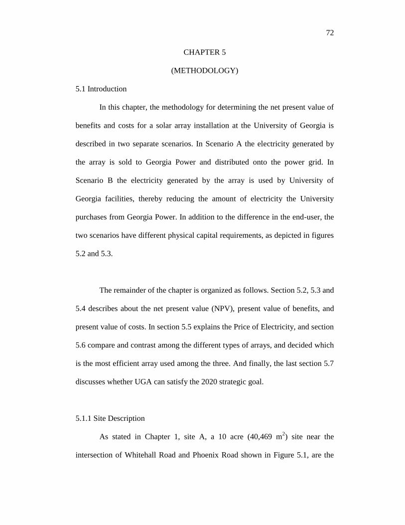
72
CHAPTER 5
(METHODOLOGY)
5.1 Introduction
In this chapter, the methodology for determining the net present value of
benefits and costs for a solar array installation at the University of Georgia is
described in two separate scenarios. In Scenario A the electricity generated by
the array is sold to Georgia Power and distributed onto the power grid. In
Scenario B the electricity generated by the array is used by University of
Georgia facilities, thereby reducing the amount of electricity the University
purchases from Georgia Power. In addition to the difference in the end-user, the
two scenarios have different physical capital requirements, as depicted in figures
5.2 and 5.3.
The remainder of the chapter is organized as follows. Section 5.2, 5.3 and
5.4 describes about the net present value (NPV), present value of benefits, and
present value of costs. In section 5.5 explains the Price of Electricity, and section
5.6 compare and contrast among the different types of arrays, and decided which
is the most efficient array used among the three. And finally, the last section 5.7
discusses whether UGA can satisfy the 2020 strategic goal.
5.1.1 Site Description
As stated in Chapter 1, site A, a 10 acre (40,469 m2) site near the
intersection of Whitehall Road and Phoenix Road shown in Figure 5.1, are the
73
possible study sites. Scenario A focuses on transferring the electricity to the
utility grid via Georgia Power Buy-Back Program, which requires a transformer
to transfer electricity to the utility grid via Georgia Power Buy-Back Program
with the transformer. And scenario B concentrates on distributing electricity to
UGA facilities such as the livestock arena and the UGA botanical garden, which
does not require a transformer and the electricity is directly used at UGA
facilities.
Source: Arc GIS
Figure 5.1 Capacity Potential for Installing Solar Panel at Site A
For easier view, we have drawn the system to get a rough estimate based
on the area available for the PV system. Figure 5.2 describes how the solar PV
system will be built in site A where no battery backup is necessary. In a given 10
acres, depending on the size of the module and array (acknowledging the space
between the arrays), we can fit multiple modules and arrays. Once all the arrays

74
are connected with the DC wire, we connect all the DC lines with the combiner
boxes in order to connect with the inverter and monitor.
Once the electricity is converted to AC power via the inverter, we
connect it to the main breaker and meters via AC wires. From this point on, the
difference is that while scenario A requires a transformer to connect to the grid,
scenario B does not require a transformer and is connected straight to the UGA
livestock and garden.
Source: Lim, 2015
Figure 5.2 Schematic of the System’s Physical Capital Requirements for
Scenario A and B

75
5.2. Net Present Value
Net Present Value (NPV) is often used in capital budgeting to analyze the
profitability of an investment or project; it is the difference between the present
value of cash inflows and the present value of cash outflows. The present value
of cash flows is computed by discounting them at the appropriate discount rate
(Weitzman, 1998).
The discount rate is the rate at which present and future cash flows are
traded off. It incorporates preference for current consumption, expected inflation,
uncertainty in future cash flows, and reduced liquidity via investing or loaning
out cash (Damodaran, 1996). The discount rate also represents the decision
maker’s patience – the lower the discount rate the more patient one is and vice-
versa.
As a general rule of thumb, a higher discount rate will lead to a lower
value for cash flows in the future. It is also an opportunity cost, since it captures
the returns that an individual would have on the next best opportunity. In a
discounted cash flow analysis, the sum of all net future cash flows
benefitst minus costst through the final period (T) is discounted back to the
present using a discount rate (r). In the analysis that follows the discount rate is
fixed at 4%. There is no particular set value; however, this is the lowest possible
discount rate at which projects are being financed in a solar market. The final
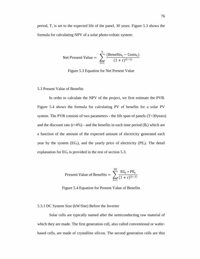
76
period, T, is set to the expected life of the panel, 30 years. Figure 5.3 shows the
formula for calculating NPV of a solar photo-voltaic system:
Net Present Value = ∑ (Benefitst − Costst)
(1 + r)(t−1)
T
t=1
Figure 5.3 Equation for Net Present Value
5.3 Present Value of Benefits
In order to calculate the NPV of the project, we first estimate the PVB.
Figure 5.4 shows the formula for calculating PV of benefits for a solar PV
system. The PVB consists of two parameters - the life span of panels (T=30years)
and the discount rate (r=4%) - and the benefits in each time period (Bt) which are
a function of the amount of the expected amount of electricity generated each
year by the system (EGt), and the yearly price of electricity (PEt). The detail
explanation for EGt is provided in the rest of section 5.3.
Present Value of Benefits = ∑EGt ∗ PEt
(1 + r)(t−1)
30
t=1
Figure 5.4 Equation for Present Value of Benefits
5.3.1 DC System Size (kW/Site) Before the Inverter
Solar cells are typically named after the semiconducting raw material of
which they are made. The first generation cell, also called conventional or wafer-
based cells, are made of crystalline silicon. The second generation cells are thin

77
film solar cells that are made of either amorphous silicon, CdTe, or CIGS cells.
For this paper, we decided to use three types of models (panels), (1) mono-
crystalline (c-Si), (2) poly-crystalline (poly-Si), and (3) thin-film (CdTe).
As shown in figure 5.5, each of the three modules are mounted on top of
the different types of array to calculate the DC system size before the inverter
(DCSSBIi,j, in terms of kW/site). DCSSBIi,j is the direct current power rating of
the photovoltaic array in kilowatts at standard test conditions (PVWatts,
2015). The DC system size before the inverter consists of module capacity (MCi,
in terms of kW), number of available modules per array (NAMAi,j), number of
available arrays with space per site (NAASSi,j), and array efficiency (AEj). And
among the three types of arrays used, we must first compare and contrast among
the different types of arrays to decide which is the most efficient array used
among the three.
DCSSBIi,j(kW/Site) = MCi ∗ NAMAi,j ∗ NAASSi,j ∗ AEj
Figure 5.5 Equation for DCSSBI
Moreover, the three module types (i) and three array types (j) are
evaluated in this study. The three tracking arrays evaluated in this study vary in
surface area and, therefore, vary in the number of modules a tracking array can
hold. It also follows that the number of tracking arrays that can be assembled

78
into a system on the site varies, based on the surface area of the array and the
movement of the tracking device.
5.3.1.1 Module (Panel) Types
In this section, we searched for companies that produce different types of
modules. And when considering three criteria such as durability (in years), price,
and amount of kW produced per panel, we chose Ben Q, Hanwha, and First
Solar because they are not only the top solar module manufacturers, but also has
high efficiency, in terms of product, with reasonable price. As shown in table 5.1,
it shows the technical specification of different solar modules (panels). The
Direct Current (DC) system size is the DC power rating of the photovoltaic array
in kilowatts (kW) at standard test conditions (STC). To calculate the Module
Generating Capacity (DC kW), it is equal to the Module Size (m²) × Efficiency
(%) × 1kW/ m²; Watts already include the module efficiency. However, this
fixed-tilt array area is the total module area, and does not include space between
the modules.

79
Table 5.1
Technical Specification of Different Solar Modules (Panels)
Product
Name
T1 T2 T3
Company Ben Q Hanwha FirstSolar
PV Cell
Type
Mono-crystalline Poly-crystalline Thin-film (CdTe)
Model PM250M01-260W HSL60P6-PA-4-
245TB
FS-390
# of
Available
Cells per
Module
60 60 154
Price $269 $230 $150
Efficienc
y
15.90% 14.8% 12.5%
Watts
(𝐒𝐓𝐂)𝐚
260W (0.26kW) 245W (0.245kW) 90W(0.090kW)
Initial
Cost
$1.04/Wdc $0.94/Wdc $1.67/Wdc
Module
(Panel)
Size
1.65m(L)×1.00m(W
) = 1.65m²
1.65m(L)×1.00m(W
)
= 1.65m²
1.20m(L)×0.60m(W
) = 0.72m²
Source for T1: Ecodirect, 2014
Source for T2: Hanwhasolarone, 2014
Source for T3: First solar, 2014
a: Average watts generated under Standard Test (STC) Conditions using a fixed
mounting
5.3.1.2 Array (Fixed, and Tracking) Types
Once we have found out the different types of panels to use, we would
need to find the most efficient array, in terms of high efficiency and low costs.
When comparing identical mounting system (either fixed or tracking), the
tracking-arrays will annually outperform the former in terms of energy
generation. As described in table 5.2 and figure 5.6, the annual improvement
between the two in the U.S can range from 0 to 40 percent depending on the

80
location and solar resource. There are four different types of mounting system
that brings different amount of efficiency and they are either fixed, single-axis,
two-axis. Commonly, except for the fixed, they all use motors to adjust the
array’s zenith, changing its angles to capture as much sun’s rays as possible all
year long (PVWatts NREL, 2014).
In a more detail sense, in table 5.2, the EmperySolar Company describes
that their tilted (Single-Axis) tracking array (TSTA) improves the efficiency by
average of 30% (between 25~35%) which would be equivalent to solar panels
with the average of 30% higher efficiency rating. Also, the BIG SUN Energy
Technology Company produces a universal (Two-Axis) tracking array (UDTA)
where the panels become average of 40% (between 35~45%) more efficient.
These two trackers create more efficiency because these devices change their
orientation throughout the day to follow the sun’s path to maximize energy
capture.
By virtue of having moving machinery, the tracking arrays always come
at an added cost relative to fixed-tilt arrays. The main drawbacks are as follow:
(1) Depending on the type of the array used, the motor in the device consumes
on average about 10% of the energy produced annually or simply between
10kWh and 15kWh per year (Easy Solar Poland, 2014; Big Sun Energy, 2015).
(2) As shown in table 5.18, the operations and maintenance costs (O&M) gets
higher in the order of fixed, single, and double. Also compared to mono and poly,

81
thin-film was $5 higher as well (Electric Power Research Institute, 2010). (3)
Due to the size of the array, installing the tracking-arrays increase land use and
land costs for the developer (PVWatts NREL, 2014).
As a whole, it is more cost-effective to install a fixed array for residential.
However, for commercial PV installations with an economy of scale that the
residential PV doesn’t have, it is better to use either single-axis or double-axis
tracking array (Kerr, 2013).
Source: Energy Information Administration, 2012
Figure 5.6 Fixed, Tilted, and Double Array Types

82
Table 5.2
Relative Average Generating Potential Across Array Systems
Array (Mounting) System Tilted Fixed Array (TFA) Tilted (Single-Axis) Tracking
Array (TSTA)
Universal (Two-Axis)
Tracking Array
(UDTA)
Company DPW Solar Inc. EmperySolar BIG SUN Energy
Technology Inc.
Array Type Standard Roof/Ground Mounts for
3 Type I
Tilt Single-Axis Tracking (EPR-
TSA)
TS-T6024AG (iPV)
Original Array Size
(Without Pole and space)
New Array Size
(With Pole and Space)
1.65m(L), 4.00m(W),
1.93m(H), 3.50m(B)
3.15m(L), 4.00m(W),
2.23m(H), 6.54m(B)
2.97m(L), 9.90m (W),
4.78m(H), 8.67m(B)
4.47m(L), 9.90m(W),
5.08m(H), 16.20m(B)
6.60m(L), 6.20m(W),
3.00m(H), 5.43m(B)
8.10m(L), 6.20m(W),
3.30m(H), 10.14m(B)
Array Tilt Angle (°)
(Oriented from South to North)
Tracking Range Angle(°)
(East to West)
Tracking Range Angle(°)
(South to North)
28.90°
Fixed
Fixed
28.90°
± 45°
Fixed
28.90°
± 45°
± 45°
Efficiency Factor 100 130 140
Array Power Consumption none 10 kWh/year 14kWh/year
Costs of Array $431 per TFA $1,404 per TSTA $3,120 per UDTA
83
Source for TFA: DPW, 2015; N. Arizona Wind & Sun, 2015
Source for TSTA: EmperySolar, 2013; Alibaba, 2013
Source for UDTA: BigSunEnergy, 2015, EnergyTrend, 2014

84
As shown in table 5.2, once we have chosen three types of arrays from
three different companies (DPW Solar, Empery Solar, and Big Sun Energy) we
can now estimate to see which is the most efficient with least costs array to use.
As similarly described in previous chapter 5.3.1.1, we have chosen three
different companies for the arrays because they are not only the top solar array
manufacturers, but also has high efficiency, in terms of product, with reasonable
price.
First of all, when designing a solar array shading is the enemy. Most
locations for solar projects tend to get around five to six net sun-hours per day,
so anything that obstructs that sunlight needs to be avoided at all costs. Shading
just one corner of a module can cut production in half, so avoiding shade on the
array is important (Reme). Therefore, rows and columns of solar panels need to
be optimally spaced to best use the available space.
The procedure for calculating shadow spacing starts with the altitude
angle of the installed array. For example, the city of Athens (Georgia) has the
latitude of 33.95°N, and longitude of 83.33°W (National Weather Service). And
if the latitude is between 25°N and 50°N, then the best tilt angles to use is to use
the latitude, times 0.76, plus 3.1 degrees. After careful calculation we get the
angle of 28.9°N, which is the optimum angle for the tilt array.
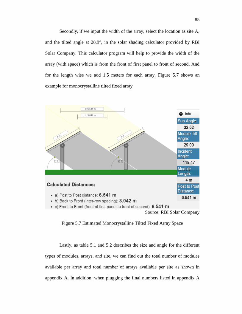
85
Secondly, if we input the width of the array, select the location as site A,
and the tilted angle at 28.9°, in the solar shading calculator provided by RBI
Solar Company. This calculator program will help to provide the width of the
array (with space) which is from the front of first panel to front of second. And
for the length wise we add 1.5 meters for each array. Figure 5.7 shows an
example for monocrystalline tilted fixed array.
Source: RBI Solar Company
Figure 5.7 Estimated Monocrystalline Tilted Fixed Array Space
Lastly, as table 5.1 and 5.2 describes the size and angle for the different
types of modules, arrays, and site, we can find out the total number of modules
available per array and total number of arrays available per site as shown in
appendix A. In addition, when plugging the final numbers listed in appendix A

86
to solve the equation in figure 5.5, we finally get table 5.3 which is equal to the
DC system size (kW/site) before installing the inverter.

87
Table 5.3
DC System Size Before the Inverter (kW per site)
Module
Capacity
(kW)
Total # of
Modules
Available
per Array
Total # of
Arrays
Available
per Site
Array
Efficiency
DCBI
(kW
per site)
T1-TFA
T2-TFA
T3-TFA
0.260
0.245
0.090
4
4
6
1,870
1,870
1,870
1.00
1.00
1.00
1,945
1,833
1,010
T1-TSTA
T2-TSTA
T3-TSTA
0.260
0.245
0.090
18
18
40
539
539
539
1.30
1.30
1.30
3,279
3,090
2,523
T1-UDTA
T2-UDTA
T3-UDTA
0.260
0.245
0.090
24
24
50
473
473
473
1.40
1.40
1.40
4,132
3,894
2,980
5.3.2 DC System Size (kW/Site) After the Inverter
PV arrays produce direct current (DC) from sunlight; and this DC current
is converted to alternating (AC) current with an inverter. This AC Power is then
used for operating all kinds of devices such as electric lights, kitchen appliances,
and air cone, or exporting it to the grid. As the inverters are not 100% efficient,
and energy is lost during this conversion process. A simplified schematic for a
residential PV installation is shown in figure 5.8.
Source: Homepower (2007)
Figure 5.8 Illustration of Grid-connected PV System
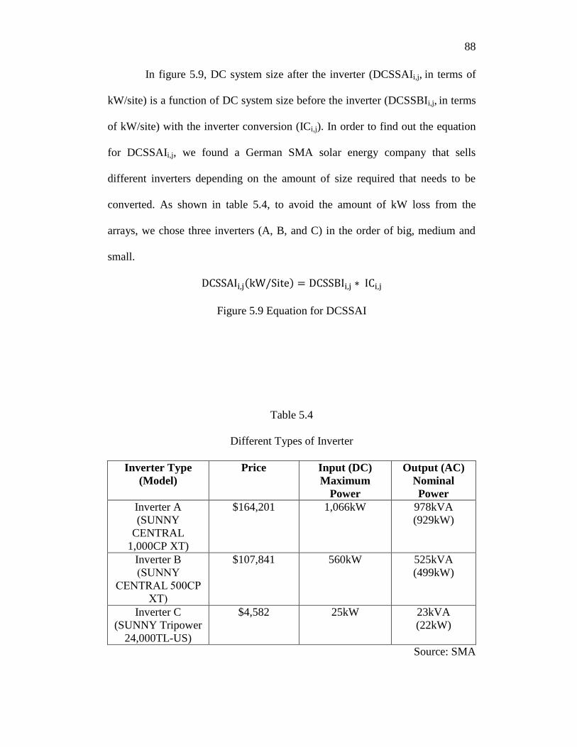
88
In figure 5.9, DC system size after the inverter (DCSSAIi,j, in terms of
kW/site) is a function of DC system size before the inverter (DCSSBIi,j, in terms
of kW/site) with the inverter conversion (ICi,j). In order to find out the equation
for DCSSAIi,j, we found a German SMA solar energy company that sells
different inverters depending on the amount of size required that needs to be
converted. As shown in table 5.4, to avoid the amount of kW loss from the
arrays, we chose three inverters (A, B, and C) in the order of big, medium and
small.
DCSSAIi,j(kW/Site) = DCSSBIi,j ∗ ICi,j
Figure 5.9 Equation for DCSSAI
Table 5.4
Different Types of Inverter
Inverter Type
(Model)
Price Input (DC)
Maximum
Power
Output (AC)
Nominal
Power
Inverter A
(SUNNY
CENTRAL
1,000CP XT)
$164,201 1,066kW 978kVA
(929kW)
Inverter B
(SUNNY
CENTRAL 500CP
XT)
$107,841 560kW 525kVA
(499kW)
Inverter C
(SUNNY Tripower
24,000TL-US)
$4,582 25kW 23kVA
(22kW)
Source: SMA
89
Since we have three different inverters, we first searched for an inverter
that is capable of holding the maximum input power for all types of arrays and
then converting it into AC. For example, one giant inverter A can hold input (DC)
maximum power of 1,066kW from table 5.4. This means that from the DCBIi,j of
1,945kW (T1-TFA) from table 5.3, we first divide it by 1,066kW/inverter to find
out that it can actually hold 1.82 inverters. However, as T1-TFA has a leftover of
0.82 (equivalent to 879kW) which is not fully converted by the giant inverter A,
we again use the medium size inverter B to divide 879kW by 560kW/inverter to
find out the number of inverters required.
Finally, since T1-TFA still has an excess of 319kW which is not
converted by the giant inverter B, we take the small size inverter C to divide
319kW by 24.5kW to get 13 inverters. Table 5.5 shows that when adding
inverter A, inverter B, and inverter C, T1- TFA creates a total of 1,683kW per
site. When comparing this number with 1,945kW per site from the previous
mentioned table 5.3, we can notice that about 15.54% of the electricity has been
lost during the conversion via inverter.

90
Table 5.5
DC System Size After the Inverter (kW per site)
Maximum Number
of Inverter A
Actual Number of
Inverter A
Leftovers from
Inverter A
Inverter A (kVA)
AC Output Power
Inverter A (kW)
DC Output Power
T1-TFA
T2-TFA
T3-TFA
1.82
1.72
0.95
1
1
0
878.800
766.600
1,009.800
978
978
978
929
929
929
T1-TSTA
T2-TSTA
T3-TSTA
3.08
2.90
2.37
3
2
2
81.276
958.087
390.520
978
978
978
929
929
929
T1-UDTA
T2-UDTA
T3-UDTA
3.88
3.65
2.80
3
3
2
934.128
695.736
847.900
978
978
978
929
929
929
Maximum Number
of Inverter B
Actual Number of
Inverter B
Leftovers from
Inverter B
Inverter B (kVA)
AC Output Power
Inverter B (kW)
DC Output Power
T1-TFA
T2-TFA
T3-TFA
1.569
1.369
1.803
1
1
1
318.800
206.600
449.800
525
525
525
499
499
499
T1-TSTA
T2-TSTA
T3-TSTA
0.145
1.711
0.697
0
1
0
81.276
398.087
390.520
525
525
525
499
499
499
T1-UDTA
T2-UDTA
T3-UDTA
1.668
1.242
1.514
1
1
1
374.128
135.736
287.900
525
525
525
499
499
499
Maximum Number Actual Number of Leftovers from Inverter C (kVA) Inverter C (kW)
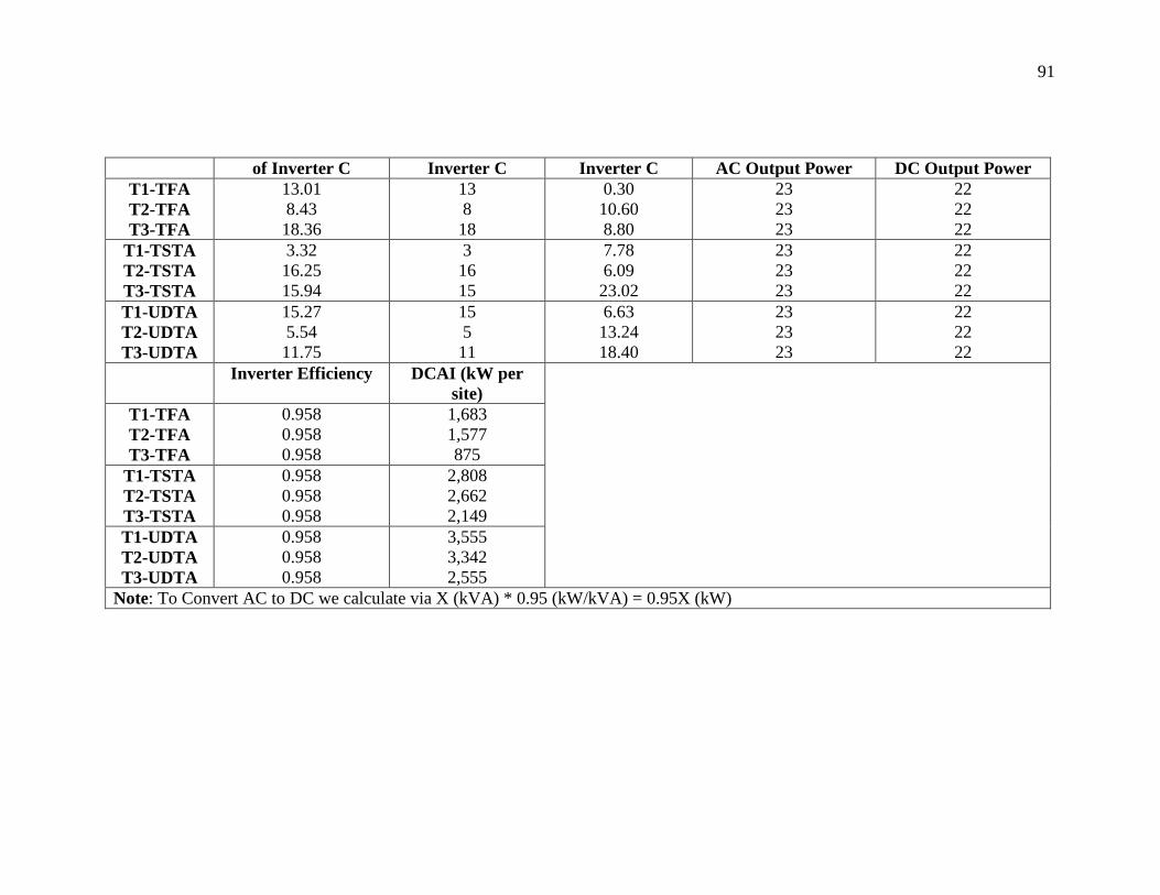
91
of Inverter C Inverter C Inverter C AC Output Power DC Output Power
T1-TFA
T2-TFA
T3-TFA
13.01
8.43
18.36
13
8
18
0.30
10.60
8.80
23
23
23
22
22
22
T1-TSTA
T2-TSTA
T3-TSTA
3.32
16.25
15.94
3
16
15
7.78
6.09
23.02
23
23
23
22
22
22
T1-UDTA
T2-UDTA
T3-UDTA
15.27
5.54
11.75
15
5
11
6.63
13.24
18.40
23
23
23
22
22
22
Inverter Efficiency DCAI (kW per
site)
T1-TFA
T2-TFA
T3-TFA
0.958
0.958
0.958
1,683
1,577
875
T1-TSTA
T2-TSTA
T3-TSTA
0.958
0.958
0.958
2,808
2,662
2,149
T1-UDTA
T2-UDTA
T3-UDTA
0.958
0.958
0.958
3,555
3,342
2,555
Note: To Convert AC to DC we calculate via X (kVA) * 0.95 (kW/kVA) = 0.95X (kW)

92
5.3.3 Expected Amount of Electricity Generated per Year (kWh/Site/Year)
In order to calculate the DC system capacity (kWh/Site/Year), we have
used solar radiation(kWh/m2/year), derate factor (system losses), efficiency
for different solar modules, 365 days per year, array power consumption and
step-up transformer (if needed) to solve the equation in figure 5.10. The
expected amount of electricity generated per year (EGt, in terms of
kWh/Site/Year) is itself a function of DC system size after the inverter
(DCSSAIi,j, in terms of kW/site), solar radiation (SRi,j, in terms of kWh/m2/
year ), derate factor (DRi,j), efficiency for different solar modules
(EDSMi,j), 365 days
1 year, array power consumption (APCi,j), and step-up transformer
(SUTi,j), if necessary. More details about each of the components are explained
below.
EGt = [(DCSSAIi,j ∗ SRi,j ∗ DRi,j ∗ EDSMi,j ∗ 365days) − APCi,j] − SUTi,j
Figure 5.10 Equation for EG
5.3.3.1 Solar Radiation Information
Solar Radiation (SR) is the amount of solar radiation energy received on
a given surface during a given time (PVWatts NREL, 2014). PV modules use the
light spectrum to generate electricity via the semiconductor material. Four
estimates of average daily solar radiation per month for the study area were
found in the literature (UGA Department of Geography, Synergy Environment
Engineers, NREL PVWatts1, and NREL PVWatts2). Each estimate used a

93
weighted average method that assigns a different weight to the global horizontal
irradiance, direct normal irradiance, temperature, wind speed, and other
meteorological data values to generate estimated of solar radiation (PVWatts
NREL, 2014).
Rather than picking just one estimate among the four, the average
monthly solar radiation of the four estimates was used to calculate the average
daily SR. Ideally it would be best to use a radiation for the next 30 years,
incorporating climate change projections. However, there is no future radiation
available at this point. Each month’s average SR was multiplied by the number
of days in the month, and summed across all months. The total was then divided
by 365.26 days to get the final average daily SR (kWh/m^2/day). For more
details, refer to table 5.6.

94
Table 5.6
Solar Radiation (Athens, GA)
Month SR1 SR2 SR3 SR4 Avg. SR
by
month
January 3.99 2.67 3.32 3.69 3.42
February 4.44 3.26 4.39 4.77 4.22
March 5.28 4.36 5.22 5.4 5.07
April 5.99 5.31 5.95 5.82 5.77
May 5.70 6.12 6.06 5.70 5.90
June 5.73 6.04 6.17 5.69 5.91
July 5.70 5.93 3.08 5.69 5.10
August 5.61 5.51 5.8 5.61 5.63
September 5.08 4.57 5.27 5.31 5.06
October 5.51 3.79 5.15 5.51 4.99
November 3.94 2.85 3.89 4.34 3.76
December 3.80 2.39 3.34 3.80 3.33
Average daily solar radiation 4.85
kWh/m^
2/day
Source for SR1: UGA Department of Geography, 2014
Source for SR2: Synergy Environment Engineers, 2014
Source for SR3: NREL PVWatts1, 2014
Source for SR4: NREL PVWatts2, 2014
95
5.3.3.2 Derate Factor (System Losses)
Inverters are just one source of power loss when converting from DC to
AC power. Therefore the inverter’s DC-to-AC conversion efficiency is a
separable input under the section 5.3.2. An example of other factors that
contribute to power losses in PV systems is shown in appendix B. The table
taken from NREL data used in the PVWATTS tool shows that there are
additional 11 factors that contribute to power losses.
There are many environmental factors that affect how much power a
system can produce. These include transformer and transmission line losses,
resistive factors, environmental conditions, and inverter losses. These factors are
combined for an estimated efficiency/derate value used in total system
generating size (PVWatts NREL, 2014). For the default values in the
PVWATTS tool, the forecast of overall derate factor is 0.77. In addition, as the
array efficiency is already included in the previous array section, we factor it out
in the derate factor.

96
5.3.3.3 Overall Solar Module Efficiency
Solar panel manufacturers put sufficient amount of effort into making
solar panels robust so that it can withstand heat/cold cycles and heavy weather.
In other words, this will help to reduce the expenses for the operations and
maintenance costs. However, solar panels are not perfect and they tend to
inevitably age. Table 5.7 illustrates the overall efficiency for different solar
modules where the solar system will wear down every year due to its ordinary
use and exposure.
The rated power output of solar system typically degrades at about 0.37%
per year. Polycrystalline silicon degrades the fastest among the thin-film solar
panels (CdTe) and monocrystalline silicon. The Pre and Post refer to
installations prior to and post 2000. In addition, if we are to apply table 5.7 to
our solar system, table 5.8 shows that monocrystalline still has higher efficiency
with the average of 96.70% during the 30 year period.
Table 5.7
Overall Efficiency for Different Solar Modules 1 (30 years)
Technology Output loss in percent / year
Pre Post
Amorphous silicon (a-Si) 1.30 0.95
Cadmium telluride (CdTe) 0.69 0.30
Copper indium gallium selenide
(CIGS)
3.50 0.02
Monocrystalline silicon (mono-Si) 0.90 0.23
Polycrystalline silicon (poly-Si) 0.60 0.59
Source: Jordan and Sarah, 2012

97
Table 5.8
Overall Efficiency for Different Solar Modules 2 (30 years)
Source: Jordan and Sarah, 2012
5.3.3.4 Array Power Consumption
As described in table 5.2, TFA uses zero power, TSTA with 10 kWh per
year, and UUDTA consumes 14kWh per year. And we plugged in the array
T1-All T2-All T3-All
Year 1 1.000 1.000 1.000
Year 2 0.998 0.994 0.997
Year 3 0.995 0.988 0.994
Year 4 0.993 0.982 0.991
Year 5 0.991 0.976 0.988
Year 6 0.989 0.971 0.985
Year 7 0.986 0.965 0.982
Year 8 0.984 0.959 0.979
Year 9 0.982 0.953 0.976
Year 10 0.979 0.947 0.973
Year 11 0.977 0.941 0.970
Year 12 0.975 0.935 0.967
Year 13 0.972 0.929 0.964
Year 14 0.970 0.923 0.961
Year 15 0.968 0.917 0.958
Year 16 0.966 0.912 0.955
Year 17 0.963 0.906 0.952
Year 18 0.961 0.900 0.949
Year 19 0.959 0.894 0.943
Year 20 0.956 03888 0.943
Year 21 0.954 0.882 0.940
Year 22 0.952 0.876 0.937
Year 23 0.949 0.870 0.934
Year 24 0.947 0.864 0.931
Year 25 0.945 0.858 0.928
Year 26 0.943 0.853 0.925
Year 27 0.940 0.847 0.922
Year 28 0.938 0.841 0.919
Year 29 0.936 0.835 0.916
Year 30 0.933 0.829 0.913
Average 0.967 0.914 0.957
98
power consumption in the equation of figure 5.10 to find out the expected
amount of electricity generated (kWh/Site/Year). Table 5.9 shows the expected
amount of electricity generated (kWh per Site per Year) which requires no
transformer. The electricity created from the PV system will be directly used for
UGA.

99
Table 5.9
Expected amount of electricity generated (kWh per Site per Year) – FOR UGA
DC System Size
After the Inverter
Solar Radiation
(kWh/m2/year)
Derate Factor Efficiency for Different
Solar Modules
Days/Year
T1-TFA
T2-TFA
T3-TFA
1,683
1,577
875
4.85
4.85
4.85
0.854
0.854
0.854
1
1
1
365
365
365
T1-TSTA
T2-TSTA
T3-TSTA
2,808
2,662
2,149
4.85
4.85
4.85
0.854
0.854
0.854
1
1
1
365
365
365
T1-UDTA
T2-UDTA
T3-UDTA
3,555
3,342
2,555
4.85
4.85
4.85
0.854
0.854
0.854
1
1
1
365
365
365
Array Power
Consumption
(kWh)
Step-up Transformer
(kWh)
Expected amount of
electricity generated
(kWh per Site per
Day)
Expected amount of
electricity generated
(kWh per Site per
Year)
Expected
amount of
electricity
generated
(mWh per
Site per
Year)
T1-TFA
T2-TFA
T3-TFA
Not Applicable
Not Applicable
Not Applicable
Not Applicable
Not Applicable
Not Applicable
6,969
6,528
3,623
2,543,720
2,382,578
1,322,536
2,544
2,383
1,323
T1-TSTA
T2-TSTA
10
10
Not Applicable
Not Applicable
11,617
11,011
4,240,013
4,019,081
4,240
4,019

100
T3-TSTA 10 Not Applicable 8,889 3,244,427 3,244
T1-UDTA
T2-UDTA
T3-UDTA
14
14
14
Not Applicable
Not Applicable
Not Applicable
14,706
13,823
10,566
5,367,718
5,045,435
3,856,479
5,368
5,045
3,857

101
5.3.3.5 Step-Up Transformer
Electricity has to be transmitted from large power plants to the
consumers via extensive networks. The transmission over long distances creates
power losses. The major part of the energy losses comes from joule effect in
transformers and power lines. The energy is lost as heat in the conductors.
Considering the main parts of a typical Transmission & Distribution network,
the average values of power losses at the different steps are as follow: (a) 1-
2% for step-up transformer from generator to transmission line, (b) 2-4% for
transmission line, (3) 1-2% for step-down transformer from transmission line to
distribution network, and (4) 4-6% for distribution network transformers and
cables (Schonek, 2013). The overall losses between the power plant and
consumers is then in the range between 8 and 15%.
However, among the different power losses at different stages, we will
only have to focus on step-up transformer and transmission line loss from PV
system to the utility grid. And the losses are between the range of one to six
percent, and we assumed the average of three percent for our analysis. In order
to calculate the transmission and transformer loss, we used appendix C to
calculate the SUTi,j loss. Table 5.10 shows the expected amount of electricity
generated (kWh per Site per Year) which requires transformer. The electricity
created from the PV system will be directly sold to Georgia Power.

102
Table 5.10
Expected amount of electricity generated (kWh per Site per Year) – TO SELL
DC System Size
After the Inverter
Solar Radiation
(kWh/m2/year)
Derate Factor Efficiency for
Different Solar
Modules
Days/Year
T1-TFA
T2-TFA
T3-TFA
1,683
1,577
875
4.85
4.85
4.85
0.854
0.854
0.854
1
1
1
365
365
365
T1-TSTA
T2-TSTA
T3-TSTA
2,808
2,662
2,149
4.85
4.85
4.85
0.854
0.854
0.854
1
1
1
365
365
365
T1-UDTA
T2-UDTA
T3-UDTA
3,555
3,342
2,555
4.85
4.85
4.85
0.854
0.854
0.854
1
1
1
365
365
365
Array Power
Consumption
(kWh)
Step-up
Transformer
(kWh)
Expected amount of
electricity generated
(kWh per Site per
Day)
Expected amount of
electricity generated
(kWh per Site per
Year)
Expected amount of
electricity generated
(mWh per Site per
Year)
T1-TFA
T2-TFA
T3-TFA
Not Applicable
Not Applicable
Not Applicable
209
196
109
6,760
6,332
3,515
2,467.408
2,311,101
1,282,860
2,467
2,311
1,283
T1-TSTA
T2-TSTA
T3-TSTA
10
10
10
349
331
267
11,268
10,681
8,622
4,112,703
3,898,399
3,146,985
4,113
3,898
3,147
T1-UDTA 14 442 5,206,533 5,206,533 5,207

103
T2-UDTA
T3-UDTA
14
14
415
317
4,893,919
3,740,631
4,893,919
3,740,631
4,894
3,741
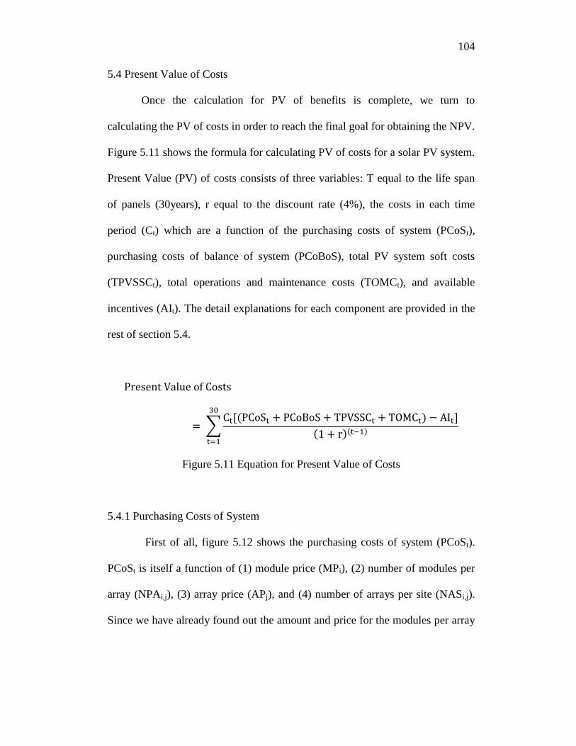
104
5.4 Present Value of Costs
Once the calculation for PV of benefits is complete, we turn to
calculating the PV of costs in order to reach the final goal for obtaining the NPV.
Figure 5.11 shows the formula for calculating PV of costs for a solar PV system.
Present Value (PV) of costs consists of three variables: T equal to the life span
of panels (30years), r equal to the discount rate (4%), the costs in each time
period (Ct) which are a function of the purchasing costs of system (PCoSt),
purchasing costs of balance of system (PCoBoS), total PV system soft costs
(TPVSSCt), total operations and maintenance costs (TOMCt), and available
incentives (AIt). The detail explanations for each component are provided in the
rest of section 5.4.
Present Value of Costs
= ∑Ct[(PCoSt + PCoBoS + TPVSSCt + TOMCt) − AIt]
(1 + r)(t−1)
30
t=1
Figure 5.11 Equation for Present Value of Costs
5.4.1 Purchasing Costs of System
First of all, figure 5.12 shows the purchasing costs of system (PCoSt).
PCoSt is itself a function of (1) module price (MPi), (2) number of modules per
array (NPAi,j), (3) array price (APj), and (4) number of arrays per site (NASi,j).
Since we have already found out the amount and price for the modules per array

105
and arrays per site required in table 5.3, we use this information to calculate the
purchasing costs for the systems in table 5.11.
Moreover, the three module types (i) and three array types (j) are
evaluated in this study. The three tracking arrays evaluated in this study vary in
surface area and, therefore, vary in the number of modules a tracking array can
hold. It also follows that the number of tracking arrays that can be assembled
into a system on the site varies, based on the surface area of the array and the
movement of the tracking device.
PCoSt = MP𝑖 ∗ NPA𝑖,𝑗 ∗ AP𝑗 ∗ NAS𝑖,𝑗
Figure 5.12 Equation for PCoS
Table 5.11
Purchasing Costs of System
Module
Price
($/unit)
Total # of
Modules
Available
per Array
Array
Price
($/unit)
Total # of
Arrays
Available
per Array
Total
Purchasing
Costs of
System
($/unit)
T1-TFA
T2-TFA
T3-TFA
$269
$230
$150
4
4
6
$431
$431
$431
1,870
1,870
1,870
$2,818,090
$2,526,370
$2,488,970
T1-
TSTA
T2-
TSTA
T3-
TSTA
$269
$230
$150
18
18
40
$1,404
$1,404
$1,404
539
539
539
$3,366,594
$2,988,216
$3,990,756
T1-
UDTA
$269
$230
24
24
$3,120
$3,120
473
473
$4,529,448
$4,086,720

106
T2-
UDTA
T3-
UDTA
$150 50 $3,120 473 $5,023,260
Note: System= Modules and Arrays
5.4.2 Purchasing Costs of Balance of System
Balance of system consists of transformer, monitor, meters, combiner
box, wiring, DC main breaker, AC main breaker, battery and inverter. For our
case we do not include the inverter because off-grid (with battery storage) is
mostly used when there is no grid access. In other words, it is best for a remote
area where the power lines don't reach, or when it is too expensive to extend
power lines to the desired location.
Moreover, the battery not only wastes 30% or more of solar power in
charging/discharging losses, throws away all excess solar power once batteries
are fully charged on an epic summer day, and requires high costs of O&M and
replacement fee, but also causes environmental harm due to lead, cadmium, and
mercury (Bob, 2011). Therefore, this paper will not consider off-grid system.
For more details in regard to battery waste, refer to figure 5.13.

107
Source: APRC, 2011
Figure 5.13 Off-Grid vs. Grid-Tie (Energy Loss)
Figure 5.10 shows the purchasing costs of balance of system (PCoBoS) is
a function of (1) derate factor costs (SLC), and (2) inverter costs (IC). In
appendix C, it describes both technical and price specification for the balance of
system. Also, we have already found out the amount and price for the inverters
in table 5.5. Therefore, by using this information, we calculate the number of
equipment required for each of the components in order to calculate the total
costs for the balance of system via figure 5.14. Table 5.12, table 5.13, table 5.14,
and table 5.15 shows the difference between not needing the step-up transformer
and requiring it. And it is easy to notice that the latter table has higher costs
compared to the former table because of requiring the extra step of installing the
step-up transformer.
PCoBoS = SLC + IC
Figure 5.14 Equation for PCoBoS
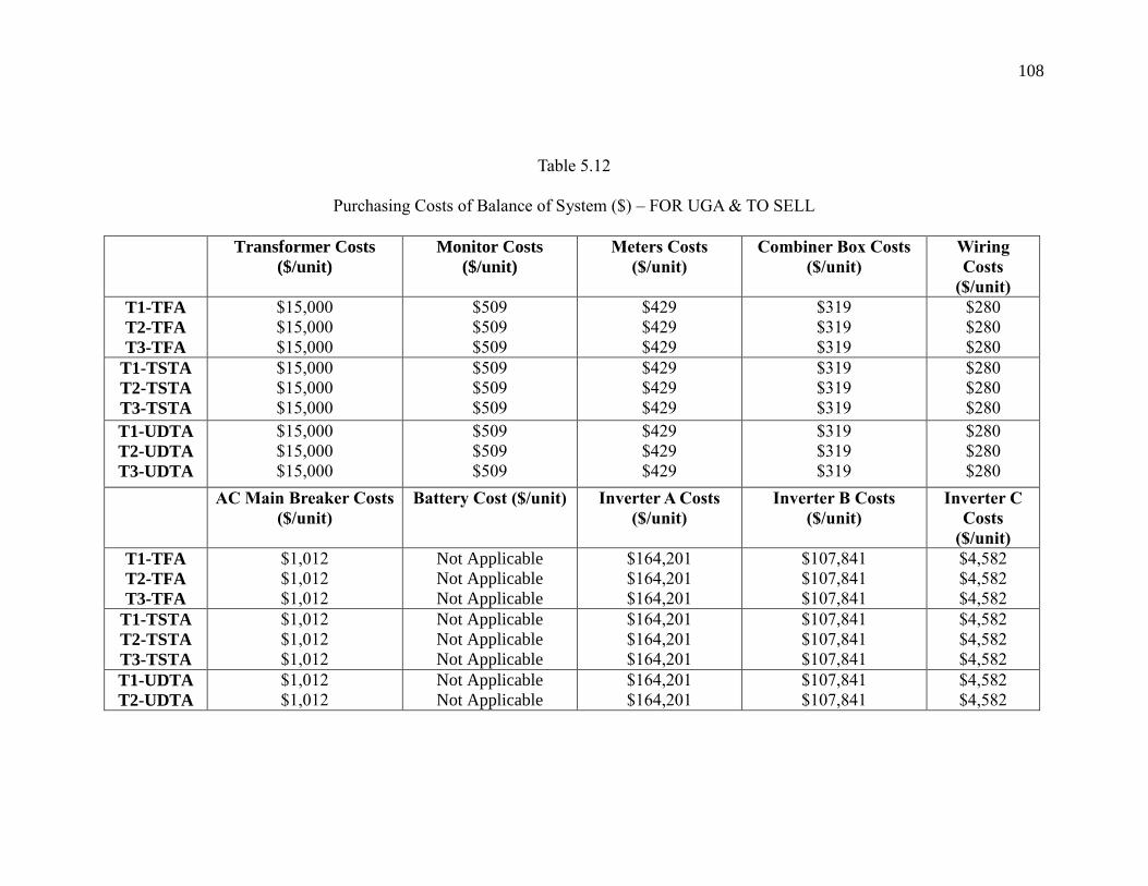
108
Table 5.12
Purchasing Costs of Balance of System ($) – FOR UGA & TO SELL
Transformer Costs
($/unit)
Monitor Costs
($/unit)
Meters Costs
($/unit)
Combiner Box Costs
($/unit)
Wiring
Costs
($/unit)
T1-TFA
T2-TFA
T3-TFA
$15,000
$15,000
$15,000
$509
$509
$509
$429
$429
$429
$319
$319
$319
$280
$280
$280
T1-TSTA
T2-TSTA
T3-TSTA
$15,000
$15,000
$15,000
$509
$509
$509
$429
$429
$429
$319
$319
$319
$280
$280
$280
T1-UDTA
T2-UDTA
T3-UDTA
$15,000
$15,000
$15,000
$509
$509
$509
$429
$429
$429
$319
$319
$319
$280
$280
$280
AC Main Breaker Costs
($/unit)
Battery Cost ($/unit) Inverter A Costs
($/unit)
Inverter B Costs
($/unit)
Inverter C
Costs
($/unit)
T1-TFA
T2-TFA
T3-TFA
$1,012
$1,012
$1,012
Not Applicable
Not Applicable
Not Applicable
$164,201
$164,201
$164,201
$107,841
$107,841
$107,841
$4,582
$4,582
$4,582
T1-TSTA
T2-TSTA
T3-TSTA
$1,012
$1,012
$1,012
Not Applicable
Not Applicable
Not Applicable
$164,201
$164,201
$164,201
$107,841
$107,841
$107,841
$4,582
$4,582
$4,582
T1-UDTA
T2-UDTA
$1,012
$1,012
Not Applicable
Not Applicable
$164,201
$164,201
$107,841
$107,841
$4,582
$4,582

109
T3-UDTA $1,012 Not Applicable $164,201 $107,841 $4,582
Note: Step-up Transformer (38,000kWh for DC System), Monitors (1,000kW for after inverter), Meters (12.5kW for after inverter),
Combiner Box (100kW for before inverter)
Table 5.13
Number of Balance of System – FOR UGA
# of Transformer
(38,000 kWh)
# of Monitors
(1,000kW)
# of Meters
(12.5kW)
# of Combiner Boxes
(100kW)
# of Wirings
(76.2m)
T1-TFA
T2-TFA
T3-TFA
Not Applicable
Not Applicable
Not Applicable
2
2
1
135
127
71
19
18
10
66
66
66
T1-TSTA
T2-TSTA
T3-TSTA
Not Applicable
Not Applicable
Not Applicable
3
3
2
225
213
172
33
31
25
66
66
66
T1-UDTA
T2-UDTA
T3-UDTA
Not Applicable
Not Applicable
Not Applicable
4
3
3
285
268
205
41
39
30
66
66
66
# of AC Main
Breakers
# of Battery # of Inverter A # of Inverter B # of Inverter C
T1-TFA
T2-TFA
T3-TFA
1
1
1
Not Applicable
Not Applicable
Not Applicable
1
1
0
1
1
1
13
8
18

110
T1-TSTA
T2-TSTA
T3-TSTA
1
1
1
Not Applicable
Not Applicable
Not Applicable
3
2
2
0
1
0
3
16
15
T1-UDTA
T2-UDTA
T3-UDTA
1
1
1
Not Applicable
Not Applicable
Not Applicable
3
3
2
1
1
1
15
5
11
Table 5.14
Number of Balance of System – TO SELL
# of Transformer
(38,000 kWh)
# of Monitors
(1,000kW)
# of Meters
(12.5kW)
# of Combiner Boxes
(100kW)
# of Wirings
(76.2m)
T1-TFA
T2-TFA
T3-TFA
1
1
1
2
2
1
135
127
71
19
18
10
66
66
66
T1-TSTA
T2-TSTA
T3-TSTA
1
1
1
3
3
2
225
213
172
33
31
25
66
66
66
T1-UDTA
T2-UDTA
T3-UDTA
1
1
1
4
3
3
285
268
205
41
39
30
66
66
66
# of AC Main
Breakers
# of Battery # of Inverter A # of Inverter B # of Inverter C

111
T1-TFA
T2-TFA
T3-TFA
1
1
1
Not Applicable
Not Applicable
Not Applicable
1
1
0
1
1
1
13
8
18
T1-TSTA
T2-TSTA
T3-TSTA
1
1
1
Not Applicable
Not Applicable
Not Applicable
3
2
2
0
1
0
3
16
15
T1-UDTA
T2-UDTA
T3-UDTA
1
1
1
Not Applicable
Not Applicable
Not Applicable
3
3
2
1
1
1
15
5
11
Table 5.15
Total Purchasing Costs of Balance of System ($) – TO SELL & FOR UGA
Total Purchasing Costs of BoS ($/unit) - TO SELL Total Purchasing Costs of BoS ($/unit) - FOR UGA
T1-TFA
T2-TFA
T3-TFA
$431,076
$404,323
$258,933
$425,849
$398,872
$221,408
T1-TSTA
T2-TSTA
T3-TSTA
$649,260
$646,638
$514,554
$710,440
$673,454
$543,767
T1-UDTA
T2-UDTA
T3-UDTA
$840,926
$786,945
$619,891
$899,476
$845,522
$646,477
112
5.4.3 Total PV System Soft Costs
According to the US Energy Department’s National Renewable Energy
Laboratory, soft cost is defined as financing and other non-hardware costs
(excluding the operations and maintenance). And the total PV system soft costs
(TPVSSCt) is a function of (1) customer acquisition costs (CACi,j), (2)
installation labor costs (ILCi,j), (3) permitting, inspection, and interconnection
costs (PIICi,j), and (4) labor for 3rd
party financing costs (L3PFCi,j). The detail
explanations for each component are provided in the rest of section 5.4.3.
TPVSSCt = CACi,j + ILCi,j + PIICi,j + L3PFCi,j
Figure 5.15 Equation for TPVSSC
As shown in figure 5.15, the benchmark 2010 soft cost includes areas of
(1) customer acquisition; (2) permitting, inspection, and interconnection (which
assumes the permitting fee); (3) installation labor; and (4) installer labor for
arranging third-party financing. Including assumed permitting fees, in 2010 the
average soft costs benchmarked in this analysis total $1.50/W for residential
systems (ranging from $0.66/W to $1.66/W).
First of all, customer-acquisition activities can add considerable time and
cost to PV installations, perhaps especially in states with less-mature markets
where perceived technology risk and unfamiliarity with PV might increase bid-
failure rates. Expenses related to customer acquisition—such as lead generation,

113
bid and pro-forma preparation, contract negotiation, and system design—
increase sunk costs to the installer.
Secondly, the installation labor cost is simply where electrician labor
comes in and helps to install the whole system size (PV, array, balance of system,
etc.).
Third, regulatory requirements and permitting processes for U.S. PV
installations are often burdensome and costly compared with those in leading PV
nations such as Germany (Langen 2010). Permitting, Inspection, and
Interconnection labor requirements includes the following elements: (1) Permit
Preparation—determination of a jurisdiction’s permitting requirements, travel
time to site, drawing of system plans, structural calculations, zoning application,
and delays; (2) Permit Package Submittal—travel time to and from the
permitting office and wait time at the permitting office;
(3) Permitting Inspection—paperwork, travel time to and from the site,
wait time for inspector, and physical inspection; (4) Interconnection Process—
paperwork, travel time to and from the site, wait time for representative from
utility, and physical interconnection; (5) Financial Incentive Application
Process—determination of eligibility, paperwork, travel time to and from the site,
wait time for inspector, and physical inspection.

114
Moreover, permitting and interconnection fees also significantly affect
total permitting costs. Total fees in the United States range from a low of $0 per
installation to an approximate high of $2,500 per installation (Vote Solar 2011,
Goodrich et al. 2012). For the purposes of this report, we assume a permitting
fee of $430 for a 5 kW residential system, or $0.09/W.
As with the residential survey results, the PII labor costs shown for
commercial PV do not include the cost of permitting or interconnection fees,
which may significantly surpass the direct PII labor costs. This report assumes a
$25,000 commercial PV systems permit fee, which equates to an additional
$0.35/W, in the median case, among survey respondents with average system
sizes smaller than 250 kW (assuming a system size of X>72 kW) and $0.03/W
among respondents with average system sizes larger than 250 kW (assuming a
system size of X>750 kW).
Lastly, as the upfront capital requirements of PV installations can deter
PV adoption, innovative third-party financing schemes that address these high
upfront requirements, such as solar leases and power purchase agreements
(PPAs) via financial analyst, are becoming more prevalent. For example, in 2010
approximately 33% of residential systems (by capacity) installed through the
California Solar Initiative used- third-party financing arrangements (California
Solar Statistics, 2012). And in 2011, this percentage grew to approximately 46%.

115
In table 5.16, the median 2010 benchmarked soft costs of commercial
systems are $0.99/W for systems smaller than 250 kW (ranging from $0.51/W to
$1.45/W) and $0.25/W for systems larger than 250 kW (ranging from $0.17/W
to $0.78/W). And when we use information to solve figure 5.15, we get the
calculation in table 5.17 which is the PV system soft costs for different types of
arrays.

116
Table 5.16
Summary of Commercial PV system Soft Costs in year 2010
Soft Cost Category
Residential Systems Small Commercial Systems
(<250 kW)
Large Commercial Systems
(> 205kW)
Cost ($/W) Proportion of
System Price
Cost ($/W) Proportion of
System Price
Cost ($/W) Proportion of
System Price
Customer Acquisition 0.67 10% 0.19 3% 0.03 1%
Installation Labor 0.59 9% 0.42 7% 0.18 3%
Permitting, Inspection,
and Interconnection
0.13 2% 0.02 0.3% 0.003 0%
Labor for Arranging 3rd
Party Financing
0.02 0.3% 0.02 0. 3% 0.01 0.2%
Assumed Permitting Fees 0.09 1% 0.35 6% 0.03 1%
All Surveyed Soft Costs 1.50 23% 0.99 17% 0.25 5%
Source: Ardani, Galen, Robert, Ryan, David, and Sean, 2012

117
Table 5.17
Total PV System Soft Costs ($)
Customer Acquisition
Costs ($)
Installation Labor
Costs ($)
PII Costs ($) Labor for 3rd Party
Financing Costs ($)
Total PV System
Soft Costs ($)
T1-TFA
T2-TFA
T3-TFA
$50,496
$47,297
$26,254
$302,976
$283,783
$157,527
$55,546
$52,027
$28,879
$16,832
$15,766
$8,751
$425,849
$398,872
$221,408
T1-TSTA
T2-TSTA
T3-TSTA
$84,242
$79.856
$64.478
$505,452
$479,137
$386,870
$92,666
$87,842
$70,926
$28,081
$26,619
$21,493
$710,440
$673,454
$543,767
T1-UDTA
T2-UDTA
T3-UDTA
$106,657
$100,260
$76,657
$639,944
$601,557
$459,944
$117,323
$110,286
$84,323
$35,552
$33,420
$25,552
$899,476
$845,522
$646,477
Note: Permitting, Inspection, and Interconnection (PII) Costs - includes assumed permitting fees, Labor for 3rd Party Financing
includes financial analyst

118
5.4.4 Total Opeartions and Maintenance Costs
Once UGA becomes an asset owner for PV system, however, will
demand that they need to consider operations and maintenance (O&M). Contrary
to popular belief, PV power plants are not maintenance free; they require a
regimen of continual monitoring, periodic inspection, scheduled preventive
maintenance, and service calls (Electric Power Research Institute, 2010). These
actions address unplanned outages, repair and restart, and various O&M
activities needed to enhance long term uptime, performance, and economic
viability.
Figure 5.16 offers a high-level percentage breakdown of total lifecycle
PV plant operations and maintenance costs for PV installation based on different
parts of the United States. Inverters are the most active component in a system,
are far and away the main culprit for unplanned PV plant downtime.
Miscellaneous site work represents the second largest expense; followed by BOS
upkeep, which tends to be the same across different arrays; and repair and
upkeep. Wiring issues are fairly minor and are minimized by preventative
maintenance practices. And modules, which have a less than 1% industry-wide
failure rate, require very little replacement.
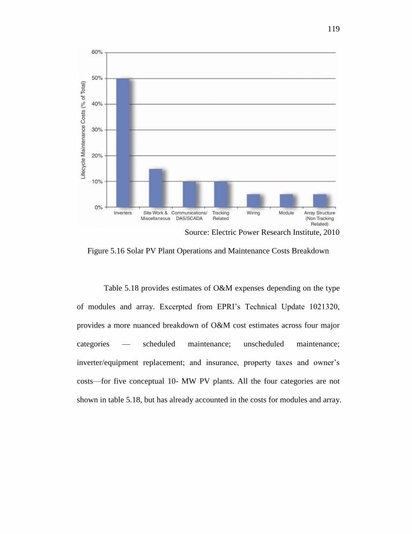
119
Source: Electric Power Research Institute, 2010
Figure 5.16 Solar PV Plant Operations and Maintenance Costs Breakdown
Table 5.18 provides estimates of O&M expenses depending on the type
of modules and array. Excerpted from EPRI’s Technical Update 1021320,
provides a more nuanced breakdown of O&M cost estimates across four major
categories — scheduled maintenance; unscheduled maintenance;
inverter/equipment replacement; and insurance, property taxes and owner’s
costs—for five conceptual 10- MW PV plants. All the four categories are not
shown in table 5.18, but has already accounted in the costs for modules and array.

120
Table 5.18
Total O&M Costs Estimates for Different Type of Modules and Array
Type of Modules and Array Total O&M Costs ($/kW/year)
Fixed-tilted monocrystalline $47/kW/year
Fixed -tilted polycrystalline $47/kW/year
Fixed -tilted thin-film (CdTe) $52/kW/year
Tilted single-axis monocrystalline $60/kW/year
Tilted single-axis polycrystalline $60/kW/year
Tilted single-axis thin-film (CdTe) $65/kW/year
Double-axis monocrystalline $73/kW/year
Double-axis polycrystalline $73/kW/year
Double-axis thin-film (CdTe) $78/kW/year
Source: Electric Power Research Institute, 2010
Scheduled Maintenance/Cleaning involves annual or biannual
preventative maintenance work and module cleaning, while Unscheduled
Maintenance comprises the costs to perform reactive repairs, such as handling
inverter problems and mechanical issues. Inverter Replacement Reserve
represents capital to refurbish all plant inverters near year 15. And Owner’s
Costs is composed of costs including monitoring, insurance, property taxes, site
communications and access, and other miscellaneous administrative fees and
expenses that the owner will incur. These are not costs that would be included in
a typical O&M contract, but are expenses that apply to all PV projects.
The total operations and maintenance costs (TOMCt) is a function of (1)
fixed operations and maintenance costs (FFOMCi,j), (2) scheduled maintenance
Costs (SMCi,j), (3) unscheduled maintenance costs (UMCi,j), (4)
inverter/equipment replacement costs (IERCi,j), and (5) insurance, property taxes
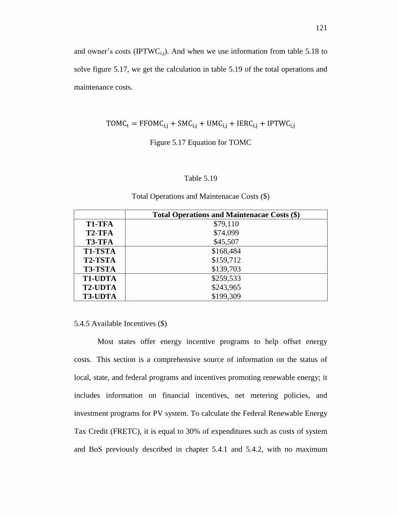
121
and owner’s costs (IPTWCi,j). And when we use information from table 5.18 to
solve figure 5.17, we get the calculation in table 5.19 of the total operations and
maintenance costs.
TOMCt = FFOMCi,j + SMCi,j + UMCi,j + IERCi,j + IPTWCi,j
Figure 5.17 Equation for TOMC
Table 5.19
Total Operations and Maintenacae Costs ($)
Total Operations and Maintenacae Costs ($)
T1-TFA
T2-TFA
T3-TFA
$79,110
$74,099
$45,507
T1-TSTA
T2-TSTA
T3-TSTA
$168,484
$159,712
$139,703
T1-UDTA
T2-UDTA
T3-UDTA
$259,533
$243,965
$199,309
5.4.5 Available Incentives ($)
Most states offer energy incentive programs to help offset energy
costs. This section is a comprehensive source of information on the status of
local, state, and federal programs and incentives promoting renewable energy; it
includes information on financial incentives, net metering policies, and
investment programs for PV system. To calculate the Federal Renewable Energy
Tax Credit (FRETC), it is equal to 30% of expenditures such as costs of system
and BoS previously described in chapter 5.4.1 and 5.4.2, with no maximum

122
credit (Department of Energy 1a). The FRETC is applicable for both personal
and business where the last date to apply is Dec 31, 2016.
As part of the Georgia Energy Challenge, Georgia offers tax credits for
certain types of energy efficient and renewable energy property. The applicable
energy sectors are either the lesser of 35 percent of the cost of the clean energy
property, or the sum of $10,500 for residential and $500,000 for nonresidential
per dwelling unit (Department of Energy 1b). And for the Georgia Clean Energy
Property Tax Credit (GCEPTC), the maximum incentive is $500,000 for UGA
PV system. It is also valid for both personal and business, however the last date
to apply was Dec 31, 2014.
And finally, the available incentives (AIt) is a function of (1) Federal
Energy Tax Credit (FETCi,j). Once satisfying figure 5.18, table 5.20 and table
5.21 shows the calculation for the total incentive benefits. And later we add total
incentive benefits to the total costs to reduce the total net costs.
AIt = FETCi,j
Figure 5.18 Equation for AI
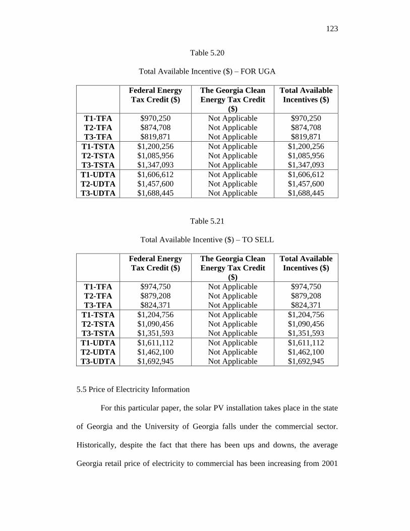
123
Table 5.20
Total Available Incentive ($) – FOR UGA
Federal Energy
Tax Credit ($)
The Georgia Clean
Energy Tax Credit
($)
Total Available
Incentives ($)
T1-TFA
T2-TFA
T3-TFA
$970,250
$874,708
$819,871
Not Applicable
Not Applicable
Not Applicable
$970,250
$874,708
$819,871
T1-TSTA
T2-TSTA
T3-TSTA
$1,200,256
$1,085,956
$1,347,093
Not Applicable
Not Applicable
Not Applicable
$1,200,256
$1,085,956
$1,347,093
T1-UDTA
T2-UDTA
T3-UDTA
$1,606,612
$1,457,600
$1,688,445
Not Applicable
Not Applicable
Not Applicable
$1,606,612
$1,457,600
$1,688,445
Table 5.21
Total Available Incentive ($) – TO SELL
Federal Energy
Tax Credit ($)
The Georgia Clean
Energy Tax Credit
($)
Total Available
Incentives ($)
T1-TFA
T2-TFA
T3-TFA
$974,750
$879,208
$824,371
Not Applicable
Not Applicable
Not Applicable
$974,750
$879,208
$824,371
T1-TSTA
T2-TSTA
T3-TSTA
$1,204,756
$1,090,456
$1,351,593
Not Applicable
Not Applicable
Not Applicable
$1,204,756
$1,090,456
$1,351,593
T1-UDTA
T2-UDTA
T3-UDTA
$1,611,112
$1,462,100
$1,692,945
Not Applicable
Not Applicable
Not Applicable
$1,611,112
$1,462,100
$1,692,945
5.5 Price of Electricity Information
For this particular paper, the solar PV installation takes place in the state
of Georgia and the University of Georgia falls under the commercial sector.
Historically, despite the fact that there has been ups and downs, the average
Georgia retail price of electricity to commercial has been increasing from 2001

124
(6.61cents/kWh) to 2014 (10.28cents/kWh). When referring back to table 5.22
the average retail price of electricity to commercial by end-use increased by
3.56%. Then, in order to forecast the electricity price, under the assumption
that the entire solar PV construction at UGA is built by the end of year 2015, we
had to project the average price of electricity for 30 year period from 2015 to
2044.
Undoubtedly, there are other factors that play a key role in affecting the
future electricity price such as fuels, power plants, transmission and distribution
system, weather conditions, policy (regulations), etc. However, to keep things
simple, we used the average increment (nominal growth rate) of 3.56% to
forecast the estimated electricity price for commercial by end-use from year
2015 to 2044. And in table 5.23, it was projected as 10.660cents/kWh in year
2015 and 30.387cents/kWh in year 2044.
On the other hand, due to the feed-in-tariff program utility companies are
required to buy electricity from qualified independent power producers since
1978 (Georgia Power, 2014). Georgia Power buys energy from solar resources
to supply the Green Energy Program through the Solar Purchase Tariff (SP-2).
Qualifying customers can sell all the energy produced from solar installations (X
≤ 100 kW in size) to GP at the Solar Purchase Price, currently 17 cents per kWh.
In addition, Georgia Power has a solar buyback program where the large

125
customers (X < 80 MW) can sell their solar generated back to GP as a
Qualifying Facility. According to Georgia Power, the current buyback
electricity price is fixed at 0.04cents/kWh for five-year period. This number may
increase or decrease in the next every five year period, however, there is no
estimated future electricity price over the 30 years. Therefore, we will use
0.04cents/kWh in this study.
Table 5.22
Average Retail Price of Electricity to Commercial by End-Use (Georgia)
Year Commercial (Cents /
kWh)
Nominal Growth Rate for
Commercial (%)
2014 10.28 2.903
2013 9.99 4.278
2012 9.58 (2.938)
2011 9.87 8.940
2010 9.06 1.342
2009 8.94 (1.433)
2008 9.07 12.392
2007 8.07 3.329
2006 7.81 1.825
2005 7.67 11.483
2004 6.88 3.303
2003 6.66 3.096
2002 6.46 (2.269)
2001 6.61 0
Average Nominal Growth Rate 3.56%
Source: EIA, 2012

126
Table 5.23
Estimated Future Average Retail Price of Electricity to Commercial by End-Use
(Georgia)
In terms of nominal value
Year Future Price (Cents / kWh) Year Future Price (Cents
/ kWh)
2044 30.387 2029 17.368
2043 29.343 2028 16.771
2042 28.335 2027 16.195
2041 27.361 2026 15.639
2040 26.421 2025 15.101
2039 25.513 2024 14.582
2038 24.637 2023 14.081
2037 23.790 2022 13.598
2036 22.973 2021 13.130
2035 22.184 2020 12.679
2034 21.421 2019 12.244
2033 19.975 2018 11.823
2032 19.289 2017 11.417
2031 18.626 2016 11.025
2030 17.986 2015 10.660
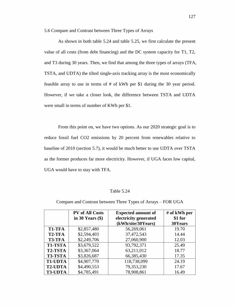
127
5.6 Compare and Contrast between Three Types of Arrays
As shown in both table 5.24 and table 5.25, we first calculate the present
value of all costs (from debt financing) and the DC system capacity for T1, T2,
and T3 during 30 years. Then, we find that among the three types of arrays (TFA,
TSTA, and UDTA) the tilted single-axis tracking array is the most economically
feasible array to use in terms of # of kWh per $1 during the 30 year period.
However, if we take a closer look, the difference between TSTA and UDTA
were small in terms of number of KWh per $1.
From this point on, we have two options. As our 2020 strategic goal is to
reduce fossil fuel CO2 emissions by 20 percent from renewables relative to
baseline of 2010 (section 5.7), it would be much better to use UDTA over TSTA
as the former produces far more electricity. However, if UGA faces low capital,
UGA would have to stay with TFA.
Table 5.24
Compare and Contrast between Three Types of Arrays – FOR UGA
PV of All Costs
in 30 Years ($)
Expected amount of
electricity generated
(kWh/site/30Years)
# of kWh per
$1 for
30Years
T1-TFA
T2-TFA
T3-TFA
$2,857,480
$2,594,403
$2,249,706
56,269,061
37,472,543
27,060,900
19.70
14.44
12.03
T1-TSTA
T2-TSTA
T3-TSTA
$3,679,522
$3,367,064
$3,826,687
93,792,371
63,211,012
66,385,430
25.49
18.77
17.35
T1-UDTA
T2-UDTA
T3-UDTA
$4,907,770
$4,490,553
$4,785,491
118,738,099
79,353,230
78,908,861
24.19
17.67
16.49

128
Table 5.25
Compare and Contrast between Three Types of Arrays – TO SELL
PV of All Costs
in 30 Years ($)
Expected amount of
electricity generated
(kWh/site/30Years)
# of kWh per
$1 for
30Years
T1-TFA
T2-TFA
T3-TFA
$2,868,316
$2,605,239
$2,260,542
54,580,990kWh
36,348,367kWh
26,249,073kWh
19.03
13.95
11.61
T1-TSTA
T2-TSTA
T3-TSTA
$3,690,022
$3,377,564
$3,837,187
90,976,178kWh
61,312,959kWh
64,391,627kWh
24.66
18.15
16.78
T1-UDTA
T2-UDTA
T3-UDTA
$4,918,270
$4,501,053
$4,795,991
115,172,565kWh
76,970,222kWh
76,538,458kWh
23.42
17.10
15.96
5.7 UGA 2020 Strategic Goal
As previously mentioned in chapter 1, the 2020 strategic objective was to
reduce fossil fuel CO2 emissions by 20 percent from renewables relative to
baseline of 2010. To answer goal one, we did the following order.
(1) In table 5.27, the amount of electricity which is first sold by Georgia
Power and then purchased by UGA in year 2010 is 294,961 mWh (294,960,641
kWh). (2) In table 5.26, the annual total output emission rates for greenhouse
gases (GHGs) is used as a default factor for estimating GHG emissions from
electricity use when developing a carbon footprint or emission inventory (EPA,
2014). Many of the boundaries shown on the map are approximate which is
provided by the North American Electric Reliability Corporation (NERC). And
under the different geographical boundaries shown, since the state of Georgia
falls under the Standards and Enforcement Review Committee (SERC)

129
Reliability Corporation/Central, we focus on 1,354 lbs of CO2/mWh, which is
the annual total output of carbon dioxide emissions.
As just mentioned above, we mutiply 294,961 mWh and 1,354 lbs of
CO2/mWh to get 399,403,254 lbs of CO2 produced. (3) In year 2016, which is
one full fiscal year, UGA has the capability to generate electricity for either
5,368 mWh (T1-UDTA TO sell), or 5,207 mWh (T1-UDTA FOR UGA) via PV
solar system. Then, in order to find out the amount of CO2 saved via UGA PV
generation, we multiply 5,368 mWh (to sell) by 1,354 lbs of CO2/mWh to get
7,268,376 lbs of CO2. And same thing applies for the No Transformer (for
UGA).
(4) In the end, for the No Transformer – for UGA, in order to calculate
the amount of CO2 reduced from renewables relative to baseline of 2010 in
terms of percentage, we calculated via [(7,268,376 lbs of CO2 divided it by
399,403,254 lbs of CO2) * 100] to get 1.82%. And for Yes Transformer– to sell,
same methods have been approached and resulted in 1.77%. Therefore, it shows
that the first goal can’t meet the criteria of 20%. Thinking on the positive side,
however, if we were to satisfy the goal for all 20%, we would require 11 more
lands (10 acres) that consist of PV generating system.
Moreover As shown in table 5.26, goal (4) from the 2020 UGA strategic
plan is to increase the generation of energy from renewable sources to 10 percent

130
relative to baseline of 2010. And after the same calculation as goal (1), we could
conclude that only 1.82% (For UGA) and 1.77% (To SELL) of solar energy
from renewable sources could be generated. In order to meet goal (4), we would
need at least six more sites, which is equivalent to 60 acres of land.

131
Table 5.26
Year 2010 GHG Annual Output Emission Rates by Company
NREC
acronym
Carbon Dioxide
(CO2) (lb/MWh)
Methane
(CH4) (lb/GWh)
Nitrous Oxide
(N2O)
(lb/GWh)
CAMX 610.82 28.49 6.03
FRCC 1196.71 38.91 13.75
SRSE 1354.09 22.82 20.89
SRVC 1073.65 21.69 17.64
U.S. Average 1,058.82 27.98 14.58
Source: EPA, 2014

132
Table 5.27
UGA Electricity Usage & CO2 Emission
UGA Energy Usage in year 2010
Fiscal Year 2009-2010 Electricity 294,961 mWh
GHG (CO2 Emission) Annual Output by Georgia Power in Year 2010
Fiscal Year 2009-2010 Emission 1,354 lbs of CO2/mWh
Total GHG (CO2 Emission) Annual Output by Georgia Power in Year
2010
Fiscal Year 2009-2010 Emission 399,403,254 lbs of
CO2
UGA PV Generation (2016)
Fiscal Year 2015-2016 For UGA (T1-UDTA) 5,368 mWh
Fiscal Year 2015-2016 To Sell (T1-UDTA) 5,207 mWh
GHG (CO2 Emission) Annual Output by Georgia Power in Year 2010
Fiscal Year 2009-2010 Emission 1,354 lbs of CO2/mWh
The Amount of CO2 Saved via UGA PV Generation (2016)
Fiscal Year 2015-2016 For UGA (T1-UDTA) 7,268,376 lbs of CO2
Fiscal Year 2015-2016 To Sell (T1-UDTA) 7,050,116 lbs of CO2
The Amount (%) of CO2 Reduced from Renewables Relative to Baseline
of 2010
Fiscal Year 2015-2016 For UGA (T1-UDTA) 1.82%
Fiscal Year 2015-2016 To Sell (T1-UDTA) 1.77%
The Increased Amount (%) of CO2 from Renewables Relative to Baseline
of 2010
Fiscal Year 2015-2016 For UGA (T1-UDTA) 1.82%
Fiscal Year 2015-2016 To Sell (T1-UDTA) 1.77%

133
CHAPTER 6
(RESULTS)
Given the model and the data outlined in the previous section, chapter 6
discusses the assessment of the economic feasibility of installing photovoltaic
systems for 30 years. The results for the UGA solar electricity generating
potential are based on the solar radiation, module, system size, array type,
system losses, available incentives (tax credit), and price of electricity. And for
the cost wise, it consists of total equipment costs, total installation, permit,
operations, and maintenance costs, etc.
There are two main end-use scenarios that are being examined to see
which is more financially beneficial. While scenario A (requiring the
transformer) discusses about selling the electricity generated from their solar
power to the utility company, scenario B (requiring no transformer) explains the
benefit of using their own electricity generation from UGA’s PV system. In
order to get the net present value (NPV) for both scenario A and B, we have
subtracted the PV of costs from the PV of benefits. In addition, among the three
types of tracking system, we have decided to use the universal double-axis
tracking array (UDTA) as discussed previously in chapter 5.
Table 6.1 and 6.2 describes the total expected amount of electricity
generation in each module for T1-UDTA (Mono-crystalline), T2-UDTA (Poly-
crystalline), and T3-UDTA (Thin-film, CdTe). However, while table 6.1

134
represents scenario A (requiring the transformer), table 6.2 shows scenario B
(requiring no transformer). And as a result, during the period of 30 years, it is
clear that the latter produces 3.1% more electricity compared to the former for
each case because each module (T1, T2, and T3) in table 6.2 creates about
3,565,534kW, 2,383,008kW, and 2,367,403kW more electricity than table 6.1.
Just to get some idea of how big this numbers are, in year 2013, the average
annual electricity consumption for a U.S. residential customer was 10,908 kWh
or equivalently an average of 909 kWh per month (EIA, 2015)
For scenario A, under the assumption that the discount rate is fixed at 4%
and it includes the transformer with no inverter (to sell), table 6.3, 6.4, and 6.5
shows the NPV of all costs, NPV gross benefit, and breakeven for three different
types of modules (UDTA). As stated before, Georgia Power has a solar buyback
program where the large customers (X ≤ 80 MW) can sell their solar generated
back to Georgia Power as a “Qualifying Facility”. And according to GP, the
current average standard electricity buyback price is 0.04cents/kWh. However,
from UGA’s perspective in order to generate profit from installing solar PV
system in the period of 30 years, the negotiable electricity buyback price must be
at least greater than 0.07 cent per kWh, 0.09 cent per kWh, and 0.10 cent per
kWh for T1-UDTA, T2- UDTA, and T3- UDTA respectively. If the price is set
below this point, UGA will end up making negative profit.

135
The breakeven point (BEP) in economics, accounting, and finance is
defined as the point at which total revenue and total cost are equal: there is no
net loss or gain (Holland, 1998). For the break-even points, T1-UDTA, T2-
UDTA, and T3- UDTA reached at the end of year 27, year 19, and year 26. In
other words, once it reached its breakeven point, each module made a total profit
of $195,443 ($5,271,098 - $5,075,655), $354,522 ($4,999,608 - $4,654,086),
and $169,796 ($5,119,259 - $4,949,463) in the period of 30 years. In addition,
figure 6.1 represents the breakeven year and figure 6.2 shows the net present
value for T1-UDTA, T2-UDTA, and T3-UDTA (Yes Transformer – to sell) in a
graph. If the PV of Costs was greater than PV of Benefits, nothing was shown in
figure 6.1 and 6.2.
On the other hand, scenario B assumes that everything is the same as
scenario A, except the transformer is not included in the system and the inverter
is installed (for UGA). This means that UGA will be using electricity created
from their installed PV plant. Unlike scenario A, in order to forecast the nominal
electricity prices (from chapter 5), the total estimated future average retail price
of electricity to commercial by end-use increased from 10.660cents/kWh (year
2015) to 30.387cents/kWh (year 2044). So, the average retail price of electricity
to commercial by end-use increased by 3.56% (for 30 years).
In table 6.7 through 6.10, we selected from the least to highest possible
nominal price growth rate (between 0.10% and 5.00%) based on the average
136
commercial electricity price of 3.56% for T1-UTA, T2-UTA, and T3-UTA. We
fixed the electricity price at $0.1066/kWh (10.66Cents/kWh), which was the
estimated price for year 2015. We decided to choose this number because
10.66Cents/kWh was the most safe and reasonable price that could be used in
calculating the NPV. For example when considering the average nominal growth
rate of 0.01%, we had to calculate the PV Gross Benefits by multiplying
(1.001)^(# of year minus 1) to the total kWh generated for each year as
described in table 6.2.
In table 6.7, 6.8 and 6.9, when assuming the smallest nominal growth
rate of 0.10% (1.001) with fixed price of $0.1066/kWh (year 2015), all the
module types (UDTA) made a net profit of $3,291,257, $1,516,856, and
$739,330 in the period of 30 years. The breakeven years for the three modules
were year 12, year 12 and year 20 respectively.

137
Table 6.1
Total Expected Amount of Electricity Generated (Yes Transformer – to sell)
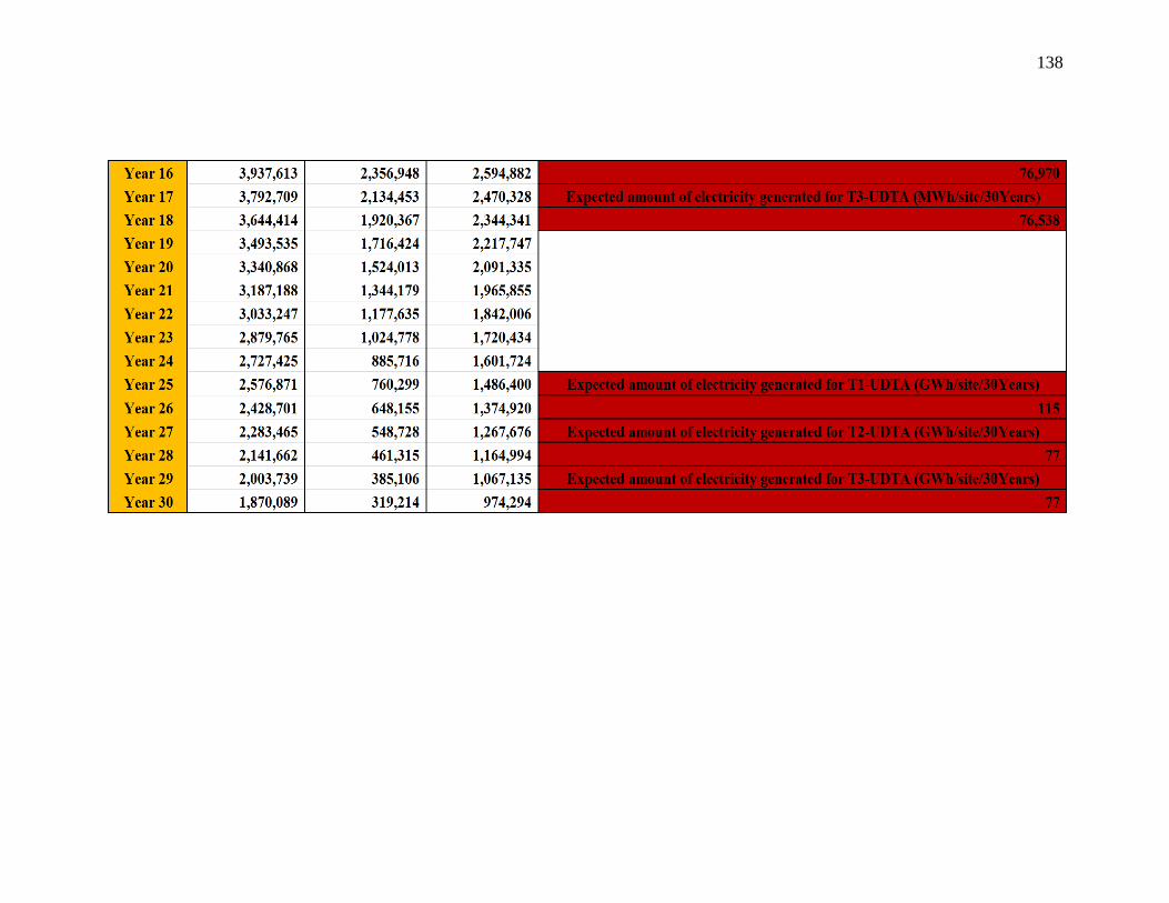
138

139
Table 6.2
Total Expected Amount of Electricity Generated (No Transformer – for UGA)
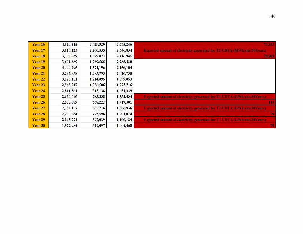
140

141
Table 6.3
Mono-crystalline NPV and Breakeven with Electricity Price of $0.07/kWh (Yes Transformer – to sell)

142

143
Table 6.4
Poly-crystalline NPV and Breakeven with Electricity Price of $0.07/kWh (Yes Transformer – to sell)

144

145
Table 6.5
Thin-film NPV and Breakeven with Electricity Price of $0.07/kWh (Yes Transformer – to sell)

146

147
Table 6.6
Breakeven (year), PV of Benefits, and NPV ($) for T1, T2 and T3 (Yes Transformer – to sell)

148

149
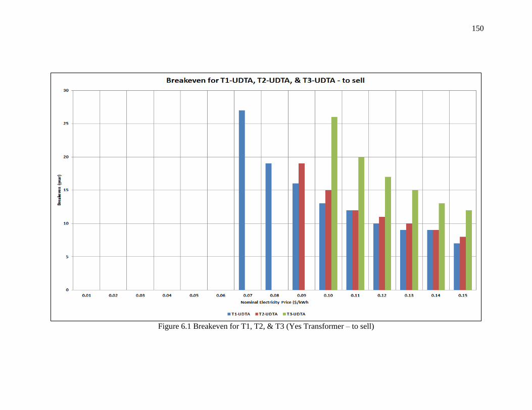
150
Figure 6.1 Breakeven for T1, T2, & T3 (Yes Transformer – to sell)

151
Figure 6.2 Net Present Values for T1, T2, & T3 (Yes Transformer – to sell)

152
Table 6.7
Mono-crystalline NPV and Breakeven at $0.1006/kWh (No Transformer – for UGA)

153

154
Table 6.8
Poly-crystalline NPV and Breakeven at $0.1006/kWh (No Transformer – for UGA)

155

156
Table 6.9
Thin-film NPV and Breakeven at $0.1006/kWh (No Transformer – for UGA)

157

158
Table 6.10
Electricity Price, Breakeven, PV of Benefits, and NPV for T1, T2 and T3 at $0.1066 (No Transformer – for UGA)

159

160

161
Figure 6.3 Breakeven for T1, T2, & T3 at $0.1006/kWh (No Transformer – for UGA)

162
Figure 6.4 Net Present Values for T1, T2, & T3 at $0.1066/kWh (No Transformer – for UGA)

163
CHAPTER 7
(CONCLUSION)
The main objective in this paper is to evaluate the net present value of
installing a photovoltaic (PV) system at the University of Georgia and to
estimate the contribution such a system would make toward meeting UGA’s
CO2 emissions reduction target. While there are many different types of
renewable energy available, this paper analyzes three distinct PV panels (mono-
crystalline, poly-crystalline and thin-film) across three different solar tracking
devices (fixed, single axis tracking, and double axis tracking). Both state and
federal renewable energy programs are included in the analysis. Specific
objectives of the study are to:
Determine the degree to which a 10-acre, ground-installed PV system
in Athens, GA, will help meet all the energy related criteria listed in
the UGA 2020 Strategic plan.
The UGA 2020 strategic plan is to reduce emissions by 20
percent from renewables or fossil fuels relative to baseline of 2010
(Goal 1). And as discussed in section 5.7, scenario A (yes transformer
– to sell) only reached 1.77% and scenario B (no transformer – for
UGA) reached only 1.82%. Therefore, it shows that the first goal can’t
meet the criteria of 20%. Thinking on the positive side, however, if we
were to satisfy the goal for all 20%, we would require 11 more lands
(10 acres) that consist of PV generating system.
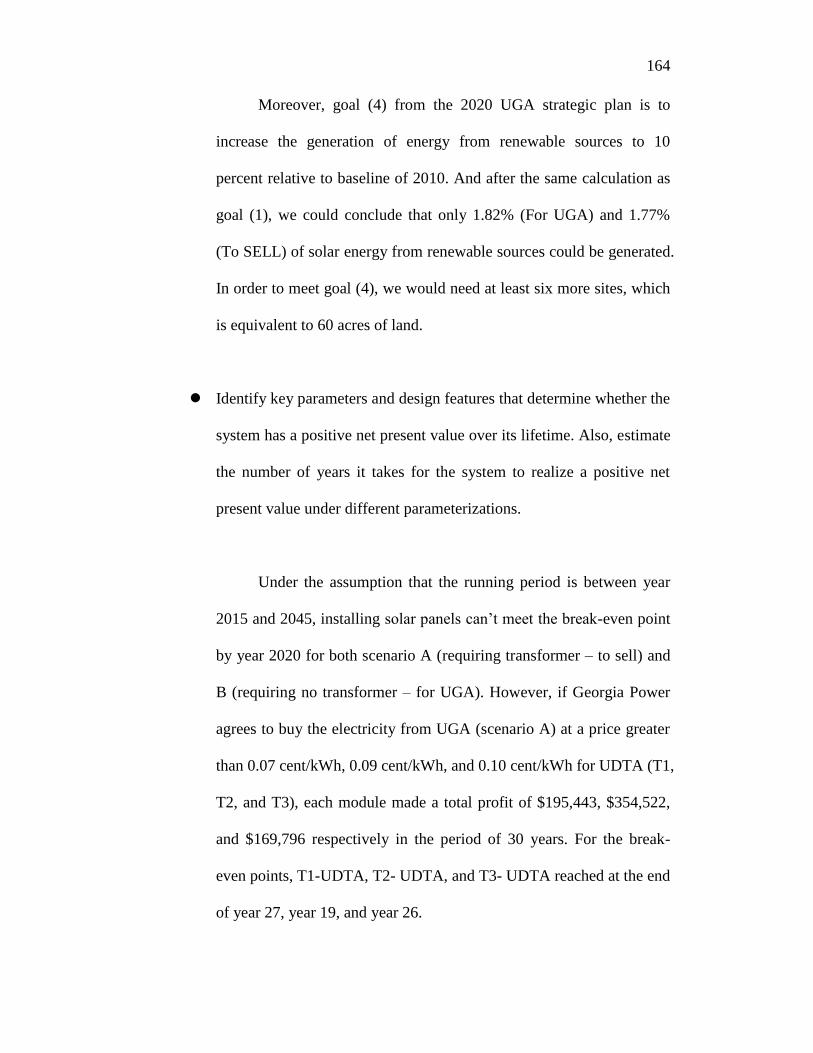
164
Moreover, goal (4) from the 2020 UGA strategic plan is to
increase the generation of energy from renewable sources to 10
percent relative to baseline of 2010. And after the same calculation as
goal (1), we could conclude that only 1.82% (For UGA) and 1.77%
(To SELL) of solar energy from renewable sources could be generated.
In order to meet goal (4), we would need at least six more sites, which
is equivalent to 60 acres of land.
Identify key parameters and design features that determine whether the
system has a positive net present value over its lifetime. Also, estimate
the number of years it takes for the system to realize a positive net
present value under different parameterizations.
Under the assumption that the running period is between year
2015 and 2045, installing solar panels can’t meet the break-even point
by year 2020 for both scenario A (requiring transformer – to sell) and
B (requiring no transformer – for UGA). However, if Georgia Power
agrees to buy the electricity from UGA (scenario A) at a price greater
than 0.07 cent/kWh, 0.09 cent/kWh, and 0.10 cent/kWh for UDTA (T1,
T2, and T3), each module made a total profit of $195,443, $354,522,
and $169,796 respectively in the period of 30 years. For the break-
even points, T1-UDTA, T2- UDTA, and T3- UDTA reached at the end
of year 27, year 19, and year 26.

165
On the other hand, for scenario B (requiring no transformer –
for UGA), we used $0.1066/kWh (10.66Cents/kWh) as fixed end-use
average retail electricity price. And when the nominal price growth
rate was set at 0.10% (1.001), all the module types (UDTA) made a
net profit of $3,291,257, $1,516,856, and $739,330 in the period of 30
years. The breakeven years for the three modules were year 12, year
12 and year 20 respectively.
Determine whether it will be more cost-effective for UGA to use their
own created electricity or create positive financial returns on PV
investment by selling it back to Georgia Power.
When we compared scenario A and B, it would be more cost-
effective for UGA to use their own created electricity rather than
selling it back to Georgia Power (GP) because scenario B (requiring
no transformer – for UGA) made further more profit. Even though GP
decides to increase their current fixed average electricity buyback
price set higher than 0.04cents/kWh, it is most likely impractical for
them because GP is likely to lose money.
166
REFERENCES
Aggarwal SK, Saini LM, Kumar A (2009) Load/price forecasting and managing
demand response for smart grids. Electr Power Energy Syst 31:13–22
Alibaba. “Tilt Single-Axis Tracking (EPR-TSA-6kw). Alibaba. 2013. Web. 23
Mar. 2015. < http://www.alibaba.com/product-detail/GPS-Solar-tracking-
system-Tilt-single_60206749484.html >
"Aluminum 250-ft 10/3 MC Cable." Lowes, n.d. Web. 25 Jan. 2015.
<http://www.lowes.com/pd_220492-295-
68584201_4294722493__?productId=3637696&Ns=p_product_price|1&pl=1&c
urrentURL=%3FNs%3Dp_product_price%7C1%26page%3D1&facetInfo=>.
"American Clean Energy and Security Act of 2009." American Council for an
Energy-Efficient Economy, 2010. Web. 08 Nov. 2014.
<http://www.aceee.org/topics/aces>.
"Amp 12/24/48V Solar PWM Charge Controller W/ Volt & Amp Meter."155
Amp 12/24/48V Solar PWM Charge Controller W/ Volt & Amp Meter. Missouri
Wind and Solar, n.d. Web. 25 Jan. 2015. <http://store.mwands.com/charge-
controllers/155-amp-12/24/48v-solar-pwm-charge-controller-w/volt-amp-
meter/>.
Ardani, Kristen, Galen Barbose, Robert Margolis, Ryan Wiser, David Feldman,
and Sean Ong. "Benchmarking Non-Hardware Balance of System (Soft) Costs
for U.S. Photovoltaic Systems Using a Data-Driven Analysis from PV Installer
Survey Results." (n.d.): n. pag. National Renewable Energy Laboratory and
Lawrence Berkeley National Laboratory, Nov. 2012. Web. 22 Apr. 2015.
<http://www.nrel.gov/docs/fy13osti/56806.pdf>.
Bajpai, P., Singh, S. (2004). Bidding and gaming in electricity market: an
overview and key issues, In: International conference on power systems,
ICPS2004, Kathmandu, Nepal, p. 571–576.
Barlow, M. (2002). A diffusion model for electricity prices, Math Finance, 12(4),
287–98.
Bastian, J., Zhu, J., Banunarayanan, V., Mukerji, R. (1999). Forecasting energy
prices in a competitive market, IEEE Computer Applicat, Power, vol. 12, pp. 40–
45.
UCSUSA (2013a)."Benefits of Renewable Energy Use." Union of Concerned
Scientists, n.d. Web. 09 Nov. 2014. <http://www.ucsusa.org/clean_energy/our-
energy-choices/renewable-energy/public-benefits-of-

167
renewable.html#.VCBiuPl5PpU>.
UCSUSA (2013b)."Benefits of Renewable Energy Use." Union of Concerned
Scientists, n.d. Web. 09 Nov. 2014. <http://www.ucsusa.org/clean_energy/our-
energy-choices/renewable-energy/public-benefits-of-
renewable.html#.VCBiuPl5PpU>.
BigSunEnergy. "TS-T6024AG (iPV)." BIG SUN Energy Technology Inc., 2015.
Web. 18 Apr. 2015. <http://www.bigsun-energy.com/en/products_ipv.php>.
Bloomberg New Energy Finance (2013). Solar Panel Prices Over Time (1977-
2013). Retrieved from http://financialconservation.blogspot.com/2013/01/the-
swanson-effect-pricing-sunshine.html
"Blue Sea Systems 8084." Savinglots, n.d. Web. 25 Jan. 2015.
<http://www.savinglots.com/lotprod.asp?item=8084>.
Blue Selenium Solar, LLC (2013). How Do Solar Panels For Your Home Work.
Retrieved from http://www.bluesel.com/how-does-solar-work/
Bollerslev, T. (1986). Generalized autoregressive conditional heteroscedasticity,
Journal of Econometrics 31, 307-327.
Bordignon S, Bunn DW, Lisi F, Nan F (2013) Combining day-ahead forecasts
for British electricity prices. Energy Econ 35:88–103
Brian McConnell (2013). Comparison of solar energy to conventional energy
source. Retrieved from http://www.resilience.org/stories/2013-04-25/solar-
energy-this-is-what-a-disruptive-technology-looks-like
Bruninga, Bob. "Grid or Off-Grid?" Automatic Packet Reporting System, 04
Apr. 2011. Web. 25 Jan. 2015. <http://www.aprs.org/off-grid-maybe.html>.
Burkhardt et al. (2012) and Whitaker et al. (2012) Photos from iStock/19291390
and iStock/1627655, Top (left to right): Photo from iStock/13737597,
NREL/PIX 18553, iStock/12123595, NREL/PIX 16933, NREL/PIX 18968,
NREL/PIX 19163 Web. 06 Jan. 2015. <
http://www.nrel.gov/docs/fy13osti/56487.pdf>
Business Insights, The Solar Cell Production Global Market Outlook, June 2011,
p. 16-17.
CalculatorSoup Online Calculator Resource. "Triangle Theorems Calculator."
Accessed April 27, 2015.
<http://www.calculatorsoup.com/calculators/geometry-plane/triangle-
theorems.php>

168
California Solar Statistics (2012). Data from the California Solar Initiative
Database. www.californiasolarstatistics.ca.gov/current_data_files/. Accessed
April 22, 2015.
Carr, Geoffrey. "Sunny Uplands." The Economist. The Economist Newspaper,
21 Nov. 2012. Web. 26 Mar. 2015.
<http://www.economist.com/news/21566414-alternative-energy-will-no-longer-
be-alternative-sunny-uplands>.
Catalão, J. P. S., Pousinho, H. M. I., Mendes, V. M. F. (2009). “An artificial
neural network approach for short-term wind power forecasting in Portugal,”
15th International Conference on Intelligent System Applications to Power
Systems, ISAP '09, pp.1-5.
CCSP (2008). Analyses of the effects of global change on human health and
welfare and human systems. A Report by the U.S. Climate Change Science
Program and the Subcommittee on Global Change Research. Gamble, J.L. (ed.),
K.L. Ebi, F.G. Sussman, T.J. Wilbanks, (Authors). U.S. Environmental
Protection Agency, Washington, DC, USA.
i.
Chang FJ, Chiang YM, Chang LC (2007) Multi-step-ahead neural networks for
flood forecasting. Hydrol Sci J Sci Hydrol 52(1)
"CLEAN ENERGY TAX CREDIT (PERSONAL)." U.S Department of Energy,
n.d. Web. 12 Feb. 2015. <http://energy.gov/savings/clean-energy-tax-credit-
personal>
Clean Power Research (2011). How Much Does Solar Cost?. Retrieved from
http://costofsolar.com/management/uploads/2013/06/How-Much-Does-Solar-
Power-Cost.png
CLIMATE CHANGE AND FOOD SECURITY: A FRAMEWORK DOCUMENT.
Rep. ROME,: FOOD AND AGRICULTURE ORGANIZATION OF THE
UNITED NATIONS, 2008. Web. 7 Nov. 2014.
<http://www.fao.org/forestry/15538-
079b31d45081fe9c3dbc6ff34de4807e4.pdf>.
Cohen, Boyd. "Fossil Fuel Emissions Levels." TriplePundit, 28 Apr. 2011. Web.
25 Jan. 2015. <http://www.triplepundit.com/2011/04/shale-gas-fracking-could-
be-part-clean-energy-future/>.
"Consumption for Electricity Generation (Btu) for Electric Utility, Quarterly."
U.S. Energy Information Administration (EIA), 2015. Web. 10 Apr. 2015.
<http://www.eia.gov/electricity/data/browser/#/topic/>.
"Cost of Home Solar Power Systems." Sunrun, 2015. Web. 11 Feb. 2015.

169
<http://www.sunrun.com/solar-lease/cost-of-solar/?
"Cost of Solar Panels - 10 Charts Tell You Everything - Cost of Solar." 10 Cost
of Solar Panels & Cost of Solar Power Charts. Cost of Solar, 1 Dec. 2013. Web.
07 Nov. 2014. <http://costofsolar.com/cost-of-solar-panels-10-charts-tell-you-
everything/>.
"Crystalline Silicon and Thin Film Photovoltaic Results – Life Cycle Assessment
Harmonization." National Renewable Energy Laboratory, 13 Oct. 2013. Web. 06
Jan. 2015. <http://www.nrel.gov/analysis/sustain_lca_pv.html>.
Damodaran, Aswath. "Present Value." Journal of Interlibrary Loan, Document
Delivery & Information Supply 6.3 (1996): 75-76. New York University. Web. 19
Mar. 2015. < http://people.stern.nyu.edu/adamodar/pdfiles/cf2E/tools.pdf>
Daniel Yergin. "Shale Gas as a Game Changer." EnergyBiz, April. 2012. Web. 06
Nov. 2014. < http://www.energybiz.com/magazine/article/257999/shale-gas-
game-changer >.
Database of State Incentives for Renewables & Efficiency (DSIRE a1). “Georgia
Incentives/Policies for Renewables & Efficiency, Clean Energy Tax Credit
(Corporate).” Last review on August 26, 2014. Accessed on November 1, 2014.
(B)
http://www.dsireusa.org/incentives/incentive.cfm?Incentive_Code=GA37F&re=
1&ee=1
Database of State Incentives for Renewable & Efficiency (DSIRE a2).
“Modified Accelerated Cost-Recovery System (MARCS) + Bonus Depreciation
(2008-2012).” Last review on August 26, 2014. Accessed on November 1, 2014.
(B)
http://www.dsireusa.org/solar/incentives/incentive.cfm?Incentive_Code=US06F
&re=1&ee=1
Database of State Incentives for Renewable & Efficiency (DSIRE b). “USDA –
Rural Energy for America Program (REAP) Grants.” Last review on August 26,
2014. Accessed on November 1, 2014. (b)
http://www.dsireusa.org/solar/incentives/incentive.cfm?Incentive_Code=US05F
&re=1&ee=1
Database of State Incentives for Renewables & Efficiency (DSIRE c). “Business
Energy Investment Tax Credit (ITC).” Accessed November 1, 2014. (c)
http://www.dsireusa.org/incentives/incentive.cfm?Incentive_Code=US02F&Stat
e=federal%25C2%25A4tpageid=1&ee=1&re=1
Database of State Incentives for Renewable & Efficiency (DSIRE d). “Georgia
Incentives/Policies for Solar”. Last review on August 26, 2014. Accessed on
170
November 1, 2014. (d)
<http://www.dsireusa.org/solar/incentives/index.cfm?re=1&ee=1&spv=1&st=1
&srp=0&state=GA>
Database of State Incentives for Renewable & Efficiency (DSIRE e).
“FEDERAL Incentives/Policies for Renewable & Efficiency”. Last review on
August 26, 2014. Accessed on November 1, 2014. (e)
<http://www.dsireusa.org/incentives/incentive.cfm?Incentive_Code=US13F&re
=1&ee=1>
Database of State Incentives for Renewable & Efficiency (DSIRE f).
“GEORGIA POWER – SOLAR BUYBACK PROGRAM.” Last review on
August 26, 2014. Accessed on November 1, 2014. (f)
http://www.dsireusa.org/solar/incentives/incentive.cfm?Incentive_Code=GA46F
&re=1&ee=1
Department of Energy 1a. "BUSINESS ENERGY INVESTMENT TAX
CREDIT (ITC)." Accessed April 28, 2015. http://energy.gov/savings/business-
energy-investment-tax-credit-itc.
Department of Energy 1b. "CLEAN ENERGY TAX CREDIT (PERSONAL)."
Accessed April 28, 2015. http://energy.gov/savings/clean-energy-tax-credit-
personal.
"Disadvantages Of Solar Energy." Conserve-Energy-Future, 20 Jan. 2013. Web.
05 Jan. 2015. <http://www.conserve-energy-
future.com/Disadvantages_SolarEnergy.php>.
"Distributed Generation Energy Technology Operations and Maintenance
Costs." NREL, Sept. 2013. Web. 10 Feb. 2015.
http://www.nrel.gov/analysis/tech_cost_om_dg.html
DPW Solar. “Standard Roof/Ground Mounts for 3 Type I.” DPW Solar Inc.
2015. Web. 23 Mar. 2015. <
http://www.dpwsolar.com/index.php/applications/residential/8-residential/23-
ground-mounts-standard-two-tier-and-low-profile>
Easy Solar Poland. "SOLAR SALES TIPS: TRACKING THE SUN -
Easysolar." Easy Solar Poland, 13Aug. 2014. Web. 18 Apr. 2015.
<http://easysolar.co/solar-sales-tips-tracking-the-sun/>.
Ecodirect (2014). BenQ AUO Solar PM250M01-260W - 260 Watt 30 Volt Solar
Panel. SolarDirect, 2014. Web. 25 Jan. 2015. <http://www.ecodirect.com/BenQ-
AUO-Solar-PM250M01-260W-260W-30V-PV-Panel-p/benq-auo-pm250m01-
260.htm>.

171
Electric Power Research Institute. “Addressing Solar Photovoltaic Operations
and Maintenance Challenges.” EPRI Inc., 2010. Web. 18 Apr. 2015.
<http://assets.fiercemarkets.net/public/smartgridnews/1021496AddressingPVOa
MChallenges7-2010_1_.pdf?
Electric Power Research Institute, “Engineering and Economic Evaluation of
Central-Station Solar Photovoltaic Power Plants, Electric Power Research
Institute. 2010. Web. 08 Nov. 2014. http://nextphasesolar.com/wp-
content/uploads/2011/12/NREL-epri-OM-best-practices.pdf
"Electricity Price." U.S. Energy Information Administration (EIA), 2015. Web.
25 Feb. 2015. http://www.eia.gov/electricity/data.cfm#sales
EmperySolar. “Tilt Single-Axis Tracking (EPR-TSA-6kw). Alibaba. 2013. Web.
23 Mar. 2015. < http://www.alibaba.com/product-detail/GPS-Solar-tracking-
system-Tilt-single_60206749484.html >
Enders W (2004) Applied econometric time series. Wiley, New York
"Energy Explorer." Origin News RSS. Origin Energy, 2014. Web. Accessed on
06 Nov. 2014. <http://www.originenergy.com.au/4225/Fossil-fuels>.
"Energy Future Coalition (EFC)." The Opportunity: Economic Growth.
Accessed May 25, 2015. http://energyfuturecoalition.org/Why-We-Must-Act/-
Opportunity-Economic-Growth.
Energy Information Administration. "Most States Have Renewable Portfolio
Standards." Energy Information Administration, 3 Feb. 2012. Web. 08 Nov.
2014. <http://www.eia.gov/todayinenergy/detail.cfm?id=4850>.
ENERGY SOLUTIONS FORUM, "2013 US Solar Industry Jobs Increased by
19.9 Percent." The Solar Foundation. 3 Feb. 2014. Web. 29 Dec. 2014.
<http://breakingenergy.com/2014/02/03/2013-us-solar-industry-jobs-increased-
by-19-9-percent/>.
"Energy Sources." About Energy. Georgia Power, n.d. Web. 09 Nov. 2014.
<http://www.georgiapower.com/about-energy/energy-sources/home.cshtml>.
(University of Georgia, 2012)
EnergyTrend. "TS-T6024AG (iPV)." Alibaba Group. 13 June. 2014. Web. 23
Mar. 2015. <h http://pv.energytrend.com/interview/20140613-6891.html >
Erdogdu, E. (2007). Electricity demand analysis using cointegration and ARIMA
modeling: a case study of Turkey, Energy Policy, 35(2), 1129–46.
"Estimated U.S. Energy Use in 2008." Lawrence Livermore National

172
Laboratory, 2009. Web. 25 Jan. 2015.
<http://www.pennenergy.com/articles/pennenergy/2014/04/llnl-wind-power-
sees-highest-energy-gains-in-u-s-2011-2013.html>.
"Estimated U.S. Energy Use in 2013." Lawrence Livermore National
Laboratory, 2014. Web. 25 Jan. 2015.
<http://www.pennenergy.com/articles/pennenergy/2014/04/llnl-wind-power-
sees-highest-energy-gains-in-u-s-2011-2013.html>.
Eydeland A, Wolyniec K (2003) Energy and power risk management. 2nd edn.
Wiley, Hoboken.
Fainman, D., Raviv, D., and Rosenstreich, R. “Using solar energy to arrest the
increasing rate of fossil-fuel consumption The southwestern states of the USA as
case studies.” Energy Policy 25 (2007): 567-576.
"Federal, State and Local Solar Tax Credits and Rebates." Solar Energy Tax
Credits Rebates. SolarCity, 2012. Web. 08 Nov. 2014.
<http://www.solarcity.com/residential/solar-energy-tax-credits-rebates>.
"Financial Incentives for Solar PV." DSIRE Solar. Database of State Incentives
for Renewable Energy Solar, May 2009. Web. 08 Nov. 2014.
<http://www.solarpowerrocks.com/affordable-solar/solar-incentive-map/>.
FirstSolar (2014). FS Series 3™ Black PV Module. FirstSolar, Jan. 2014. Web.
25 Jan. 2015.
(http://www.firstsolar.com/~/media/documents/data-
sheets/products/module%20data%20sheet/pd-5-401-03_series3black-4_na.ashx>
"Fixed-Tilt vs. Single-Axis Tracker System O&M Comparison." Array
Technologies Inc RSS, 25 July 2014. Web. 18 Apr. 2015.
<http://arraytechinc.com/news-item/fixed-tilt-vs-single-axis-tracker-system-om-
comparison/>.
Fu, Y., Li, Z. (2006). Different models and properties on LMP calculations, In
Proc. IEEE Power Eng. Soc. General Meeting, Montreal, QC, Canada.
Garcia, R.C., Contreras, J., van Akkeren, M., and Garcia, J.B.C. (2005). A
GARCH forecasting model to predict day-ahead electricity prices, IEEE Trans.
Power Syst., 2005, 20, (2), pp. 867–874
Georgia Chamber of Commerce. “Energy Policy Implications of Federal Climate
Change Proposals.” Accessed November 1, 2014.<
http://www.gachamber.com/Environment-Energy/georgiaenergy-policy/>
Georgia Environmental Finance Authority (GEFA). “Clean Energy Property Tax
173
Credit.” <https://gefa.georgia.gov/clean-energy-property-tax-credit>
"GEORGIA GREEN LOANS SAVE AND SUSTAIN PROGRAM." U.S
Department of Energy, n.d. Web. 12 Feb. 2015. <
http://energy.gov/savings/georgia-green-loans-save-and-sustain-program>
Georgia Power (2014). "Energy Sources." Energy Sources. Accessed May 25,
2015. http://www.georgiapower.com/about-energy/energy-sources/home.cshtml.
Georgia Power Company. “Solar Buy Back.” Accessed November 1, 2014. <
http://onlineathens.com/local-news/2014-11-08/construction-well-underway-
mammoth-vogtle-nuclear-site-rural-eastern-georgia>
Goodrich, A. (2012). Personal Communication, May 2012. Golden, CO:
National Renewable Energy Laboratory.
"Greenhouse Effect & Global Warming." Ministry of Environment and Forest,
Government of India, n.d. Web. 25 Jan. 2015.
<http://envis.tropmet.res.in/kidscorner/greenhouse.htm>.
Guan, X., Pepyne, D., Ho, Y.-C. (2001). Gaming and price spikes in electric
power markets, IEEE Trans. Power Syst., vol.16, pp. 402–408.
Guoqiang Sun, Yue Chen, Zhinong Wei, Xiaolu Li, and Kwok W. “Cheung. Day-
Ahead Wind Speed Forecasting Using Relevance Vector Machine.” Published on
May 22, 2014. Accessed on November 1, 2014. <
http://www.hindawi.com/journals/jam/2014/437592/>
Hagan, M. T., Behr, S. M. (1987). The time series approach to short term load
forecasting, IEEE Trans. Power Systems, vol. PWRS-2, no. 3, pp. 785–791.
Hanwhasolar (2014). HSL 60 | Poly UL. Hanwha-solarone, 01 Nov. 2012. Web.
25 Jan. 2015. <http://www.hanwha-
solarone.com/images/stories/documents/products/modules/polycrystalline/en/HS
L60_Poly.pdf>.
Hartman, Dennis. "Tax Credit Vs. Rebate." Ehow, 02 Feb. 2011. Web. 08 Nov.
2014. <http://www.ehow.com/info_7884940_tax-credit-vs-rebate.html>.
Holland, Rob. Break-even Analysis. N.p.: n.p., n.d. Agricultural Extension
Service, the University of Tennessee, Sept. 1998. Web. 19 Mar. 2015.
<https://ag.tennessee.edu/cpa/Information%20Sheets/adc3.pdf>.
Homepower (2007). Ask the Experts: PV Longevity & Degradation.
http://homepower.com. Accessed January 2010.

174
"How Much Electricity Does an American Home Use?" Energy Information
Administration, 20 Feb. 2015. Web. 29 Mar. 2015.
<http://www.eia.gov/tools/faqs/faq.cfm?id=97&t=3>.
"How Much Electricity Is Lost in Transmission and Distribution in the United
States?" U.S. Energy Information Administration (EIA), 07 May 2014. Web. 18
Mar. 2015. <http://www.eia.gov/tools/faqs/faq.cfm?id=105&t=3>
Intergovernmental Panel on Climate Change (2007): Impacts, Adaptation and
Vulnerability, Contribution of Working Group II to the Fourth Assessment
Report of the Intergovernmental Panel on Climate Change (Cambridge Univ
Press, Cambridge, UK) in press.
Intergovernmental Panel on Climate Change (2007). "Climate Change 2007:
Synthesis Report." The 2007 IPCC Report on Climate Change. Accessed May
25, 2015. <https://www.ipcc.ch/publications_and_data/ar4/syr/en/mains1.html>
"IPV Solar Tracker." BIG SUN Energy Technology Inc., 2015. Web. 18 Apr.
2015. <http://www.bigsun-energy.com/en/products_ipv.php>.
Jablonska, M. (2008). Analysis of outliers in electricity spot prices with example
of New England and New Zealand markets, Master's thesis, Lappeenranta
University of Technology.
Jacques, Carole. "Solar to Become Competitive with Natural Gas by
2025."NEWS & EVENTS. Lux Research, Inc., 3 Dec. 2013. Web. 08 Nov. 2014.
<http://www.luxresearchinc.com/news-and-events/press-releases/read/solar-
become-competitive-natural-gas-2025>.
Jordan, Dirk, and Sarah Kurtz. "Photovoltaic Degradation Rates — An
Analytical Review." June 1, 2012. Accessed April 24, 2015.
<http://www.nrel.gov/docs/fy12osti/51664.pdf>
Kaminski V (2013) Energy markets. Risk Books, New York.
Kerr, Andy. "To Track or Not to Track?" N.p., May 2013. Web. 23 Mar. 2015.
<http://www.homepower.com/articles/solar-electricity/design-installation/track-
or-not-track>.
Kirsche, Kevin. UGA Energy Usage from 2006-2014 (Athens, Georgia). 2014.
Raw data. University of Georgia, Athens, GA.
Landau, Charles. “Optimum Tilt of Solar Panels.” April 16, 2014. Accessed
April 27, 2015. <htttp://www.solarpaneltilt.com/>
Langen, C. (2010). “Complexity Cost and Economies of Scale: Why Residential

175
Customers in Germany Pay 25% Less for a PV System that U.S. Customers.”
Proceedings of Solar Power International. Washington, DC: Solar Energy
Industries Association.
"Life Cycle Assessment (LCA)." Environmental Protection Agency, 2014. Web.
06 Jan. 2015. <http://www.epa.gov/nrmrl/std/lca/lca.html#define>.
"LIFE CYCLE ANALYSIS (LCA) OF ENERGY TECHNOLOGY AND
PATHWAYS." The National Energy Technology Laboratory (NETL), 2014.
Web. 10 Jan. 2015. <http://www.netl.doe.gov/research/energy-analysis/life-
cycle-analysis>.
“Life Cycle Greenhouse Gas Emissions from Solar Photovoltaics.” Nov. 2012.
Web. 06 Jan. 2015. < http://www.nrel.gov/docs/fy13osti/56487.pdf>
Machol, Rizk. 2013. Economic value of U.S. fossil fuel electricity health
impacts. Environment International 52 75–80.
Maehlum, Mathias Aarre. "Are Solar Panel Tracking Systems Really
Necessary?" Energy Informative Organization, 14 Aug. 2013. Web. 25 Jan.
2015. <http://energyinformative.org/solar-panel-tracking-systems>.
"Map of Athens, Georgia." University of Georgia, 2014. Web. 25 Jan. 2015.
<http://eagle.camplan.uga.edu/OUAGISWEB/CampusMap/>.
Mathes, Lara D. Map of Capacity Potential for Installing Solar Panel at UGA
Areas. 2014. Raw data. University of Georgia, Athens, GA.
McConnell, Brian. "Solar Energy : This Is What A Disruptive Technology Looks
Like." RSS. Resilience.org, 25 Apr. 2013. Web. 07 Nov. 2014.
<http://www.resilience.org/stories/2013-04-25/solar-energy-this-is-what-a-
disruptive-technology-looks-like>.
Meck, Reme. "Calculating Tilted Array Spacing." Accessed April 24, 2015.
http://www.affordable-solar.com/Learning-Center/Building-a-
System/Calculating-Tilted-Array-Spacing.
Michael. "Types of Solar Energy and Solar Power." Types of Solar Energy and
Solar Power. N.p., 2008. Web. 08 Nov. 2014. <http://www.solar-energy-at-
home.com/types-of-solar-energy.html>.
"MidNite Solar 16 Circuit Combiner." Solar Panel Store, n.d. Web. 25 Jan. 2015.
<http://www.solarpanelstore.com/solar-power.elec-parts.readywatt-combiner-
boxes.midnite_mnpv16.info.1.html>.
Moghram, I., Rahman, S. (1989). Analysis and evaluation of five short-term load
176
forecasting techniques, IEEE Trans. Power Systems, vol. 4, no. 4, pp. 1484–
1491.
"More Solar Coming to Georgia: Are You Ready? - Solar Outreach Partnership."
Solar Outreach Partnership, 30 July 2013. Web. 10 Feb. 2015. <
http://solaroutreach.org/2013/07/30/700mw_georgia/#.VNq6KPmG9kY>
"Most States Have Renewable Portfolio Standards." Energy Information
Administration, 3 Feb. 2012. Web. 08 Nov. 2014.
<http://www.eia.gov/todayinenergy/detail.cfm?id=4850>.
M.L. Weitzman. “Why the far-distant future should be discounted at its lowest
possible rate?” Journal of Environmental Economics and Management, 36
(1998), pp. 201–208
Nadel, Steven. Energy Efficiency Tax Incentives in the Context of Tax Reform.
Washington, DC: American Council for an Energy-Efficient Economy,
2012. Energy Efficiency Tax Incentives in the Context of Tax Reform. American
Council for an Energy-Efficient Economy, July 2012. Web. 08 Dec. 2014.
<http://aceee.org/files/pdf/white-paper/energy-efficiency-tax-incentives.pdf>.
"National Solar Jobs Census 2013." The Solar Foundation. N.p., 2013. Web. 10
Jan. 2015. <http://thesolarfoundation.org/>.
National Weather Service. "Athens, Georgia Weather." City State & Zipcode
Search Page. April 27, 2015. Accessed April 27, 2015.
http://forecast.weather.gov/MapClick.php?CityName=Athens&state=GA&site=
FFC&lat=33.9553&lon=-83.3937#.VT6WpyF_NBc
"Net Metering & Photovoltaic Meters." PacificPower, 2014. Web. 25 Jan. 2015.
<https://www.pacificpower.net/env/nmcg/nm/oregon/nmapm.html>.
Nima Amjady and Farshid Keynia. “Day ahead price forecasting of electricity
markets by a mixed data model and hybrid forecast method.” Published on June
11, 2008. Accessed on November 1, 2014. Electrical Power and Energy Systems
30 (2008) 533–546
"No 'Plan B' for Climate Action as There Is No 'Planet B, Says UN Chief."News.
United Nations, 21 Sept. 2014. Web. 9 Nov. 2014.
<http%3A%2F%2Fwww.un.org%2Fapps%2Fnews%2Fstory.asp%3FNewsID%3
D48766%23.VF8VHfmG_cc>.
Northern Arizona Wind & Sun. “Standard Roof/Ground Mounts for 3 Type I.”
Northern Arizona Wind & Sun. 2015. Web. 23 Mar. 2015. <http://www.solar-
electric.com/solar-panels-mounts-kits-accessories/panel-mounts/mounts-

177
dp/romo/stromo/dpwmoduletypei.html.
Nowotarski J, Raviv E, Trück S, Weron R (2014) An empirical comparison of
alternative schemes for combining electricity spot price forecasts. Energy Econ.
doi:10.1016/j.eneco.2014.07.014
"NREL Sets New World Record with Two-Junction Solar Cell - Energy
Informative." Energy Informative Org, 29 Aug. 2013. Web. 08 Dec. 2014.
<http://energyinformative.org/nrel-efficiency-record-two-junction-solar-cell>.
NREL PVWatts. "PVWatts® Calculator." National Renewable Energy
Laboratory, 2014. Web. 25 Jan. 2015.
<http://rredc.nrel.gov/solar/calculators/pvwatts/version1/change.html>.
NREL PVWatts1. "PVWatts® Calculator." National Renewable Energy
Laboratory, 2014. Web. 25 Jan. 2015. <http://pvwatts.nrel.gov/index.php>.
NREL PVWatts2."PVWatts® Calculator." National Renewable Energy
Laboratory, 2014. Web. 25 Jan. 2015.
<http://rredc.nrel.gov/solar/calculators/pvwatts/version1/>.
O'Connor, Mary I., Andrea Anton, John F. Bruno, Michael F. Piehler, and Dina
M. Leech. "Warming and Resource Availability Shift Food Web Structure and
Metabolism." Public Library of Science Organization, 25 Aug. 2009. Web. 9
Nov. 2014.
<http://www.plosbiology.org/article/info%3Adoi%2F10.1371%2Fjournal.pbio.1
000178>.
"Off-Grid System." Pierro Construction, 2012. Web. 25 Jan. 2015.
<http://www.pierrosolar.com/why/about-solar-panels/on-grid-vs-off-grid>.
On-Grid System." Pierro Construction, 2012. Web. 25 Jan. 2015.
<http://www.pierrosolar.com/why/about-solar-panels/on-grid-vs-off-grid>.
Owens, Gene. "Best Practices Guide: Economic & Financial Evaluation of
Renewable Energy Projects." U.S. Agency for International Development Office
of Energy, Environment & Technology Global Bureau Environment Center, 1
June 2002. Web. 19 Mar. 2015.
"Photovoltaics." Library. ENGINEERING.com, Inc., n.d. Web. 05 Nov. 2014.
<http://www.engineering.com/SustainableEngineering/RenewableEnergyEngine
ering/SolarEnergyEngineering/Photovoltaics/tabid/3890/Default.aspx>.
Pino R, Parreno J, Gomez A, Priore P (2008) Forecasting next-day price of
electricity in the Spanish energy market using artificial neural networks. Eng
Appl Artif Intell 21:53–62

178
Prices and Factors Affecting Prices. Energy Information Administration, 7 Oct.
2014. Web. 07 Nov. 2014.
<http://www.eia.gov/EnergyExplained/index.cfm?page=electricity_factors_affec
ting_prices>.
"Price Quotes". http://pv.energytrend.com/. Archived from the original on 26
June 2014. Retrieved 26 June2014.
Public Utility Regulatory Policies Act of 1978 (PURPA). U.S. Energy
Department, n.d. Web. 08 Dec. 2014. <http://energy.gov/oe/services/electricity-
policy-coordination-and-implementation/other-regulatory-efforts/public>.
Raviv E, Bouwman KE, van Dijk D (2013) Forecasting day-ahead electricity
prices: Utilizing hourly prices. Tinbergen Institute Discussion Paper 13-068/III.
Available at SSRN: http://dx.doi.org/10.2139/ssrn.2266312.
RBI Solar Company. Solar Shading Calculator. 2015. Accessed May 5, 2015.
http://www.rbisolar.com/solar-shading-calc/.
"Renewable Portfolio Standards." Policy Basics: State and Local Governments.
National Renewable Energy Laboratory, 2014. Web. 08 Nov. 2014.
<http://www.nrel.gov/tech_deployment/state_local_governments/basics_portfoli
o_standards.html>.
"RESIDENTIAL RENEWABLE ENERGY TAX CREDIT." U.S Department of
Energy, n.d. Web. 12 Feb. 2015. http://energy.gov/savings/residential-renewable-
energy-tax-credit
Riebeek, Holli and Simmon, Robert. "Global Warming: Feature
Articles." Global Warming : Feature Articles. National Aeronautics and Space
Administration, 6 June 2010. Web. 05 Nov. 2014.
<http://earthobservatory.nasa.gov/Features/GlobalWarming/>.
Riebeek, Holli and Simmon, Robert. "Temperature Histories from Paleoclimate
Data." How Is Today’s Warming Different from the Past? 10 Aug. 2007. Web. 7
Nov. 2014. <http://earthobservatory.nasa.gov/Features/GlobalWarming/>.
Rinaldi, Nicholas. "Solar PV Module Costs to Fall to 36 Cents per Watt by
2017." N.p., 18 June 2013. Web. 26 Mar. 2015.
<http://www.greentechmedia.com/articles/read/solar-pv-module-costs-to-fall-to-
36-cents-per-watt>.
Robinson, T.A. (2000). Electricity pool prices: a case study in nonlinear time-
series modelling, Applied Economics, 32(5), 527-532.
Rodriguez, C.P., Anders, G.J. (2004). Energy price forecasting in the Ontario

179
competitive power system market. IEEE Trans Power Syst;19(3):366–74.
Sachs, Emanuel. "Rising Solar’s Falling Prices." Grid Parity. Massachusetts
Institute of Technology, 2009. Web. 08 Nov. 2014.
<https://www.greenwizard.com/2011/11/rising-solars-falling-prices/>.
Schonek, Jacques. "How Big Are Power Line Losses? - Schneider Electric
Blog." Schneider Electric Blog. March 25, 2013. Accessed April 23, 2015.
<http://blog.schneider-electric.com/energy-management-energy-
efficiency/2013/03/25/how-big-are-power-line-losses/.>
"Short-Term Energy Outlook: Table 7c. U.S. Regional Electricity Prices." U.S.
Energy Information Administration - EIA - Independent Statistics and Analysis,
10 Mar. 2015. Web. 04 Apr. 2015. <http://www.eia.gov/forecasts/steo/data.cfm>.
"Solar-Log Online Energy Monitoring System." Lowes, n.d. Web. 25 Jan. 2015.
< http://www.lowes.com/pd_380838-37956-029-
06020_0__?productId=3580544 >.
"Solar Buy Back." Georgia Power, n.d. Web. 12 Feb. 2015. <
http://www.georgiapower.com/energy-efficiency/green/solar-buyback.cshtml>
Solar Energy Industries Association. “Concentrating Solar Power.” 2014.
Accessed November 1, 2014.< http://www.seia.org/policy/solar-
technology/concentrating-solar-power>
Solar Energy Industries Association (SEIA). “Investment Tax Credit (ITC).”
Accessed November 1, 2014. http://www.seia.org/research-resources/case-solar-
investment-tax-credit-itc
Solar Energy Industries Association. “U.S. Solar Market Insight Report, 2011
Year-in-Review, Executive Summary.” 2014. Accessed November 1, 2014.
<http://www.seia.org/policy/solar-technology/photovoltaic-solar-electric>
"Solar Irradiation in Athens, GA, USA." Synergy Environment Engineers
(India), 2014. Web. 25 Jan. 2015.
<http://www.synergyenviron.com/tools/solar_insolation.asp?loc=athens+ga>.
"Solar Photovoltaic Technology Basics." Learning about Renewable Energy.
National Renewable Energy Laboratory, 2014. Web. 05 Nov. 2014.
<http://www.nrel.gov/learning/re_photovoltaics.html>.
"Solar Power Installation Breakdown - Solar Power." Solarpower.org, 2013.
Web. 10 Feb. 2015.

180
"Solar Radiation at Athens." University of Georgia, Department of Geography,
2014. Web. 25 Jan. 2015. <http://geography.uga.edu/>.
"SOLAR SALES TIPS: TRACKING THE SUN - Easysolar." Easy Solar Poland,
13Aug. 2014. Web. 18 Apr. 2015. <http://easysolar.co/solar-sales-tips-tracking-
the-sun/>.
"Step-up (15kv) Power Transformer - Buy Step-up Transformer,Transformer
Power,15kv Transformer Product on Alibaba.com." Alibaba, n.d. Web. 19 Feb.
2015.
Sunny Central 1,000CP XT. SMA, 2014. Web. 25 Jan. 2015. <
http://files.sma.de/dl/15867/SCCPUS-DUS134831W.pdf>.
<http://www.proinsosolar.com/grid-tie-solar-inverters/sma-sunny-central-
c_32_53.html>.
Sunny Central 500CP XT. SMA, 2014. Web. 25 Jan. 2015. <
http://files.sma.de/dl/15867/SCCPUS-DUS134831W.pdf>.
<http://www.proinsosolar.com/grid-tie-solar-inverters/sma-sunny-central-
c_32_53.html>.
SUNNY Tripower 24,000TL-US. SMA, 2014. Web. 25 Jan. 2015. <
http://files.sma.de/dl/21561/STPTL-US12-24-DUS143110W.PDF >. <
http://www.proinsosolar.com/grid-tie-solar-inverters/sma-sunny-tripower-
c_32_60.html >.
Synergy Environment Engineers "Solar Irradiation in Athens, GA, USA."
Synergy Environment Engineers (India), 2014. Web. 25 Jan. 2015.
<http://www.synergyenviron.com/tools/solar_insolation.asp?loc=athens+ga>.
"Topper Sun's IPV Solar Tracker: Greater Power, Better Reliability and More
Cost Effective." EnergyTrend, 13 June 2014. Web. 18 Apr. 2015.
<http://pv.energytrend.com/interview/20140613-6891.html>.
Tseng, F. M., Yu, H.C., Tzeng, G.H. (2002). Combining neural network model
with seasonal time series ARIMA model, Technological Forecasting and Social
Change, 69, 71–87.
Tverberg, Gail. "What Happens When Oil and Other Fossil Fuels Deplete."What
Happens When Oil and Other Fossil Fuels Deplete. Oil Price, 06 July 2010.
Web. 07 Nov. 2014. <http://oilprice.com/Energy/Energy-General/What-
Happens-When-Oil-And-Other-Fossil-Fuels-Deplete.html>.
University of Georgia Department of Geography. "Solar Radiation at Athens."
University of Georgia, Department of Geography, 2014. Web. 25 Jan. 2015.
<http://geography.uga.edu/>.

181
"University of Georgia 2020 Strategic Plan." The University of Georgia, 30 Oct.
2012. Web. 24 Nov. 2014. <http://sustainability.uga.edu/about/>.
U.S. Department of Energy (2014). History of Solar Energy to Oil & Natural
Gas. Retrieved from http://www.nrel.gov/docs/fy14osti/62558.pdf
U.S. Department of Energy. “Renewable Portfolio Standards.” Advanced
Research Projects Agency- Accessed November 1, 2014.
<http://energy.gov/funding-financing-energy-projects>
U.S. Energy Information Administration. “Major Components of U.S. Average
Electricity Price, 2011.” Last review on September 09, 2014. Accessed on
October 1, 2014.
<http://www.eia.gov/energyexplained/index.cfm?page=electricity_factors_affect
ing_prices>
U.S. Energy Information Administration. “Short-Term Energy Outlook, 2014.” ”
Last review on September 09, 2014. Accessed on October 1, 2014.
<http://www.eia.gov/forecasts/steo/>
"U.S. Greenhouse Gas Emissions by Gas, 1990-2012." Environmental Protection
Agency, 2014. Web. 25 Jan. 2015.
<http://www.epa.gov/climatechange/ghgemissions/usinventoryreport.html>.
Vote Solar (2011). Project Permit Interactive Permitting Map.
http://votesolar.org/cityinitiatives/project-permit/. Accessed April 22, 2015.
"WHAT IS GRID PARITY?" Lear More. Renewable Energy Advisors, n.d. Web.
08 Nov. 2014. <http://www.renewable-energy-advisors.com/learn-more-2/what-
is-grid-parity/>.
“What’s up with the weather: the debate: Stephen H. Schneider”
http://www.pbs.org/wgbh/warming/debate/schneider.html. PBS Nova &
Frontline. Retrieved 2007-04-13.
Weigend, Andreas S., Ashok N. Srivastava, and Morgan Mageas. Nonlinear
Gated Experts For Time Series: Discovering Regimes and Avoiding
Overfitting (1995): n. pag. Web. 7 Nov. 2014.
<http://digitool.library.colostate.edu///exlibris/dtl/d3_1/apache_media/L2V4bGli
cmlzL2R0bC9kM18xL2FwYWNoZV9tZWRpYS8xNjc3MTc=.pdf>.
Weron, R. (2006). Modeling and forecasting electricity loads and prices: A
statistical approach, Volume 396 of Wiley, pp. 125-127.
Wen Yu, Haibo He, Nian Zhang. “Advances in Neural Networks.” Published on
May 26, 2009. Accessed on November 1, 2014. ISBN 978-3-642-01507-6

182
"Why Solar?" Department of Energy Statistics, n.d. Web. 06 Nov. 2014. <
http://www.lennox.com/solar-solutions/why-solar.asp >.
Wood, I. Daniel. "Energy.gov." Fossil. U.S. Energy Department, 2014. Web.
Accessed on 05 Nov. 2014. <http://energy.gov/science-innovation/energy-
sources/fossil>.
World Energy Consumption by fuel (Quadrillion Btu). U.S. Energy Information
Adminstitration, 25, July, 2013. Web. 05 Nov. 2014. <
http://www.eia.gov/todayinenergy/detail.cfm?id=12251>
World Energy Perspective: Cost of Energy Technologies. Rep. London: World
Energy Council, 2013. Web. 8 Nov. 2014. <http://www.worldenergy.org/wp-
content/uploads/2013/09/WEC_J1143_CostofTECHNOLOGIES_021013_WEB
_Final.pdf>.
Wu, L., Shahidehpour, M. (2010). A hybrid model for day-ahead price
forecasting,” IEEE Trans. Power Syst., vol. 25, no. 3, pp. 1519–1530.
Yamin, H. Y., Shahidehpour, S. M., Li, Z. (2004). Adaptive short-term
electricity price forecasting using artificial neural networks in the restructured
power markets. Electrical Power Energy Syst, 26, 571–81.
Zhang, G. P., Qi, M. (2005). Neural network forecasting for seasonal and trend
time series, European Journal of Operational Research, 160, 501–514.
"2010 EGRID Subregion GHG Output Emission Rates (PDF)." Environmental
Protection Agency, 24 Jan. 2014. Web. 03 Apr. 2015.
<http://www.epa.gov/cleanenergy/energy-resources/egrid/index.html>.

183
APPENDIX A
Size for the Different Module, Array, and Site
Maximum # of
Module Length (m)
Available per Array
Actual # of Module
Length Available per
Array
Maximum # of
Module Width (m)
Available per
Array
Actual # of Module
Width Available per
Array
Total # of
Modules
Available per
Array
T1-TFA
T2-TFA
T3-TFA
1.00
1.00
1.38
1
1
1
4.00
4.00
6.67
4
4
6
4
4
6
T1-TSTA
T2-TSTA
T3-TSTA
6.00
6.00
8.28
6
6
8
2.97
2.97
4.95
3
3
5
18
18
40
T1-
UDTA
T2-
UDTA
T3-
UDTA
4.00
4.00
5.50
4
4
5
6.20
6.20
10.33
6
6
10
24
24
50
Maximum # of
Array Length (m)
Available per Site
Actual # of Array
Length Available per
Site
Maximum # of
Array Base (m)
Available per Site
Actual # of Array
Base Available per
Site
Total # of Arrays
Available per Site
T1-TFA
T2-TFA
T3-TFA
110.48
110.48
110.48
110
110
110
17.71
17.71
17.71
17
17
17
1,870
1,870
1,870
T1-TSTA 77.85 77 7.16 7 539
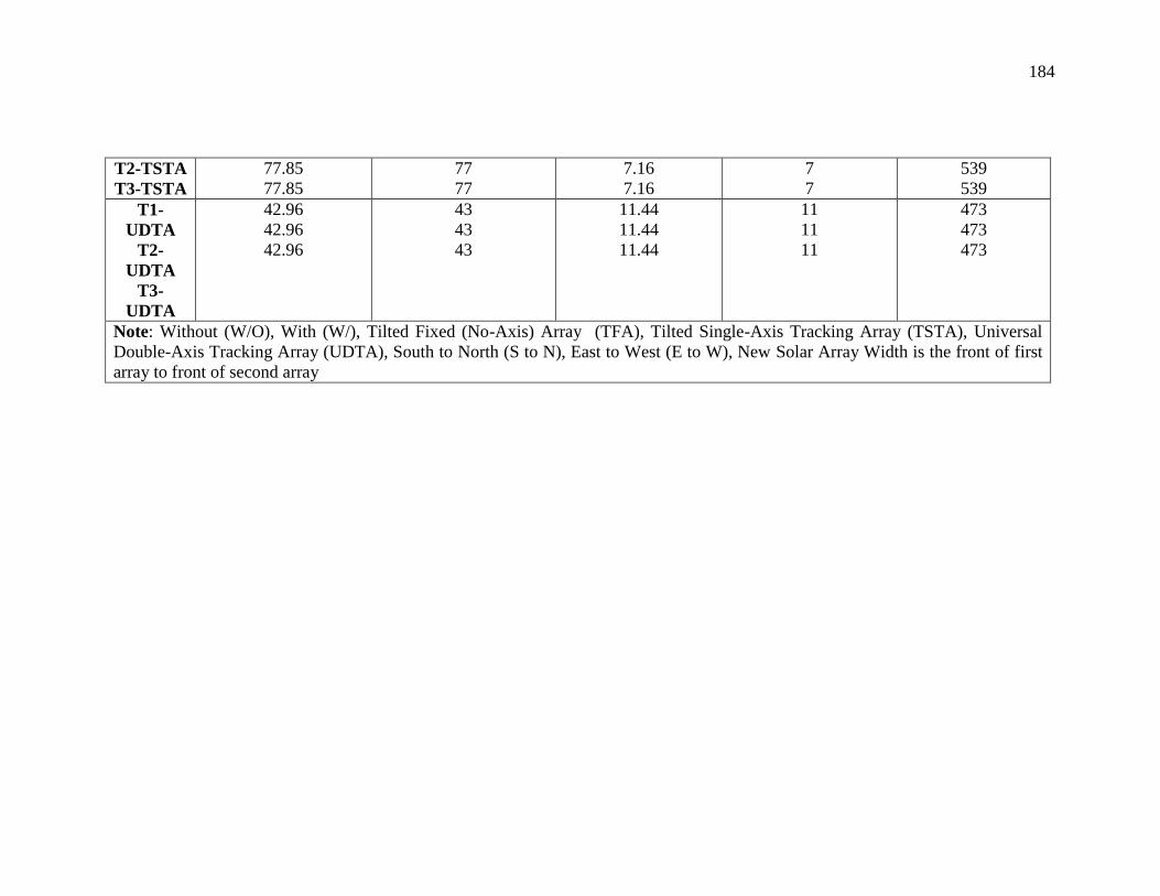
184
T2-TSTA
T3-TSTA
77.85
77.85
77
77
7.16
7.16
7
7
539
539
T1-
UDTA
T2-
UDTA
T3-
UDTA
42.96
42.96
42.96
43
43
43
11.44
11.44
11.44
11
11
11
473
473
473
Note: Without (W/O), With (W/), Tilted Fixed (No-Axis) Array (TFA), Tilted Single-Axis Tracking Array (TSTA), Universal
Double-Axis Tracking Array (UDTA), South to North (S to N), East to West (E to W), New Solar Array Width is the front of first
array to front of second array

185
APPENDIX B
Derate Factors Used
Component of
Derate Factors
Range Definition
PV module
nameplate DC
(a)
0.800 – 1.050
(0.950)
The nameplate rating loss accounts for the accuracy of the manufacturer’s nameplate rating.
Field measurements of the electrical characteristics of photovoltaic modules in the array
may show that they differ from their nameplate rating. A nameplate rating loss of 5%
indicates that testing yielded power measurements at STC that were 5% less than the
manufacturer’s nameplate rating.
Transformer &
Transmission Line
(b)
0.980 – 0.990
(0.985)
Discussed more in the later section 5.3.4.5
Mismatch
(c)
0.970 – 0.995
(0.980)
Electrical losses due to slight differences caused by manufacturing imperfections between
modules in the array that cause the modules to have slightly different current-voltage
characteristics.
Diodes and
connections
(d)
0.990 – 0.997
(1.00)
Resistive losses in electrical connectors in the system.
DC wiring
(e)
0.970 – 0.990
(0.980)
Resistive losses in the DC wires connecting modules, inverters, and other parts of the
system.
AC wiring
(f)
0.980 – 0.993
(0.990)
Resistive losses in the AC wires connecting modules, inverters, and other parts of the
system.
Soiling (dirt, snow)
(g)
0.300 – 0.995
(0.995)
Losses due to dirt, snow, and other foreign matter on the surface of the PV module that
prevent solar radiation from reaching the cells.

186
System availability
(h)
0.000 – 0.995
(0.980)
Reduction in the system’s output caused by both scheduled and unscheduled system shut
down for maintenance, grid outages, and other operational factors.
Shading (Reduction
Factor)
(i)
0.000 – 1.000
(1.000)
Reduction in the incident solar radiation from shadows caused by objects near the array
such as buildings or trees, or by self-shading for fixed arrays or arrays with two-axis
tracking.
Light-Induced
Degradation
(j)
0.980 –
0.990
(0.980)
Effect of the reduction in the array’s power during the first few months of its operation
caused by light-induced degradation of photovoltaic cells.
Age
(k)
0.700 – 1.000
(1.000)
Effect of weathering of the photovoltaic modules on the array’s performance over time.
Overall DC to AC
DF
0.854
0.842
W/O Transformer
= a × b × c × d × e × f × g × h × i × j × k
= 0.854
W Transformer (leaving out b)
= a × b × d × e × f × g × h × i × j × k
= 0.842
Source: NREL PVWATTS, 2014; Jacuqes, 2013

187
APPENDIX C
Technical and Price Specification for the Balance of System (BoS)
Model Input Definition
Transformer Price: $15,000
Model: 15kv Step-up power transformer
Details: Each monitor supports voltage capacity of 40,000kVA (38,000kWh) and lose 3% of the energy from the
DC System.
Monitor Price: $508.98
Details: Each monitor can support the size of 1,000kW inverter.
Meters While PV meter helps to keep track of how much energy is produced by the solar panels, net meter is used to keep
track of energy flowing to and from your utility provider (Pacific Power, 2014).
Price: $429.00
Details: Can hold up to 12,500 Watts (12.5kW)
Combiner
Box
Name: Circuit Combiner Box
Model: MNPV16
Holds Output of: 100,000 W (100kW)
Price: $319.20
Wiring Name: Aluminum MC Cable / Model Number: 68584201
Outside / Inside: Aluminum / Copper
Length: 250ft = 76.2m
Price: $280
AC Main
Breaker
Name: Schneider Electric
Model: Square D QO140M200 Convertible Main Breaker Load Center
Details: requires only 1 for each system
Price: $1,011.46

188
Source for Transformer: Alibaba, 2014
Source for Monitor: Lowes, 2015
Source for Meters: MW&S, 2015
Source for Combiner Box: Solar panel store, 2015
Source for Wiring: Lowes, 2015
Source for AC Main Breaker: Saving lots, 2015