An Economic History of the Failure of Broiler Futures

8/10/2019 An Economic History of the Failure of Broiler Futures

http://slidepdf.com/reader/full/an-economic-history-of-the-failure-of-broiler-futures 1/39

An Economic History of the Failure of Broiler Futures

S. Aaron Hegde

North Carolina State University

Raleigh, NC 27695-8110

[email protected] ∗

Paper prepared for presentation at the American Agricultural Economics Association Annual Meeting, Denver, Colorado,

August 1 - 4, 2004

∗Copyright 2004 by Hegde. All rights reserved. Readers may make verbatim copies of this document for non-commercial purposes by any means, provided that this copyright notice appears on all such copies

1



Abstract

Hedging with a futures market is a risk management alternative available to

producers of most agricultural commodities. However, such an option is unavailable

to broiler growers as there are no active broiler futures. Over the last 40 years

there were three occasions during which futures for broilers were available. Each

of the three markets failed to catch on and was thus removed from trading. We

investigate the reasons for the failures time and time again. Using an econometric

model, we find that the lack of an efficient hedge was a major reason the broiler

futures collapsed.

2



1 Introduction

Knoeber and Thurman (1995) find that 84% of production risk is transferred from broiler

growers to integrators via contract production. This is due to a lack of the market price

of broilers in calculating grower compensation. From the grower perspective this is a

form of risk management. In fact, this is the dominant form of risk management in the

broiler industry today. Typically, producers of agricultural commodities can use futures

markets, in addition to contracting, to mitigate the variance in the market price of their

commodity. Currently, there are futures markets for most agricultural commodities with

large cash markets such as cattle, hogs, corn and wheat to name a few. The exception,

however, is the broiler industry which is probably one of the larger agricultural industries

to not have its own futures market. But this was not always the case.

On July 17, 1993, broiler futures traded for what would be the last time on any futures

exchange. Prior to this, the very first time broiler futures ever traded on any exchange

was in 1968, when they began trading on the Chicago Board of Trade (CBOT). But that

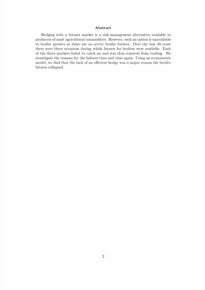
particular futures market stopped trading in December of 1980 (see figure 1 for a timeline

of broiler futures markets). This was neither the first time a commodity futures market

had failed, nor would it be the last. In fact, the Chicago Mercantile Exchange (CME) tried

unsuccessfully to market broiler futures during the 1980s and again during the 1990s 1.

Onion futures are perhaps the most infamous contract to stop trading. It will take an

act of Congress to reinstate the trading of onion futures. In 1958, Congress passed a bill2

1Iced broiler futures were traded on CBOT from 1968-1980 (BrI) while the CME traded broilers from1979-1982 (BrII) and later from 1991-1993 (BrIII).

2USC:Title 7:Section 13-1: (a) No contract for the sale of onions for future delivery shall be made onor subject to the rules of any board of trade in the United States. (b) Any person who shall violate theprovisions of this section shall be deemed guilty of a misdemeanor and upon conviction thereof be fined

3



BrI: 8/68-12/80

BrII: 11/79-8/82

BrIII: 12/90-7/93

BrIII

8/68 7/9312/908/8212/8011/79

BrII

BrI

Figure 1: Broiler Futures Timeline

banning the sale of onion futures3. As of yet, this law has not been repealed.

After a brief seventeen-month existence between 1987 and 1988, high fructose corn

syrup contracts (HCF-55) were also permanently delisted from the Minneapolis Grain

Exchange (Thompson, Garcia and Wildman 1996). There are now defunct futures markets

for potatoes, GNMA Collateral Depository Receipts (a financial futures), boneless beef,

wine, apples and even corn yields. But not every poorly performing futures contract is

necessarily delisted. At times, futures contracts are temporarily removed from exchanges

to be brought back after revision of certain contract specifications. Such was the case

during February of 1997 when live hog futures were discontinued and later replaced by

lean hog futures4. This begs the question: why do some commodities, such as wheat, live

not more than $5,000. This ban was enacted as a result of complaints from growers that futures tradingincreased volatility of cash prices.

3See (Gray 1963), (Johnson 1977) and (Higgens and Holcombe 1980) for details about the collapse of onion futures.

4The contract specifications were changed to reflect cash settlements rather than delivery of hogs.

4



cattle, and gold to name a few, continue to enjoy successful futures markets, while those

for other commodities such as broilers fail? The objective of this article is to provide an

economic history of broiler futures and to explore the reasons for their failure time and

time again. In this article we use broiler futures data to test the validity of an econometric

model in evaluating the failure of these futures contracts. The remainder of this article

begins by providing a brief review of the literature on the determinants of successful

futures markets. Section 3 provides a description of the broiler industry and the futures

contracts. This is followed by section 4 discussing the methodology used to evaluate the

broiler futures markets. We then discuss the data in section 5, followed by a discussion of

the empirical results in section 6 and finally section 7 provides some concluding remarks.

2 Literature Review

Towards approaching the determinants of successful futures contracts, the literature can

be sorted into articles based on ‘commodity characteristics’ and those based on ‘contract

characteristics’ (Black 1986).

2.1 Commodity Characteristics

Futures markets serve many purposes, chief among which are price discovery and risk

management. Current futures prices are often harbingers of future spot prices. Futures

prices reflect expectations of traders, inventory levels and any new information affecting

either. Futures markets are also avenues for transferring risk from those wishing to avoid

it to those willing to accept risk. Arising out of these dual functions are certain key com-

5



modity characteristics of futures markets. Leuthold, Jukus and Cordier (1989) identify a

list of common characteristics of commodities traded successfully on futures markets: (i)

homogeneity of product, or at least non-identification with a producer or manufacturer,

which makes for ease of delivery of the product if needed to fulfill the futures transac-

tion; (ii) capability of standardization and grading5; (iii) variable or uncertain prices,

viewed by Telser (1981) as one of the key commodity characteristics for the suitability of

a futures market, since mitigating price variability is the main reason for hedging with a

futures market; (iv) active and large cash markets which ensure that no one person has

control over the price, thus providing a large pool of potential hedgers; and (v) avail-

ability of public information. Carlton (1984) finds that the underlying commodities of

successful futures markets have freely determined prices and the absence of regulation;

large transaction values; large numbers of buyers and sellers; and correlated prices for

slightly differing products. Malliaris (2000) indicates that price uncertainty in a cash

market contributes to the creation of a futures market. Black (1986) identifies forward

contracting6 in the commodity as a factor contributing towards the success/ failure of the

corresponding futures contract. It is argued that due to the risk of nonperformance by

one of the concerned parties (producer or buyer) in a forward contract, a futures con-

tract would be superior and hence a forward contract should not be considered a perfect

substitute for a futures contract. However, the ability to tailor a forward contract to the

exact specification of concerned parties makes them appealing. Garbade (1982) finds the

co-existence of successful forward and futures contracts in some commodity markets.

5Standardization of contracts, only possible if one unit of the underlying commodity is indistinguish-able from the other, is what sets apart a futures contract from a forward contract

6A forward contract is an agreement to make or take delivery of a commodity at a future date at anagreed upon price and quantity.

6



2.2 Contract Characteristics

The literature on the determinants of successful futures contracts also focuses on spe-

cific contract characteristics, principally designed to attract hedgers and speculators

(Black 1986). Successful futures contracts are typically defined as those with high trading

volumes. Duffie and Jackson (1989) theoretically model the relationship between trading

volume and the success of a futures market, under the assumption that an exchange would

continue to offer a futures contract, if it generated enough volume resulting in transac-

tions revenue for the exchange. Volume is also an important indicator of the strength of

a futures market (Brown 2001).

(i) Hedging: Gray (1978) identifies the importance of contract specification, market

power concentration and the attraction of hedgers and speculators to the market. Telser

(1981) argues that if hedgers want to participate in a futures market principally to insure

against the risk associated with the volatility of commodity prices, then they are better

off participating in a forward market. However, futures markets are considered superior

to forward markets since they provide a degree of standardization. Also, a forward market

requires mutual trust between both parties since there is a chance that one party may

not fulfil its obligation.

Keynes (1930) and Hicks (1939) argue that one could view hedging as the act of a

hedger transferring risk inherent in the cash market, by paying an insurance premium

to a speculator in the futures market. So effective hedging of a commodity depends

on the predictable relationship between its cash and futures prices, known as the basis.

Speculators, who enter a futures market to profit from price volatility, also require the

7



predictable relationship between cash and futures prices. Blau (1944) also argues that

futures markets are designed to shift the risk associated with unknown fluctuations in

commodity prices. Using a portfolio approach, Stein (1961) and Johnson (1960) argue

that a hedger is someone who maximizes the expected utility of a portfolio consisting of

spot and futures contracts.

(ii) Speculators: Working (1970) says that contract terms need to parallel cash mar-

ket trade. If a futures contract is a perfect substitute for a cash transaction then the

correlation between the two prices will be high (Black 1986). Without such a relationship

there would be a lack of adequate speculators, resulting in less hedging since there would

be no one to pick up the excess demand or supply of contracts, thus creating large price

changes (Gray 1977) 7. Silber(1981) studies changes made to certain futures contracts in

order to attract speculators.

In our analysis, we consider a combination of commodity and contract characteristics

to investigate the reasons for the failure of broiler futures markets. We use Black(1986)’s

econometric model that captures most of these characteristics. We also conduct our

analysis in comparison to a successful futures contract such as the live cattle futures

contract. The contrast with this successful contract will shed some light on the possible

reasons behind the failure of broiler futures.

7Hedgers desire liquidity as well since it lowers transactions cost, in the form of small changes in priceas due to large buy or sell orders (Brown 2001) .

8



3 Industry Background

In this section we will provide a brief history of the broiler industry with special attention

to the three periods during which broiler futures were traded.

3.1 Production and Consumption

It is generally agreed that the commercial broiler industry first began in the early 1920s

in Maryland (Lacy 2001). Prior to this, farmers raised chickens mostly for personal

consumption, with surpluses being sold in nearby cities. The poultry industry grew

along with populations in and around cities such as Philadelphia and New York, and in

regions such as the tri-state area of Delaware, Maryland and Virginia. New York City

became a major center for the distribution of chickens, giving rise to the term “New York

dressed”8. By 1935 annual broiler production had grown to 43 million birds, even if annual

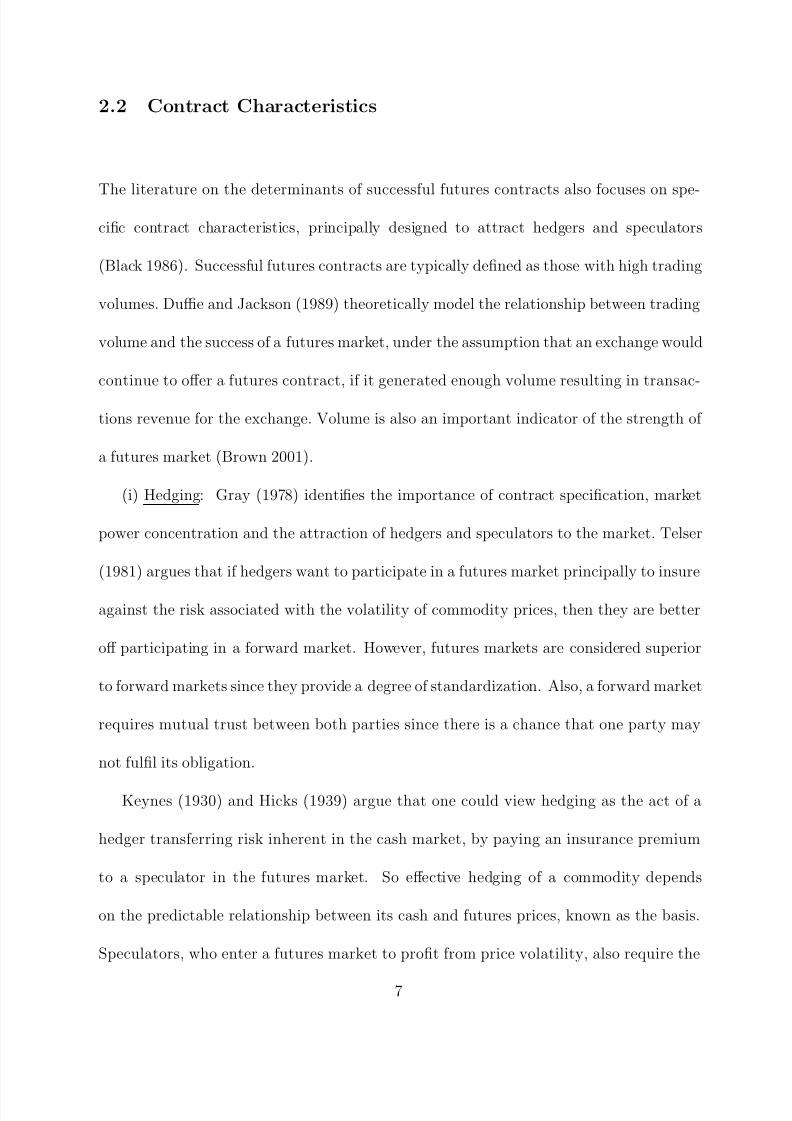
consumption was only 0.7 pounds per capita Rogers(1998). Beef has traditionally been

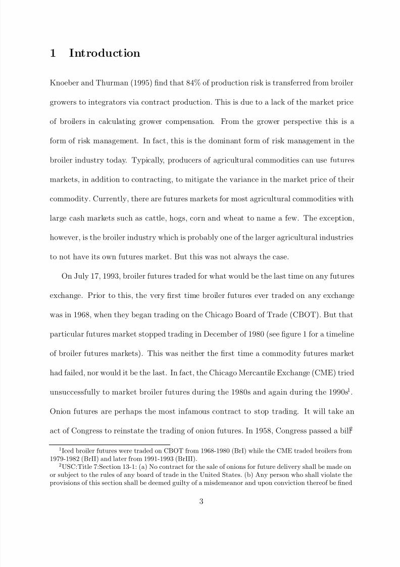
the most consumed meat on a per-capita basis. Figure 2 displays per-capita beef and

broiler consumption over the last 30 years. From figure 2 it can be noted that per-capita

broiler consumption overtook per-capita beef consumption around 1993. For 2003 the per-

capita consumption of broilers and beef were 76 pounds and 65.2 pounds, respectively9.

But one needs to realize that at the retail level beef is sold with bone and fat trimmed

from the meat prior to sale, whereas broilers are sold with most of the product discarded

as waste after the retail sale. So when compared on a boneless-weight basis, beef is still

8The term New York dressed indicates that feathers have been removed from the broilers, but nofurther processing has taken place (Bailey 1969) .

9Source: USDA Poultry Yearbook.

9



Year

l b s p e r c a p i t a

Per Capita consumption and Real Prices: Broilers and Beef

1970 1975 1980 1985 1990 199520

30

40

50

60

70

80

90

100

110

120

c e n t s / l b (

r e a l p )

50

100

150

200

250

300

350

Beef P

Broilers P

Broiler cons

Beef cons

Figure 2: Per Capita Consumption and Real Prices: Broilers and Beef

Source: 2000 USDA Poultry Yearbook

consumed more than broilers, 62 pounds per-capita to 53.2 pounds per-capita for 200310.

While declining real prices were a major contributor to increases in consumption of both

beef and broilers (figure 2), the perception of chicken as a healthy alternative to red meat

may have further increased relative broiler consumption. In 2001, 42.45 billion pounds of

broiler meat were produced at a value of $16.69 billion compared to 42.37 billion pounds

of beef valued at $29.27 billion (USDA 2001).

A shift occurred in the industry when production switched from seasonal to year-

round. This shift was a major contributor to the dramatic increase in the production

10Source: http://www.cattlefax.com

10



of broilers from 1945 when 1.11 billion pounds of broiler meat and 19.5 billion pounds

of beef were produced. Finally there have also been vast improvements in production

efficiency over the last 75 years. In 1930 it took an average of 14 weeks and 5 pounds of

feed per liveweight pound to get a broiler to market. In 2000, it took only 7 weeks and 2

pounds of feed per liveweight pound to get the average broiler to market11 (Lacy 2001).

In contrast the beef production cycle is much longer, taking six to eight months for cattle

to be market-ready.

3.2 Marketing

The process of price determination also varies between the live cattle and broiler markets.

In the wholesale broiler market, price determination is fairly informal. On Fridays of each

week, and sometimes on Thursdays and on rare Wednesdays, broiler suppliers negotiate

with buyers as to the quantity and price of broilers to be delivered the following week.

This negotiation is generally conducted over the phone between buyers and producers and

occurs in major cities and regions. All cash markets are thus regional. The twelve-city

market price is a weighted average spot market price, in lieu of an actual cash market.

Of course, both producers and buyers still use supply and demand factors to form price

expectations.

Price determination in the cattle market is a little less informal. Weekly cattle auctions

held across the Mid-West are still the basis for cattle cash market price determination.

The ‘national’ cash price for live cattle, as provided by the USDA, is a weighted average

11There have been improvements in both feed conversion, from an average of 5.0 to 2.0, as well asaverage liveweight from 2.0 pounds to 5.1 pounds.

11



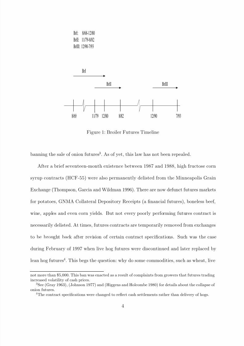
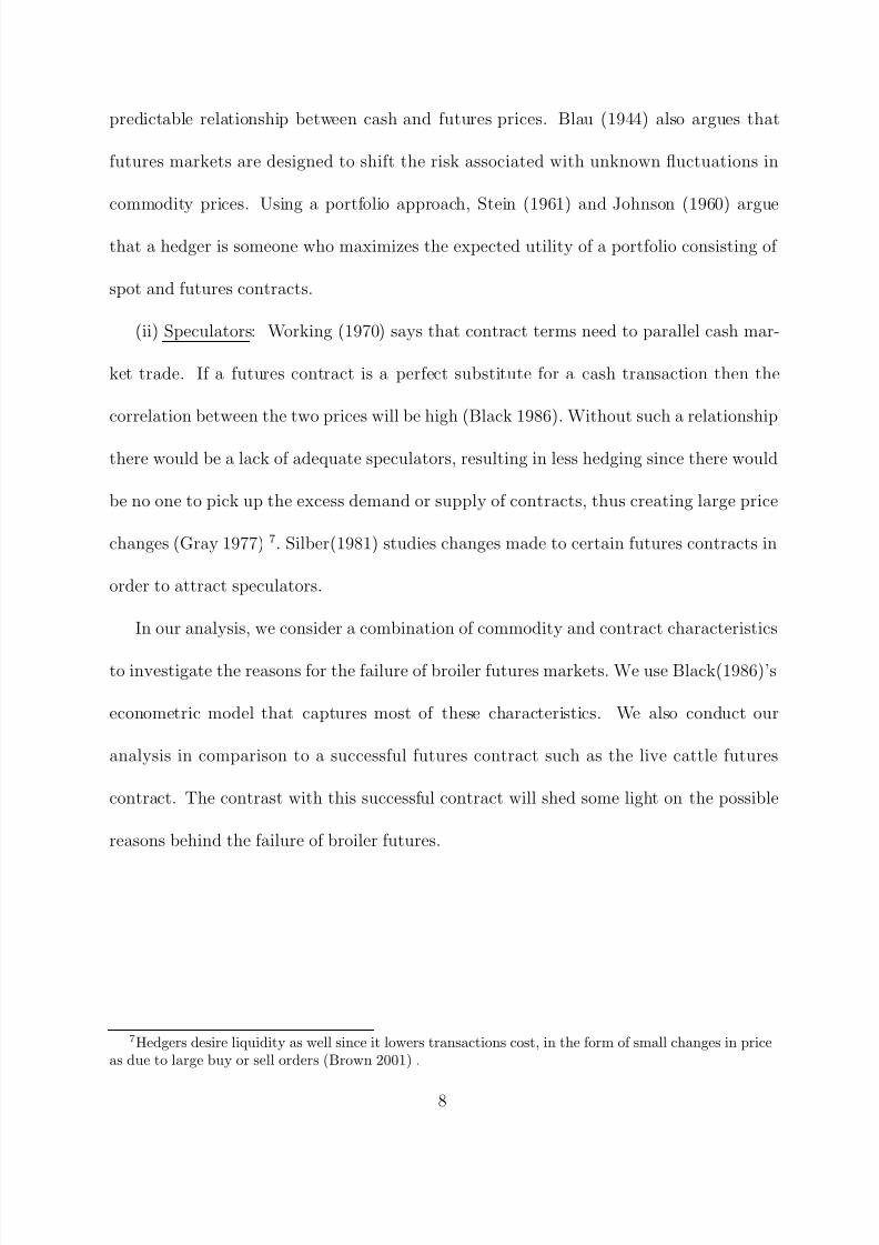
Con Agra9%

Figure 3: Market Share in Broiler Industry, 2001Source: Watt Poultry USA

of auction prices from five major beef producing states.

3.3 Current Industry Profile

In 1935 the top four broiler companies produced 30% of the industry’s output (CR4

ratio). Twenty years later they were responsible for 32% of the output (Rogers 1998).

Figure 3 provides a breakdown of the market shares of the top ten broiler producers as of

2001. These top ten companies combined to produce 80% of the industry output. Table

1 provides concentration ratios for the broiler industry for 2001. As shown in Table 2,

12



Table 1: Concentration Ratios in Broiler Industry, 2001No. of Companies % of total output

Top 4 48%Top 8 66%

Top 10 80%Top 20 90%

Source: USDA (2001)

CR4 concentration ratios have increased in the hog, cattle, turkey and poultry industries

over the last 40 years. As of 1997, of the selected commodities from Table 2, the cattle

industry had the highest CR4 concentration ratio at 71%, while broilers had the lowest,

41%. Another difference between the broiler and beef industries is in their methods of

production. While over 90% of broilers are grown under contract, only 30% of cattle are

similarly raised. The broiler industry is vertically integrated such that integrators own all

aspects of production, whereas the majority of the cattle industry is fairly independent.

Sixty-five percent of live cattle purchased by beef packers are done so at live cattle auctions

(Lawrence, Schroeder and Hayenga 2001). Processors purchase live cattle mostly from

numerous independent feedlot operators.

3.4 Broiler Futures I: 1968 - 1980 (BrI)

Given the informal nature of wholesale broiler price determination, it is not uncommon

at times for prices to fluctuate in immediate response to demand and/or supply shocks.

Towards the latter half of 1966, broiler prices were 21 cents per pound, much below the

annual average (Bailey 1969). Due to a supply shortage, the price had increased roughly

33% to 28 cents by February 1967. At the time a report commissioned by the CBOT

indicated that in the 52 week period preceding June 1968, weekly broiler prices had

13



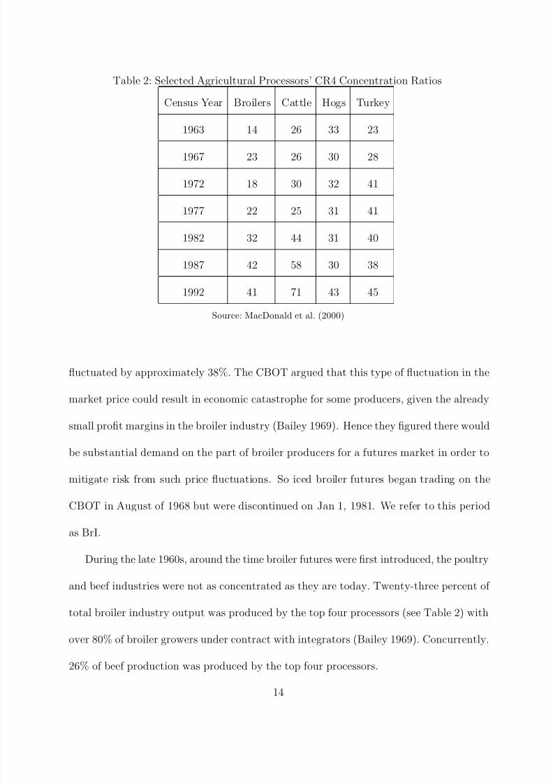
Table 2: Selected Agricultural Processors’ CR4 Concentration Ratios

Census Year Broilers Cattle Hogs Turkey

1963 14 26 33 23

1967 23 26 30 28

1972 18 30 32 41

1977 22 25 31 41

1982 32 44 31 40

1987 42 58 30 38

1992 41 71 43 45

Source: MacDonald et al. (2000)

fluctuated by approximately 38%. The CBOT argued that this type of fluctuation in the

market price could result in economic catastrophe for some producers, given the already

small profit margins in the broiler industry (Bailey 1969). Hence they figured there would

be substantial demand on the part of broiler producers for a futures market in order to

mitigate risk from such price fluctuations. So iced broiler futures began trading on the

CBOT in August of 1968 but were discontinued on Jan 1, 1981. We refer to this period

as BrI.

During the late 1960s, around the time broiler futures were first introduced, the poultry

and beef industries were not as concentrated as they are today. Twenty-three percent of

total broiler industry output was produced by the top four processors (see Table 2) with

over 80% of broiler growers under contract with integrators (Bailey 1969). Concurrently,

26% of beef production was produced by the top four processors.

14



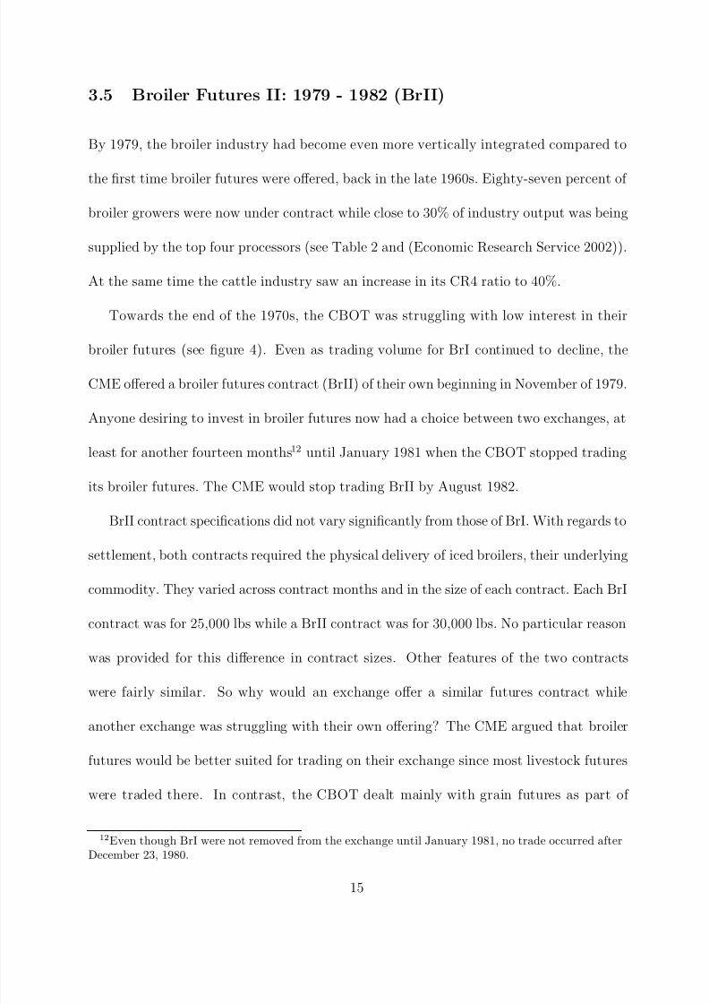
3.5 Broiler Futures II: 1979 - 1982 (BrII)

By 1979, the broiler industry had become even more vertically integrated compared to

the first time broiler futures were offered, back in the late 1960s. Eighty-seven percent of

broiler growers were now under contract while close to 30% of industry output was being

supplied by the top four processors (see Table 2 and (Economic Research Service 2002)).

At the same time the cattle industry saw an increase in its CR4 ratio to 40%.

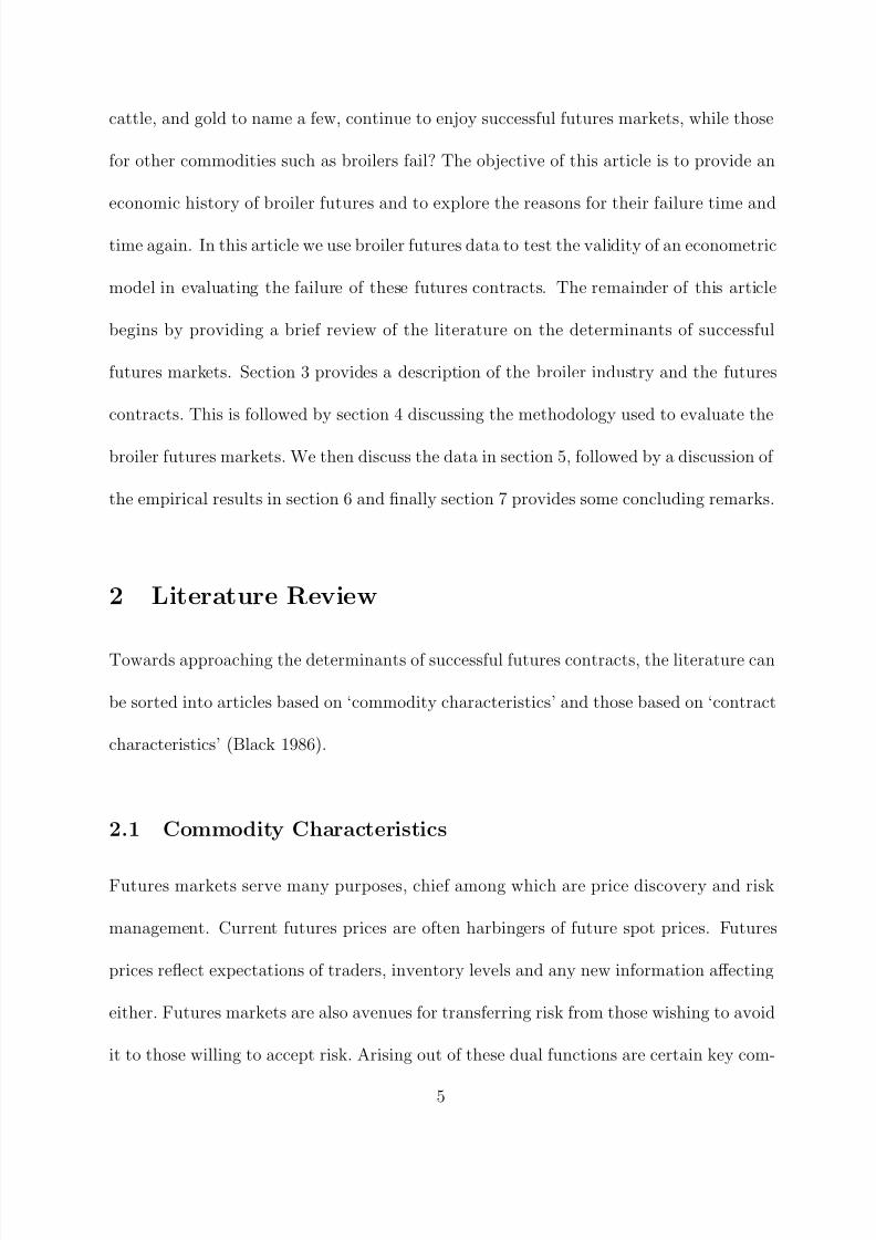
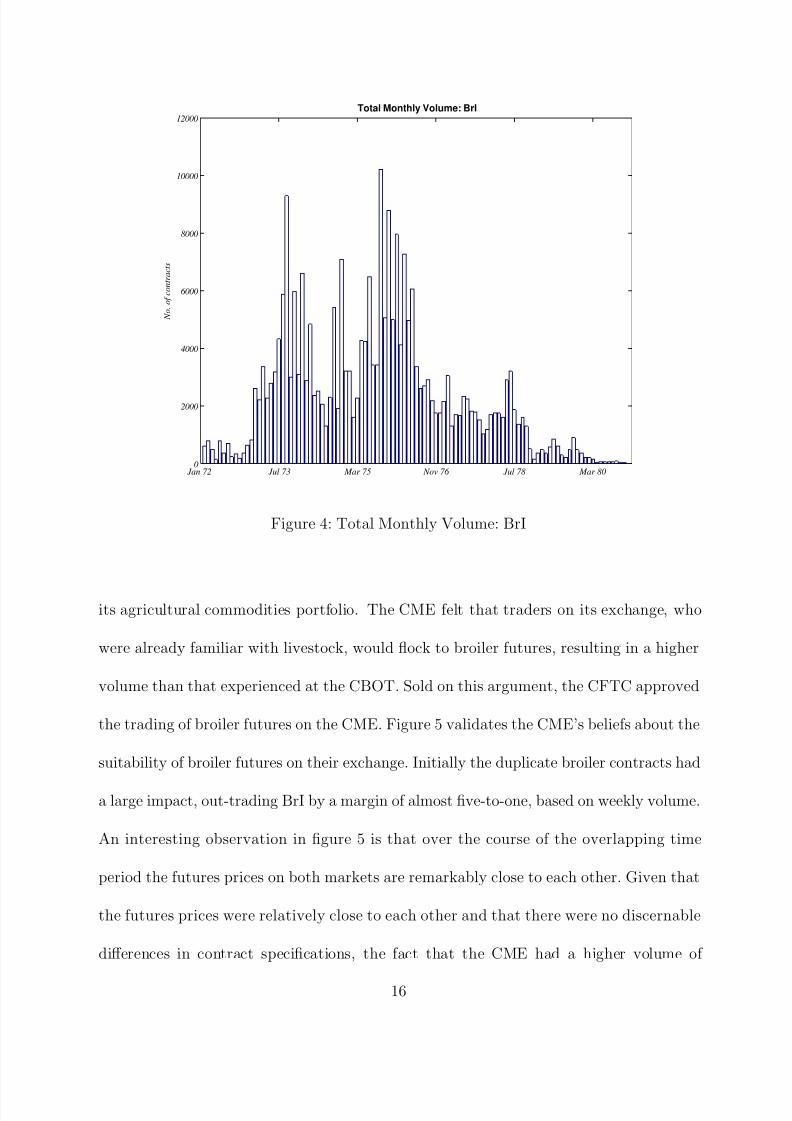
Towards the end of the 1970s, the CBOT was struggling with low interest in their

broiler futures (see figure 4). Even as trading volume for BrI continued to decline, the

CME offered a broiler futures contract (BrII) of their own beginning in November of 1979.

Anyone desiring to invest in broiler futures now had a choice between two exchanges, at

least for another fourteen months12 until January 1981 when the CBOT stopped trading

its broiler futures. The CME would stop trading BrII by August 1982.

BrII contract specifications did not vary significantly from those of BrI. With regards to

settlement, both contracts required the physical delivery of iced broilers, their underlying

commodity. They varied across contract months and in the size of each contract. Each BrI

contract was for 25,000 lbs while a BrII contract was for 30,000 lbs. No particular reason

was provided for this difference in contract sizes. Other features of the two contracts

were fairly similar. So why would an exchange offer a similar futures contract while

another exchange was struggling with their own offering? The CME argued that broiler

futures would be better suited for trading on their exchange since most livestock futures

were traded there. In contrast, the CBOT dealt mainly with grain futures as part of

12Even though BrI were not removed from the exchange until January 1981, no trade occurred afterDecember 23, 1980.

15



Jan 72 Jul 73 Mar 75 Nov 76 Jul 78 Mar 800

2000

4000

6000

8000

10000

12000

Total Monthly Volume: BrI

N o . o f c o n t r a c t s

Figure 4: Total Monthly Volume: BrI

its agricultural commodities portfolio. The CME felt that traders on its exchange, who

were already familiar with livestock, would flock to broiler futures, resulting in a higher

volume than that experienced at the CBOT. Sold on this argument, the CFTC approved

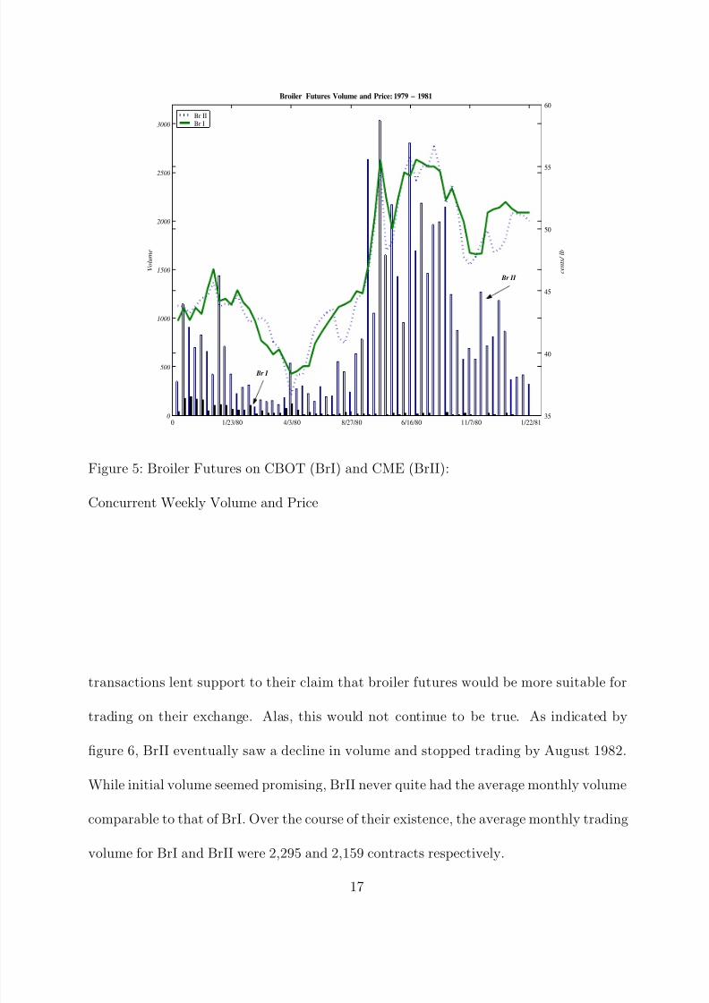
the trading of broiler futures on the CME. Figure 5 validates the CME’s beliefs about the

suitability of broiler futures on their exchange. Initially the duplicate broiler contracts had

a large impact, out-trading BrI by a margin of almost five-to-one, based on weekly volume.

An interesting observation in figure 5 is that over the course of the overlapping time

period the futures prices on both markets are remarkably close to each other. Given that

the futures prices were relatively close to each other and that there were no discernable

differences in contract specifications, the fact that the CME had a higher volume of

16



V o l u m e

0

500

1000

1500

2000

2500

3000

Broiler Futures Volume and Price: 1979 − 1981

c e n t s / l b

0 1/23/80 4/3/80 8/27/80 6/16/80 11/7/80 1/22/81

35

40

45

50

55

60

Br II

Br I

Br II

Br I

Figure 5: Broiler Futures on CBOT (BrI) and CME (BrII):

Concurrent Weekly Volume and Price

transactions lent support to their claim that broiler futures would be more suitable for

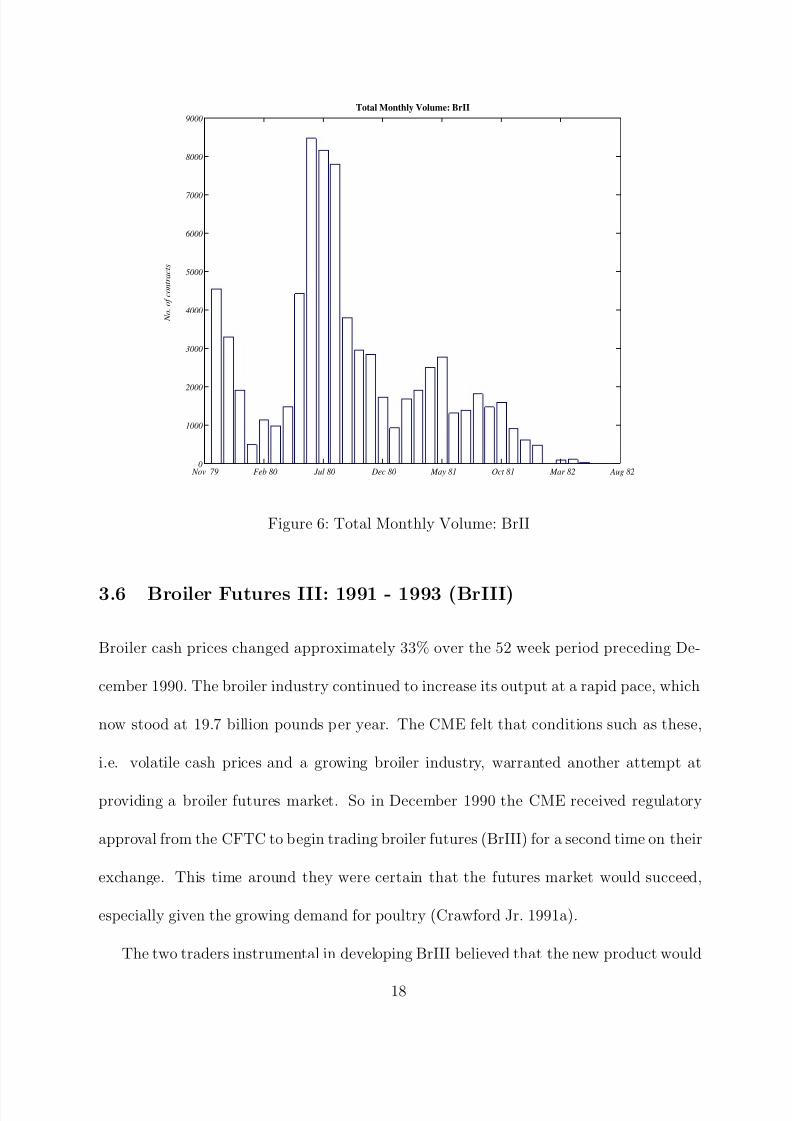
trading on their exchange. Alas, this would not continue to be true. As indicated by

figure 6, BrII eventually saw a decline in volume and stopped trading by August 1982.

While initial volume seemed promising, BrII never quite had the average monthly volume

comparable to that of BrI. Over the course of their existence, the average monthly trading

volume for BrI and BrII were 2,295 and 2,159 contracts respectively.

17



Nov 79 Feb 80 Jul 80 Dec 80 May 81 Oct 81 Mar 82 Aug 820

1000

2000

3000

4000

5000

6000

7000

8000

9000


Total Monthly Volume: BrII

Figure 6: Total Monthly Volume: BrII

3.6 Broiler Futures III: 1991 - 1993 (BrIII)

Broiler cash prices changed approximately 33% over the 52 week period preceding De-

cember 1990. The broiler industry continued to increase its output at a rapid pace, which

now stood at 19.7 billion pounds per year. The CME felt that conditions such as these,

i.e. volatile cash prices and a growing broiler industry, warranted another attempt at

providing a broiler futures market. So in December 1990 the CME received regulatory

approval from the CFTC to begin trading broiler futures (BrIII) for a second time on their

exchange. This time around they were certain that the futures market would succeed,

especially given the growing demand for poultry (Crawford Jr. 1991a).

The two traders instrumental in developing BrIII believed that the new product would

18



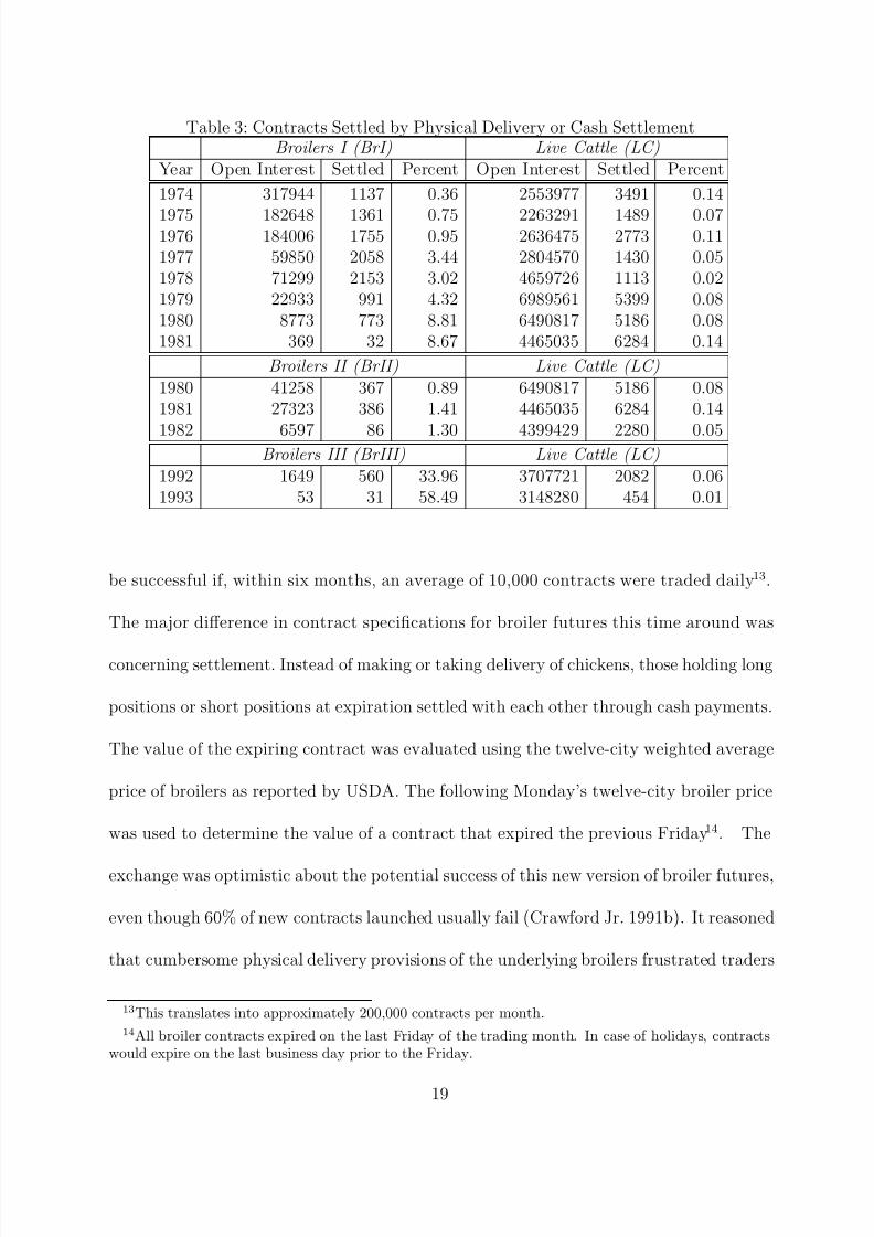
Table 3: Contracts Settled by Physical Delivery or Cash SettlementBroilers I (BrI) Live Cattle (LC)

Year Open Interest Settled Percent Open Interest Settled Percent

1974 317944 1137 0.36 2553977 3491 0.14

1975 182648 1361 0.75 2263291 1489 0.071976 184006 1755 0.95 2636475 2773 0.111977 59850 2058 3.44 2804570 1430 0.051978 71299 2153 3.02 4659726 1113 0.021979 22933 991 4.32 6989561 5399 0.081980 8773 773 8.81 6490817 5186 0.081981 369 32 8.67 4465035 6284 0.14

Broilers II (BrII) Live Cattle (LC)1980 41258 367 0.89 6490817 5186 0.081981 27323 386 1.41 4465035 6284 0.14

1982 6597 86 1.30 4399429 2280 0.05Broilers III (BrIII) Live Cattle (LC)

1992 1649 560 33.96 3707721 2082 0.061993 53 31 58.49 3148280 454 0.01

be successful if, within six months, an average of 10,000 contracts were traded daily 13.

The major difference in contract specifications for broiler futures this time around was

concerning settlement. Instead of making or taking delivery of chickens, those holding long

positions or short positions at expiration settled with each other through cash payments.

The value of the expiring contract was evaluated using the twelve-city weighted average

price of broilers as reported by USDA. The following Monday’s twelve-city broiler price

was used to determine the value of a contract that expired the previous Friday14. The

exchange was optimistic about the potential success of this new version of broiler futures,

even though 60% of new contracts launched usually fail (Crawford Jr. 1991b). It reasoned

that cumbersome physical delivery provisions of the underlying broilers frustrated traders

13This translates into approximately 200,000 contracts per month.14All broiler contracts expired on the last Friday of the trading month. In case of holidays, contracts

would expire on the last business day prior to the Friday.

19



and had led to the demise of previous futures (Dow Jones News Service 1990). Table

Feb 91 May 91 Oct 91 Mar 92 Jan 92 Jun 92 Feb 910

200

400

600

800

1000

1200

1400

Total Monthly Volume: BrIII


Figure 7: Total Monthly Volume: BrIII

3 shows the open interest15 along with the number of contracts settled via delivery for

broiler and live cattle futures16. Cattle futures data is offered for comparison of broiler

futures with an exceptionally successful futures contract.

If a contract is open at expiration, the holder of that contract must make or take

delivery of the underlying commodity. Two to four percent of most futures contracts are

settled by physical delivery. Traders, especially those who speculate, would rather offset

15Open Interest is the total number of futures contracts, either long or short in a delivery month ormarket, that have been entered into and not yet liquidated by an offsetting transaction or fulfilled bydelivery. At the start of trading of a particular futures contract month, the open interest is zero. Thischanges when a new buyer buys from a new seller or an existing long sells to an existing short, or vice-versa. It remains unchanged if a new buyer buys from an existing long or a new seller sells to an existingshort (Schwager 1984).

16Table 3 only displays values for years when data was available. Missing years do not detract fromthe general trend indicated by the table.

20



their positions prior to expiration than be forced to make or take physical delivery. A

high percentage of settlement through physical delivery or cash settlement implies one of

two things: (i) either the traders purchased contracts with the expressed intent of holding

them to maturity; (ii) or they could not find off-setting trades prior to expiration. On

average less than one quarter of one percent of cattle futures were settled by physical

delivery while more than 3% of broiler futures were settled by physical delivery in a

majority of the years that BrI contracts were traded. Even during BrII, less than the

typical amount of contracts were settled by physical delivery. So the CME’s reasoning

that physical delivery led to the demise of BrI and BrII does not seem to be supported.

In fact, during BrIII, over a third of the contracts in the first year and over half in the

second year were cash settled due to lack of a liquid market.

Two large potential hedgers, Tyson Foods and McDonald’s Corporation, expressed

reluctance to use broiler futures (Kilman 1990). McDonald’s did not have a need to

hedge since they had supply arrangements with processors and Tyson was simply not

interested17. But the number two processor, Con-Agra and another fast food chain, KFC

expressed support for broiler futures (Kilman 1990). Other reasons offered for previous

failures were that processors had little use for the type of broilers18 specified by the

contract and there were too few delivery points (Kilman 1990). With BrIII, this problem

was eliminated since settlement was not based on physical delivery but rather on cash-

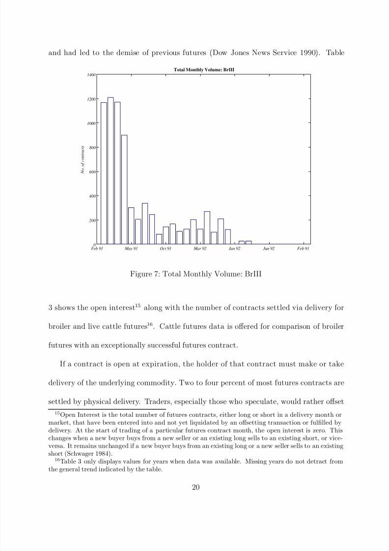
settlement. Even with these alterations to contract specifications, BrIII failed to avoid

the fate of its predecessors. For much of 1993, BrIII had single-digit volume (see figure

17In an interview one Tyson executive implied that hedging does not necessarily save a company frombankruptcy (Crawford Jr. 1991a).

18Contract settlement called for delivery of dressed, ready-to-cook, USDA Grade A broilers. Theaverage weight varied across BrI and BrII. The actual type of broiler required varies by firm.

21



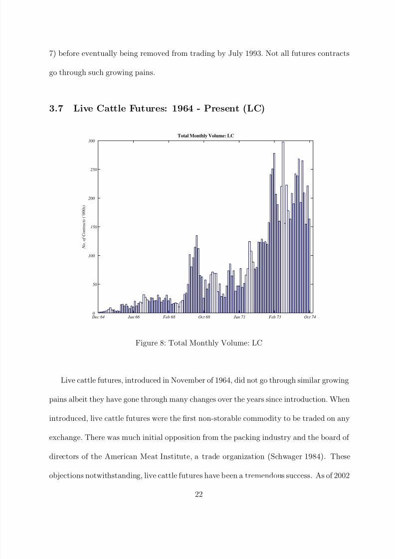
7) before eventually being removed from trading by July 1993. Not all futures contracts

go through such growing pains.

3.7 Live Cattle Futures: 1964 - Present (LC)

Dec 64 Jun 66 Feb 68 Oct 69 Jun 71 Feb 73 Oct 740

50

100

150

200

250

300

Total Monthly Volume: LC

N o . o f C o n t r a c t s ( ’ 0 0 0 s )

Figure 8: Total Monthly Volume: LC

Live cattle futures, introduced in November of 1964, did not go through similar growing

pains albeit they have gone through many changes over the years since introduction. When

introduced, live cattle futures were the first non-storable commodity to be traded on any

exchange. There was much initial opposition from the packing industry and the board of

directors of the American Meat Institute, a trade organization (Schwager 1984). These

objections notwithstanding, live cattle futures have been a tremendous success. As of 2002

22



average daily volume was approximately 12,000 contracts with an average open interest

of 103,000 contracts. By every measure live cattle futures have been successfully trading

for the last 40 years, while broiler futures traded for a combined total of 20 years during

the last 40 years. The most recent offering of broiler futures had the shortest tenure of

just under 3 years. Why was the development of a successful broiler futures market so

difficult? We now turn to the methodology that will be used in answering this question.

4 Methodology

In order to probe the reasons behind the broiler futures failures we need to consider both

the commodity characteristics and contract characteristics of futures as is common in the

literature. To recap, the commodity characteristics considered important for the existence

of successful contracts are: (i) a commodity which cannot be identified by any particular

brand (homogenous product), (ii) a commodity capable of being graded and standardized,

(iii) easily available public information regarding the commodity, (iv) a large cash market,

(v) significant variability in the cash price. Contract characteristics considered essential

to have successful contracts deal with attracting substantial hedgers and speculators and

the effectiveness of the contract as a tool for hedging.

Both broilers and cattle meet the first few commodity characteristics. Consumers do

not identify with a particular brand of either chicken or beef. Also, both commodities

are easily graded and standardized. The USDA inspects and grades poultry and cattle

as to their quality at the time of slaughter. While these characteristics are necessary

for successful contracts, they are not sufficient. A tractable model, which captures both

23



necessary and sufficient variables in predicting the success/ failure of futures is needed.

Black (1986) uses such a model.

4.1 The Model

The model as stated in Black (1986) is:

ln V olumei = ln β 0 + β 1 ln V ari + β 2 ln RRi + β 3 ln CLIQi + β 4 ln SIZE i + i (1)

where V olumei is the average monthly19 volume of futures contract i; β 0 is the constant;

V ari is commodity i’s cash price variability; RRi is the residual risk ratio defined as

follows:

RRi = residual riskcross

residual riskown=

V ar[R∗

c ]V ar[U ]

V ar[R∗

o]V ar[U ]

(2)

where ‘residual riskcross’ and ‘residual riskown’ are the risk remaining in a portfolio con-

taining a cross-hedge20 and a portfolio containing an own-hedge respectively. V ar[R∗

c ] is

the variance of a hedged portfolio containing the cash commodity and related futures,

V ar[R∗

o] is the variance of a hedged portfolio containing the cash commodity and its own

futures, and V ar[U ] is the variance of the unhedged portfolio. This comes from Edering-

ton (1979) which shows that the R2 from regressing change in cash prices onto change in

futures prices is R2 = 1− V ar[R∗]V ar[U ]

. The residual risk then is 1−R2 = V ar[R∗][V ar[U ]

, leading to the

comparison between own-hedged and cross-hedged portfolios as represented by equation

(2). CLIQi is the monthly volume in the cross futures market and SIZE i is the total

size of the cash market, measured in terms of number of contracts per month.

19Black (1986) uses daily volume.20A cross-hedge is taking a position in a related futures contract, when a futures contract does not

exist in the cash commodity.

24



In this chapter, we will explain the reasons for the failure of broiler futures by testing

the validity of equation 1 using broiler futures and cattle futures data. We now discuss

each variable in detail to hypothesize their relationship with the dependant variable,

V olume.

4.2 Volume

Let us first consider the futures exchange itself. A futures exchange is a non-profit,21

member-owned22 institution that facilitates the exchange of futures contracts. Under

its organizational profile, the CBOT states its principal role is “. . . to provide contract

markets for its members and customers . . . ”23. The implied secondary role is to “. . . also

provide opportunities for risk management for users who include farmers, corporations,

small businesses and others”24. So the primary goal of an exchange is to offer any contract

which would result in high volume. High volume for the exchange results in higher

commissions and transactions fees for its members. While the exchange itself may be a

not-for-profit organization, its members nonetheless are for-profit institutions. So it can be

argued that contracts are considered failures, and subsequently delisted by the exchange,

if they do not generate enough volume, as designated by the particular exchange.

What is considered a ’successful’ level of volume may vary across exchanges25. So, we

21In 1999 the CBOT, the largest futures exchange in the US, considered a proposal to restructure itself into a for-profit corporation, although this change has not yet taken place.

22Only members or their representatives are allowed to trade on exchanges. Member status is acquiredby purchasing a ’seat’ on the exchange through a bid and ask system. As of Dec 12, 2003 a full membershipon the CBOT sold for $520,000 (http://www.cbot.com). The price of an exchange seat is viewed bysome as an indication of the exchange’s ability to attract business that generally rises during times of commodity-price volatility and falls during low trading volume on the exchange (WSJ 1980).

23Under “organizational profile” at http://www.cbot.com24ibid.25Typically, all new contracts offered on the exchange go through a ‘probationary’ phase. On the CME

the end of the probationary phase known as ‘the Initial Termination Date’ for new products, is “. . . the

25



turn to the literature for some volume threshold values. Sandor (1973) uses an average

annual volume of 1,000 contracts as the threshold to determine a contract’s success, while

Silber (1981) uses an annual volume of 10,000 contracts as a measure of success. Black

(1986) uses a threshold of 1,000 contracts traded daily as an indicator of contract success 26.

Never during their existence did broiler futures average such volume levels (see figures 4,

6 and 7), hence they were removed from trading. But since our objective is to explore

the reasons for broiler future failures and not to predict whether or not they will fail,

we are not particularly concerned with a threshold value for our dependent variable. We

are more concerned with the results of estimating equation 1 in order to check if the

parameters support theoretical predictions.

4.3 Price Variability (Var)

As previously mentioned, without the presence of hedgers, there would be no futures

markets. Variability in the cash price of a given commodity is the main reason hedgers

turn to futures markets. So it would follow that the higher the cash price variability, the

higher the trading volume, such that ∂V olumei∂V ari

> 0.

4.4 Residual Risk (RR) (Effective Hedging )

An ideal hedge is one where the underlying futures commodity exactly matches the cash

commodity. Even though not all commodities have a corresponding futures market, one

latter of (1) two years after the date that trading in such products starts or (2) the first day of the monthafter volume of trading for that product (futures and options combined) averaged at least 1,000 contractsper day . . . ” (CME 2003).

26Generally speaking, a market with average daily volume of 1,000 contracts is considered successful(Schwager 1984)

26



can still reduce output price risk via the futures market with cross-hedging. This can be an

effective risk management tool if there is a dependable price relationship between the cash

commodity and the related commodity futures contract (Black 1986). Compared to an

own-hedge (where the cash commodity being hedged and the futures contract underlying

commodity are the same), the cross-hedge is generally characterized as having higher

residual risk. Residual risk, as defined earlier, is the risk remaining in the hedged position

compared to a perfect hedge where all risk is eliminated. For example, if the R2 from the

cross-hedge regression is 0.244 and the R2 from the own-hedge regression is 0.468, the

RR variable is calculated to be 1.4211.27 If on the other hand, R2 from the cross-hedge

is 0.75 and from the own-hedge is 0.45 then RR will equal 0.4545. The closer is R2 to

one, the more effective is the hedge. Given the formulation for RR, the more effective the

own-hedge greater is RR. If the own-hedge is more effective than the cross-hedge, hedgers

would prefer their own commodity futures contract. So the relationship between V olumei

and RRi should be ∂V olumei∂RRi

> 0.

4.5 Liquidity in the cross futures market (CLIQ)

If the cross futures market can be used as a more effective hedging tool, traders would

rather be in that particular market. Occasionally even if a cross-hedge has a lower R2 (is

less effective) traders might flock to its markets due to increased liquidity. If there are

significantly more transactions that take place in the cross futures market, the associated

liquidity costs will be lower relative to the own futures market. Liquid markets are

markets where selling and buying can be accomplished with minimal effect on price. While

27RR = 1−0.244

1−0.468 = 1.4211

27



volatility in a futures market would attract some traders, the lack of liquidity would keep

them away since it may be difficult for them to find off-setting transactions when needed.

This being the case one would expect the cross futures volume to be inversely related to

the volume of the own futures market, ∂V olumei∂CLIQi

< 0.

4.6 Size of the cash market (SIZE)

The obvious reason to have a large cash market is to make available a large supply of

potential hedgers. Another reason that the size of the cash market matters is because it

prevents manipulation of the market and allows for the free movement of prices (Black

1986). The hypothesized relationship between size of the cash market and volume is

∂V olumei∂SIZE i

> 0.

5 Data

Our data come primarily from three sources: the CBOT, The Wall Street Journal and

the Bridge/ CRB database. Data for BrI begins from January 1972. Futures data prior

to 1972 was unavailable and as such for the purposes of this estimation, BrI starts in

January of 1972. When we refer to BrI, we do so to the time period of 1972 – 1980. Cash

and futures prices as well as volume data for BrI come from the CBOT, while all data

pertaining to BrII come from The Wall Street Journal . Cash prices, futures prices and

volume for BrIII and live cattle (LC) come from the Bridge/ CRB database. The time

span for the LC futures covers the period from December 1964 (when LC futures were

first introduced) to Dec 1971.

28



5.1 Data Management

A monthly frequency of all variables is used in estimating equation 1. While some variables

had monthly observations, others needed to be transformed to a monthly observation in

the following manner:

Volume: The monthly volume used in the estimation is a sum of the weekly values as

stated in the databases.

Var: The standard deviation of daily cash prices for a month is used as the measure of

the price variability of that particular month.

RR: The production cycle for broilers ranges between six to eight weeks. We choose seven

weeks (thirty-five days) as the hedging horizon to calculate R2s to be used in calculating

RR. Daily changes in cash price are used for the regression of cash price changes onto

futures price changes. The sample for each such regression consists of 35 observations.

The same procedure is followed to attain futures price changes.

SIZE: Data for cash market size are from the USDA monthly poultry slaughter and

monthly cattle slaughter. The total weight at slaughter is then converted to contract

equivalents by dividing total weight by the contract size of the relevant contract. Each

broiler contract during BrI, BrII and BrIII was for 25,000 lbs, 30,000 lbs and 40,000 lbs

respectively. One LC contract is for 40,000 lbs. Market size related in terms of contracts

gives an indication of the size of potential hedgers. Poultry slaughter data prior to 1974

was either incomplete or unavailable.

For BrI a complete data set (monthly observations) was only available from 1974,

providing us with a total of 84 observations. We use the same number of observations

29



from a comparable time period for live cattle. BrII and BrIII each have a total of 33 and

29 monthly observations respectively. With the exception of BrI, all other futures either

traded or continue to trade on the CME. BrI traded on the CBOT.

Live hog futures are used as the related futures for cross hedging for both broilers and

live cattle. The time series for hog futures are from comparable time periods. Data for

live hog futures, traded on the CME, were obtained from the Bridge/ CRB dataset.

6 Empirical Analysis

Table 4 displays the expected and estimated parameter signs from regressing equation

1. For purposes of brevity only parameter signs and levels of significance are reported.

The first row of table 4, labelled ’Expected ’, lists parameter signs as predicted by theory.

The second row, labelled LC lists the estimated signs from regressing live cattle futures

data using equation 1. As predicted by theory, variables Var and SIZE have the correct

sign and are significant at the 5% level. However, RR is not significant and thus not

a source of major concern, even if the sign is opposite of that expected. On the other

hand, CLIQ is significant at the 5% level and has a sign opposite to that predicted by

theory. The positive sign on CLIQ implies that as trading volume increases in the cross

futures market (live hogs), it also leads to increased volume in the LC market. The same

significant relationship (CLIQ > 0) is found for the BrI dataset. Since other parameters

for BrI, BrII and BrIII are not significant, we are not concerned with their signs. Our

control group of successful futures, LC, did not have the desired signs. So we need to

augment (Black 1986) to arrive at a regression equation which will adequately explain the

30



live cattle futures data and help explain the broiler futures.

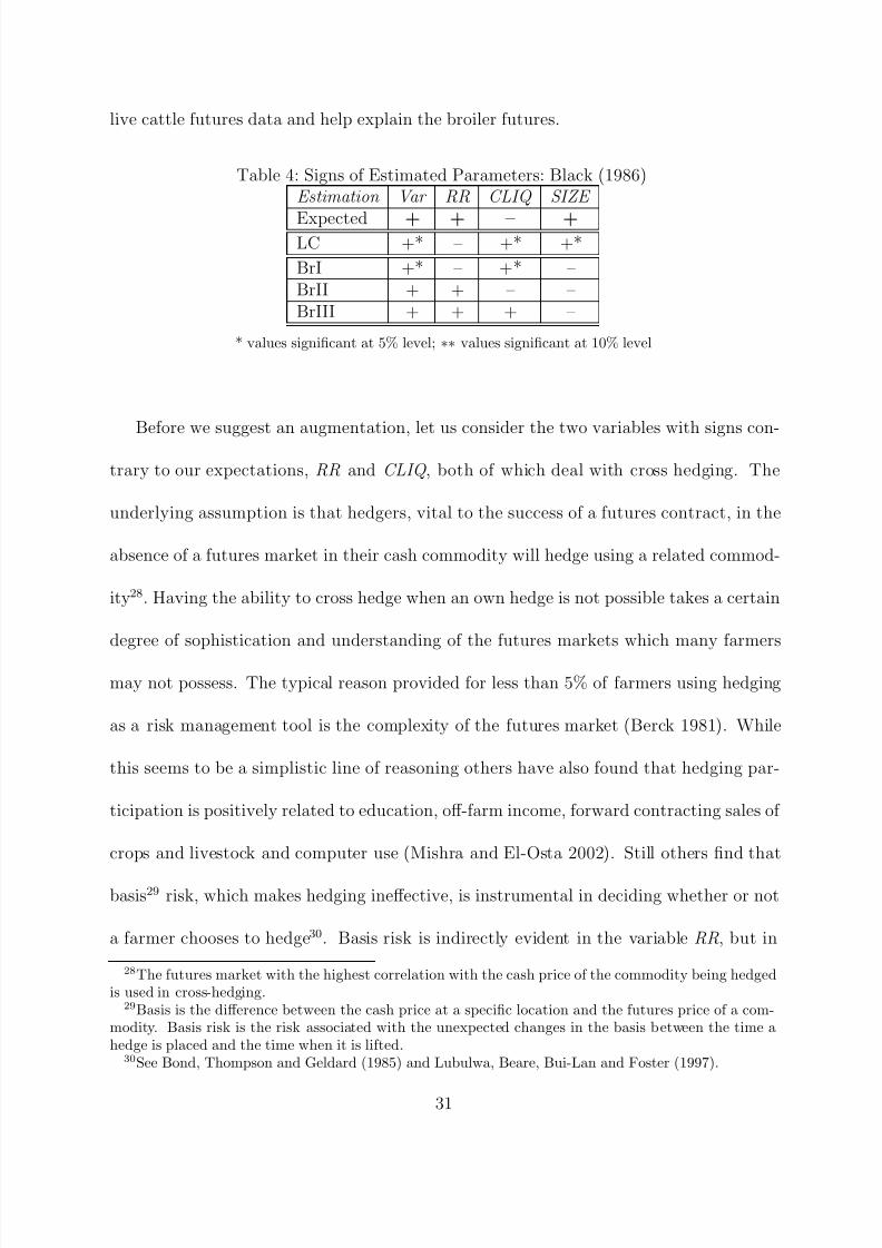
Table 4: Signs of Estimated Parameters: Black (1986)Estimation Var RR CLIQ SIZE

Expected + + – +LC +* – +* +*

BrI +* – +* –BrII + + – –BrIII + + + –

* values significant at 5% level; ∗∗ values significant at 10% level

Before we suggest an augmentation, let us consider the two variables with signs con-

trary to our expectations, RR and CLIQ , both of which deal with cross hedging. The

underlying assumption is that hedgers, vital to the success of a futures contract, in the

absence of a futures market in their cash commodity will hedge using a related commod-

ity28. Having the ability to cross hedge when an own hedge is not possible takes a certain

degree of sophistication and understanding of the futures markets which many farmers

may not possess. The typical reason provided for less than 5% of farmers using hedging

as a risk management tool is the complexity of the futures market (Berck 1981). While

this seems to be a simplistic line of reasoning others have also found that hedging par-

ticipation is positively related to education, off-farm income, forward contracting sales of

crops and livestock and computer use (Mishra and El-Osta 2002). Still others find that

basis29 risk, which makes hedging ineffective, is instrumental in deciding whether or not

a farmer chooses to hedge30. Basis risk is indirectly evident in the variable RR, but in

28The futures market with the highest correlation with the cash price of the commodity being hedgedis used in cross-hedging.

29Basis is the difference between the cash price at a specific location and the futures price of a com-modity. Basis risk is the risk associated with the unexpected changes in the basis between the time ahedge is placed and the time when it is lifted.

30See Bond, Thompson and Geldard (1985) and Lubulwa, Beare, Bui-Lan and Foster (1997).

31



order to understand the success/ failure of futures contracts, especially in the agricultural

commodities, we need to incorporate a more direct measure of the basis risk. With RR

and CLIQ not being significant, and to incorporate a more direct measure of a basis risk,

we propose the following augmented model:

ln V olumei = ln β 0 + β 1 ln V ari + β 2 ln basisi + β 3 ln SIZE i + i (3)

where basisi is the basis risk and other variables are as previously defined. If there is no

dependable relationship between the cash price and the futures price, then hedging indeed

does become ineffective. So one would expect the bigger the basis risk of a commodity,

the less the transaction volume in its futures market, ∂V olume∂basis

< 0

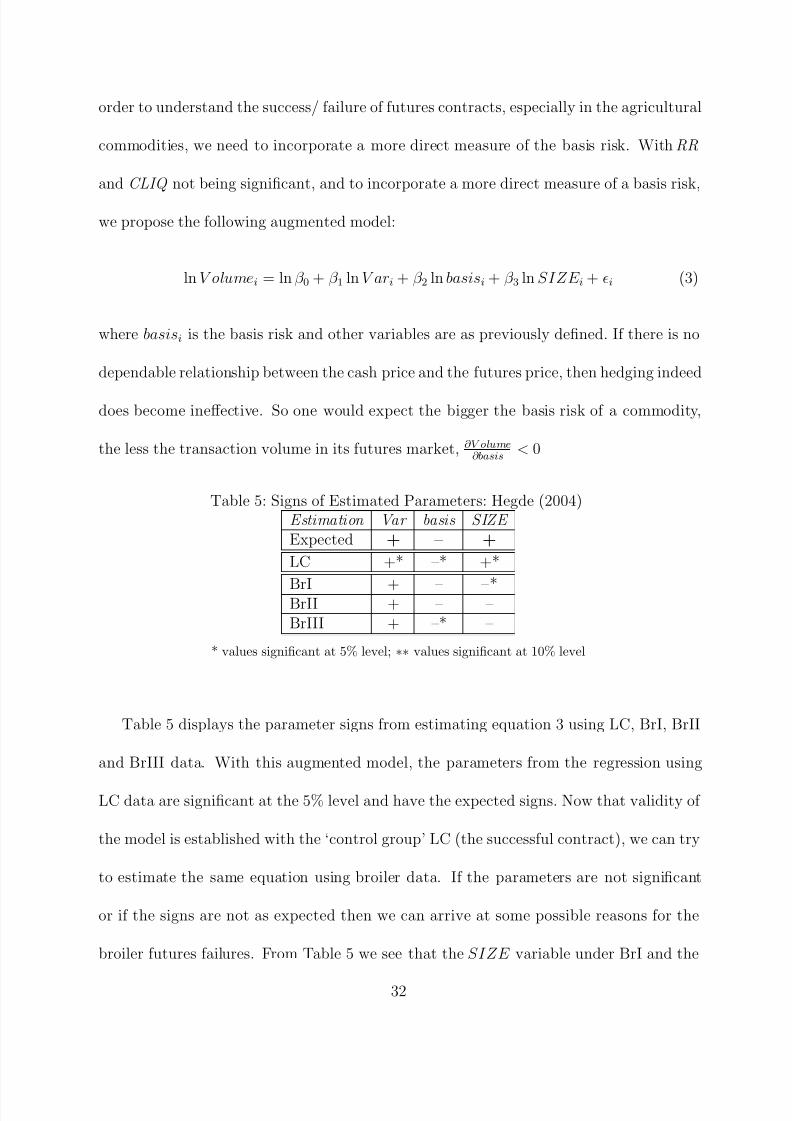
Table 5: Signs of Estimated Parameters: Hegde (2004)Estimation Var basis SIZE Expected + – +

LC +* –* +*

BrI + – –*BrII + – –BrIII + –* –

* values significant at 5% level; ∗∗ values significant at 10% level

Table 5 displays the parameter signs from estimating equation 3 using LC, BrI, BrII

and BrIII data. With this augmented model, the parameters from the regression using

LC data are significant at the 5% level and have the expected signs. Now that validity of

the model is established with the ‘control group’ LC (the successful contract), we can try

to estimate the same equation using broiler data. If the parameters are not significant

or if the signs are not as expected then we can arrive at some possible reasons for the

broiler futures failures. From Table 5 we see that the SIZE variable under BrI and the

32



basis variable under BrIII are the only significant variables. It is curious why the sign on

SIZE is negative (even if not significant). The basis variable has the correct sign, even

if it is not significant. We need to examine more closely the basis for all three futures.

In combination with that examination, we may be able to hypothesize as to the reasons

behind broiler failures.

Basis is expected to converge to zero as a contract approaches expiration. At expi-

ration, the basis is expected to be zero as the futures price and the cash price equalize.

However local basis, which is the difference between the price received by a farmer in his

region and the futures price, is not expected to equal zero at contract expiration. This

is because futures contracts require physical delivery to exchange-designated locations,

which may be different than the location of the farmer. Basis risk is defined as the unex-

pected widening or narrowing of the basis between the time a hedge position is established

and the time that it is lifted. Basis risk can result in changes to the expected price from

hedging. The hedge ratio which is a ratio of futures position to cash position for a hedger

is affected by basis risk. It is basis risk which is of interest to us, since hedging becomes

ineffective with high basis risk.

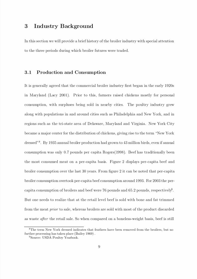
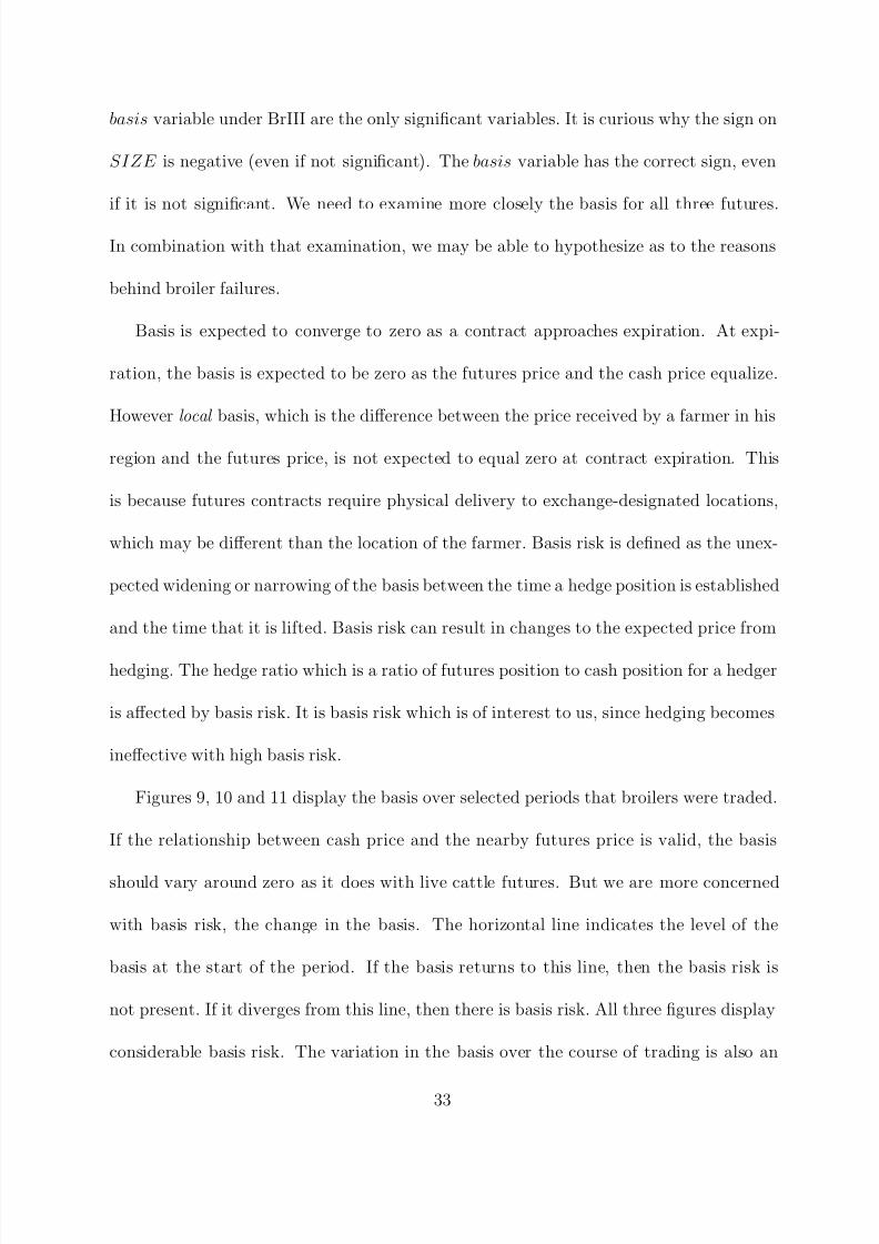
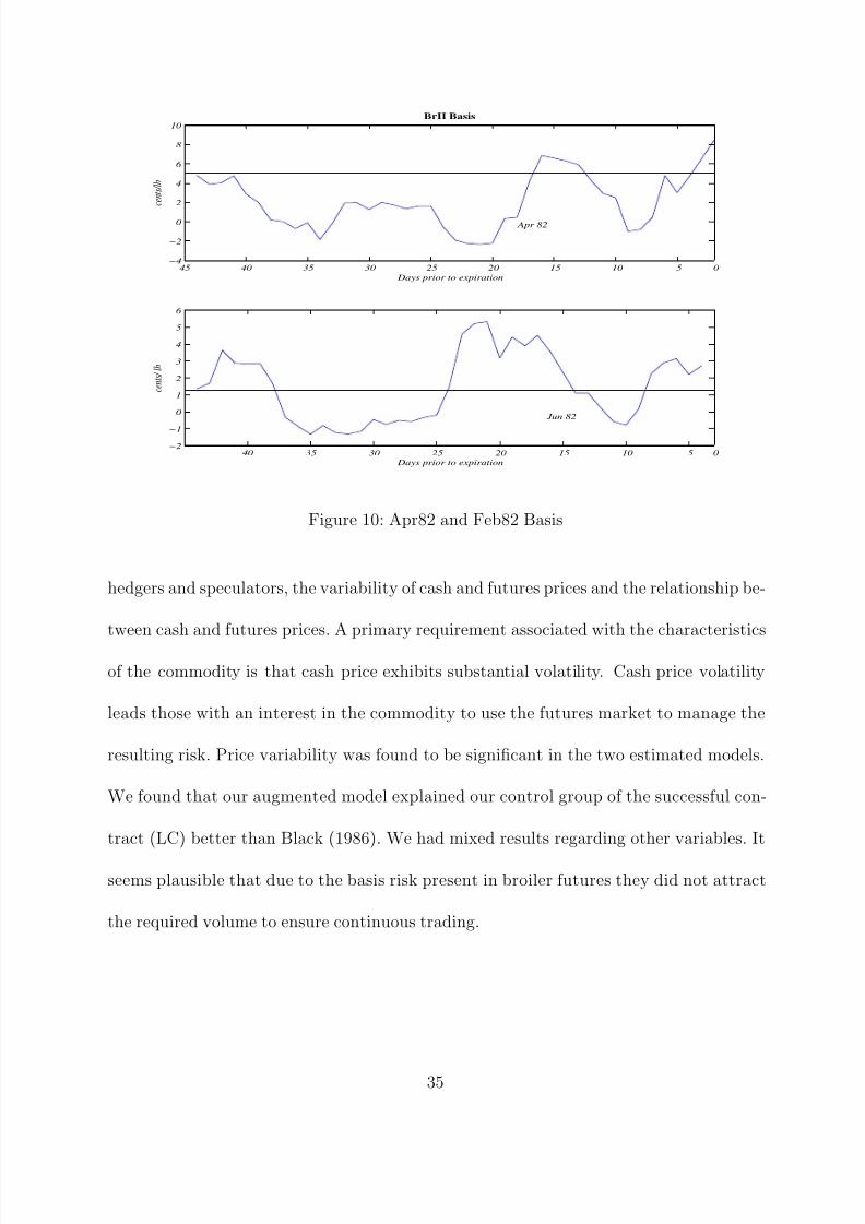
Figures 9, 10 and 11 display the basis over selected periods that broilers were traded.

If the relationship between cash price and the nearby futures price is valid, the basis

should vary around zero as it does with live cattle futures. But we are more concerned

with basis risk, the change in the basis. The horizontal line indicates the level of the

basis at the start of the period. If the basis returns to this line, then the basis risk is

not present. If it diverges from this line, then there is basis risk. All three figures display

considerable basis risk. The variation in the basis over the course of trading is also an

33



25 20 15 10 5 00

2

4

6

8

10

12

Basis for BrII futures

Days prior to expiration

c e n t s

/ l b

40 35 30 25 20 15 10 5 0−10

−5

0

5

10

15


c e n t s

/ l b

Feb 82

Dec 82

Figure 9: Dec82 and Feb82 Basis

indication of basis risk. Having a high basis risk, as demonstrated by its variance, implies

that the hedge ratio would not be close to one and in fact may be closer to zero. Given

the variance in the basis, hedging with broiler futures may not be an effective tool for risk

management. This offers yet another reason why broiler futures may have failed.

7 Conclusion

The objective of this chapter was to investigate reasons why broiler futures markets re-

peatedly collapsed over the last 40 years. Much of the literature focuses on certain char-

acteristics of either the underlying commodity or the contract itself as requirements for

successful futures contracts. In this chapter we considered a combination of both com-

modity and contract characteristics. We considered trading volume, the ability to attract

34



45 40 35 30 25 20 15 10 5 0−4

−2

0

2

4

6

8

10


c e n t s / l b

BrII Basis

40 35 30 25 20 15 10 5 0−2

−1

0

1

2

3

4

5

6


c e n t s / l b

Apr 82

Jun 82

Figure 10: Apr82 and Feb82 Basis

hedgers and speculators, the variability of cash and futures prices and the relationship be-

tween cash and futures prices. A primary requirement associated with the characteristics

of the commodity is that cash price exhibits substantial volatility. Cash price volatility

leads those with an interest in the commodity to use the futures market to manage the

resulting risk. Price variability was found to be significant in the two estimated models.

We found that our augmented model explained our control group of the successful con-

tract (LC) better than Black (1986). We had mixed results regarding other variables. It

seems plausible that due to the basis risk present in broiler futures they did not attract

the required volume to ensure continuous trading.

35



25 20 15 10 5 00

2

4

6

8

10

12


c e n t

s / l b

20 15 10 5 0−1

0

1

2

3

4

5

6

7

BrII Basis


c e n t s

/ l b

Jul 82

Aug 82

Figure 11: Jul82 and Aug82 Basis

36



References

Bailey, Fred, “Understanding The Iced Broiler Futures Market,” 1969 CRB Yearbook ,1969.

Berck, P., “Portfolio Theory and the Demand for Futures,” American Journal of Agri-cultural Economics , 1981, 64, 466–74.

Black, Deborah C., “Success and Failure of Futures Contracts Theory and EmpiricalEvidence,” Technical Report, Solomon Brothers Center for the Study of FinancialInstitutions 1986.

Blau, G., “Some Aspects of the Theory of Futures Trading,” Review of Economic Studies ,1944, 12 , 1–30.

Bond, G.E., S. R. Thompson, and J. M. Geldard, “Basis Risk and Hedging Strate-gies for Australian Wheat Exports,” Australian Journal of Agricultural Economics ,1985, 29 , 199–209.

Brown, Christine A., “The Successful Redenomination of a Futures Contract: TheCase of the Australian All Ordinaries Share Price Index Futures Contract,” Pacific-Basin Finance Journal , 2001, 9 , 47–64.

Carlton, D. W., “Futures Markets: Their Purpose, Their History, Their Growth, TheirSuccesses and Failure,” The Journal of Futures Markets , 1984, 4, 237–274.

Chicago Mercantile Exchange, “Rule Book,” http://www.cme.com 2003.

Crawford Jr., William B., “Chicken Futures Contract Aloft at Merc,” Chicago Tribune ,February 8 1991, p. 3.

, “Mixed Signals Transmitted by 3 Exchanges,” Chicago Tribune , Sept 5 1991, p. C1.

Dow Jones News Service, “Chicago Merc Gets Okay for Broiler Chicken Futures,”Wire Service Dec 21 1990.

Duffie, D. and M. O. Jackson, “Optimal Innovation of Futures Contracts,” Review of Financial Studies , 1989, 2 (3), 275–296.

Economic Research Service, “U.S. Food Marketing System, 2002,” AER 811, USDA

2002.

Ederington, Louis H., “The Hedging Performance of the New Futures Markets,” The Journal of Finance , March 1979, 34 (1), 157–170.

Garbade, Kenneth D., Securities Markets , New York, N.Y.: McGraw–Hill, 1982.

Gray, R. W, “Price Effects of a lack of Speculation,” in A.E. Peck, ed., Readings in Futures Markets, Volume 2 , Chicago: Chicago Board of Trade, 1977.

Gray, R.W., “Onions Revisited,” Journal of Farm Economics , 1963, 45 , 273–276.

37



, “Why Does Futures Trading Succeed or Fail: An Analysis of Selected Commodi-ties,” in A.E. Peck, ed., Readings in Futures Markets, Volume 3: View from the Trade , Chicago: Chicago Board of Trade, 1978.

Hicks, J. R., Value and Capital , London: Oxford University Press, 1939.

Higgens, Richard S. and Randall G. Holcombe, “The Effect of Futures Trading onPrice Variability in the Market for Onions,” Atlantic Economic Journal , July 1980,8 (2), 50–51.

Johnson, Aaron C., “Effects of Futures Trading on Price Performance in the CashOnion Market, 1930-1958,” in A.E. Peck, ed., Selected Writings on Futures Markets,Volume II , Chicago: Chicago Board of Trade, 1977, pp. 329–336.

Johnson, Leland L., “The Theory of Hedging and Speculation in Commodity Futures,”Review of Economic Studies , 1960, 27 , 139–151.

Keynes, John M., A Treatise on Money , London: Macmillan, 1930.

Kilman, Scott, “Broilers May Return to Roost at Merc,” Wall Street Journal , 1990,p. C1.

Knoeber, Charles R. and Walter N. Thurman, “Don’t Count Your Chickens . . .

Risk and Risk Shifting in the Broiler Industry,” American Journal of Agricultural Economics , August 1995, 77 , 486–496.

Lacy, Michael P., “Broiler Production - Past, Present and Future,” Bulletin, The Uni-versity of Georgia 2001.

Lawrence, J. D, T. C. Schroeder, and M. L. Hayenga, “Evolving Producer-Packer-Customer Linkages in the Beef and Pork Industries,” Review of Agricultural Eco-nomics , 2001, 23 , 370–385.

Leuthold, Raymond M., J. C. Jukus, and J.E. Cordier, The Theory and Practice of Futures Markets , Lexington, MA: Lexington Books, 1989.

Lubulwa, M., S. Beare, A. Bui-Lan, and M. Foster, “Wool Futures: Price RiskManagement for Australian Wool Growers,” Research Report 97.1, Australian Bu-reau of Agricultural and Resource Economics 1997.

MacDonald, J. M., Michael E. Ollinger, Kenneth E. Nelson, and Charles R.

Handy., “Consolidation in U.S. Meat Packing,” Report 785, ERS:USDA 2000.

Malliaris, A.G., “Futures Markets: Why are they different?,” in A.G. Malliaris, ed.,Foundations of Futures Markets: Selected Essays of A.G. Malliaris , 2000, chapter 1,pp. 8–25.

Mishra, Ashok and Hisham El-Osta, “Managing Risk in Agriculuture through Hedg-ing and Crop Insurance: What Does a National Survey Reveal?,” Agricultural Fi-nance Review , Fall 2002, 62 (2), 135–48.

38



Rogers, Richard T., “Broilers: Differentiating a Commodity,” in Larry L Deutsch, ed.,Industry Studies , Armonk, NY: M.E. Sharpe, 1998, chapter 3, pp. 65–100.

Sandor, Richard L., “Innovation by an Exchange: A Case Study of the Developmentof the Plywood Futures Contract,” The Journal of Law and Economics , April 1973,

16 (1), 119–136.

Schwager, Jack D., A Complete Guide to the Futures Market , John Wiley and Sons,1984.

Silber, W.L., “Innovation, Competition, and New Contract Design in Futures Markets,”Journal of Futures Markets , 1981, 1, 123–155.

Stein, Jerome L., “The Simultaneous Determination of Spot and Futures Prices,” Amer-ican Economic Review , 1961, 51, 1012–1025.

Telser, Lester G., “Why There are Organized Futures Markets,” The Journal of Law and Economics , 1981, 24, 1–22.

Thompson, S., P. Garcia, and L. D. Wildman, “The Demise of the High FructoseCorn Syrup Futures Contract: A Case Study,” The Journal of Futures Market , 1996,16 (6), 697–724.

USDA, “Broiler Industry Structure,” Bulletin, National Agricultural Statistical Service2002.

Working, Holbrook, “Economic Functions of Futures Markets,” in “Selected Writingsof Holbrook Working,” Chicago: CFTC, 1977, pp. 267–297.

WSJ, “Seat Prices on Futures Exchanges Drop; Turnaround Seen as Contracts Recover,”The Wall Street Journal , December 30 1980, p. 38.

Documents

An Economic History of the Failure of Broiler Futures