1

An economics study

Question: Is there a difference in the returns to education for men

and for women? If so, what is the difference?

This example is adapted from E8.1, of the recommended textbook

Introduction to Econometrics, 3rd Edition (Update), by Stock and

Watson.

We will use a variant of the CPS data. The data description may be

found by following the link:

http://wps.aw.com/wps/media/objects/3833/3925976/datasets2e/datasets/CPS04_Description.pdf

2

The variable definitions are:

ahe – average hourly earnings, in $/week.

bachelor – a dummy variable equal to 1 if the worker has a

university degree, or equal to 0 if the worker has a high school

degree.

female – a dummy variable equal to 1 if worker is female, 0

otherwise.

age – the age, in years, of the worker.

The sample size is n = 7986.

3

In order to answer the main question, we need to specify the right

population model, so that our estimators are unbiased. We will

make use of:

Polynomials

Logarithms

Interaction terms

in our efforts to get the right model. We will use t-tests, F-tests,

and adjusted R2 in order to choose between models.

We will ignore the problem of heteroskedasticity.

Regression results will be reported in a table:

4

Question number: 1 2 3 4 5 7 8 9

Dependent Variable

Dependent var.: AHE AHE log(AHE) log(AHE) log(AHE) log(AHE) log(AHE) log(AHE)

Age

Age2

log(Age)

Female×Age

Female×Age2

Bachelor×Age

Bachelor×Age2

Female

Bachelor

Female×Bachelor

Intercept

𝑅2

�̅�2

Significance at the *5% and **1% significance level.

5

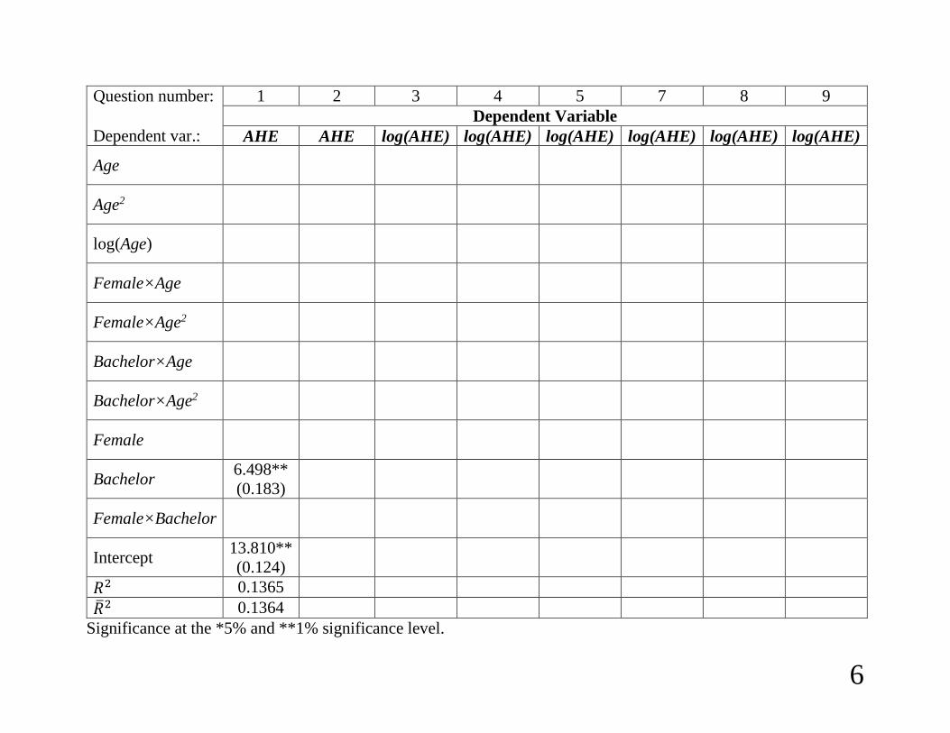
1. Regress AHE on Bachelor.

> summary(lm(ahe ~ bachelor))

Estimate Std. Error t value Pr(>|t|)

(Intercept) 13.8096 0.1235 111.85 <2e-16 ***

bachelor 6.4975 0.1829 35.53 <2e-16 ***

---

Signif. codes: 0 ‘***’ 0.001 ‘**’ 0.01 ‘*’ 0.05 ‘.’ 0.1 ‘ ’ 1

Residual standard error: 8.139 on 7984 degrees of freedom

Multiple R-squared: 0.1365, Adjusted R-squared: 0.1364

F-statistic: 1262 on 1 and 7984 DF, p-value: < 2.2e-16

6

Question number: 1 2 3 4 5 7 8 9

Dependent Variable

Dependent var.: AHE AHE log(AHE) log(AHE) log(AHE) log(AHE) log(AHE) log(AHE)

Age

Age2

log(Age)

Female×Age

Female×Age2

Bachelor×Age

Bachelor×Age2

Female

Bachelor 6.498**

(0.183)

Female×Bachelor

Intercept 13.810**

(0.124)

𝑅2 0.1365

�̅�2 0.1364

Significance at the *5% and **1% significance level.

7

a) Interpret the estimated coefficient on bachelor.

It is estimated that individuals with a bachelor’s degree make

$6.50 more per hour than individuals without a bachelor’s

degree.

b) Why is it important to add more variables to the model?

Even if we were only interested in the effect of bachelor, we need

to avoid omitted variable bias.

8

2. Run a regression of average hourly earnings (ahe) on age (age),

gender (female), and education (bachelor).

> summary(lm(ahe ~ age + female + bachelor))

Coefficients:

Estimate Std. Error t value Pr(>|t|)

(Intercept) 1.88380 0.92029 2.047 0.0407 *

age 0.43920 0.03053 14.387 <2e-16 ***

female -3.15786 0.18036 -17.508 <2e-16 ***

bachelor 6.86515 0.17837 38.489 <2e-16 ***

---

Signif. codes: 0 ‘***’ 0.001 ‘**’ 0.01 ‘*’ 0.05 ‘.’ 0.1 ‘ ’ 1

Residual standard error: 7.884 on 7982 degrees of freedom

Multiple R-squared: 0.19, Adjusted R-squared: 0.1897

F-statistic: 624.1 on 3 and 7982 DF, p-value: < 2.2e-16

9

The estimated coefficients, estimated standard errors, and R2 are

reported in the table.

a) Compare the R2 from this regression to the R2 from the

regression in question 1. Why has it increased?

The unadjusted R2 must always increase when variables are

added to the model.

b) If age increases from 25 to 26, how are earnings expected to

change?

If age increases by 1 year then ahe are expected to increase by

$0.44 per hour.

10

c) If age increases from 50 to 51, how are earnings expected to

change?

Since the model is linear, age has a constant effect on ahe, so that

the expected increase is also $0.44.

11

3. Run a regression of the logarithm average hourly earnings,

log(ahe), on age, female, and bachelor.

> summary(lm(log(ahe) ~ age + female + bachelor))

Coefficients:

Estimate Std. Error t value Pr(>|t|)

(Intercept) 1.85646 0.05335 34.80 <2e-16 ***

age 0.02444 0.00177 13.81 <2e-16 ***

female -0.18046 0.01046 -17.26 <2e-16 ***

bachelor 0.40527 0.01034 39.19 <2e-16 ***

---

Signif. codes: 0 ‘***’ 0.001 ‘**’ 0.01 ‘*’ 0.05 ‘.’ 0.1 ‘ ’ 1

Residual standard error: 0.4571 on 7982 degrees of freedom

Multiple R-squared: 0.1924, Adjusted R-squared: 0.1921

F-statistic: 633.8 on 3 and 7982 DF, p-value: < 2.2e-16

Some results are reported in the table.

12

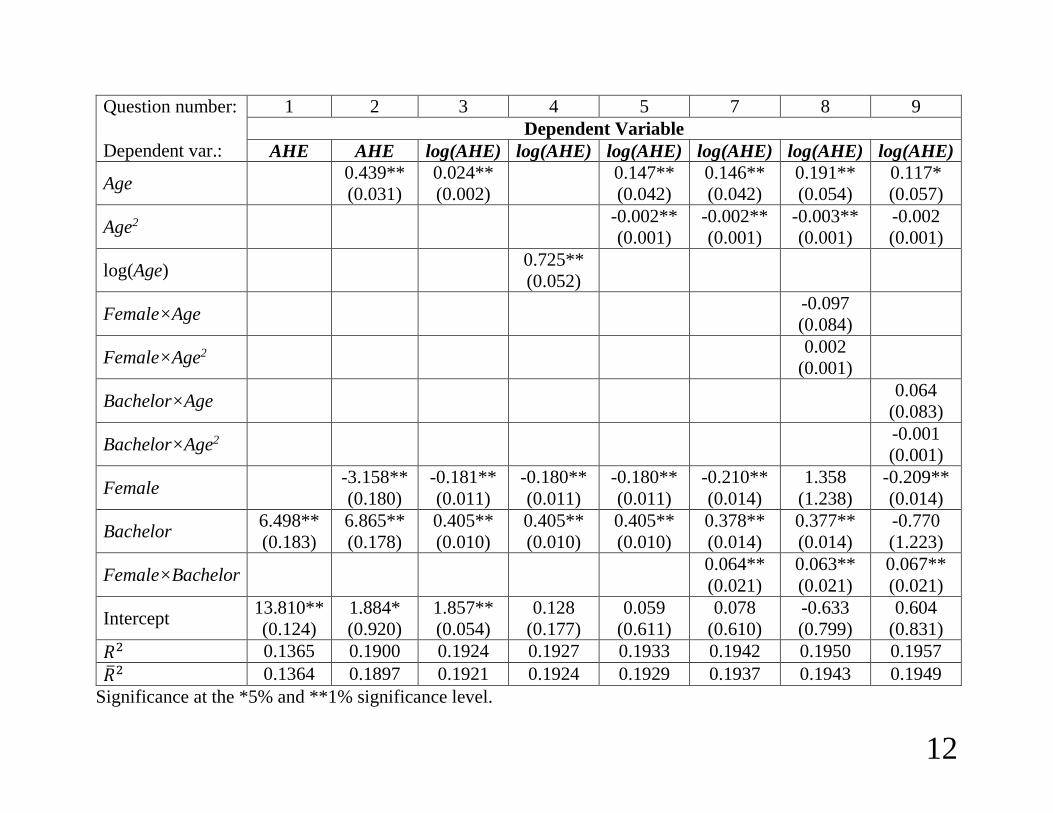
Question number: 1 2 3 4 5 7 8 9

Dependent Variable

Dependent var.: AHE AHE log(AHE) log(AHE) log(AHE) log(AHE) log(AHE) log(AHE)

Age

0.439**

(0.031)

0.024**

(0.002)

0.147**

(0.042)

0.146**

(0.042)

0.191**

(0.054)

0.117*

(0.057)

Age2

-0.002**

(0.001)

-0.002**

(0.001)

-0.003**

(0.001)

-0.002

(0.001)

log(Age)

0.725**

(0.052)

Female×Age

-0.097

(0.084)

Female×Age2

0.002

(0.001)

Bachelor×Age

0.064

(0.083)

Bachelor×Age2

-0.001

(0.001)

Female

-3.158**

(0.180)

-0.181**

(0.011)

-0.180**

(0.011)

-0.180**

(0.011)

-0.210**

(0.014)

1.358

(1.238)

-0.209**

(0.014)

Bachelor 6.498**

(0.183)

6.865**

(0.178)

0.405**

(0.010)

0.405**

(0.010)

0.405**

(0.010)

0.378**

(0.014)

0.377**

(0.014)

-0.770

(1.223)

Female×Bachelor

0.064**

(0.021)

0.063**

(0.021)

0.067**

(0.021)

Intercept 13.810**

(0.124)

1.884*

(0.920)

1.857**

(0.054)

0.128

(0.177)

0.059

(0.611)

0.078

(0.610)

-0.633

(0.799)

0.604

(0.831)

𝑅2 0.1365 0.1900 0.1924 0.1927 0.1933 0.1942 0.1950 0.1957

�̅�2 0.1364 0.1897 0.1921 0.1924 0.1929 0.1937 0.1943 0.1949

Significance at the *5% and **1% significance level.

13

a) If age increases from 25 to 26, how are earnings expected to

change?

This is a log-lin model. The interpretation of the estimated

coefficient of 0.024 on the age variable is that for a 1 unit

increase in age, earnings are expected to increase by 2.4%

b) If age increases from 50 to 51, how are earnings expected to

change?

The answer is the same as in part (a).

14

4. Run a regression of the logarithm average hourly earnings,

log(ahe), on log(age), female, and bachelor.

Results are reported in the table.

a) What is the estimated effect of age on ahe in this regression?

This is a log-log model. The coefficient of 0.725 is interpreted as

follows. For a 1% change in age, ahe is expected to increase by

0.725%.

b) If age increases from 25 to 26, how are earnings expected to

change?

This is a 4% increase in age, so ahe would increase by

approximately 0.725×4 = 2.90%

15

c) If age increases from 50 to 51, how are earnings expected to

change?

This is a 2% increase in Age, so Earnings would increase by

approximately 0.725×2 = 1.45%

16

5. Run a regression of the logarithm average hourly earnings,

log(ahe), on age, age2, female, and bachelor.

You need to use the commands:

age2 <- age^2

summary(lm(log(ahe) ~ age + age2 + female + bachelor))

17

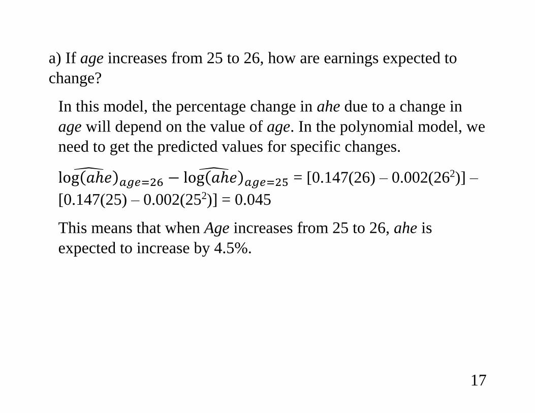
a) If age increases from 25 to 26, how are earnings expected to

change?

In this model, the percentage change in ahe due to a change in

age will depend on the value of age. In the polynomial model, we

need to get the predicted values for specific changes.

log(𝑎ℎ𝑒)̂𝑎𝑔𝑒=26 − log(𝑎ℎ𝑒)̂

𝑎𝑔𝑒=25 = [0.147(26) – 0.002(262)] –

[0.147(25) – 0.002(252)] = 0.045

This means that when Age increases from 25 to 26, ahe is

expected to increase by 4.5%.

18

b) If age increases from 50 to 51, how are earnings expected to

change?

Similar to above:

log(𝑎ℎ𝑒)̂𝑎𝑔𝑒=51 − log(𝑎ℎ𝑒)̂

𝑎𝑔𝑒=50 = [0.147(51) – 0.002(512)] –

[0.147(50) – 0.002(502)] = -0.055

This means that when age increases from 50 to 51, ahe is

expected to decrease by 5.5%. Does this make sense?

19

6. The models in questions 3, 4, and 5, are all trying to capture a

non-linear effect of age on ahe. Which model do you think is best,

and why?

We can’t use t-tests or F-tests to choose between the three

models. We could use adjusted R-squared. Based on the adjusted

R2, the model from question 5 seems to be best. However, as we

saw in question 5 it is a bit difficult to interpret the effect of age

on ahe, so for the sake of simplicity, we might choose the model

from question 4 instead.

20

7. Run a regression of log(ahe), on age, age2, female, bachelor and

the interaction term female × bachelor.

We need to create the interaction term:

fem_bach <- female*bachelor

and then include it in the model:

summary(lm(log(ahe) ~ age + age2 + female + bachelor + fem_bach))

a) What is the estimated effect of an education on earnings, for

men and for women?

Male workers with a bachelor’s degree have 37.8% higher ahe on

average than male workers without a bachelor’s degree. Female

workers with a bachelor’s degree have (37.8% + 6.4%) 44.2%

higher ahe than female workers without a bachelor’s degree.

21

b) What does the coefficient on the interaction term measure?

The 0.064 is the extra effect of an education on earnings, for

women. 6.4% more (approximately).

22

c) Do women earn less than men? Does education have a

different effect on earnings for women, then it does for men?

Use appropriate F-tests.

Do women earn less than men? The null hypothesis is that the

earnings of women are the same as the earnings of men. The

alternative hypothesis is that earnings is different between the

two groups. The model under the alternative hypothesis is the

model from the beginning of this question:

𝐻𝐴 : log(𝑎ℎ𝑒)

= 𝛽0 + 𝛽1𝑎𝑔𝑒 + 𝛽2𝑎𝑔𝑒2 + 𝛽3𝑓𝑒𝑚𝑎𝑙𝑒 + 𝛽4𝑏𝑎𝑐ℎ𝑒𝑙𝑜𝑟

+ 𝛽5(𝑓𝑒𝑚 × 𝑏𝑎𝑐ℎ) + 𝑢

This model allows for a difference between men and women.

Under the null hypothesis, there is no difference, so that the

model should be:

23

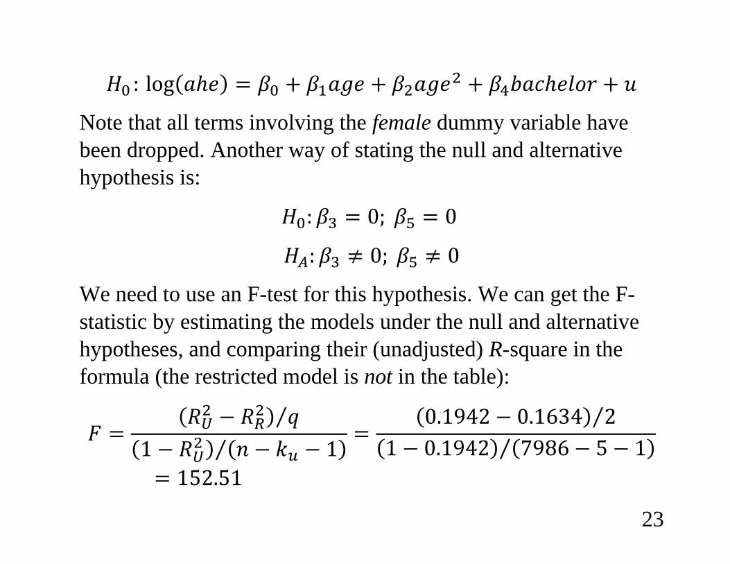
𝐻0 : log(𝑎ℎ𝑒) = 𝛽0 + 𝛽1𝑎𝑔𝑒 + 𝛽2𝑎𝑔𝑒2 + 𝛽4𝑏𝑎𝑐ℎ𝑒𝑙𝑜𝑟 + 𝑢

Note that all terms involving the female dummy variable have

been dropped. Another way of stating the null and alternative

hypothesis is:

𝐻0: 𝛽3 = 0; 𝛽5 = 0

𝐻𝐴: 𝛽3 ≠ 0; 𝛽5 ≠ 0

We need to use an F-test for this hypothesis. We can get the F-

statistic by estimating the models under the null and alternative

hypotheses, and comparing their (unadjusted) R-square in the

formula (the restricted model is not in the table):

𝐹 =(𝑅𝑈

2 − 𝑅𝑅2) 𝑞⁄

(1 − 𝑅𝑈2 ) (𝑛 − 𝑘𝑢 − 1)⁄

=(0.1942 − 0.1634) 2⁄

(1 − 0.1942) (7986 − 5 − 1)⁄

= 152.51

24

The 5% critical value for q = 2 is 3.00. We reject the null that

there is no difference in earnings between men and women.

Does education have a different effect on earnings for women,

then it does for men? The null and alternative hypotheses are:

𝐻0: 𝛽5 = 0

𝐻𝐴: 𝛽5 ≠ 0

We can use a t-test. From the table we see that the estimated

coefficient of 0.064 is significant at the 5% level, so we reject the

null hypothesis. We estimate that the effect of education on

earnings is different for men then it is for women.

25

8. Is the effect of age on earnings different for males than

females? Specify and estimate a regression that you can use to

answer this question..

We need two new interaction terms:

fem_age = female*age

fem_age2 = female*age2

and to estimate the equation:

summary(lm(log(ahe) ~ age + age2 + fem_age + fem_age2 + female + bachelor + fem_bach))

This allows for a different effect of age on ahe for men and for

women. The R2 from this regression is 0.195. Comparing this to

the R2 from the model in question 7 (0.1942) we get an F-statistic

of 3.96, suggesting we should reject the null hypothesis that the

effect of age is the same for both men and women.

26

9. Is the effect of age on earnings different for high school

graduates than college graduates? Specify and estimate a

regression that you can use to answer this question.

Similar to above. We add the new interaction terms. The F-statistic

between this new model and the one from question 7 is 7.15,

suggesting that age has a different effect depending on whether the

individual has a bachelor’s degree.