An efficient fluctuating charge model for transition metal complexes

An Efficient Fluctuating Charge Model for Transition MetalComplexes

Peter Comba,* Bodo Martin, and Avik Sanyal

A fluctuating charge model for transition metal complexes,

based on the Hirshfeld partitioning scheme, spectroscopic

energy data from the NIST Atomic Spectroscopy Database and

the electronegativity equalization approach, has been devel-

oped and parameterized for organic ligands and their high-

and low-spin FeII and FeIII, low-spin CoIII and CuII complexes,

using atom types defined in the Momec force field. Based on

large training sets comprising a variety of transition metal

complexes, a general parameter set has been developed and

independently validated which allows the efficient computa-

tion of geometry-dependent charge distributions in the field

of transition metal coordination compounds. VC 2013 Wiley

Periodicals, Inc.

DOI: 10.1002/jcc.23297

Introduction

Although partial atomic charges are not physical observables,

and therefore, are not real, they are an important concept in

chemistry and specifically in molecular mechanics. They are

fundamental for the accurate description of molecules when

electrostatic effects are not implicitly included in other force

field terms. The electrostatic interaction comprises a significant

part of nonbonded interactions between polar species (atoms

or atom groups). Traditionally, molecular mechanics force fields

assign fixed charges to specific sites within a molecule and

allow them to interact via Coulomb interactions.[1–8] These

fixed charges suffer from the disadvantage that they cannot

readjust to changes in the molecular structure or chemical

environment, for example, in geometry optimizations or mo-

lecular dynamics simulations. In some cases, the inclusion of a

dielectric constant as a damping factor in the electrostatic

equation can improve results, but for a generally applicable

force field this must remain a limited approach.

To improve on computed atomic charges, geometry-depend-

ent fluctuating charge schemes were developed based on the

electronegativity equalization principle,[9] which states that

when atoms with an infinite separation come together to form

a molecule, there is rearrangement of electronic charges, and

this continues until the electronegativities of the constituent

atoms become equal. Based on this idea, a charge model was

constructed[10] and two decades later it was the Partial Equaliza-

tion of Orbital Electronegativity (PEOE) method[11] that intro-

duced geometry-dependent charges in molecular mechanics.

PEOE-calculated charges were found to yield good results for

such charge-sensitive properties as core electron binding ener-

gies (ESCA shifts), NMR resonance shifts,[11,12] and gas-phase

proton affinities of amines.[13] Other notable examples of fluctu-

ating charge models are the electronegativity equalization

method (EEM),[14] the charge equilibration method (QEq),[15] the

atom-bond electronegativity equalization method,[16] and

charge-density based equalization schemes.[17,18]

The EE and QEq methods have found wide acceptance in

the area of organic and biomolecular force fields due to the

simplicity of the equations involved and also due to their rig-

orous theoretical basis in conceptual density functional theory

(DFT).[19–21] EEM[14] allows the direct calculation of partial

atomic charges (Qi) and molecular electronegativity veq by

using eq. (1)

veq 5 v�i 12h�i Qi1

Xj>i

Qj

rij(1)

where vi* and gi

* are the “effective” electronegativity and hard-

ness of atom i. The summation in eq. (1) represents the energy

due to interatomic interactions in the molecule. In the litera-

ture, values of vi* and gi

* for several elements can be found,

and these are calibrated against different quantum chemical

charge schemes and levels of theory.[22–25]

In the QEq method,[15] the charge distribution is calculated

by an analogous eq. (2):

veq 5 v0i 1 J0

ii Qi1

Xj>i

QjJij (2)

where vi0 and Jii

0 are the electronegativity and idempotential,

respectively, of atom i and the interatomic interaction term Jij

is calculated as a two-center Coulomb integral. Atomic ioniza-

tion energies and electron affinities (corrected for inclusion of

P. Comba, B. Martin and A. Sanyal

Anorganisch-Chemisches Institut, Universit€at Heidelberg, INF 270, D-69120,

Heidelberg, Germany

Fax: (149) 6226 546617

E-mail: [email protected]

Contract grant sponsor: German Science Foundation (DFG).

Contract grant sponsor: Heidelberg Graduate School of Mathematical and

Computational Methods for the Sciences (HGS MathComp).

VC 2013 Wiley Periodicals, Inc.

Journal of Computational Chemistry 2013, 00, 000–000 1

FULL PAPERWWW.C-CHEM.ORG

an atom in a molecule) provide a measure of vi0 and Jii

0; Jij’s

are calculated from orbital exponents of Slater-type orbitals.

The orbital exponents are taken to be charge independent

except for hydrogen, which necessitates an iterative approach

for the QEq scheme.

In transition metal chemistry, the central metal ion is usually

positively charged which makes it difficult to apply conven-

tional EEM or QEq in the majority of cases. In the QEq scheme,

the correction to ionization energies and electron affinities

due to inclusion of an atom in a molecule requires either

extensive quantum chemical calculation of the electron corre-

lation or a thorough optimization of the model parameters.

Also, the iterative nature of the method makes it computation-

ally demanding. EEM is simpler and noniterative, yet it suffers

from the drawback of using an unscreened Coulomb potential

to model the interatomic interaction term. This gives rise to

incorrect behavior of the total electrostatic energy function at

short distances. Modifications have been proposed to rectify

these deficiencies but the scope of the extensions have been

limited to organic and biomolecules, and some special zeolites

and catalysts.[26,27]

Here, we present a parameterized fluctuating charge model

that is fast, devoid of the problems of EEM, QEq and related

schemes and can be used with comparable accuracy for main

group compounds as well as transition metal complexes. Our

model contains two optimizable parameters per atom type

and is implemented in the framework of the molecular

mechanics program Momec[28–32] developed in our group.

Theory

The NIST Atomic Spectroscopy Database[33] contains data on

spectroscopic energy levels of isolated atoms and ions dis-

played in order of energy relative to the electronic ground

state. A relative energy (Erel) vs. ionization state/charge (Q) plot

can be constructed for elements from the NIST database. The

“zero” on the x-axis corresponds to a neutral atom (Q 5 0),

“11” to a singly ionized species (Q 5 11), and so on. The rela-

tive energy plotted on the y-axis is calculated by taking the

ground state (with a specific term symbol SLJ) of a particular

charged species to be of “zero” energy and using the valence

state ionization energy (VSIE) of that species as the value of

Erel, for example, when Q 5 0, the VSIE of the ground state is

taken as the value of Erel, when Q 5 11, the sum of the first

and second VSIE is taken as Erel, and so on. Using term ener-

gies to arrive at the relative energy values is essential to distin-

guish between the many possible spin states of transition

metal ions. Such fits are constructed from NIST data for the

elements carbon, nitrogen, oxygen, sulfur, chlorine, phospho-

rus, and hydrogen, and for the transition metals iron in both

low- and high-spin states, cobalt and copper (cf. Supporting

Information). It was found that in the case of all the above

elements the relative energy can be approximately expressed

as a quadratic function of the ionization state/charge as in

eq. (3).

Eat Qð Þ5Eat 0ð Þ1Aat Q1Bat Q2 (3)

In the above equation, the superscript “at” denotes isolated

atom properties, and A and B are two energy level dependent

fit parameters.

The quadratic relationship between atomic energy and ioni-

zation state has been suggested before[34] while defining the

electronegativity v of an atomic species with charge Qi as the

slope of its total electronic energy vs. ionization state curve at

Q 5 Qi, as shown in eq. (4).

v Qið Þ5oE

oQ

� �Qi

(4)

It is reasonable to assume that a similar quadratic relation-

ship exists between Erel and Q when we consider atoms in

molecules instead of isolated atoms, as shown in eq. (5).

Emol Qð Þ5Emol 0ð Þ1Amol Q1Bmol Q2 (5)

where the superscript “mol” denotes atom in molecule proper-

ties. When forming a molecule, the shape and size of the

atomic charge cloud is modified and it is expected that a sub-

sequent change in the energy-level parameters A and B

occurs. To account for this modification, it is assumed that a

simple linear relationship exists between the two sets of pa-

rameters [eqs. (6) and (7)].

Amol 5 Aat 1 DA (6)

Bmol 5 Bat 1 DB (7)

where DA and DB are corrections to the respective isolated

atom values due to incorporation in a molecule. Taking first

and second derivatives of eq. (3) with respect to charge leads

to eqs. (8) and (9).

dEmol Qð ÞdQ

5Amol 12Bmol Q (8)

d2Emol Qð ÞdQ2

52Bmol (9)

In a molecule, the interactions between constituent atoms

give rise to an additional electrostatic term in the total energy

expression. Thus, for an N-atomic molecule, the total electro-

static energy can be expressed as a function of partial atomic

charges as in eq. (10).[15,34]

E Q1::QNð Þ5XN

i51

E 0ð Þmoli 1

oEmol

oQ2

� �Qi

Qi11

2

o2Emol

oQ2

� �Qi

Q2i

!

1

XN

i51

Xj>i

QiQjDij (10)

Equation (10) consists of two parts—the first is the elec-

tronic energy of the individual atoms constituting the mole-

cule and the second is the interatomic interaction or external

FULL PAPER WWW.C-CHEM.ORG

2 Journal of Computational Chemistry 2013, 00, 000–000 WWW.CHEMISTRYVIEWS.COM

potential. The interatomic interaction term Dij is defined as the

electrostatic interaction between two unit charges separated

by a distance rij.

Use of eqs. (8) and (9) in eq. (10) yields eq. (11):

E Qi::QNð Þ5XN

i51

E 0ð Þmoli 1 Amol

i Qi13Bmoli Q2

i

� �

11

2

XN

i51

Xj 6¼i

QjDij (11)

Taking the first derivative of eq. (11) with respect to the par-

tial charges Qi gives vi, the Iczkowski–Margrave electronegativ-

ity of atom i in a molecule, as shown in eq. (12).

vi5Amoli 16Bmol

i Qi11

2

Xj 6¼i

QjDij (12)

An equation such as eq. (12) can be set up for each of the

atoms constituting the molecule, thereby yielding N simultane-

ous equations. Sanderson’s electronegativity equalization

principle[9] can now be applied to simulate a flow of charges

from high density to low and subsequent equalization of the

individual atomic electronegativities to a molecular value veq,

as given in eq. (13).

v15v25:::5vN5veq (13)

The conservation of the total charge in the molecule adds

another equation to this set. The (N 1 1) simultaneous equa-

tions can be solved for the (N 1 1) unknowns (N Qi and veq)

by standard linear algebraic methods. In matrix form, this

equation can be expressed as eq. (14).

6Bmol1

1

2D12 :::

1

2D1N 21

1

2D21 6Bmol

2 :::1

2D2N 21

: : ::: : :1

2DN1

1

2DN2 ::: 6Bmol

N 21

1 1 ::: 1 0

0BBBBBBB@

1CCCCCCCA

Q1

Q2

:::QN

veq

0BBBB@

1CCCCA5

2Amol1

2Amol2

:::2Amol

N

Qtot

0BBBB@

1CCCCA (14)

where Qtot is the total charge of the molecule.

The interatomic interaction term Dij deserves some consider-

ation. If atoms are assumed to be point charges, then the

potential due to two interacting atoms can be expressed

according to Coulomb’s inverse square law. This is a reasona-

ble approximation when electrostatic interactions between

nonbonded atoms at medium to large separation are consid-

ered, but when dealing with atoms that are bonded or in each

other’s van der Waals region, the effect due to overlap of dif-

fuse charge clouds (screening) must be taken into account.

There are two more or less obvious constraints that have to

be considered when modeling the interaction between atomic

charge clouds: (1) at large interatomic distances the functional

should behave like Coulomb’s inverse square law and (2) as

the separation approaches zero, Dij should attain a finite value.

A simple screened Coulomb-type equation that satisfies the

above constraints is eq. (15).

Dij51ffiffiffiffiffiffiffiffiffiffiffiffiffi

r2ij 1g2

ij

q (15)

where cij is a measure of the amount of screening for atom

pair ij.

Similar expressions for interatomic interaction in a mole-

cule have been proposed previously.[35,36] These methods

are aimed at rapid calculation of two-center Coulomb inte-

grals in the framework of semiempirical electronic structure

theory.

It is interesting to note that as rij tends to zero, eq. (15)

simplifies to eq. (16).

Dij rij ! 0� �

51

gij

(16)

A distance of zero between atoms i and j corresponds to an

unphysical situation, where atom i is placed on top of atom j.

This is comparable to the interaction of two electrons con-

tained in the same valence orbital of an atom. The repulsive

energy in that case is called the self-repulsion integral in semi-

empirical electronic structure theory. It has been argued that

the second derivative of atomic energy with respect to charge

can be approximately equated to this self-repulsion inte-

gral.[20],[37–39] This is shown in eq. (17).

d2E

dQ2

� �Qi

� Dij rij ! 0� �

51

gi

(17)

Comparing eq. (9) with eq. (17) gives eq. (18).

gi51

2Bmoli

(18)

Equation (15) can now be expressed in the form of eq. (19).

Dij51ffiffiffiffiffiffiffiffiffiffiffiffiffiffiffiffiffiffiffiffiffi

r2ij 1

12Bij

� �2r (19)

The atom-pair-based parameter Bij can be simplified to an

atom-type-based parameter by assuming a simple geometric

mean combining rule, as shown in eq. (20).

Bij5ffiffiffiffiffiffiffiffiBiBj

p(20)

Equation (19) is used as the expression for Dij in our fluctu-

ating charge model.



Computational Details

We have shown above that one can calculate geometry-de-

pendent partial atomic charges from a knowledge of the mo-

lecular geometry (rij), the total formal charge of the molecule

(Qtot), experimental spectroscopic energies (Aat and Bat), and

the energy correction due to incorporation of an atom in a

molecule (DA and DB). However, DA and DB cannot be

obtained in a straightforward way from experimental or theo-

retical data and hence are used as optimizable parameters in

our model.

Note that in the present implementation in Momec, energy

gradients due to the fluctuating charges are not included in

the structure optimization (energy minimization) procedure as

in the molecular mechanics concept used in Momec, intramo-

lecular electrostatic terms are not considered explic-

itly.[28,30,31,40–43] For intermolecular interactions (solvation,

crystal lattices), electrostatic potentials are of importance, and

one of the next steps clearly will be to include the correspond-

ing energy gradients.

Choice of reference data

Our aim was to develop a fluctuating charge model applicable

to compounds of the main group elements as well as transi-

tion metal complexes. As such, four training sets were devel-

oped, the first containing 28 small organic molecules (set 1),

the second containing 21 six-coordinate complexes of iron in

different oxidation and spin states (set 2), the third containing

28 six-coordinate complexes of low-spin CoIII (set 3), and the

fourth containing 19 complexes of four- and six-coordinate

CuII (set 4) (for a complete list cf. the Supporting Information).

The geometries of all molecules in set 1 were optimized at the

B3LYP/6–31G* level using Gaussian 09.[44] The structures of the

transition metal complexes in sets 2, 3, and 4 were taken from

the Cambridge Crystallographic Structure Database (CCSD).[45]

Force-field atom-type assignments within Momec are also pro-

vided in Supporting Information.

Choice of reference charges from Quantum Mechanical

methods

Atomic charges are not physical observables, and conse-

quently cannot be obtained directly from experiments. How-

ever, charges are accessible from quantum chemical

calculations. Several methods exist, such as the Mulliken Popu-

lation Analysis (MPA),[46] the Natural Population Analysis

(NPA),[47] the “Atoms in a Molecule” scheme (QTAIM),[48] Hirsh-

feld partitioning,[49] or electrostatic potential fitting.[50–53] Each

of these schemes partition the molecular electron density dif-

ferently to arrive at atomic contributions, but there is no

unique method that works equally well for all classes of com-

pounds and for all purposes.

Mulliken population analysis[46] is conceptually simple and

several fluctuating charge schemes have been calibrated based

on MPA as the method of choice but it suffers from two seri-

ous disadvantages. First, MPA is known to be basis-set de-

pendent which limits its utility, and second, the electron

density is partitioned equally between two neighboring atoms

irrespective of their electronegativity difference which often

leads to charges that do not conform to chemical intuition.

The NPA method[47] is fast, as it requires only matrix diago-

nalization and orthogonalization steps, and accurate. For a

large set of medicinally active compounds containing H, C, N,

O, and F, EEM-derived NPA charges were calculated and found

to be in good agreement with quantum chemical values.[24]

However, from studies on complexes of glyoxal diimine with

21 cations of the first row transition metals, it was concluded

that NPA charges are inconsistent with the electron transfer

scheme obtained from ab initio orbital analyses.[54]

QTAIM[48] is a theoretically robust method but calculation of

atomic charges using this scheme is computationally much

more demanding than the other schemes outlined here, espe-

cially when transition metal complexes are considered.

Electrostatic potential fitted charges, like those obtained by

CHELPG[50] or those used in AMBER,[51] are popular in force

fields as they are designed to reproduce the surface electro-

static potential accurately, but these methods also suffer from

certain inadequacies. The main criticism is that atoms buried

deep inside the molecule contribute less to the surface elec-

trostatic potential and are often assigned ambiguous charges

by the method. This is a serious problem when dealing with

transition metal complexes as a fair amount of the charge on

the complex remains with the embedded central metal ion

and its first coordination sphere. Also, many different sets of

atomic charges may yield the same surface electrostatic poten-

tial and hence, the set of atomic charges obtained by these

methods is often ambiguous and redundant. The RESP

model[52] uses restraints in the potential fitting process to rem-

edy some of these problems and yield better quality atomic

charges. Force fields with RESP charges have been developed

for organic and biological molecules and are known to per-

form well.[53]

Another quantum-chemical method that partitions electron

density into atomic contributions and yields atomic charges is

the Hirshfeld partitioning scheme.[49] The underlying concept

is that the electron density at each point in Cartesian space is

distributed among all constituent atoms. A weighting function

is then defined that is given by eq. (21):

wA rð Þ5 q0A rð Þ

q0mol rð Þ (21)

where q0A(r) is the electron density of the isolated atom A and

q0mol is the “promolecular” density, that is, the density of the

superposition of all isolated atom densities, keeping all atoms

in their original position. The individual electron densities of

the atoms are then computed using eq. (22):

qA rð Þ5 wA rð Þq rð Þ5 q0A rð Þ

q0mol rð Þ qmol rð Þ (22)

where qmol(r) is the original electron density of the molecule.

This method is known to be robust and to produce reactivity

indices that are in agreement with chemical intuition. A major



drawback, however, is that the definition of the promolecule is

arbitrary and, in most cases, derived from the electron density

of isolated atoms.[55,56] This makes the scheme unsuitable for

the application to charged species.

To overcome the problems inherent in the Hirshfeld parti-

tioning scheme, an iterative algorithm has been proposed.[57]

This eliminates the requirement to have a predefined promole-

cule, that is, the method itself determines the promolecule

from the knowledge of the molecular electron density. The

weighting function for the ith iteration is given by eq. (23):

wiA rð Þ5 qi21

A rð Þqi21

mol rð Þ (23)

The aim of this iterative algorithm is to find a converged so-

lution to the electron population. A salient feature of this

approach is that, unlike Hirshfeld’s original scheme, it can be

applied to charged species.

Keeping in mind all the merits and disadvantages associated

with the different quantum chemical charge calculation

schemes, the iterative Hirshfeld method was chosen to gener-

ate reference charges for our training sets. The level of theory

and basis set used for the calibration data sets are set 1:

B3LYP/6–31G*;[58] and sets 2, 3, and 4: B3LYP/TZVP.[59,60] The

HiPart program[61] was used to generate iterative Hirshfeld

charges from electron densities calculated at the above-men-

tioned level of theory by Gaussian 09. For set 1, geometry-

optimized structures at the B3LYP/6–31G* level were used for

the calculation of electron densities and subsequently the iter-

ative Hirshfeld charges. For the other sets, single-point calcula-

tions at the B3LYP/TZVP level were done on crystal structures

taken from the CCSD to obtain the electron densities, and sub-

sequently the iterative Hirshfeld charges.

Erel vs. Q fits from NIST data

VSIE data for the ionization states 0, 11, 12, 13, and 14

were obtained from the NIST Atomic Spectroscopy Data-

base[33] for a continuous quadratic fit of the Erel vs. Q data for

the elements considered here. The quadratic fit was obtained

using the least-squares procedure, as in eq. (3). The case of

hydrogen deserves special mention. The only ionization states

possible for hydrogen are 21, 0, and 11 (Erel for Q 5 21 state

is the electron affinity), and the fit for hydrogen uses only

these three values. The quadratic fit parameters for the ele-

ments considered here are presented in Table 1, and the fits

are given as Supporting Information.

Calibration of parameters

As mentioned earlier, our model contains two optimizable pa-

rameters per atom type, DA and DB. An automatic simplex

optimization algorithm developed in-house (distributed with

Momec) was used to achieve parameter optimizations. The

goal of the procedure was to determine a set of atom-type-

based parameters that when inserted into eq. (14) yields

atomic charges that differ only minimally from the correspond-

ing quantum chemical charges.

Results and Discussion

The process of optimization of parameters proved to be difficult

and laborious for all four reference sets. This may be attributed

to several factors. The presence of many local minima in the

multidimensional parameter space is a major hindrance to effi-

cient convergence. To avoid this, our optimizer carried out 100

random initial Monte Carlo steps to find the best set of starting

values for the parameters. This led to significant improvement

in the optimization process. Another point that deserves men-

tion in this context is the sensitivity of the parameters to the fit-

ness function, a factor that has been reported previously.[24,27]

The presence of many atom types, with some types having

only a limited number of data points, presented another chal-

lenge to the optimization process. Atom types are a fundamen-

tal part of a force field and they are determined on the basis of

element and bonding environment. In the case of transition

metal complexes, a large number of bonding environments are

possible for a particular element and, consequently, a large

number of atom types are generally used. The Momec force

field for transition metal complexes[28] uses 14 atom types each

for carbon and oxygen, 16 for nitrogen, and so on. The large

spread in reference charges for a single element depending on

the chemical environment necessitates the use of a number of

atom types for fluctuating charge calculations. In the course of

our investigations, it was observed that several atom types per

element were necessary for the development of an efficient

scheme (see Supporting Information for the atom types used in

this communication). Although we have adopted the ligand

field molecular mechanics approach in Momec, which allows to

model metal centers of different spin state with a single param-

eter set,[62,63] we have found that to obtain accurate charges,

we need to define various atom types for the four sets of iron

complexes (FeII and FeIII in high- and low-spin electronic

configurations).

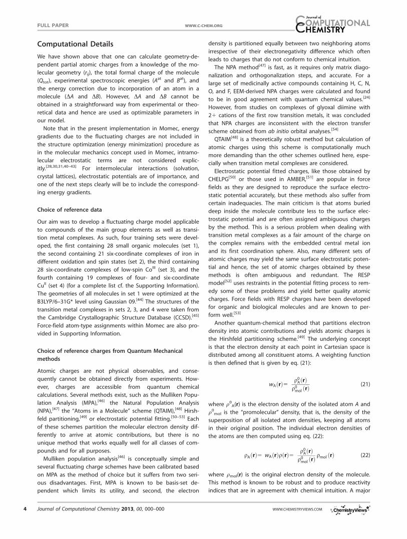
Figure 1 shows the reference (iterative Hirshfeld, calculated

at B3LYP/6–31G* level) vs. calculated (by our parameterized

model) partial atomic charges for set 1 with 28 small organic

Table 1. Quadratic fit parameters for Erel vs. Q [see eq. (3)]. Erel is plotted

in eV and Q in atomic units (au).

Element E(O)at Aat Bat

C 0.5952 20.3026 9.2837

N 1.3615 0.4519 10.2662

O 0.0353 3.1075 10.5289

S 1.3240 0.6113 7.2627

Cl 0.4786 4.3901 7.0115

P 1.7007 20.8285 7.1319

H 0.0 6.4192 7.1792

Fe (low spin) 2.5379 29.5301 8.3271

Fe (high spin) 2.8724 28.2711 8.8076

Co 2.6988 27.4608 8.8364

Cu 1.7732 25.7057 9.0887

Aat and Bat, therefore, have units of eV/au and eV/au2, respectively.



molecules. The data points are color-coded on the basis of ele-

ment. There is good correlation between the two sets of

charges (reference and calculated, r2 5 0.99) with some atom

types performing better than others in the overall optimiza-

tion. Root mean square deviations between calculated and ref-

erence charges (rmsd) and Pearson’s correlation coefficient (r2)

values for the calibrations and validation performed in this

work are given in Table 2.

A few remarks should be made concerning some features

apparent in the parameter optimization of set 1. If one consid-

ers the carbon atoms, four types are found viz., C3 (sp hybri-

dized carbon), CA (aromatic/sp2 hybridized carbon), CCO

(carboxyl/carbonyl carbon), and CT (tetrahedral, sp3 hybridized

carbon) with 2, 4, 8, and 70 data points, respectively. The CT

atom type spans a large range of reference charges (20.71

atomic units to 10.64 atomic units), and the calculated

charges are able to match this range satisfactorily. There is

only one outlier (An outlier is defined as a data point for

which the absolute difference between reference and calcu-

lated charges is larger than 10%.) for this atom type. The per-

formance of the CCO atom type (reference charge range:

10.56 to 10.97 atomic units), on the other hand, is compara-

tively poor but this may be attributed to the presence of only

eight reference data points for this type. It may be argued

that the addition of more structures containing a particular

atom type should improve the optimization results. The case

of hydrogen deserves special consideration as it has been at

the center of modifications in fluctuating charge schemes for

a long time. One approach is to use different sets of parame-

ters for hydrogen in d1 and d2 states, as suggested in the

EEM. The QEq scheme was made iterative to achieve a better

description of hydrogen charges. In another approach, only

one set of parameters for hydrogen was used to achieve satis-

factory results for a range of medicinally active compounds.[23]

It is evident from Figure 1 that a single set of parameters is

sufficient to model charges on hydrogen atoms by our model.

The best fit parameter values for this set are given in Table 3

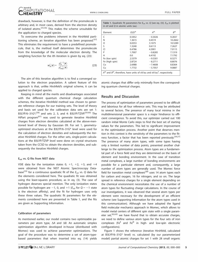
Set 2 contains 21 complexes of iron in different oxidation

and spin states, viz., high-spin FeII, low-spin FeII, high-spin FeIII,

and low-spin FeIII. Figures 2 and 3 show the reference (DFT)

vs. calculated (by our parameterized model) partial atomic

charges for the different atom types used in this set

(r2 5 0.98). It is evident from Figure 2 that the charges on the

carbon containing atom types are well reproduced by our fluc-

tuating charge model. However, the same cannot be said for

the nitrogen containing atom types. While most of the types,

Figure 1. Scatter plot of calculated vs. reference atomic charges for set 1

(small organic compounds).

Table 2. Root mean square deviation (rmsd) between calculated and ref-

erence charges and Pearson’s correlation coefficient values for the calibra-

tion and validation data sets.

Data set

Number of

data points

rmsd

(a.u.) r2

Set 1 320 0.031 0.99

Set 2 1147 0.059 0.98

Set 3 1012 0.062 0.99

Set 4 679 0.092 0.97

Combined set 3158 0.087 0.97

Validation set 799 0.096 0.95

Table 3. Optimized fluctuating charge parameters for set 1 (organic

compounds)

Atom type DA DB

C3 0.94432 27.20493

CA 21.62120 28.00252

CCO 20.54039 27.84238

CL 45.45272 36.39162

CT 1.99754 28.01017

H 25.32862 25.13978

N3 44.03830 8.34108

ND 269.25335 2.92795

NT 28.29811 23.23230

OC 20.90170 29.29922

OCO 1.74225 28.56386

OW 4.47512 27.85619

DA and DB values are given in units of eV/au and eV/au2, respectively.


(iron complexes); carbon, nitrogen, and iron atoms.



like N3 (sp hybridized nitrogen), NI (imine nitrogen), NOO

(nitrogen in a nitro group), NP (pyridine nitrogen), and NT (tet-

rahedral amine nitrogen) show good correlation, the NAH type

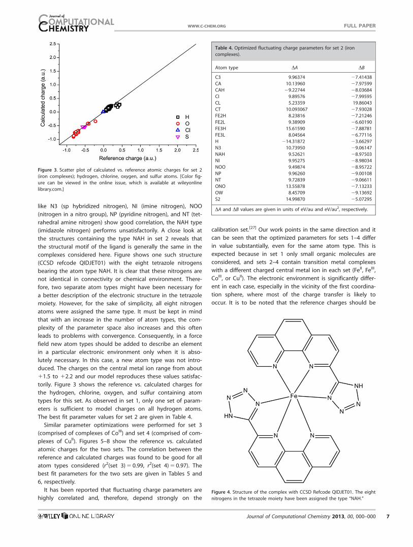
(imidazole nitrogen) performs unsatisfactorily. A close look at

the structures containing the type NAH in set 2 reveals that

the structural motif of the ligand is generally the same in the

complexes considered here. Figure shows one such structure

(CCSD refcode QIDJET01) with the eight tetrazole nitrogens

bearing the atom type NAH. It is clear that these nitrogens are

not identical in connectivity or chemical environment. There-

fore, two separate atom types might have been necessary for

a better description of the electronic structure in the tetrazole

moiety. However, for the sake of simplicity, all eight nitrogen

atoms were assigned the same type. It must be kept in mind

that with an increase in the number of atom types, the com-

plexity of the parameter space also increases and this often

leads to problems with convergence. Consequently, in a force

field new atom types should be added to describe an element

in a particular electronic environment only when it is abso-

lutely necessary. In this case, a new atom type was not intro-

duced. The charges on the central metal ion range from about

11.5 to 12.2 and our model reproduces these values satisfac-

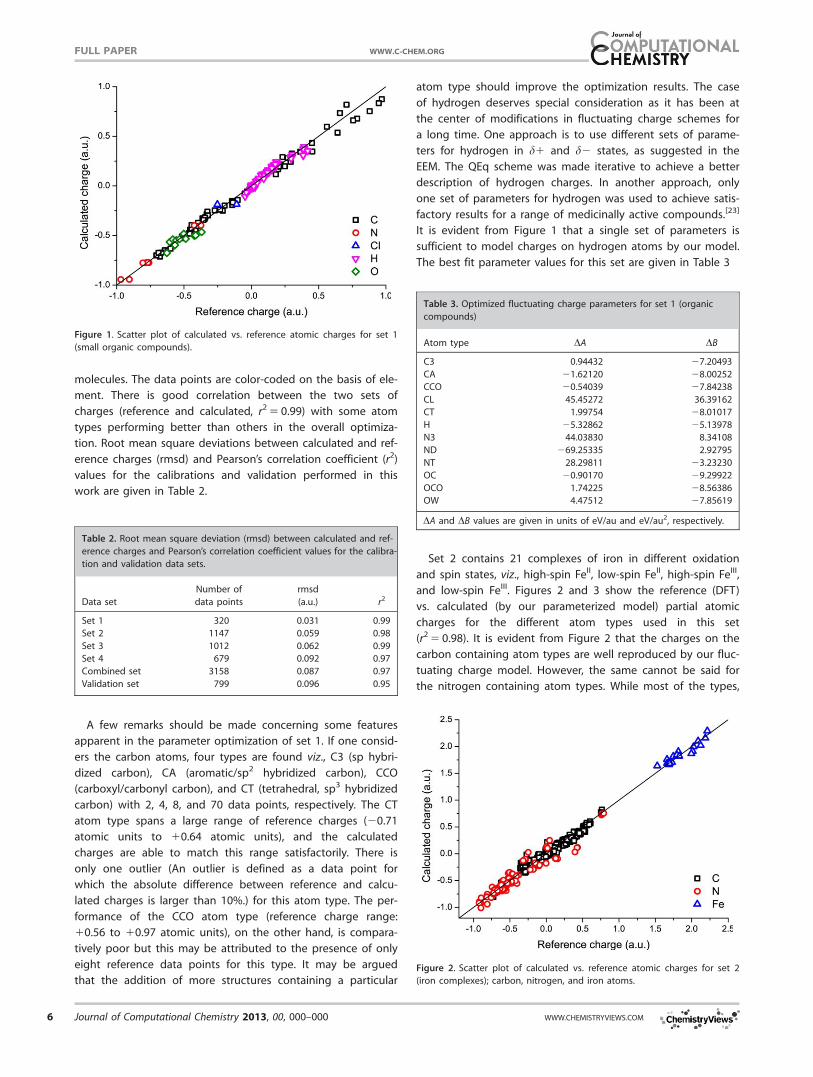
torily. Figure 3 shows the reference vs. calculated charges for

the hydrogen, chlorine, oxygen, and sulfur containing atom

types for this set. As observed in set 1, only one set of param-

eters is sufficient to model charges on all hydrogen atoms.

The best fit parameter values for set 2 are given in Table 4.

Similar parameter optimizations were performed for set 3

(comprised of complexes of CoIII) and set 4 (comprised of com-

plexes of CuII). Figures 5–8 show the reference vs. calculated

atomic charges for the two sets. The correlation between the

reference and calculated charges was found to be good for all

atom types considered (r2(set 3) 5 0.99, r2(set 4) 5 0.97). The

best fit parameters for the two sets are given in Tables 5 and

6, respectively.

It has been reported that fluctuating charge parameters are

highly correlated and, therefore, depend strongly on the

calibration set.[27] Our work points in the same direction and it

can be seen that the optimized parameters for sets 1–4 differ

in value substantially, even for the same atom type. This is

expected because in set 1 only small organic molecules are

considered, and sets 2–4 contain transition metal complexes

with a different charged central metal ion in each set (FeII, FeIII,

CoIII, or CuII). The electronic environment is significantly differ-

ent in each case, especially in the vicinity of the first coordina-

tion sphere, where most of the charge transfer is likely to

occur. It is to be noted that the reference charges should be


(iron complexes); hydrogen, chlorine, oxygen, and sulfur atoms. [Color fig-

ure can be viewed in the online issue, which is available at wileyonline

library.com.]

Table 4. Optimized fluctuating charge parameters for set 2 (iron

complexes).

Atom type DA DB

C3 9.96374 27.41438

CA 10.13960 27.97599

CAH 29.22744 28.03684

CI 9.89576 27.99595

CL 5.23359 19.86043

CT 10.093067 27.93028

FE2H 8.23816 27.21246

FE2L 9.38909 26.60190

FE3H 15.61590 27.88781

FE3L 8.04564 26.77116

H 214.31872 23.66297

N3 10.73950 29.06147

NAH 9.52621 28.97503

NI 9.95275 28.98034

NOO 9.49874 28.95722

NP 9.96260 29.00108

NT 9.72839 29.06611

ONO 13.55878 27.13233

OW 8.45709 29.13692

S2 14.99870 25.07295


Figure 4. Structure of the complex with CCSD Refcode QIDJET01. The eight

nitrogens in the tetrazole moiety have been assigned the type “NAH.”



wileyonlinelibrary.com


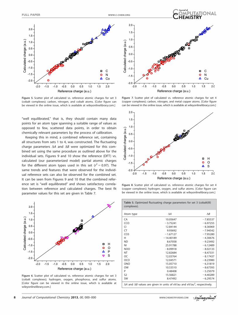
“well equilibrated,” that is, they should contain many data

points for an atom type spanning a suitable range of values as

opposed to few, scattered data points, in order to obtain

chemically relevant parameters by the process of calibration.

Keeping this in mind, a combined reference set, containing

all structures from sets 1 to 4, was constructed. The fluctuating

charge parameters DA and DB were optimized for this com-

bined set using the same procedure as outlined above for the

individual sets. Figures 9 and 10 show the reference (DFT) vs.

calculated (our parameterized model) partial atomic charges

for the different atom types used in this set (r2 5 0.97). The

same trends and features that were observed for the individ-

ual reference sets can also be observed for the combined set.

It can be seen from Figures 9 and 10 that the combined refer-

ence set is “well equilibrated” and shows satisfactory correla-

tion between reference and calculated charges. The best fit

parameter values for this set are given in Table 7.


(copper complexes); carbon, nitrogen, and metal copper atoms. [Color figure

can be viewed in the online issue, which is available at wileyonlinelibrary.com.]


(cobalt complexes); carbon, nitrogen, and cobalt atoms. [Color figure can

be viewed in the online issue, which is available at wileyonlinelibrary.com.]


(cobalt complexes); hydrogen, oxygen, phosphorus, and sulfur atoms.

[Color figure can be viewed in the online issue, which is available at

wileyonlinelibrary.com.]

Table 5. Optimized fluctuating charge parameters for set 3 (cobalt(III)

complexes).

Atom type DA DB

CA 10.05647 27.85537

CCO 23.75241 26.97255

CI 12.84144 28.36969

CT 9.93692 27.94542

CO3 21.67127 27.95280

H 214.40189 24.30676

ND 8.67058 29.23492

NI 25.91788 26.12489

NOO 28.09918 28.02133

NT 12.82684 28.47331

OC 12.03764 28.17437

OCO 12.04571 28.23980

ONO 15.05710 26.31819

OW 10.53510 28.67393

P 0.48408 25.25079

S2 15.56821 24.40289

SW 8.47492 26.29574



(copper complexes); hydrogen, oxygen, and sulfur atoms. [Color figure can

be viewed in the online issue, which is available at wileyonlinelibrary.com.]







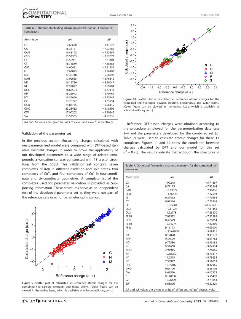
Validation of the parameter set

In the previous section, fluctuating charges calculated with

our parameterized model were compared with DFT-based iter-

ative Hirshfeld charges. In order to prove the applicability of

our developed parameters to a wide range of related com-

pounds, a validation set was constructed with 13 crystal struc-

tures from the CCSD. This validation set contains seven

complexes of iron in different oxidation and spin states, two

complexes of CoIII, and four complexes of CuII in four-coordi-

nate and six-coordinate geometries. A complete list of the

complexes used for parameter validation is provided as Sup-

porting Information. These structures serve as an independent

test of the developed parameter set as they were not part of

the reference sets used for parameter optimization.

Reference DFT-based charges were obtained according to

the procedure employed for the parameterization data sets

2–4 and the parameters developed for the combined set (cf.

Table 7) were used to calculate atomic charges for these 13

complexes. Figures 11 and 12 show the correlation between

charges calculated by DFT and our model for this set

(r2 5 0.95). The results indicate that although the structures in

Table 6. Optimized fluctuating charge parameters for set 4 (copper(II)

complexes).

Atom type DA DB

C3 2.68670 21.41673

CA 16.36161 27.93485

CAH 16.48142 27.95889

CCO 15.53365 27.82673

CI 214.50961 27.63404

CT 16.71869 27.58585

CU2 14.60021 27.51959

H 7.63825 23.962091

N3 27.46718 25.56297

NAH 17.02685 28.76346

ND 16.15726 28.96047

NI 17.57097 28.89904

NOO 218.67523 29.42131

NP 218.25943 28.70764

NT 16.35666 28.95849

OC 13.78722 29.35754

OCO 14.87735 29.06149

ONO 23.28452 25.48396

OW 17.06262 28.80845

SW 213.53535 24.92335


Figure 9. Scatter plot of calculated vs. reference atomic charges for the

combined set; carbon, nitrogen, and metal atoms. [Color figure can be

viewed in the online issue, which is available at wileyonlinelibrary.com.]


combined set; hydrogen, oxygen, chlorine, phosphorus, and sulfur atoms.



Table 7. Optimized fluctuating charge parameters for the combined ref-

erence set.

Atom type DA DB

C3 1.99248 25.71867

CA 9.71175 27.95364

CAH 28.73872 27.96836

CCO 24.66645 27.12593

CI 9.21452 27.79254

CT 9.99374 27.75363

CL 28.95984 28.82547

CO3 20.11924 27.81458

CU2 11.12778 27.85370

FE2H 7.09532 27.32388

FE2L 8.49529 26.70054

FE3H 15.54274 27.87809

FE3L 9.13113 26.65000

H 213.67888 23.69321

N3 8.17870 29.31132

NAH 9.34509 28.93783

ND 9.77580 28.99183

NI 9.59668 29.04514

NOO 2.91945 27.26065

NP 10.68059 28.73217

NT 11.0515 28.79234

OC 7.53977 29.19619

OCO 10.85102 28.42965

ONO 9.84709 28.35198

OW 8.63590 29.07575

P 0.178332 25.50470

S2 16.96424 22.71853

SW 8.68896 26.32429






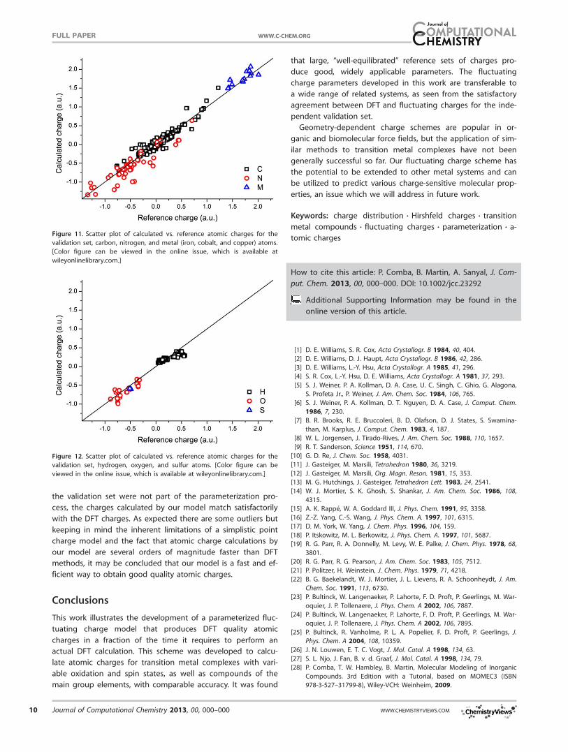
the validation set were not part of the parameterization pro-

cess, the charges calculated by our model match satisfactorily

with the DFT charges. As expected there are some outliers but

keeping in mind the inherent limitations of a simplistic point

charge model and the fact that atomic charge calculations by

our model are several orders of magnitude faster than DFT

methods, it may be concluded that our model is a fast and ef-

ficient way to obtain good quality atomic charges.

Conclusions

This work illustrates the development of a parameterized fluc-

tuating charge model that produces DFT quality atomic

charges in a fraction of the time it requires to perform an

actual DFT calculation. This scheme was developed to calcu-

late atomic charges for transition metal complexes with vari-

able oxidation and spin states, as well as compounds of the

main group elements, with comparable accuracy. It was found

that large, “well-equilibrated” reference sets of charges pro-

duce good, widely applicable parameters. The fluctuating

charge parameters developed in this work are transferable to

a wide range of related systems, as seen from the satisfactory

agreement between DFT and fluctuating charges for the inde-

pendent validation set.

Geometry-dependent charge schemes are popular in or-

ganic and biomolecular force fields, but the application of sim-

ilar methods to transition metal complexes have not been

generally successful so far. Our fluctuating charge scheme has

the potential to be extended to other metal systems and can

be utilized to predict various charge-sensitive molecular prop-

erties, an issue which we will address in future work.

Keywords: charge distribution � Hirshfeld charges � transition

metal compounds � fluctuating charges � parameterization � a-

tomic charges

How to cite this article: P. Comba, B. Martin, A. Sanyal, J. Com-

put. Chem. 2013, 00, 000–000. DOI: 10.1002/jcc.23292

Additional Supporting Information may be found in the

online version of this article.

[1] D. E. Williams, S. R. Cox, Acta Crystallogr. B 1984, 40, 404.

[2] D. E. Williams, D. J. Haupt, Acta Crystallogr. B 1986, 42, 286.

[3] D. E. Williams, L.-Y. Hsu, Acta Crystallogr. A 1985, 41, 296.

[4] S. R. Cox, L.-Y. Hsu, D. E. Williams, Acta Crystallogr. A 1981, 37, 293.

[5] S. J. Weiner, P. A. Kollman, D. A. Case, U. C. Singh, C. Ghio, G. Alagona,

S. Profeta Jr., P. Weiner, J. Am. Chem. Soc. 1984, 106, 765.

[6] S. J. Weiner, P. A. Kollman, D. T. Nguyen, D. A. Case, J. Comput. Chem.

1986, 7, 230.

[7] B. R. Brooks, R. E. Bruccoleri, B. D. Olafson, D. J. States, S. Swamina-

than, M. Karplus, J. Comput. Chem. 1983, 4, 187.

[8] W. L. Jorgensen, J. Tirado-Rives, J. Am. Chem. Soc. 1988, 110, 1657.

[9] R. T. Sanderson, Science 1951, 114, 670.

[10] G. D. Re, J. Chem. Soc. 1958, 4031.

[11] J. Gasteiger, M. Marsili, Tetrahedron 1980, 36, 3219.

[12] J. Gasteiger, M. Marsili, Org. Magn. Reson. 1981, 15, 353.

[13] M. G. Hutchings, J. Gasteiger, Tetrahedron Lett. 1983, 24, 2541.

[14] W. J. Mortier, S. K. Ghosh, S. Shankar, J. Am. Chem. Soc. 1986, 108,

4315.

[15] A. K. Rapp�e, W. A. Goddard III, J. Phys. Chem. 1991, 95, 3358.

[16] Z.-Z. Yang, C.-S. Wang, J. Phys. Chem. A. 1997, 101, 6315.

[17] D. M. York, W. Yang, J. Chem. Phys. 1996, 104, 159.

[18] P. Itskowitz, M. L. Berkowitz, J. Phys. Chem. A. 1997, 101, 5687.

[19] R. G. Parr, R. A. Donnelly, M. Levy, W. E. Palke, J. Chem. Phys. 1978, 68,

3801.

[20] R. G. Parr, R. G. Pearson, J. Am. Chem. Soc. 1983, 105, 7512.

[21] P. Politzer, H. Weinstein, J. Chem. Phys. 1979, 71, 4218.

[22] B. G. Baekelandt, W. J. Mortier, J. L. Lievens, R. A. Schoonheydt, J. Am.

Chem. Soc. 1991, 113, 6730.

[23] P. Bultinck, W. Langenaeker, P. Lahorte, F. D. Proft, P. Geerlings, M. War-

oquier, J. P. Tollenaere, J. Phys. Chem. A 2002, 106, 7887.

[24] P. Bultinck, W. Langenaeker, P. Lahorte, F. D. Proft, P. Geerlings, M. War-

oquier, J. P. Tollenaere, J. Phys. Chem. A 2002, 106, 7895.

[25] P. Bultinck, R. Vanholme, P. L. A. Popelier, F. D. Proft, P. Geerlings, J.

Phys. Chem. A 2004, 108, 10359.

[26] J. N. Louwen, E. T. C. Vogt, J. Mol. Catal. A 1998, 134, 63.

[27] S. L. Njo, J. Fan, B. v. d. Graaf, J. Mol. Catal. A 1998, 134, 79.

[28] P. Comba, T. W. Hambley, B. Martin, Molecular Modeling of Inorganic

Compounds. 3rd Edition with a Tutorial, based on MOMEC3 (ISBN

978-3-527–31799-8), Wiley-VCH: Weinheim, 2009.


validation set, hydrogen, oxygen, and sulfur atoms. [Color figure can be

viewed in the online issue, which is available at wileyonlinelibrary.com.]


validation set, carbon, nitrogen, and metal (iron, cobalt, and copper) atoms.







[29] Momec is freely available, Available at: http://www.momec.aci.uni-hei-

delberg.de. (14-01-2013)

[30] P. Comba, T. W. Hambley, M. Str€ohle, Helv. Chim. Acta. 1995, 78, 2042.

[31] J. E. Bol, C. Buning, P. Comba, J. Reedijk, M. Str€ohle, J. Comput. Chem.

1998, 19, 512.

[32] P. Comba, N. Okon, R. Remenyi, J. Comput. Chem. 1999, 20, 781.

[33] NIST Atomic Spectroscopy Database, Available at: http://www.physics.-

nist.gov/PhysRefData/ASD. (10-01-2013)

[34] R. P. Iczkowski, J. L. Margrave, J. Am. Chem. Soc. 1961, 83, 3547.

[35] K. Ohno, Theor. Chim. Acta 1964, 2, 219.

[36] G. Klopman, J. Am. Chem. Soc. 1965, 87, 3300.

[37] R. Pariser, J. Chem. Phys. 1953, 21, 568.

[38] R. Pariser, R. G. Parr, J. Chem. Phys. 1953, 21, 466.

[39] R. Pariser, R. G. Parr, J. Chem. Phys. 1953, 21, 767.

[40] P. V. Bernhardt, P. Comba, Inorg. Chem. 1992, 31, 2638.

[41] P. Comba, Coord. Chem. Rev. 1993, 123, 1.

[42] P. Comba, R. Remenyi, J. Comput. Chem. 2002, 23, 697.

[43] P. Comba, R. Remenyi, Coord. Chem. Rev. 2003, 238–239, 9.

[44] M. J. Frisch, G. W. Trucks, H. B. Schlegel, G. E. Scuseria, M. A. Robb, J.

R. Cheeseman, G. Scalmani, V. Barone, B. Mennucci, G. A. Petersson, H.

Nakatsuji, M. Caricato, X. Li, H. P. Hratchian, A. F. Izmaylov, J. Bloino, G.

Zheng, J. L. Sonnenberg, M. Hada, M. Ehara, K. Toyota, R. Fukuda, J.

Hasegawa, M. Ishida, T. Nakajima, Y. Honda, O. Kitao, H. Nakai, T.

Vreven, J. A. Montgomery Jr., J. E. Peralta, F. Ogliaro, M. Bearpark, J. J.

Heyd, E. Brothers, K. N. Kudin, V. N. Staroverov, R. Kobayashi, J. Nor-

mand, K. Raghavachari, A. Rendell, J. C. Burant, S. Iyengar, J. Tomasi,

M. Cossi, N. Rega, N. J. Millam, M. Klene, J. E. Knox, J. B. Cross, V.

Bakken, C. Adamo, J. Jaramillo, R. Gomperts, R. E. Stratmann, O.

Yazyev, A. J. Austin, R. Cammi, C. Pomelli, J. W. Ochterski, R. L. Martin,

K. Morokuma, V. G. Zakrzewski, G. A. Voth, P. Salvador, J. J. Dannen-

berg, S. Dapprich, A. D. Daniels, O. Farkas, J. B. Foresman, J. V. Ortiz, J.

Cioslowski, D. J. Fox, Gaussian 09, Revision A.02, Gaussian, Inc.: Wall-

ingford CT, 2009.

[45] F. H. Allen, Acta Cryst. 2002, B58, 380.

[46] R. S. Mulliken, J. Chem. Phys. 1955, 23, 1833.

[47] A. E. Reed, L. A. Curtiss, F. Weinhold, Chem. Rev. 1988, 88, 899.

[48] R. F. W. Bader, Atoms in Molecules—A Quantum Theory, Clarendon

Press, Oxford, 1990.

[49] F. L. Hirshfeld, Theoret. Chim. Acta 1977, 44, 129.

[50] C. M. Breneman, K. B. Wiberg, J. Comput. Chem. 1990, 11, 36.

[51] U. C. Singh, P. A. Kollman, J. Comput. Chem. 1984, 5, 129.

[52] C. I. Bayly, P. Cieplak, W. D. Cornell, P. A. Kollman, J. Phys. Chem. 1993,

97, 10269.

[53] J. Wang, P. Cieplak, P. A. Kollman, J. Comput. Chem. 2000, 21, 1049.

[54] Z. Xiong, Y. Liu, H. Sun, J. Phys. Chem. A. 2008, 112, 2469.

[55] C. F. Guerra, J.-W. Handgraaf, E. J. Baerends, F. M. Bickelhaupt, J. Com-

put. Chem. 2004, 25, 189.

[56] B. Courcot, A. J. Bridgeman, Int. J. Quantum. Chem. 2010, 110, 2155.

[57] P. Bultinck, C. V. Alsenoy, P. W. Ayers, R. Carbo-Dorca, J. Chem. Phys.

2007, 126, 144111.

[58] V. A. Rossolov, M. A. Ratner, J. A. Pople, P. C. Redfern, L. A. Curtiss, J.

Comput. Chem. 2001, 22, 976.

[59] A. Sch€afer, H. Horn, R. Ahlrichs, J. Chem. Phys. 1992, 97, 2571.

[60] A. Sch€afer, C. Huber, R. Ahlrichs, J. Chem. Phys. 1994, 100, 5829.

[61] T. Verstraelen, HiPart program, Available at: http://molmod.unigent.be/

software.

[62] C. M. Handley, R. J. Deeth, J. Chem. Theory Comput. 2012, 8, 194.

[63] A. Bentz, P. Comba, R. J. Deeth, M. Kerscher, H. Pritzkow, B. Seibold, H.

Wadepohl, Inorg. Chem. 2008, 47, 9518.

Received: 22 January 2013Revised: 18 March 2013Accepted: 22 March 2013Published online on



http://www.momec.aci.uni-heidelberg.de

http://www.momec.aci.uni-heidelberg.de

http://www.physics.nist.gov/PhysRefData/ASD

http://www.physics.nist.gov/PhysRefData/ASD

http://molmod.unigent.be/software

http://molmod.unigent.be/software

Documents

An efficient fluctuating charge model for transition metal complexes