Embed Size (px)
Citation preview
UNF Digital Commons
UNF Graduate Theses and Dissertations Student Scholarship
1999
An Efficient Implementation of the TransportationProblemAlissa Michele SustarsicUniversity of North Florida
This Master's Thesis is brought to you for free and open access by theStudent Scholarship at UNF Digital Commons. It has been accepted forinclusion in UNF Graduate Theses and Dissertations by an authorizedadministrator of UNF Digital Commons. For more information, pleasecontact Digital Projects.© 1999 All Rights Reserved
Suggested CitationSustarsic, Alissa Michele, "An Efficient Implementation of the Transportation Problem" (1999). UNF Graduate Theses andDissertations. 81.https://digitalcommons.unf.edu/etd/81
AN EFFICIENT IMPLEMENTATION OF THE TRANSPORTATION PROBLEM
by
Alissa Michele Sustarsic
A thesis submitted to the Department of Mathematics and Statistics in partial fulfillment of the requirements for the degree of
Masters in Mathematical Science
UNIVERSITY OF NORTH FLORIDA
COLLEGE OF ARTS AND SCIENCES
April,1999
Unpublished work c Alissa Michele Sustarsic

The thesis of Alissa Michele Sustarsic is approved:
Committee Chairperson
Accepted for the Department:
Chairperson
Accepted for the College:
Dean
Accepted for the University:
Dean of Graduate Studies
11
(Date)
AfWl'l 2J( ~ 'J
IJpn I. d-~ (rt;
4fd4qj
Signature Deleted
Signature Deleted
Signature Deleted
Signature Deleted
Signature Deleted
Signature Deleted

ACKNOWLEDGEMENTS
I would like to thank Dr. Adel Boules for his support, guidance, and patience he
gave throughout the time spent making this thesis possible. His encouragement and
dedication made this thesis possible. I would also like to thank Dr. Champak Panchal
and Dr. Mei-Qin Zhan for serving on the thesis committee. Thank you as well to Mrs.
Theresa Kleinpoppen who helped edit this paper.
In addition, I would like to thank my parents and family for their encouragement
throughout my time at UNF. Finally, I would like to thank my husband Jeff for his
support, patience, and encouragement which helped in ways to numerous to mention.
111
TABLE OF CONTENTS
List of Figures ...................................................................................................... v
Abstract ............................................................................................................... vi
Chapter 1
Introduction and Some Standard Results ..................................................... 1
Chapter 2
The Transportation Problem ......................................................................... 9
Chapter 3
Labeling Methods in the Primal Transportation Algorithm ...................... 29
Chapter 4
A Computer Program for the Transportation Problem ............................. 39
Chapter 5
Fortran Code for the Transportation Problem .......................................... .45
Chapter 6
Results and Conclusions ............................................................................ 69
Bibliography ....................................................................................................... 74
Vita ..................................................................................................................... 75
IV
LIST OF FIGURES
Number Page
1-1 Simplex Tableau 5
2-1 The Transportation Problem 10
2-2 Transportation Problem in the Simplex Tableau 12
2-3 Transportation Tableau 14
2-4 An Example of the Northwest Comer Rule 15
2-5 The Altered Transportation Tableau 22
3-1 An Example of a Rooted Tree 33
3-2 Example of the Indices corresponding to a Rooted Tree 34
3-3 Example of Dropping and Entering Edge ofa Tree 37
3-4 Example of a Modified Tree 38
6-1 Example of 6 x 6 Test Problem Optimal Solution 70
6-2 6 x 6 Test Problem Initial Basic Feasible Solution 71
using the NW Comer Rule
6-3 Results from the Computer Program 72
v
University of North Florida
Abstract
AN EFFICIENT IMPLEMENTATION OF THE TRANSPORTATION PROBLEM
By Alissa Michele Sustarsic
Chairperson of the Thesis Committee: Dr. Adel Boules Department of Mathematics and Statistics
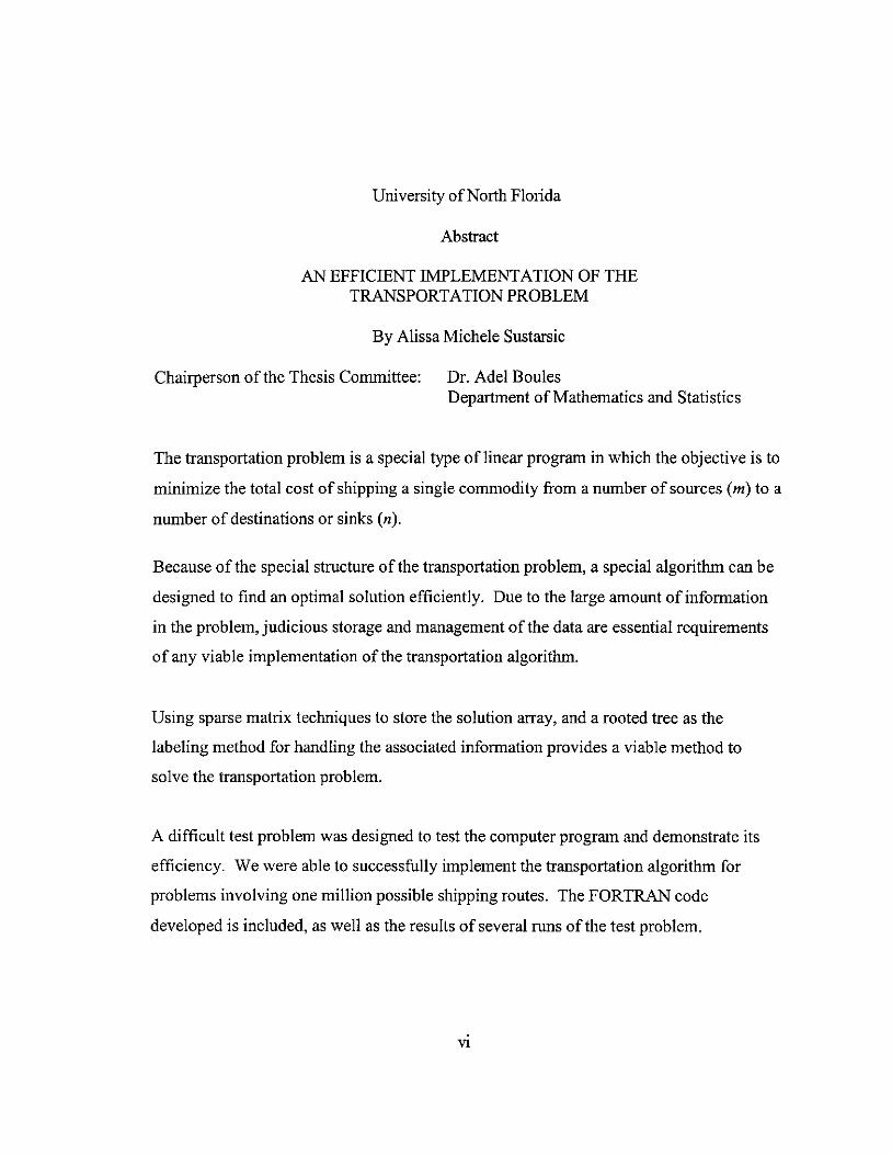
The transportation problem is a special type oflinear program in which the objective is to
minimize the total cost of shipping a single commodity from a number of sources (m) to a
number of destinations or sinks (n).
Because of the special structure of the transportation problem, a special algorithm can be
designed to find an optimal solution efficiently. Due to the large amount of information
in the problem, judicious storage and management of the data are essential requirements
of any viable implementation ofthe transportation algorithm.
Using sparse matrix techniques to store the solution array, and a rooted tree as the
labeling method for handling the associated information provides a viable method to
solve the transportation problem.
A difficult test problem was designed to test the computer program and demonstrate its
efficiency. We were able to successfully implement the transportation algorithm for
problems involving one million possible shipping routes. The FORTRAN code
developed is included, as well as the results of several runs of the test problem.
VI
Chapter 1
INTRODUCTION AND SOME STANDARD RESULTS
Linear programs are among the most widely used applications of mathematics in
industry, business, and government. The objective of linear programming is to
minimize (or maximize) a linear objective function in n real variables subject to a (finite)
set of linear constraints, which can be either equations or inequalities.
Definition: The standard form of a linear program (LP) is one of the form:
Minimize Subject to Ax=b, x~O (1.1)
where A = (aiJ) is a real m x n matrix, x and c are n-dimensional column vectors, and b
is an m-dimensional column vector.
Any linear program can be easily converted to standard form. The details of such
conversions can be found in most textbooks on linear programming. (See Taha for
details).
Definition: A point x is said to be a feasible solution of (1.1) if it satisfies the
constraints, i.e., Ax = b and x ~ O. A feasible point, xo, is said to be an optimal solution
of the linear program (1.1) if it satisfies cT Xo ::;; cT x for any feasible x. In other words,
the objective function attains its minimum value at Xo.
One can always assume that m s n and that A has full rank, i.e. rank(A) = m.
Thus A has m linearly independent columns. This can be assumed because if there are
any dependencies among the rows, there is either no solution caused by contradictory
constraints or there are redundant equations that can be eliminated.
Definition: Let B be a nonsingular m x m submatrix of A made up of m linearly
independent columns. Set all n - m components of x that are not associated with the
columns of B equal to zero. The solution to the resulting set of equations is said to be a
basic solution to Ax = b with respect to the basis B. The components ofx associated
with the columns of B are called basic variables. Because ofthe full rank assumption, a
linear program will always have basic solutions.
Definition: If a feasible solution is also basic, it is referred to as a basic feasible
solution. If it is also optimal, it is referred to as an optimal basic feasible solution.
The basic variables are not necessarily positive. If at least one of the basic variables in a
basic solution is zero, then the solution is called a degenerate basic feasible solution.
One of the most important theorems in linear programming is the Fundamental
Theorem of Linear Programming because it gives a criterion for limiting the search for
optimal solutions.
Fundamental Theorem of Linear Programming (l.a). Given the standard linear
program (1.1):
1) Ifthere is a feasible solution, there is a basic feasible solution.
2) If there is an optimal feasible solution, there is an optimal basic feasible
solution.
2
The above theorem states that the search for optimal solutions must be limited to the set
of basic feasible solutions. The proof of The Fundamental Theorem of Linear
Programming can be found in Luenberger, on page 18.
The notion of duality is central to both the development oflinear programming
algorithms and the computational aspects of the subject. Associated with every linear
programming problem there is a dual linear program, defined as follows:
Definition: The dual ofthe linear program
Minimize
is defined as
Maximize
Subject to
Subject to
Ax~b, x~O
The LP (1.2) is referred to as the primal problem and (1.3) is often called the dual
problem. A, is called the dual vector, and x is called the primal vector.
(1.2)
(1.3)
It can be shown, using the above definition, that the standard linear program (1.1)
has the following dual program:
Maximize Subject to (1.4).
The following theorem and its corollary provide the important link between the
primal and the dual problem, which will help to solve a linear program. A proof of the
Weak Duality Theorem can be found in Luenberger, on page 89.
Weak Duality Theorem (1.b). Consider the standard dual pair (1.1) and (1.4). If x and
A, are feasible for (1.1) and (1.4) respectively, then cT x ~ A,Tb .
3
This shows that a feasible vector to either problem provides a bound on the value of the
other problem. The corollary below gives a condition for the optimality of a solution.
Corollary (1.c). If Xo and ,,1,0 are feasible for (1.1) and (1.4) respectively, and if
c T Xo = A~ b, then Xo and Ao are optimal for their respective problems.
The above corollary leads to the important necessary and sufficient conditions for
optimality (See Taha, pg. 154 for the proof), called the complementary slackness
condition:
Complementary Slackness Theorem (l.d). Let x and A be feasible solutions for (1.1)
and (1.4) respectively. Then x and A are optimal for their respective problems if and only
if they meet the complementary slackness condition: (c T - ~ A)x = 0 .
One method used to solve a linear program is the simplex algorithm, which uses
the previous theorem as a stopping criterion. The simplex method proceeds from one
basic feasible solution to another where the cost, barring degeneracy, is continually
decreasing, until an optimal solution (minimum) is reached. The general philosophy
behind the primal simplex method is to generate a sequence of primal basic feasible
solutions and a corresponding sequence of vectors A (not necessarily dual feasible), such
that the complementary slackness conditions are met by each pair x and A at each
iteration. The algorithm terminates once A becomes feasible for the dual problem.
The simplex method can be performed in tableau form. The first step to the
simplex method is to put the problem in standard canonical form.
4

Definition: A standard linear program is said to be in canonical form ifit has the
following properties:
b; ~ 0 for all i, the matrix A contains the columns of the identity matrix and the cost
coefficients corresponding to the identity matrix are O.
The simplex tableau in standard canonical form is depicted in Figure (1-1).
o o
o o
0 0
0 0
a m
o
1
0
a. a J n
Y;,m+!
Ym,m+! Ymj Y mn
rm+! r. r J n
Simplex Tableau
Figure (1-1)
b
Y;o
Y mO
-zo
The r} are the reduced cost coefficients, which replace the cost coefficients once the
manipulation of the tableau starts. The columns of the identity matrix are not necessarily
the leading columns in the tableau, but the above depiction is used for the simplicity of
notation. Once a problem is in canonical form, a basic solution can be read directly from
the tableau; in the above depiction, XI through xm are the basic variables with values hI
through bm. Step two ofthe simplex algorithm consists of examining the reduced cost
5
coefficients. If all the reduced costs, rj ;::: 0, then the current basic feasible solution is
optimal. If there exists a column with a negative reduced cost coefficient and all the
entries within the column are nonpositive, there is no optimal solution. Otherwise, pick
an rj < ° and pivot aroundyho such that ~ = min{~1 Yij > 0; 1:S; i :s; m}. Return to the y Y~ Yij
beginning of step 2 until an optimal solution is determined.
The relationship between the primal and the dual problem defined above can be
seen more clearly in the simplex method when it is written in matrix notation. Let B be a
basis matrix, i.e., a square submatrix of A consisting ofthe m linearly independent
columns of A corresponding to the basic variables xB' while D consists of the columns of
A that correspond to the nonbasic variables xD• The standard linear program problem can
be rewritten, usingthepartitionA=[B,D], X=[XB,Xn], and CT=[CB~CDT], as
The basic solution, X=[XB' 0] corresponds to the basis B where x B = B-1 b because xD=O.
For any value of x D' x B = B-1 b - B-1 D x D from (1.5) and thus by substitution, the
objective function becomes
(1.6).
From (1.6), the reduced cost coefficients for the nonbasic variables xD are defined
as (1.7).
The components of r-: determine the entering variable into the basis or whether the
solution is optimal as described above.
6
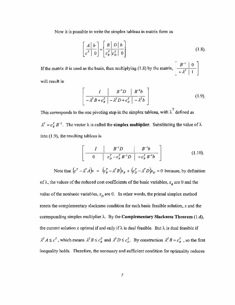
Now it is possible to write the simplex tableau in matrix form as
(1.8).
If the matrix B is used as the basis, then multiplying (1.8) by the matrix, [ B-~ I 0 ] -A 11
will result in
(1.9).
T This corresponds to the one pivoting step in the simplex tableau, with A defined as
AT = c~ B-1• The vector A is called the simplex multiplier. Substituting the value of A
into (1.9), the resulting tableau is
[ I
o (1.10).
of A, the values of the reduced cost coefficients of the basic variables, x Bare 0 and the
value of the nonbasic variables, xD are O. In other words, the primal simplex method
meets the complementary slackness condition for each basic feasible solution, x and the
corresponding simplex multiplier A. By the Complementary Slackness Theorem (l.d),
the current solution x optimal if and only if A is dual feasible. But A is dual feasible if
AT A :::;; cT , which means AT B :::;; c~ and AT D ::; c;. By construction AT B = c~ ,so the first
inequality holds. Therefore, the necessary and sufficient condition for optimality reduces
7

to c~ - AT D = C~ - C~ B-1 D ~ O. Thus, the reduced cost coefficients of the
nonbasic variables, r~ must be greater than or equal to 0 for optimality to occur.
The simplex method requires the inversion ofthe basis matrix B, and this is done
in a number of steps, or iterations, where in each step the matrix B differs from the
previous in only one column. Thus, the inversion of B can be done easily.
8
Chapter 2
THE TRANSPORTATION PROBLEM
The balanced transportation problem is a special type of linear program in
which the problem is to minimize the total cost of shipping a single commodity from a
number of sources (m) to a number of destinations or sinks (n). The simplex method can
be used to solve this problem. However, the special structure ofthe transportation
problem allows for a different technique to be created to solve these problems. This
method follows the same basic theory as the simplex method, but will be more
computationally efficient and accurate.
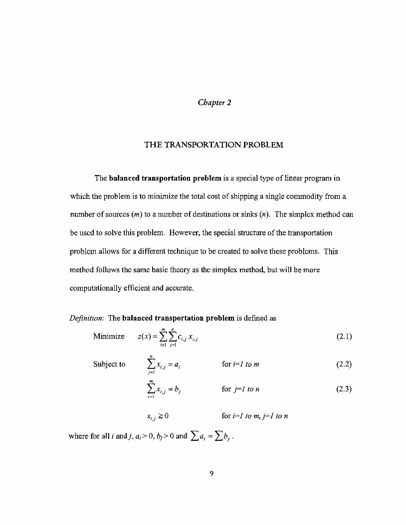
Definition: The balanced transportation problem is defined as
Minimize
Subject to
m n
z(x) = "" c .. x· . L..J L..J ',j ',j i=1 j=1
n
"x .. =a. L..J ',j , j=1
m "x .. =b. L..J ',j j i=1
for i=j to m
for j=J to n
for i=J to m,j=J to n
9
(2.1)
(2.2)
(2.3)
The only data needed for this problem is the cost of transporting the commodity per unit
from each source i to each sink} (Ci), the availability of the commodity in source i, ai,
and the demand of sink}, bj . Xijrepresents the amount shipped from source i to sink}.
m denotes the number of sources while n denotes the number of sinks. Notice that the
number of constraints of the transportation problem is m+n while the number of variables
is mn. The first set of constraints (2.2) comes from the fact that the sum ofthe shipments
from source i to all the destinations is equal to the supply available in source i. The
second set of constraints (2.3) follows similarly, by considering the sum of the shipments
from all the sources to destination}.
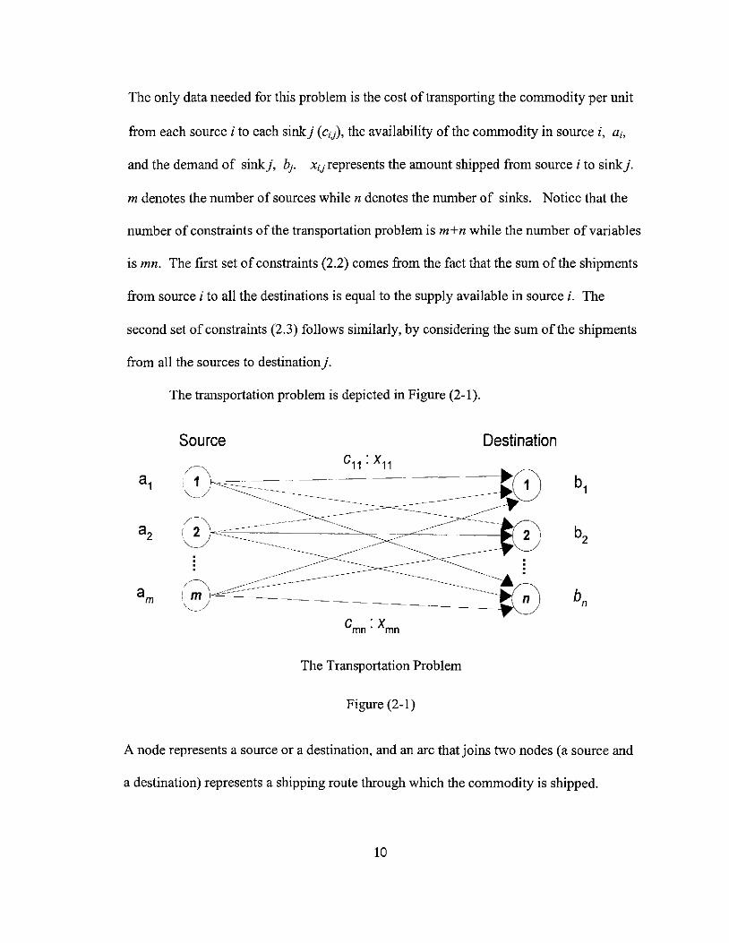
The transportation problem is depicted in Figure (2-1).
Source Destination C11 : X11
~0 a1 1 ~-~ b1 "---/ ------------------------------------------ ---------~ ----a2 2 -------------------- b2
The Transportation Problem
Figure (2-1)
A node represents a source or a destination, and an arc that joins two nodes (a source and
a destination) represents a shipping route through which the commodity is shipped.
10
The transportation problem is "balanced" because the total supply equals the total
demand, La; = Lbj . In most applications, this is not the case. However, dummy
sources or sinks can always be added to the problem to make it balanced. Being a
"balanced" problem is an important feature of the transportation model and as we will
now show is the necessary and sufficient condition for the transportation problem to be
feasible. To show the sufficiency of this condition, let S be equal to the total supply
"" a;bj (which is also equal to the total demand), S= L..Ja; = L..Jbj . Let X;,j = S for i=l, ... ,m
n n a. b. m m a. b. and}=l, ... ,n. So LX;,j = LT=a; and LX;,j = LT=bj . Therefore,xis
j=1 j=1 ;=1 ;=1
feasible, and a feasible solution always exists for the balanced transportation problem.
m n n
Conversely, ifthe transportation problem has a feasible solution x, then L L X;,j = Lbj ;=1 j=1 j=1
n m m
and LLX;,j = La;. Therefore, La; = Lbj , which establishes the necessity ofthe j=1 ;=1 ;=1
balance.
The feasible region is also bounded, since x;,j ~ a; and X;,j ~ bj for all i and}.
Thus, xij ~ min {a; , b j IV i, j} , and since the feasible region is also closed, it is actually
compact. Thus, the objective function will always achieve a minimum value (an optimal
solution).
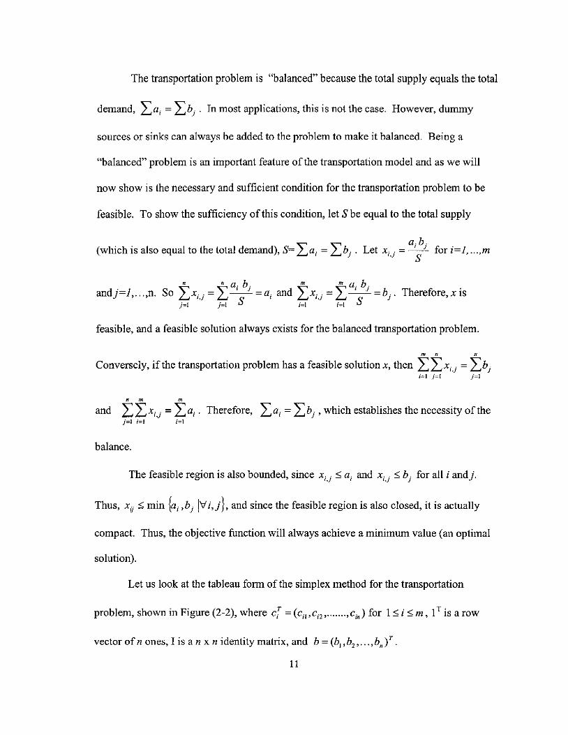
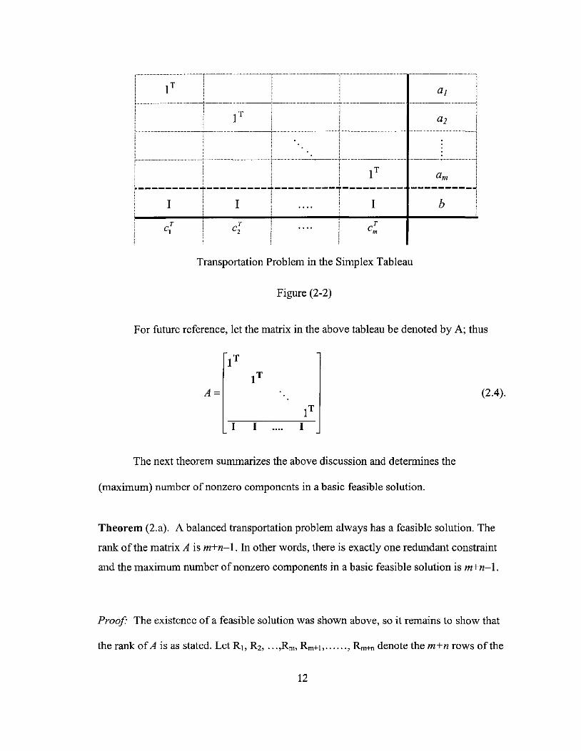
Let us look at the tableau form of the simplex method for the transportation
problem, shown in Figure (2-2), where c{ = (c;pc;z, ....... 'c;n) for 1 ~ i ~ m, 1 T is a row
vector ofn ones, I is a n x n identity matrix, and b = (bpbz, ... ,bn)T.
11
.......... ---........................................ -~-_ .......................... _._--,--........................................ _ ... _-_ ................... _ ... _ .......................................................... __ ............ -i
~-............................................ ---+--....... - ..................... -... ----_.- ........................... _ .... -.... __ .............................. _. __ .. ........... ~ .... --... -.......................... !
I T a2
-.-.--+---............................ - .. --.... L ............................ --.. - ................... -- ! • i · ........ ·1
..................... _
........ 1............. I . ,...................... .. .......................... _ .... _-...1.. ...................... _. - .. --..... ~.-.. ------ ........... --.--.. -......... - .......... · ... ·1
IT ---------~---------~---------~--------- ---------~
I I I b
Transportation Problem in the Simplex Tableau
Figure (2-2)
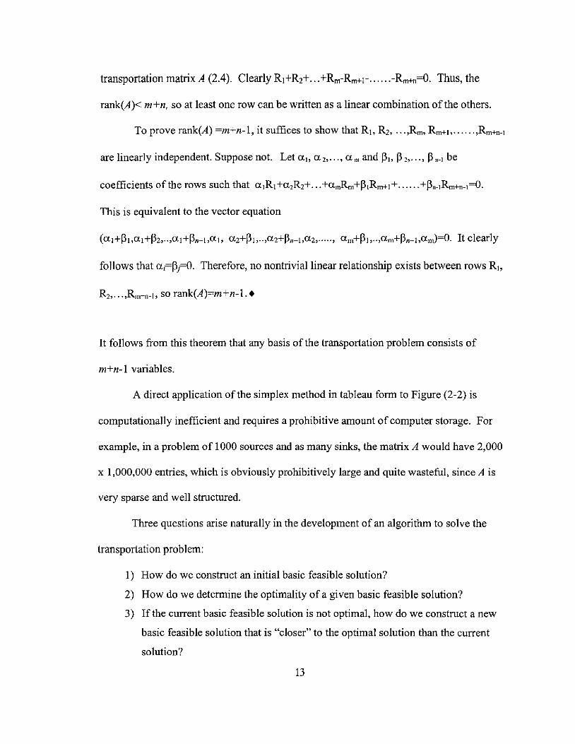
For future reference, let the matrix in the above tableau be denoted by A; thus
IT IT
A= (2.4).
IT I I I
The next theorem summarizes the above discussion and determines the
(maximum) number of nonzero components in a basic feasible solution.
Theorem (2.a). A balanced transportation problem always has a feasible solution. The
rank of the matrix A is m+n-I. In other words, there is exactly one redundant constraint
and the maximum number of nonzero components in a basic feasible solution is m+n-I.
Proof The existence of a feasible solution was shown above, so it remains to show that
the rank of A is as stated. Let Rl, R2, ... ,Rm, Rm+1, •••••• , Rm+n denote the m+n rows of the
12
transportation matrix A (2.4). Clearly RI+R2+ ... +Rm-Rm+l- ...... -Rm+n=O. Thus, the
rank(A)< m+n, so at least one row can be written as a linear combination of the others.
To prove rank(A) =m+n-1, it suffices to show that RI, R2, ... ,Rm, Rm+l, ...... ,Rm+n-t
are linearly independent. Suppose not. Let ah a 2,. .. , a m and Ph P 2,· .. , P n-t be
coefficients of the rows such that atRl+a2R2+ ... +amRm+PtRm+I+ ...... +Pn-tRm+n-t=O.
This is equivalent to the vector equation
follows that al=PrO. Therefore, no nontrivial linear relationship exists between rows Rio
R2, ... ,Rm+n-I, so rank(A)=m+n-l..
It follows from this theorem that any basis of the transportation problem consists of
m+n-1 variables.
A direct application of the simplex method in tableau form to Figure (2-2) is
computationally inefficient and requires a prohibitive amount of computer storage. For
example, in a problem of 1000 sources and as many sinks, the matrix A would have 2,000
x 1,000,000 entries, which is obviously prohibitively large and quite wasteful, since A is
very sparse and well structured.
Three questions arise naturally in the development of an algorithm to solve the
transportation problem:
1) How do we construct an initial basic feasible solution?
2) How do we determine the optimality of a given basic feasible solution?
3) If the current basic feasible solution is not optimal, how do we construct a new
basic feasible solution that is "closer" to the optimal solution than the current
solution?
13
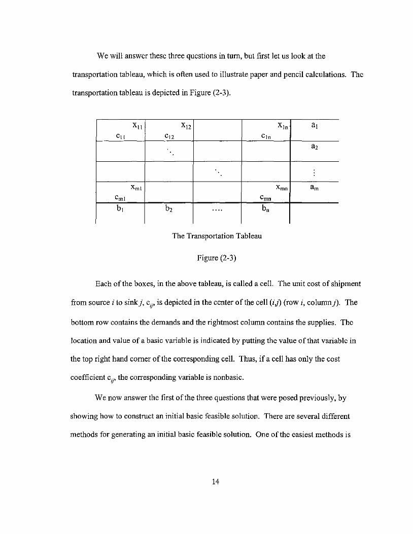
We will answer these three questions in tum, but first let us look at the
transportation tableau, which is often used to illustrate paper and pencil calculations. The
transportation tableau is depicted in Figure (2-3).
XlI X12 Xin al ClI C12 Cin
a2
XmI Xmn am CmI Cnm bi b2 .... bn
The Transportation Tableau
Figure (2-3)
Each of the boxes, in the above tableau, is called a cell. The unit cost of shipment
from source i to sink}, cij' is depicted in the center of the cell (iJ) (row i, column}). The
bottom row contains the demands and the rightmost column contains the supplies. The
location and value of a basic variable is indicated by putting the value of that variable in
the top right hand comer of the corresponding cell. Thus, if a cell has only the cost
coefficient cij' the corresponding variable is nonbasic.
We now answer the first of the three questions that were posed previously, by
showing how to construct an initial basic feasible solution. There are several different
methods for generating an initial basic feasible solution. One of the easiest methods is
14
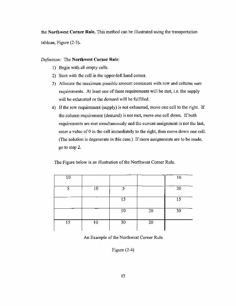
the Northwest Corner Rule. This method can be illustrated using the transportation
tableau, Figure (2-3).
Definition: The Northwest Corner Rule:
I) Begin with all empty cells.
2) Start with the cell in the upper-left hand comer.
3) Allocate the maximum possible amount consistent with row and column sum
requirements. At least one of these requirements will be met, i.e. the supply
will be exhausted or the demand will be fulfilled.
4) Ifthe row requirement (supply) is not exhausted, move one cell to the right. If
the column requirement (demand) is not met, move one cell down. Ifboth
requirements are met simultaneously and the current assignment is not the last,
enter a value of 0 in the cell immediately to the right, then move down one cell.
(The solution is degenerate in this case.) If more assignments are to be made,
go to step 2.
The Figure below is an illustration ofthe Northwest Comer Rule.
10 10
5 10 5 20
15 15
10 20 30
15 10 30 20
An Example of the Northwest Comer Rule
Figure (2-4)
15

The solution determined by the Northwest Comer Rule is clearly feasible. The
following concept is needed to establish the fact that it is basic.
Definition: A loop is an ordered sequence of at least four cells of an array if:
1) Any two consecutive cells lie in either the same row or same column.
2) No three consecutive cells lie in the same row or column.
3) The last cell in the sequence has a row or a column in common with the first
cell in the sequence.
The following theorem gives a necessary and sufficient condition for a feasible
solution of the transportation problem to be basic:
Theorem (2.b). In a balanced transportation problem, a set of m+n-l variables is basic if
and only the corresponding cells in the transportation tableau contain no loops.
Proof Assume the set of cells contains a loop. Allocate a value of + 1 and -1 alternately
among the cells in the loop, and entries of 0 in all the rest ofthe cells not in the loop.
Then the sum of all entries in the rows and columns of the array is zero. This
corresponds with the multiplication of the constraints of the transportation problems (2.1)
that coincide with a cell in the loop with + 1 and by -1 respectively. If the columns are
summed, the result will be the zero vector. Hence the set of the column vectors is linear
dependent. Hence, any set of cells that contain a 8-100p will be linearly dependent.
Therefore, the set of cells can not be a basis.
Let ~ be a set of cells corresponding to a basis and assume that ~ contains a loop.
As seen from theorem (2.a), the columns corresponding to ~ are linear independent.
Thus there does not exist a nonzero linear combination ofthe column vectors that equal
16

the zero vector. Therefore, there can not be two entries in each row. This leads to a
contradiction because a loop must contain two entries within each row that contains an
entry of the loop .•
We now tum to the question of finding a criterion for determining the optimality
of a basic feasible solution. The notion of a triangular matrix is needed in order to
achieve this. Simply put, a triangular matrix is a nonsingular square matrix that becomes
lower triangular after an appropriate permutation of its columns and rows.
Definition: A matrix is said to be a triangular matrix if it satisfies the following
properties:
1) The matrix has a row that contains exactly one nonzero entry.
2) The submatrix, formed from the matrix by crossing out the row and the column
that contains the nonzero entry, also satisfies property (1). This procedure can
be repeated until all rows and columns are crossed out.
Clearly, any matrix that satisfies the above 2 properties is a triangular matrix. Therefore,
it can be put in lower triangUlar form by arranging the rows and columns in the order that
was determined by the procedure listed above.
The importance of a matrix Mbeing triangular is that the matrix equations,
M x = d , can then be solved by backward substitution. So, if M is a triangular matrix,
then after the reordering of the columns and the rows, the system takes the form
M' x = d , where M' is lower triangular, and can be solved by backward substitution.
17
An important structural property of the transportation problem is given by the
following theorem:
Basis Triangularity Theorem (2.c). Every basis of the transportation problem is
triangular.
Proof Consider the transportation matrix A (2.4). Let us change the sign ofthe first half
of the system that corresponds to the supply constraints. Then, the coefficient matrix of
the system will have entries of + 1, 0, or -1. By theorem (2.a), one redundant equation can
be eliminated. From the resulting matrix M, form a basis B by selecting a square
nonsingular submatrix with m+n-l columns.
Each column in A contains two nonzero entries including a + 1 and -1, and,
hence, each column in B contains at most two nonzero entries also. Thus, the total
nonzero entries of B will be at most 2(m+n-l). If every column of B contained two
nonzero entries, the sum of all the rows in B would be 0 as seen from theorem (2.a). This
is a contradiction to B being nonsingular. Therefore, the nonzero entries in B must be
less than 2(m+n-l). Since B is of order (m+n-l), there must be a row with only one
nonzero entry. This verifies the first property of a triangular matrix. A similar argument
can be made for the submatrix created from deleting the row and column of B that
contained the single nonzero entry; that submatrix will also have a single row with only
one nonzero entry. This argument can be repeated, which establishes that the basis B is
triangular .•
18
The triangularity of the basis makes it unnecessary to explicitly calculate the
inverse of the basis B-1, in order to calculate the simplex multipliers, given by AT B = C~ •
Therefore, for a transportation problem, because the basis is triangular, the simplex
method at this step simplifies to solving for the simplex multipliers directly, using
backward substitution.
The next important step of the transportation problem is the form of the dual.
The dual of the transportation problem is in the form of(l.4). Let A.T=(u~ vT) be
partitioned in accordance with the natural partitioning of A. Thus uT = (UI," .,urn) and vT
= (VI" .. ,vn)· Remembering that A has two nonzero entries in each column, which can be
seen from (2.4), the components corresponding to Cij in the constraints /IT A ~ cT of the
dual can be rewritten as U i + Vj ~ cij' Summarizing, the dual ofthe transportation
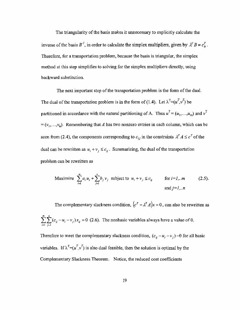
problem can be rewritten as
m n
Maximize Z>i ui + Z)j Vj subject to U i + Vj ~ cij for i=i, .. m (2.5). i=1 J=I
andj=i, .. n
The complementary slackness condition, (c T - Ar A)x = 0, can also be rewritten as
m n
LZ)cij -u i -vj)xij = 0 (2.6). The nonbasic variables always have a value ofO. i=1 j=1
Therefore to meet the complementary slackness condition, (cij -u i -v)=O for all basic
variables. If A. T=(u~ vT) is also dual feasible, then the solution is optimal by the
Complementary Slackness Theorem. Notice, the reduced cost coefficients
19
r ij = (Cij - U j - v j) , for the nonbasic cells xij. So again the criterion for optimality reduces
down to whether the reduced costs are nonnegative for the nonbasic variables.
Therefore, after an initial basic feasible solution is found for the primal, the
simplex multipliers, 'A=(u, v) need to be computed and then tested for feasibility. From
the primal simplex method, the multipliers are computed from solving AT B = c~. A
column from A (2.4), that corresponds to the basic variable xij, will contain exactly two
+ I entries, corresponding to the ith position within the top portion (sources) and to the /h
position ofthe bottom portion (sinks). Thus, each column corresponding to the basic
variable xij, will generate the simplex multiplier equation, Uj + Vj = cij. Remembering that
one constraint is redundant, one ofthe multipliers can be assigned an arbitrary value. For
simplicity, set vn=O. The set of equations Uj + Vj = Cij (for all basic variables) can now be
solved easily by backward substitution. Notice, by solving these equations, the
complementary slackness condition is met.
Therefore, testing whether the simplex multiplier is dual feasible will define the
criterion of whether the solutions are optimal. If (u,v) satisfies the inequality,
U j + Vj :::; cij for all i and}, it is dual feasible. Since this inequality is already met for all
basic cells (i,j), the inequality, cij - U j - v j ~ 0 for the nonbasic cells (i,j) is a necessary
and sufficient condition for optimality. This is equivalent to calculating the reduced cost
coefficients and if they are all nonnegative, the solution (u, v) is feasible for the dual
problem and (u, v) and x are optimal for their respective problems.
20

Therefore, the next step in the primal transportation algorithm is to calculate the
reduced costs, rli = Cij -Uj -vj . They only need to be calculated for the nonbasic cells
because by design, the reduced cost for the basic cells is O.
If the reduced cost coefficients are not all nonnegative for the basis, then a new
basis must be constructed. First, the next theorem allows us to use the reduced cost
coefficients from step to step instead of keeping the original cost coefficients.
Theorem C2.d). Let r ij represent the reduced cost coefficients. Then 2>ij xij differs j,j
from the objective function, ICij xij by a constant. Therefore, an optimal vector for j,J
I eij xij is also an optimal vector for I rij Xij . W W
= IIcij Xij - IcIxij)u j - IcIXij)Vj j j j
= IIcijxij - Iaju j - IbjVj j
•
Therefore, during the calculations to solve the transportation problem, the reduced
cost coefficients can be used to find the optimal solution. For the reason stated above,
using the reduced cost coefficients to find an optimal solution will be helpful to show the
solution meets the complementary slackness condition.
Once an initial primal feasible solution is recorded in the tableau, U and v can be
recorded in the place allocated for a and b. From the previous theorem, the reduced costs
21
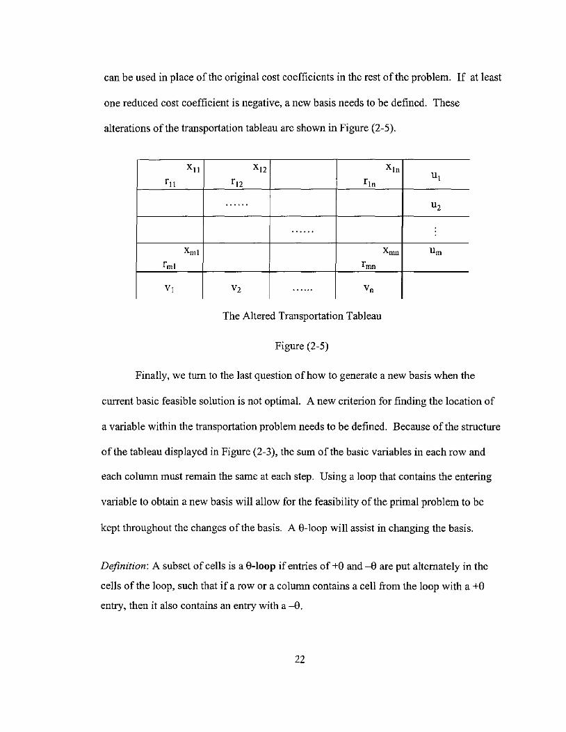
can be used in place of the original cost coefficients in the rest ofthe problem. If at least
one reduced cost coefficient is negative, a new basis needs to be defined. These
alterations of the transportation tableau are shown in Figure (2-5).
XlI x 12 x ln r ll r12 rln
u l
...... U2
. .....
Xrnl Xrnn urn frnl fmn
VI V2 ...... Vn
The Altered Transportation Tableau
Figure (2-5)
Finally, we tum to the last question of how to generate a new basis when the
current basic feasible solution is not optimal. A new criterion for finding the location of
a variable within the transportation problem needs to be defined. Because ofthe structure
of the tableau displayed in Figure (2-3), the sum ofthe basic variables in each row and
each column must remain the same at each step. Using a loop that contains the entering
variable to obtain a new basis will allow for the feasibility of the primal problem to be
kept throughout the changes of the basis. A 8-100p will assist in changing the basis.
Definition: A subset of cells is a 8-loop if entries of +8 and -8 are put alternately in the
cells of the loop, such that if a row or a column contains a cell from the loop with a +8
entry, then it also contains an entry with a-8.
22
A basis for the transportation problem has been shown to not contain a loop and
also to be triangular. A collection of cells of the transportation array is a minimal
linearly dependent set if and only if(l) it is linearly dependent and (2) no proper subset
of it is linearly dependent. By the definition ofa 8-100p, it is clear that a 8-100p is a
minimal linearly dependent set. The following theorem will define a criterion of how to
find a unique 8-100p.
8-Loop in B u {(P,q)} Theorem (2.t). Suppose B is a basic set ofm+n-l cells from the
mxn transportation array and {(P,q)} is a nonbasic cell. Then the collection of cells
B u {(P,q)} contains exactly one 8-100p and this 8-100p contains the nonbasic cell.
Proof Since B is a basic set, B is linearly independent so it can not contain a 8-100p.
Thus, ifthere is a 8-100p in B u {(P,q)} , the loop must contain {(P,q)}. Since the rank of
A (2.1) is m+n-l, no subset ofm+n cells is linear independent. So B u {(P,q)} is linearly
dependent. From the previous theorems, B u {(P,q)} contains at least one 8-100p. From
Linear Algebra, a set containing a basis and exactly one nonbasic column vector contains
a unique minimal linearly dependent set. Thus, the set of column vectors contained in the
set B U {(P,q)}, contains exactly one 8-100p .•
To find a 8-100p in B U {(P,q)} , place an entry of +8 in the nonbasic cell (p,q).
Then make alternating entries of -8 and +8 among the basic cells, such that each row and
column contains a +8 and -8 or none at all. The cells marked by +8 and -8 creates a
23
unique 8-100p. Cells marked +8 are called recipient cells and cells marked -8 are called
donor cells. 8-100ps can be used to change the basis, which is shown in the next theorem.
Theorem (2.g). Let B be a basis from A (ignoring one row) and let d be another column
corresponding to a nonbasic variable which is entering the basis. The vector y=B-1 d will
give the changes in the current basic variables when the new variable is entered. The
components ofthe vector y=B-1 dare + 1, -lor O.
Proof Let y be a solution to By=d. Then y is the linear combination of the basis that
represents d. This can be solved by Cramer's rule as Yk = det(Bk ) where Bk is the matrix det(B)
obtained by replacing the kth column of B by d. Since B is triangular, it may be put into
lower triangular form with 1 's on the diagonal by a combination ofrow and column
interchanges. Therefore det(B)= + 1 or -1. Because any square submatrix of A will only
contain entries of 0 or 1 with a maximum of two 1 's in each column by the design ofthe
matrix A, every determinant of any submatrix of A will have a value of + 1, -1, or 0, so
det(Bk)= 0, +1, or-I. ThereforeYk=O, +1, or-1.+
The significance of the above theorem is that the current basic variables will
change by + 1, -1, or 0 when a new variable is entered into the basis, at unit level. If the
new variable has a value of 8, then the current basic variables will then change by +8, -8,
or 0 corresponding to whether it is a recipient cell, donor cell, or a cell not within the
loop, respectively.
24
Therefore, to change the basis, pick a nonbasic variable (xp,q) corresponding to a
negative cost coefficient (usually the most negative) to enter the basis. Find the unique
8-100p in the set B u {(P,q)}. Place a +8 in the cell (p,q) and the entries -8 and +8
alternatively among the cells within the loop. Let x represent the current basic feasible
solution. Therefore, the values of the new basic feasible solution is XiJ = xij + 8 , xij - 8,
or xij' depending on whether (i,j) is a recipient cell, a donor cell, or a cell not within the
loop, respectively and xpq=8. All other nonbasic variables have a value of zero.
All of the values within the vector x must remain nonnegative so that the
solution remains feasible at every step. By choosing 8 by the minimum ratio rule,
8 = min { xrs ; (r,s) a donor cell}, x will always remain feasible. Therefore, 8 is
determined at each step so that the primal feasibility of x is always retained. The donor
cell from which 8 is attained, is the cell that is leaving the basis. If more than one donor
cell meets this criterion, one is arbitrarily chosen and is replaced in the basis by the cell
(p,q). Because 8 ~ 0, the objective function at each step will at most be equal to the
previous system. The objective function at each step will be z( x )+rpq8. This can be seen
by looking at the value of the objective function at two consecutive steps. At the first
step,
z(X)= LCij xij = LLrij xij + Lai ui + Lbj Vj i j
with the value ofrij equal to ° for the current basic variables and the value of xij equal to
° for the nonbasic variables. Therefore, the objective function has a value of
z(X)= Laiui + Lbjvj . i j
25
The objective function corresponding to the new basic feasible solution is
z(x)= LLrij Xij + Lai U i + Lb j Vj = rpq Xpq + Lai U i + Lb j Vj i j i j
because the only value changed from the previous objective function, that was not
multiplied by 0, is Xp,q= 8. Therefore, the objective function differs by rpqXpq where xpq=8
from the previous step.
Therefore, to summarize the transportation algorithm:
1) Compute an initial basic feasible solution.
2) Compute the simplex multipliers and the reduced cost coefficients. If all
reduced cost coefficients are nonnegative, stop; the solution is optimal.
Otherwise, go to 3.
3) Select a nonbasic variable corresponding to a negative reduced cost
coefficient to enter the basis. Find the unique 8-100p and update the solution.
Go back to 2.
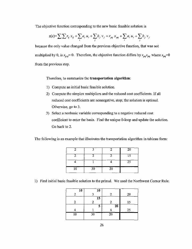
The following is an example that illustrates the transportation algorithm in tableau form:
2 3 2 20
2 2 2 15
4 1 4 25
10 30 20
1) Find initial basic feasible solution to the primal. We used the Northwest Comer Rule.
10 10 2 3 2 20
15 2 2 2 15
5 20 4 1 4 25 10 30 20
26
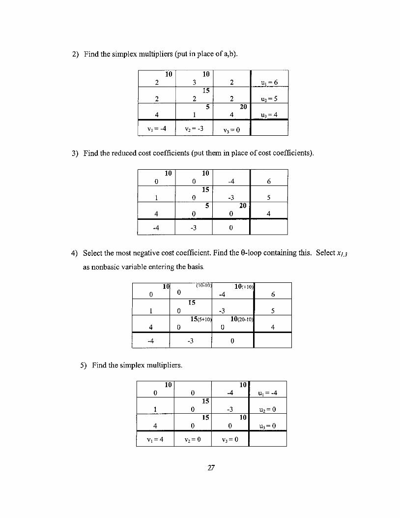
2) Find the simplex multipliers (put in place of a,b).
10 10 2 3 2 uI=6
15 2 2 2 U2= 5
5 20 4 1 4 u3=4
VI =-4 V2= -3 V3= 0
3) Find the reduced cost coefficients (put them in place of cost coefficients).
10 10 0 0 -4 6
15 1 0 -3 5
5 20 4 0 0 4
-4 -3 0
4) Select the most negative cost coefficient. Find the 8-loop containing this. Select Xu
as nonbasic variable entering the basis.
10 (10-10 10(+10 0 0 -4 6
15 1 0 -3 5
15(5+10 10(20-10 4 0 0 4
-4 -3 0
5) Find the simplex multipliers.
10 10 0 0 -4 UI =-4
15 1 0 -3 U2=O
15 10 4 0 0 U3= 0
vI=4 V2= 0 V3= 0
27
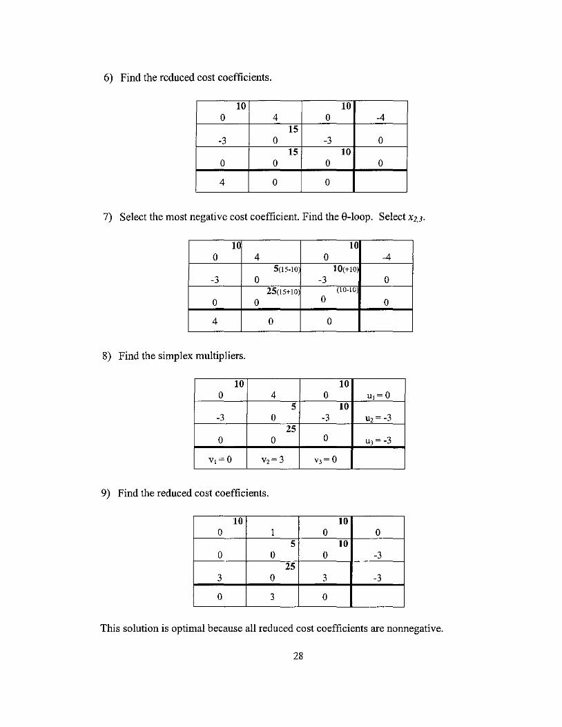
6) Find the reduced cost coefficients.
10 10 0 4 0 -4
15 -3 0 -3 0
15 10 0 0 0 0
4 0 0
7) Select the most negative cost coefficient. Find the 8-loop. Select X2,3.
10 10 0 4 0 -4
5(15-10 10(+10 -3 0 -3 0
25(15+10 (10-10
0 0 0 0
4 0 0
8) Find the simplex multipliers.
10 10 0 4 0 U1=O
5 10 -3 0 -3 U2= -3
25 0 0 0 U3= -3
V1=O V2= 3 V3= 0
9) Find the reduced cost coefficients.
10 10 0 1 0 0
5 10 0 0 0 -3
25 3 0 3 -3
0 3 0
This solution is optimal because all reduced cost coefficients are nonnegative.
28
Chapter 3
LABELING METHODS IN THE PRIMAL TRANSPORTATION ALGORITHM
Although the transportation algorithm described in chapter 2 is an efficient
specialization of the simplex method, it is obviously ineffective when dealing with larger
problems. Larger problems clearly involve a tremendous amount of data, and keeping
track of all the data could be quite difficult. A good example of that is the step of finding
the 8-100p, where it is obvious that some kind of a "map" is needed to navigate the
transportation tableau.
There is an effective labeling method used to keep track of the basis, which is
quite efficient when dealing with larger problems. This method uses graph theory to
label the m sources and n destinations creating a directed graph. This method is very
useful in the computer implementation of the problem. In order to explain the use of this
method, some background in graph theory must be given.
A graph G=(N,A) is a pair of sets including a set N of points or nodes (or
vertices) and a set of lines, A , called edges or arcs, with each edge joining a pair of
distinct points in N. The edge denoted by (i;j) is the edge connecting node i to node j.
There is at most one edge between two nodes and every edge contains exactly two points
of N. A directed graph is a graph where every arc has a specific direction. A path is a
29
sequence of distinct arcs that join two nodes. The length of the path is defined to be
equal to the number of edges in the sequence. A simple path is a path where every node
along the path appears in the sequence only once. A cycle is a path between a node and
itself that contains at least two nodes and a simple cycle is a cycle where each node
appears only once within the cycle. A graph G is a connected graph if there exists a
path in G between any two of its vertices and is disconnected otherwise. A connected
graph that contains no cycles, is a tree. Therefore a unique path joins every two distinct
points within a tree. A terminal node within a tree is a node where there is exactly one
edge in A incident at it.
The tree associated with a basis for the transportation tableau is constructed as
follows: let the sources 1,2, .. . ,m be represented by the nodes with serial numbers
1,2 ... ,m, and let the sinks 1,2, .. . ,n be represented by the nodes with serial numbers
m+ 1, .. . m+n. Therefore, N= {I, ... ,m,m+ 1, .. .. m +n} and if a cell (iJ) in the transportation
array is basic, then there is a corresponding edge (i;}+m) in the graph. For a subset L1
ofa basis B, the set of corresponding edges can be denoted by At,={{iJ+m):cell (iJ) EL1}.
The graph associated with the subset is then Gt,=(N,At,).
To construct the tree, let node m+n be the root of the tree. The following
procedure is repeated until all of the nodes in N are included in the tree: Include in the
tree all points i EN that have not been included yet, satisfying (iJ) EAt, for some} with the
property that} is a point included in the graph at the previous stage.
It follows from the above that the immediate descendants of m+n are the row
indices i where xin is a basic variable ofthe current solution, i.e. cell (i,n) is a basic cell.
30
Thus, the immediate descendants of the root, m+n are the sources for which a shipping
route to sink n exists.
Because these edges within the rooted tree link sources to sinks and vice versa,
this graph is directed. All points included in the tree during an even numbered stage are
associated with rows ofthe transportation array (sources) and all points included in the
tree during an odd numbered stage are associated with columns of the transportation
array (sinks). Therefore at each step the direction alternates so that the arc is pointing
from a source to a sink. A basic cell in the transportation array always corresponds to an
edge between two nodes, the absence of an edge being equivalent to a cell being
nonbasic.
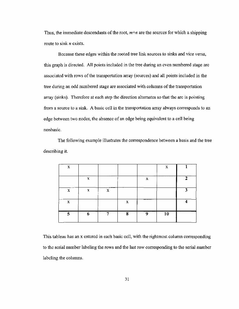
The following example illustrates the correspondence between a basis and the tree
describing it.
x x 1
x x 2
x x x 3
x x 4
5 6 7 8 9 10
This tableau has an x entered in each basic cell, with the rightmost column corresponding
to the serial number labeling the rows and the last row corresponding to the serial number
labeling the columns.
31
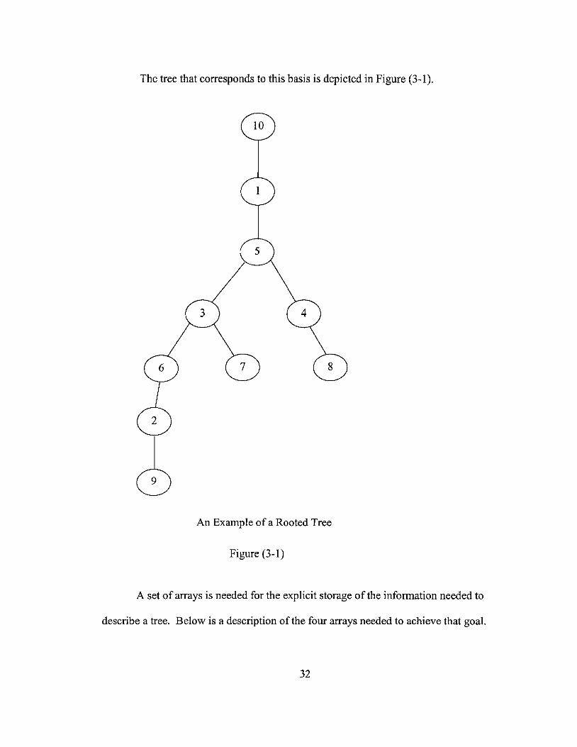
The tree that corresponds to this basis is depicted in Figure (3-1).
An Example of a Rooted Tree
Figure (3-1)
A set of arrays is needed for the explicit storage of the infonnation needed to
describe a tree. Below is a description of the four arrays needed to achieve that goal.
32
Choose node m+n as the root, then detennine all the row indices i such that
(m+n ; i) is an arc within the tree. Each such i is called a immediate successor (or child)
of m+n, and m+n is the predecessor of each such node. Predecessors and immediate
successors of other nodes are defined similarly. The notation for the predecessor index of
node} is P(j). If a node is a source, the predecessor index will be the serial number of a
sink and vice versa. If a node does not have a unique immediate successor, these
successors are considered brothers of each other, which are identified as a sequence
ranging from eldest to youngest. Designate the successor index of a node to be the eldest
son. Thus, for example if the younger brothers of node} are {h,j2' j3' ... ' jr}, then
designate S(j)= j! and the younger brother of jt to be jt+! for 1::;; t ::;; r-l, denoted as
YB(jJ=jt+!. The elder brother index is now self-explanatory. The notation for the elder
brother of} is EB(j) and for the previous example, EB(jt+!)=jt for 1::;; t ::;; r-I. If one of the
relationships does not exist for a certain node, the corresponding value is set to 0. For
example, for the root m+n, P(m+n)=O, YB(m+n)=O, and EB(m+n)=O. Also for any
tenninal node j, S(j)=O.
The set of younger brothers of} is the union of {YB(j)} and the set of younger
brothers ofYB(j). The set of immediate successors of a point} if S(j)*0 is the union of
{S(j)} and the set of the set of younger brothers of S(j). The descendants of i is the union
of the set of immediate successors of i and the sets of all descendants of} as} ranges over
the set of immediate successors of i. If i is a tenninal node, then the set of immediate
successors and descendents will be empty.
33
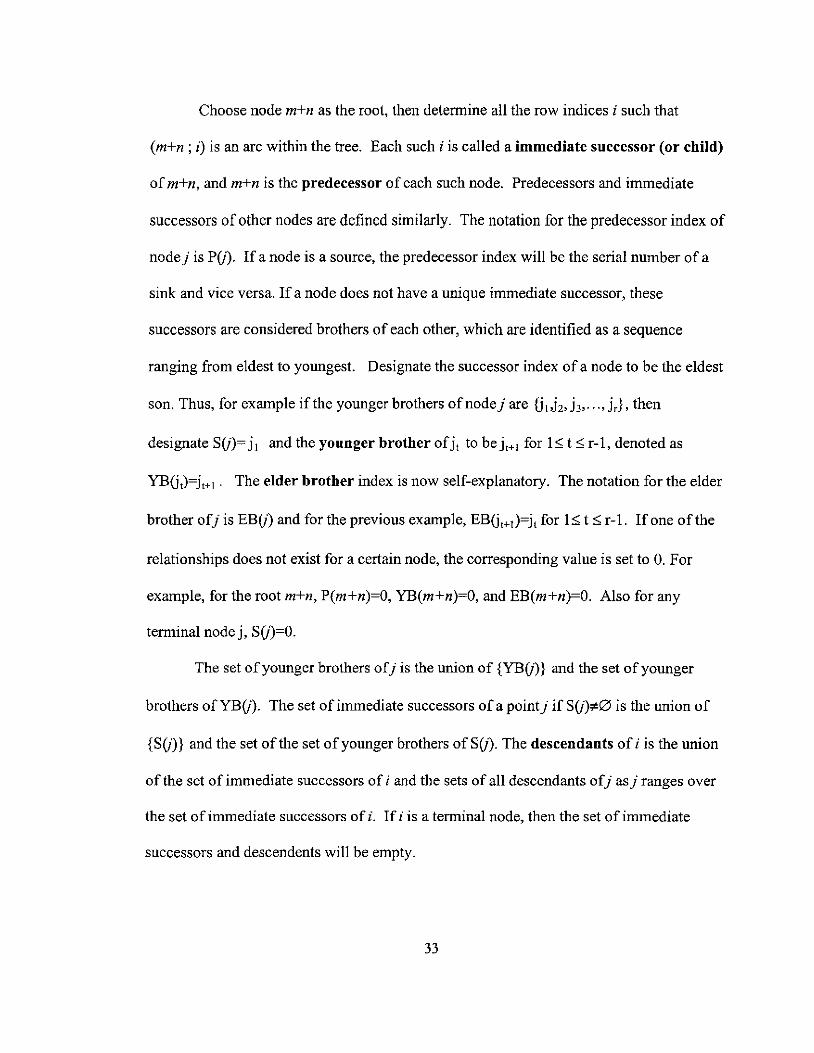
The predecessor, successor, younger brother, and the elder brother indices help
label the basis and are needed to alter the tree when a new basis is to be created.
Continuing with the previous example, the indices for the nodes obtained from the
current basis are as follows:
Nodes I 2 3 4 5 6 7 8 9 10
IPredecessor 10 6 5 5 I 3 3 4 2 0
Successor 5 9 6 8 3 2 0 0 0 I
Younger Brother 0 0 4 0 0 7 0 0 0 0
Elder Brother 0 0 0 3 0 0 6 0 0 0
Example of the Indices corresponding to a Rooted Tree
Figure (3-2)
Now we address the procedure of how to change a basis while using a tree as the
labeling method. The results of the following theorems are used to find a a-loop within
the tree.
Theorem (3.a). Let io and i. be a pair of points on a tree G. Then there exists a unique
simple path in G from io to i •.
Proof G is a tree so it is connected. Therefore there exists at least one path from io to i •.
If more than one path exists then combining these paths would create a cycle from io to io.
This contradicts the assumption of G being a tree .•
34
In the discussion below, L1 denotes a subset of cells.
Simple Cycles and 9-loops Theorem (3.b). Every 9-100p in L1 corresponds to a simple
cycle in G t!,. and vice versa.
Proof This follows from the definition of a loop and a simple cycle .•
Therefore L1 contains a 9-100p iff there is a simple cycle in Gt!,.. If At!,. contains m+n-I
edges, which is equivalent to a basis for the transportation array, it follows that Gt!,. is a
tree and therefore contains no cycles. This is equivalent to saying the tree contains no 9-
loops, which has already been proven for any basis of a transportation problem. Thus, L1
is a basis for the transportation array iff Gt!,.=(N,At!,.) is a tree.
The simple path between a point i and the root m+n is referred to as the
predecessor path of node i in GB (defined by the basis B) because only the predecessor
indices are used.
Definition: A simple path between a point and the root can be defined as follows:
1) The edge (i;P(i)) is the first edge in the path. IfP(i) is the root node, terminate.
Otherwise pick P(i) as the current point}.
2) (j;P(j)) is the next edge in the path.
3) IfP(j) is the root node, terminate. Otherwise, change the current point to P(j)
and return to step 2.
Let B be the basic set of cells for the transportation array and let (p,q) be the
nonbasic cell being introduced into the basis. The unique 9-100p in B u {(P,q)} can be
determined by the predecessor indices. The cell (p,q) corresponds to the emerging edge
35

(p;m+q) within the modified tree of the current graph GB. The 8-100p corresponds to the
simple cycle created when the edge (p;m+q) is included in graph, (N.ABU {(p;m+q)}).
To find the simple cycle, the unique simple path from m+q to the root node as
well as the unique simple path from p to the root node needs to be found. Eliminate all
common edges between these two simple paths. The last common point of these two
paths is known as the apex of the simple cycle. Combine what is left from both cycles to
create the simple cycle. When i is a node corresponding to a row index, the edges (i,j) in
this simple cycle correspond to the cells (ij-m) from the transportation array in the 8-
loop. Therefore once this simple cycle is found, the new basic feasible solution is formed
by adding +8 and -8 as described in chapter 2 and dropping one basic cell from the basis.
Assume the dropping cell is (r,s). Then the graph ofthe new basis B', GB " is obtained
from the graph GB by deleting the edge (r;m+s) and adding the edge (p;m+q).
To illustrate the modification of a tree, consider the example discussed earlier in
this chapter. Let the variable (3,6) be the variable selected to enter the basis and the
variable (3, I) be the variable leaving the basis (the dotted lines correspond to the loop).
The new tableau corresponding to this change is as follows:
x - ------- ------ ------- ------ x 1 I
X x 2
x x x 3 --- ------- ------- ------- ------- - --
x x 4
5 6 7 8 9 10
36
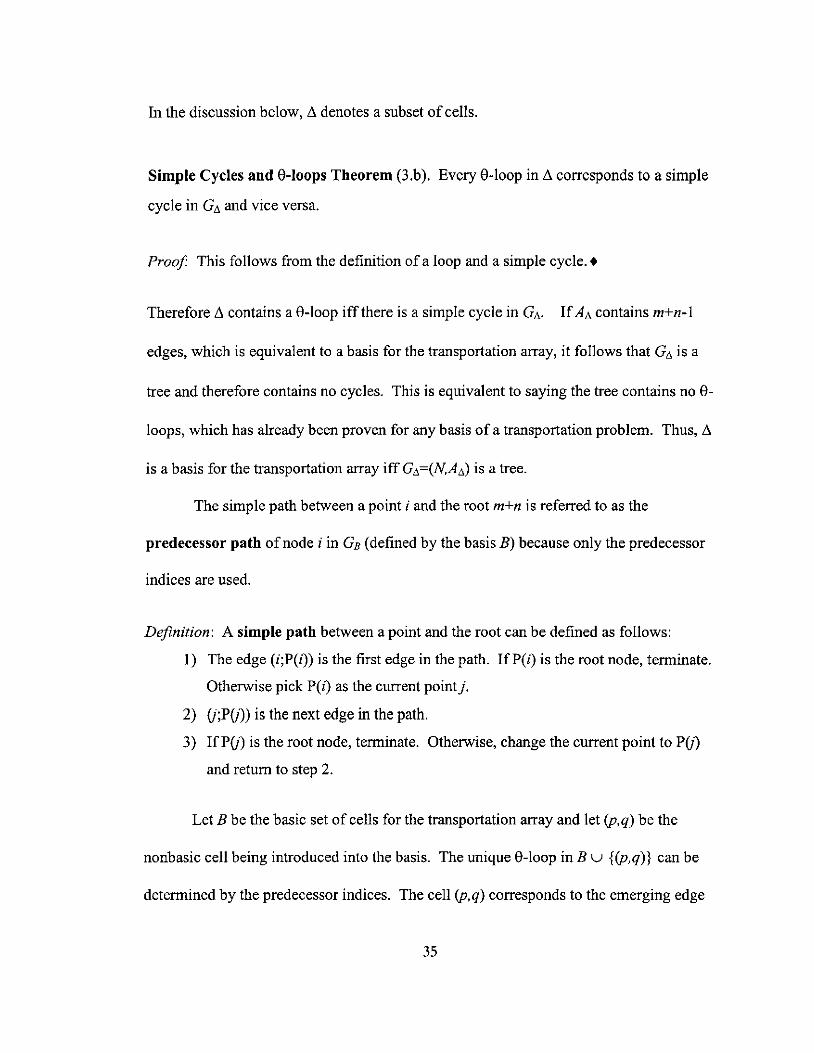
The modifying ofthe tree in Figure (3-2) corresponding to this new basis is as
follows:
o I I
I I
I I I
I I
I I
I I
I I I
I I I
I I I
I I I I I I
I I I
I I
I I
Example of Dropping and Entering Edge ofa Tree
Figure (3-3)
The dashed line represents the entering edge and the edge that is slashed represents the
edge that is being removed.
37
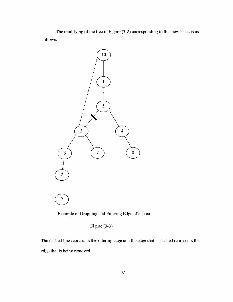
Figure (3-4) displays the modified tree that fits the new basis.
Example of a Modified Tree
Figure (3-4)
38
Chapter 4
SOME IMPLEMENTATION DETAILS
The computer program used to solve the transportation problem essentially
follows the steps of the transportation algorithm outlined in the previous chapters. In this
chapter, we outline some ofthe implementation details. Not all the subroutines will be
discussed because there is extensive documentation within the program.
The sparsity of the transportation array, x, is an obvious problem that needs to be
addressed; Only m +n-l entries can be nonzero while x contains mn entries. In this
program, a special method was used to store this matrix. The m+n-l basic variables are
stored in a linear array X. Thus, X(l), X(2), ... , X(m+n-l) will always contain the basic
variables, arranged by rows. In the vector ROW, the ith entry contains the location in X
of the first basic entry from the ith row forI$; i$; n, and in the vector COL, the /h entry
contains the column index of the basic variables XU) for l$;j$; m+n-l. This allows the
program to store the basic feasible solutions more efficiently, since the rest ofthe values
within the matrix x are O. This method of storage does complicate the program, but the
memory space saved by this method far out weighs the expense of adding these pieces.
39

The following is an example of how the basis is stored.
1 4
3 2
6 8 7
9 12
I 1 2 3 4 5 6 7 8 9 X 1 4 3 2 6 8 7 9 12
Column 1 6 2 5 1 2 3 1 4
I 1 2 3 4
Row 1 3 5 8
For example, if we want to find the value ofthe basic variable xij' the entries
COL(k) should be scanned for Row(i)::; k::; ROW(i+ 1 )-1, until COL(k)=). Subroutine
FIND performs this task and can be found on page 61. It will output the index value of
where the basic variable is located within X.
The first step of this program is to find an initial basic feasible solution to the
primal. This is done using the Northwest Comer Rule and is performed by the subroutine
NW, found on page 54. The design of this method makes it easier to program than other
methods. The entries of COL(j) and X(j) are recorded at each step in the order in which
the basic variables are allocated, while the value ofthe ith entry in ROW(i) is assigned)
when the first entry of the ith row is assigned. The program will print a statement
signaling that the problem is degenerate, if a value of 0 is assigned to any of the basic
40

variables. Once the initial basic feasible solution is found, the initial cost is calculated
and stored. As discussed earlier, when a new basic feasible solution is found, adding the
reduced cost of the entering variable multiplied by 8 gives the cost ofthe new solution.
An important step of this algorithm is to determine if the solution obtained is
optimal. This is where the computer algorithm differs from the hand calculation
algorithm. Trees need to be introduced so that a 8-100p can be determined easily. The
initial rooted tree is created using the subroutine TREE located on page 56 and 57. The
predecessor, successor, younger brother, and elder brother indices of each node (j= 1 to
m+n-l) are saved in the following vectors respectively: PRED(j), SUCC(j), YB(j), and
EB(j). The successor index saves the serial number of the eldest son. The younger
brother index saves the serial number of the eldest among the set of younger brothers and
the eldest brother index saves the serial number of the youngest among the set of the
eldest brothers. In order to keep track of which nodes have been labeled so far, a vector
SLIST is used. SLIST is initially set so that the ilh entry equals i, for i=l to m+n-l.
Once a node has been labeled, the entry corresponding to its serial number in SLIST is
changed to o. The vector NODE is used to store the nodes, which need to be processed at
a later stage. The value of the variable KOUNTER is the number of the node currently
being processed.
If KOUNTER is a source node, then the column indices associated with the
successors of KOUNTER are known because of the way that X is stored. If the node
corresponding to the column has not already been processed, its predecessor index is
defined to be equal to the KOUNTER. If there is more than one column that corresponds
to this row and they have not been processed yet, these will be brothers, letting the eldest
41
brother correspond to the first column obtained and the youngest brother correspond to
the last. The same process is carried out if KOUNTER corresponds with a column index,
except that the location of the row indices, corresponding to the basic cells in that
column, must be determined. This process is repeated until each node is labeled. If a
node does not have one of these indices, it is labeled as a O.
The first step of the main loop of this program is to determine if all reduced costs
are positive, and, if not, to determine the entering variable into the basis. This is done by
the subroutine NEWBAS, which is located on page 58. NEWBAS is designed to pick
the new variable to enter the basis using the modified row first negative method. This
method was used because a study published in "Management Science" in 1974 showed
that this method was most efficient, taking into consideration the time it takes to find the
pivot variable, the average time per pivot, and the total pivot time (Glover, pg. 801).
Modified Row First Negative Method finds the first row with a negative cost coefficient
and then scans the rest of that row for any smaller reduced cost, saving the smallest. It
saves the row index of the variable entering the basis as NBR, and the column index of
the variable entering the basis as NBC. If all reduced costs are nonnegative, this solution
is optimal, and the program terminates. If not, the program will print the iteration
number and what variable is entering the basis.
The next step in the main iteration loop is to find the 8-loop using the rooted tree.
This is done within the subroutine QLOOP on page 59 and 60. In order to do this, the
simple path from P= NBR to the root and the simple path from Q= NBC+m to the root
must be found. These simple paths are found by starting with P or Q, and moving up the
tree using the predecessor indices until the root is reached (saving the nodes along the
42
path). PPATH has a designated first entry ofNER and the rest of the entries correspond
to the nodes contained in the simple path between P= NER and the root. QP ATH' s first
two entries correspond to NBR and NBC+m, respectively. After these first two entries,
the nodes in the simple path between Q = NBC+m and the root are stored, with the last
entry being the root. After these two paths are determined, they are combined within
QP ATH, eliminating any duplicated nodes contained within each path except for the
APEX of this cycle. At the end of this subroutine, QP ATH contains the simple cycle
from P=NBR to Q = NBC and PPATH contains the simple path from P = NBR to the
APEX.
Now that the e-Ioop has been found and stored within QPATH, the value ofe
must be determined, and X must be modified. The subroutine MODFYX on page 62 and
63, performs these operations. In this subroutine, lIN = NBR and JIN = NBC. The first
step of determining the value of e is to determine the donor and the recipient cells.
Because of the way QP ATH was constructed and because the tree is a directed graph, the
nodes will correspond alternately to a row and a column index, allowing the variables
corresponding to the basis to easily be determined. The first two entries within QP ATH
were defined so that they would correspond to the row and the column of the variable
entering the basis. Starting with the third entry, the first basic variable ofthe loop is equal
to X(QPATH(3), QPATH(2)-m), and corresponds to a donor cell. For i=3 and
subsequent odd indices to the end of the array, the next two basic variables are X(
QPATH(i), QPATH(i+ l)-m), corresponding to a recipient cell and X(QPATH(i+2),
QPATH(i+l)-m), corresponding to a donor cell. With the row and column indices
known, each basic variable must be found within the X vector using the FIND subroutine.
43
Once it is found, the location of where it is located within COL and X is saved within
LIST. The minimum value of X for donor cell is saved as THETA, and the row index as
lOUT, the column index as lOUT, and the location of where the cell is within X as
IDROP. Then THETA is subtracted from the donor cells and added to the recipient cells,
which can be done easily because the location of each cell was saved within LIST
(alternating donor and recipient).
Now the variable leaving the basis must be removed from X and the entering
variable must be added. Because of the way that the basic variables were saved in X, it
must be decided if the row of the cell entering is greater than the row ofthe cell that is
leaving. The entering variable will be listed at the beginning of the section of COL and
X, corresponding to its row. If lIN> lOUT, the indices in COL and X need to be
shifted to the left. Otherwise, the indices in COL and X need to be shifted to the right.
The indices are only altered between the rows of the entering and the leaving variables.
Once the X values have been modified, RLEFT is given the value of the row and
CLEFT is given the value of the column of the variable leaving the basis. The rest of the
program is well documented in the following chapter.
44
Chapter 5
FORTRAN CODE FOR THE TRANSPORTATION PROBLEM
!***********************************************************************************************
!OPTRAN IS A PROGRAM THAT CALCULATES THE OPTIMAL SOLUTION FOR A !TRANSPORTATION PROBLEM !*************************************************************************************
PROGRAM OPTTRAN PARAMETER (M=l OOO,N=1000) INTEGER A(M), B(N), C(M,N), X(M+N-l), U(M), V(N), THETA, COST INTEGER ROW(M+l), COL(M+N-l), RLEFT, CLEFT, RROW, ROOT INTEGER PRED(M+N), SUCC(M+N), EB(M+N), YB(M+N), INTEGER NINJC(N), NINJR(M), RINJS(M), CINJS(N) INTEGER DESJSTAR(M+N), ALPHA, NDESJSTAR(M+N) INTEGER QPATH(M+N+l), PPATH(M+N+l), JPATH(M+N), RED COST REAL A VLENDJ
X=O ROW=O COL=O U=O V=O NBR=O NBC=O KSTOP=l COST=O ROW(M+l)=M+N
!************************************************************************************* !CALCULATING A COST MATRIX, A,B FOR A TEST PROBLEM WHICH CREATES THE !OPTIMAL SOLUTION TO BE CREATED BY THE SOUTHEAST CORNER RULE
M= # OF SOURCES N= #OFSINKS C= COST MATRIX A= V ALUE AVAILABLE FROM SOURCE B= VALUE NEEDED AT SINK
!*************************************************************************************
CALL CREATE(M,N,C,A,B)
45
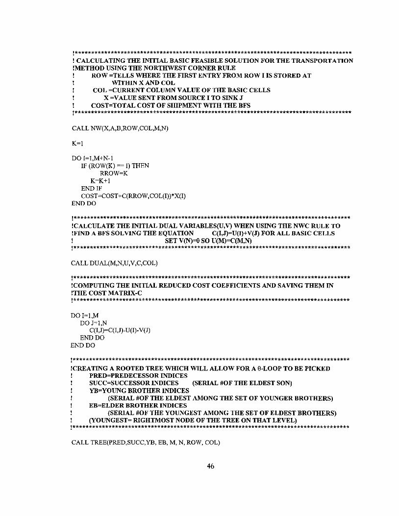
!************************************************************************************* ! CALCULATING THE INITIAL BASIC FEASIBLE SOLUTION FOR THE TRANSPORTATION !METHOD USING THE NORTHWEST CORNER RULE
ROW =TELLS WHERE THE FIRST ENTRY FROM ROW I IS STORED AT WITIDN X AND COL
COL =CURRENT COLUMN VALUE OF THE BASIC CELLS X =V ALUE SENT FROM SOURCE I TO SINK J
COST=TOTAL COST OF SHIPMENT WITH THE BFS !*************************************************************************************
CALL NW(X,A,B,ROW,COL,M,N)
K=l
DO I=l,M+N-l IF (ROW(K) == I) THEN
RROW=K K=K+l
END IF COST=COST +C(RROW,COL(I»*X(I)
END DO
!************************************************************************************* !CALCULATE THE INITIAL DUAL V ARIABLES(U,V) WHEN USING THE NWC RULE TO !FIND A BFS SOLVING THE EQUATION C(I,J)=U(I)+V(J) FOR ALL BASIC CELLS
SET V(N)=O SO U(M)=C(M,N) !*************************************************************************************
CALL DUAL(M,N,U,V,C,COL)
!************************************************************************************* !COMPUTING THE INITIAL REDUCED COST COEFFICIENTS AND SAVING THEM IN !THE COST MATRlX-C !*************************************************************************************
DO I=l,M DO J=l,N
C(I,J)=C(I,J)-U (1)-V (J) END DO
END DO
!************************************************************************************* !CREATING A ROOTED TREE wmCH WILL ALLOW FOR A 8-LOOP TO BE PICKED
PRED=PREDECESSORINDICES SUCC=SUCCESSOR INDICES (SERIAL #OF THE ELDEST SON) YB=YOUNG BROTHER INDICES
(SERIAL #OF THE ELDEST AMONG THE SET OF YOUNGER BROTHERS) EB=ELDER BROTHER INDICES
(SERIAL #OF THE YOUNGEST AMONG THE SET OF ELDEST BROTHERS) (YOUNGEST= RIGHTMOST NODE OF THE TREE ON THAT LEVEL)
!*************************************************************************************
CALL TREE(PRED,SUCC,YB, EB, M, N, ROW, COL)
46

!************************************************************************************* !START OF LOOP TO FIND OPTIMAL SOLUTIONHAVE BASIC FEASIBLE SOLN,
NEED DUAL TO ALSO BE FEASIBLE SO NEED ALL REDUCED COSTS> 0 KOUNT=KEEPS TRACK OF HOW MANY ITERATIONS KSTOP=WHEN ALL RC>O TillS IS SET TO 0 SO THAT IT EXITS LOOP
!*************************************************************************************
KOUNT=1
DO WHILE (KSTOP = 1) !BEGINNING OF LARGE LOOP
!************************************************************************************* !PICKING THE NEW VARIABLE TO ENTER THE BASIS USING MODIFIED ROW FIRST !NEGATIVE METHOD. TillS METHOD FINDS THE FIRST ROW WITH A NEG REDUCED !COST COEFFICIENT AND THEN SCANS THE REST OF THAT ROW FOR ANY OTHER RC !WHICH IS MORE NEGATIVE.
NBR= ROW OF VARIABLE ENTERING THE BASIS NBC= COLUMN OF VARIABLE ENTERING THE BASIS
!*************************************************************************************
CALL NEWBAS(M,N,C,NBR,NBC,KSTOP)
IF (KSTOP = 0) THEN GO TO 1000
END IF
!EXIT LOOP IF OPTIMAL
PRINT *, 'AT ITERA TION',KOUNT " THE ENTERING VARIABLE INTO THE BASIS IS' PRINT *, 'XC, NBR, NBC,')'
!************************************************************************************* !THIS FINDS THE 8-LOOP USING THE ROOTED TREE WITH THE NONBASIC !CELL(P,Q)=(NBR,NBC) TO ENTER THE BASIS. IN ORDER TO DO THIS -THE SIMPLE !PATH FROM P TO THE ROOT(M+N) AND THE SIMPLE PATH FROM Q(M+Q) TO THE !ROOT MUST BE FOUND. THEN WE COMBINE THESE TWO PATHS ELIMINATING ANY !DUPLICATES, LEAVING ONLY ONE DUPLICATE, WHICH IS THE APEX.
QPATH= SIMPLE PATH FROM Q TO THE ROOT AT END- SIMPLE CYCLE FROM P TO Q
LENQ= LENGTH OF QPATH PPATH= SIMPLE PATH FROM P TO ROOT
AT END- SIMPLE PATH FROM P TO APEX LENP= LENGTH OF PATHOFP
!*************************************************************************************
CALL QLOOP(NBR,NBC,QPATH,M,N,PRED,LENQ,LENP,PPA TH)
47

!************************************************************************************* !THIS CHANGES THE VALUE OF X (THE BASIS) - ADD e TO RECIPIENT CELLS AND !SUBTRACT e FROM THE DONOR CELLS. CHANGE THE NONBASIC TO A BASIC CELL.
IDROP= POSITION OF THE BASIC CELL WHICH IS LEAVING THE BASIS RLEFT=ROW INDEX OF CELL LEAVING THE BASIC FEASIBLE SOLN CLEFT=COLUMN INDEX OF CELL LEAVING THE BASIC FEASIBLE SOLN THETA= VALUE OF NEW BASIC CELL/OLD BASIC CELL
!*************************************************************************************
CALL MODFYX(QP A TH,LENQ,M,N,X,ROW,COL,IOUT,IDROP,JOUT, THETA) CLEFT=JOUT RLEFT=IOUT
PRINT *, 'THETA=', THETA
!************************************************************************************* !THIS IS THE BEGINNING OF UPDATING THE ROOTED TREE
RINJS= THE ROW INDICES CONTAINED AS A DESCENDANT OF J* CINJS= THE COLUMN INDICES CONTAINED AS A DESCENDANT OF J* LENR=LENGTH OF RINJS LENC=LENGTH OF CINJS (I1;Jl) IS THE EDGE THAT IS ADDED (I2;JSTAR) IS THE EDGE THAT IS LEAVING I2=PRED(JSTAR) ALPHA= USED LATER FOR CHANGING RC COEFFICIENTS KTESTER=KEEPS TRACK OF IF 12,J* ARE ON PPATH TO THE APEX
!*************************************************************************************
RINJS=O CINJS=O LENC=O LENR=O
IF (PRED(RLEFT) = CLEFT+M) THEN JSTAR=RLEFT I2=CLEFT+M RINJS(1)=JSTAR LENR=1
ELSE JSTAR=CLEFT+M I2=RLEFT CINJS(l)=JSTAR-M LENC=1
END IF
KTESTER=O IV=1
48
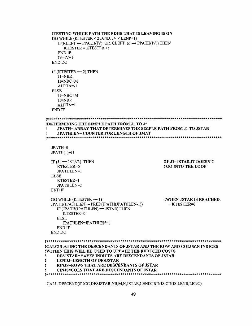
!TESTING WHICH PATH THE EDGE THAT IS LEAVING IS ON DO WHILE (KTESTER < 2 .AND. IV < LENP+ 1)
IF(RLEFT == PPATH(IV) .OR. CLEFT+M = PPATH(IV» THEN KTESTER = KTESTER + 1
END IF IV=IV+l
END DO
IF (KTESTER = 2) THEN Jl=NBR I1=NBC+M ALPHA=-l
ELSE Jl=NBC+M I1=NBR ALPHA=l
END IF
!************************************************************************************* !DETERMINING THE SIMPLE PATH FROM Jl TO J*
JPATH= ARRAY THAT DETERMINES THE SIMPLE PATH FROM Jl TO JSTAR JPATHLEN= COUNTER FOR LENGTH OF JMAT
!*************************************************************************************
JPATH=O JPATH(l)=Jl
IF (Jl = JSTAR) THEN KTESTER=O JPATHLEN=l
ELSE KTESTER=l JPATHLEN=2
END IF
DO WHILE (KTESTER = 1) JPATH(JPATHLEN) = PRED(JPATH(JPATHLEN-l»
IF (JPATH(JPATHLEN) == JSTAR) THEN KTESTER=O
ELSE JP ATHLEN=JP A THLEN+ 1
END IF END DO
!IF Jl=JSTAR,IT DOESN'T ! GO INTO THE LOOP
!WHEN JSTAR IS REACHED, ! KTESTER=O
!************************************************************************************* !CALCULATING THE DESCENDANTS OF JSTAR AND THE ROW AND COLUMN INDICES !WITHIN THIS WILL BE USED TO UPDATE THE REDUCED COSTS
DESJST AR= SAVES INDICES ARE DESCENDANTS OF JST AR LENDJ=LENGTH OF DESJST AR RINJS=ROWS THAT ARE DESCENDANTS OF JSTAR CINJS=COLS THAT ARE DESCENDANTS OF JSTAR
!*************************************************************************************
CALL DESCEND(SUCC,DESJSTAR,YB,M,N,JSTAR,LENDJ,RINJS,CINJS,LENR,LENC)
49
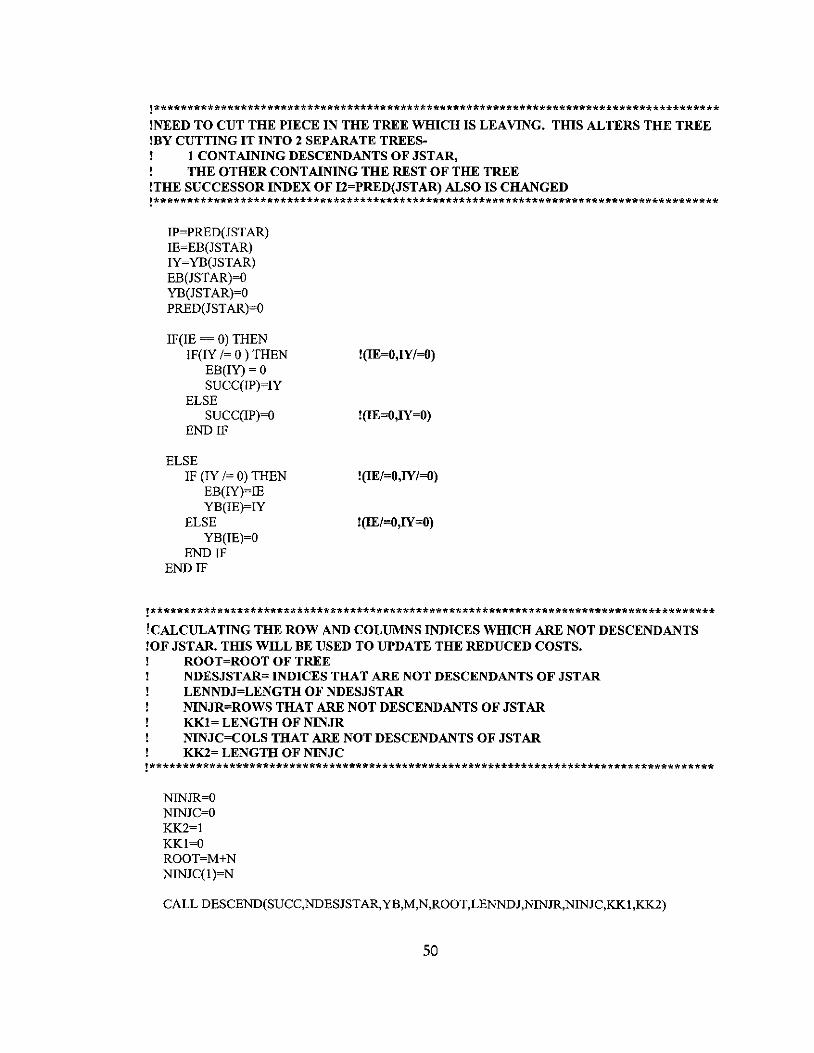
!************************************************************************************* !NEED TO CUT THE PIECE IN THE TREE WHICH IS LEAVING. THIS ALTERS THE TREE !BY CUTTING IT INTO 2 SEPARATE TREES-
1 CONTAINING DESCENDANTS OF JSTAR, THE OTHER CONTAINING THE REST OF THE TREE
!THE SUCCESSOR INDEX OF I2=PRED(JSTAR) ALSO IS CHANGED !*************************************************************************************
IP=PRED(JSTAR) IE=EB(JSTAR) IY=YB(JSTAR) EB(JSTAR)=O YB(JSTAR)=O PRED(JST AR)=O
IF(IE = 0) THEN IF(IY /= 0 ) THEN
EB(IY) = 0 SUCC(IP)=IY
ELSE SUCC(IP)=O
END IF
ELSE IF (IY /= 0) THEN
EB(IY)=IE YB(IE)=IY
ELSE YB(IE)=O
END IF END IF
!(lE=O,IY /=0)
!(lE=O,IY=O)
!(IE/=O,JY/=O)
!(IE/=O,JY=O)
!************************************************************************************* !CALCULATING THE ROW AND COLUMNS INDICES WHICH ARE NOT DESCENDANTS !OF JSTAR. THIS WILL BE USED TO UPDATE THE REDUCED COSTS.
ROOT=ROOT OF TREE NDESJSTAR= INDICES THAT ARE NOT DESCENDANTS OF JSTAR LENNDJ=LENGTH OF NDESJSTAR NINJR=ROWS THAT ARE NOT DESCENDANTS OF JSTAR KKl= LENGTH OF NINJR NINJC=COLS THAT ARE NOT DESCENDANTS OF JSTAR KK2= LENGTH OF NINJC
!*************************************************************************************
NINJR=O NINJC=O KK2=1 KKl=O ROOT=M+N NINJC(l)=N
CALL DESCEND(SUCC,NDESJSTAR,YB,M,N,ROOT,LENNDJ,NINJR,NINJC,KKl,KK2)
50
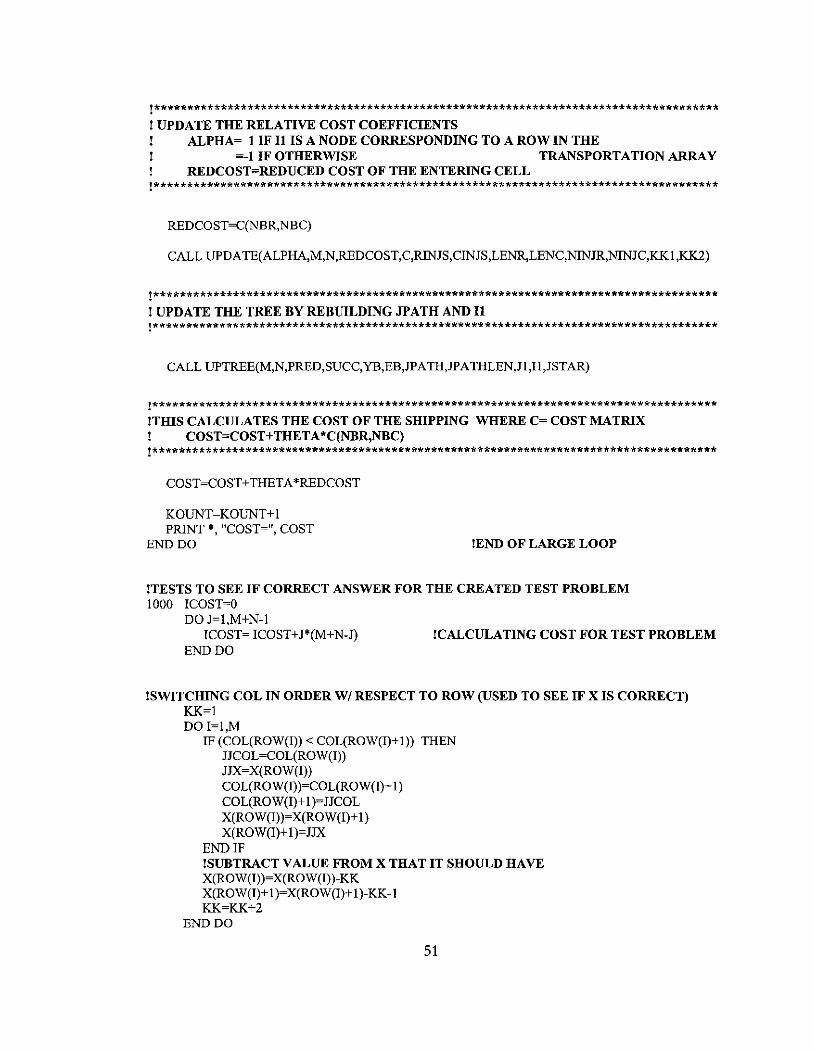
!************************************************************************************* ! UPDATE THE RELATIVE COST COEFFICIENTS
ALPHA= 1 IF It IS A NODE CORRESPONDING TO A ROW IN THE =-1 IF OTHERWISE TRANSPORTATION ARRAY
REDCOST=REDUCED COST OF THE ENTERING CELL !*************************************************************************************
REDCOST=C(NBR,NBC)
CALL UPDA TE(ALPHA,M,N,REDCOST,C,RINJS,CINJS,LENR,LENC,NINJR,NINJC,KK1 ,KK2)
!************************************************************************************* ! UPDATE THE TREE BY REBIDLDING JPATH AND It !*************************************************************************************
CALL UPTREE(M,N,PRED,SUCC,YB,EB,JP A TH,JP A THLEN,n ,I1,JSTAR)
!************************************************************************************* !THIS CALCULATES THE COST OF THE SIDPPING WHERE C= COST MATRIX
COST=COST+THETA*C(NBR,NBC) !*************************************************************************************
COST=COST+THETA*REDCOST
KOUNT=KOUNT + 1 PRINT *, "COST=", COST
END DO !END OF LARGE LOOP
!TESTS TO SEE IF CORRECT ANSWER FOR THE CREATED TEST PROBLEM 1000 ICOST=O
DO J=1,M+N-1 ICOST= ICOST+J*(M+N-J) !CALCULATING COST FOR TEST PROBLEM
END DO
!SWITCIDNG COL IN ORDER WI RESPECT TO ROW (USED TO SEE IF X IS CORRECT) KK=1 DO I=l,M
IF (COL(ROW(I)) < COL(ROW(I)+l» THEN nCOL=COL(ROW(l)) JJX=X(ROW(l)) COL(ROW(I))=COL(ROW(I)+ 1) COL(ROW(I)+ 1)= nCOL X(ROW(l))=X(ROW(I)+ 1) X(ROW(I)+1)=JJX
END IF !SUBTRACT VALUE FROM X THAT IT SHOULD HAVE X(ROW(I))=X(ROW(I))-KK X(ROW(I)+ l)=X(ROW(I)+ l)-KK-l KK=KK+2
END DO
51
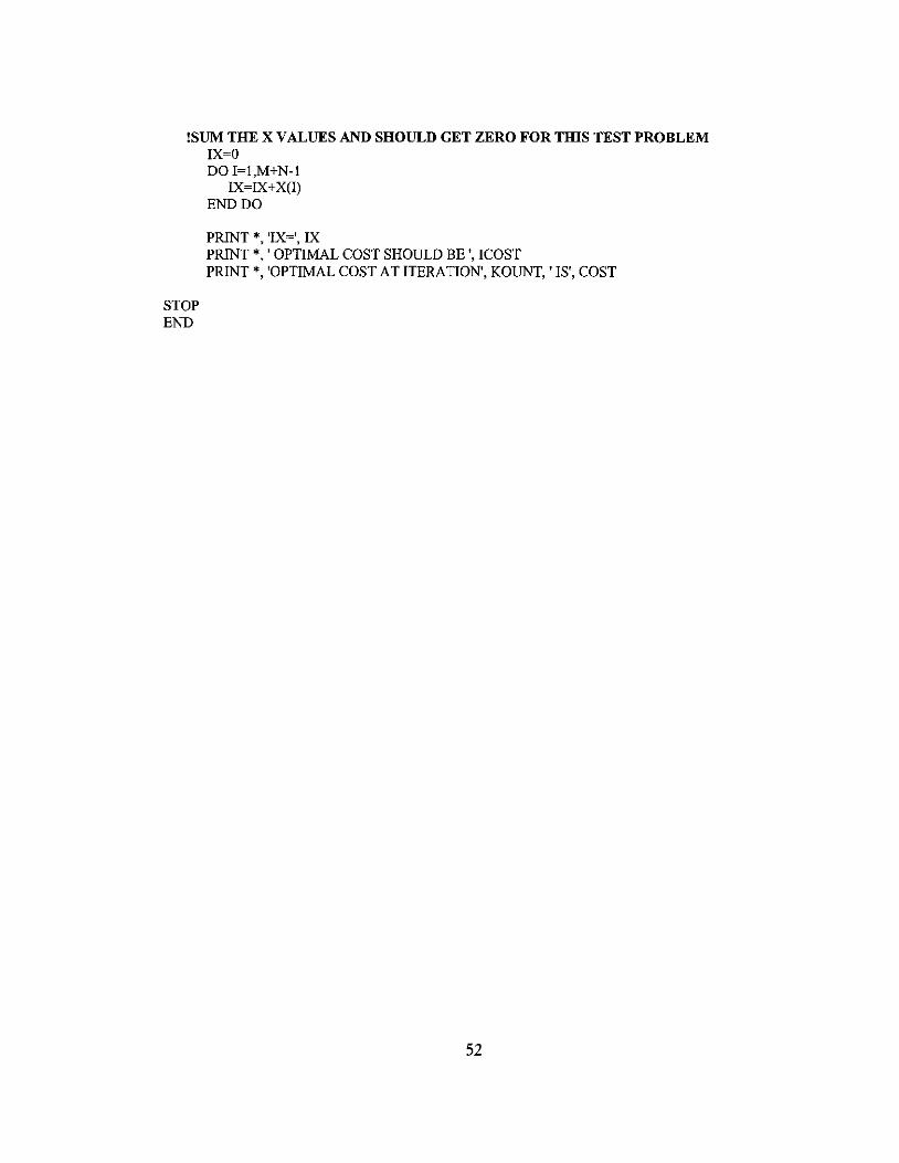
!SUM THE X VALUES AND SHOULD GET ZERO FOR TIDS TEST PROBLEM IX=O
STOP END
DO I=l,M+N-l IX=IX+X(I)
END DO
PRINT *, 'IX=', IX PRINT *, 'OPTIMAL COST SHOULD BE " ICOST PRINT *, 'OPTIMAL COST AT ITERATION', KOUNT, 'IS', COST
52
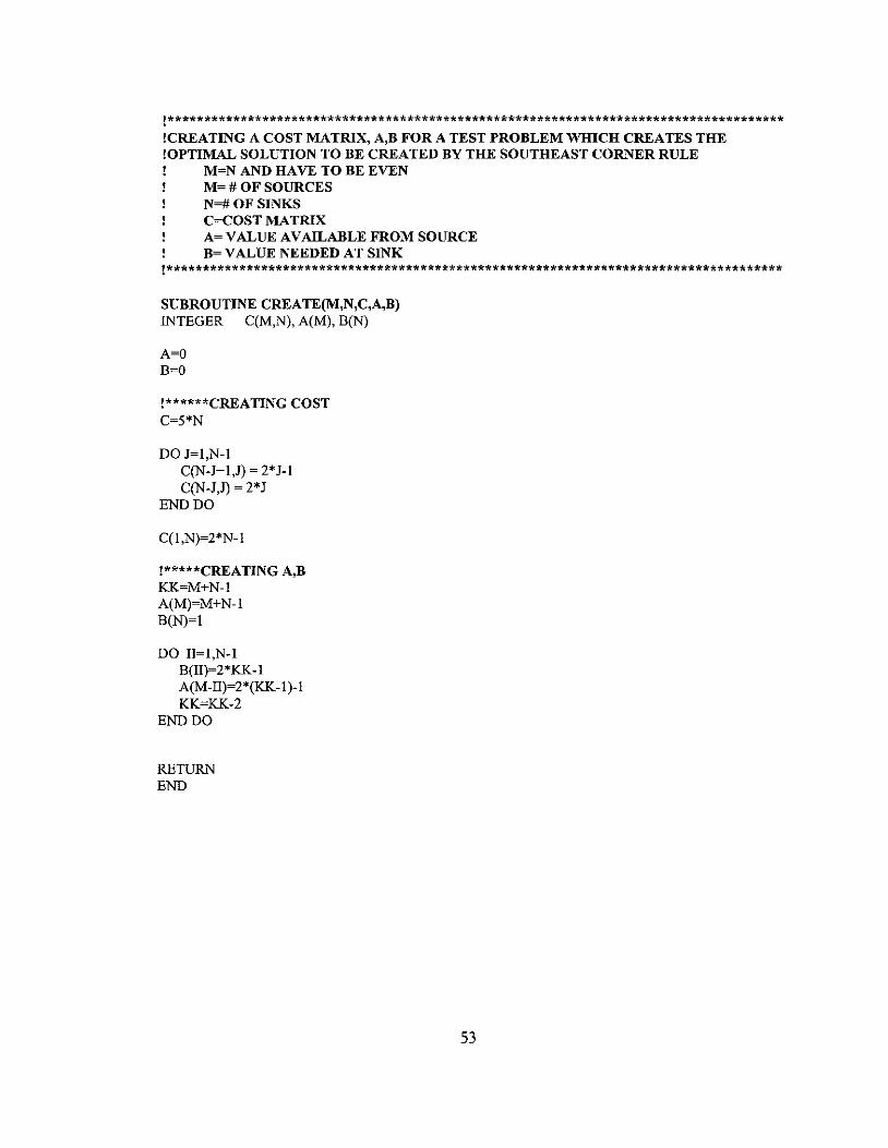
!************************************************************************************* !CREATING A COST MATRIX, A,B FOR A TEST PROBLEM WHICH CREATES THE !OPTIMAL SOLUTION TO BE CREATED BY THE SOUTHEAST CORNER RULE
M=N AND HAVE TO BE EVEN M= # OF SOURCES N=# OF SINKS C=COST MATRIX A= VALUE AVAILABLE FROM SOURCE B= VALUE NEEDED AT SINK
!*************************************************************************************
SUBROUTINE CREATE(M,N,C,A,B) INTEGER C(M,N), A(M), B(N)
A=O B=O
!******CREATING COST C=5*N
DO J=1,N-1 C(N-J+1,J) = 2*J-1 C(N-J,J) = 2*J
END DO
C(1,N)=2*N-1
!*****CREATING A,B KK=M+N-1 A(M)=M+N-1 B(N)=l
DO II=1,N-1 B(II)=2*KK-1 A(M-II)=2*(KK-1)-1 KK=KK-2
END DO
RETURN END
53
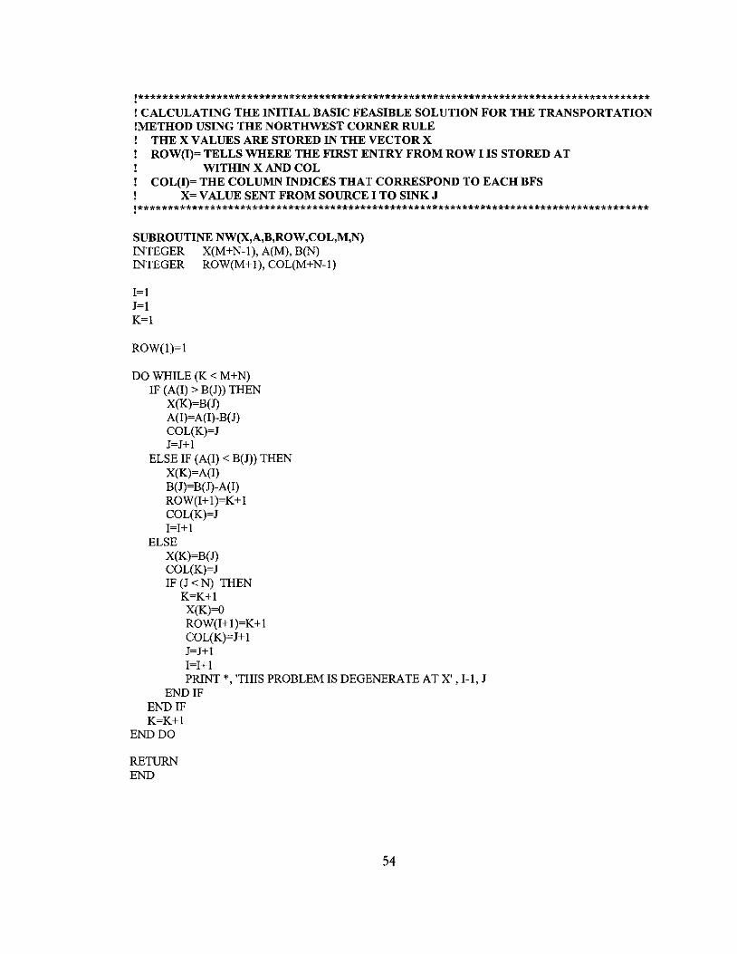
!************************************************************************************* ! CALCULATING THE INITIAL BASIC FEASIBLE SOLUTION FOR THE TRANSPORTATION !METHOD USING THE NORTHWEST CORNER RULE
THE X VALUES ARE STORED IN THE VECTOR X ROW{I)= TELLS WHERE THE FIRST ENTRY FROM ROW I IS STORED AT
WITHIN X AND COL COL(I)= THE COLUMN INDICES THAT CORRESPOND TO EACH BFS
X= VALUE SENT FROM SOURCE I TO SINK J !*************************************************************************************
SUBROUTINE NW(X,A,B,ROW,COL,M,N) INTEGER X(M+N-l), A(M), B(N) INTEGER ROW(M+1), COL(M+N-l)
1=1 J=1 K=1
ROW(I)=1
DO WHILE (K < M+N) IF (A(I) > B(J» THEN
X(K)=B(J) A(I)=A(I)-B(J) COL(K)=J J=1+1
ELSE IF (A(I) < B(J» THEN X(K)=A(I) B(J)=B(J)-A(I) ROW(l+l)=K+l COL(K)=J 1=1+1
ELSE X(K)=B(J) COL(K)=J IF (J < N) THEN
K=K+l X(K)=O ROW(I+ 1 )=K + 1 COL(K)=1+1 J=1+1 1=1+1 PRINT *, 'THIS PROBLEM IS DEGENERATE AT X' ,1-1, J
END IF END IF K=K+l
END DO
RETURN END
54
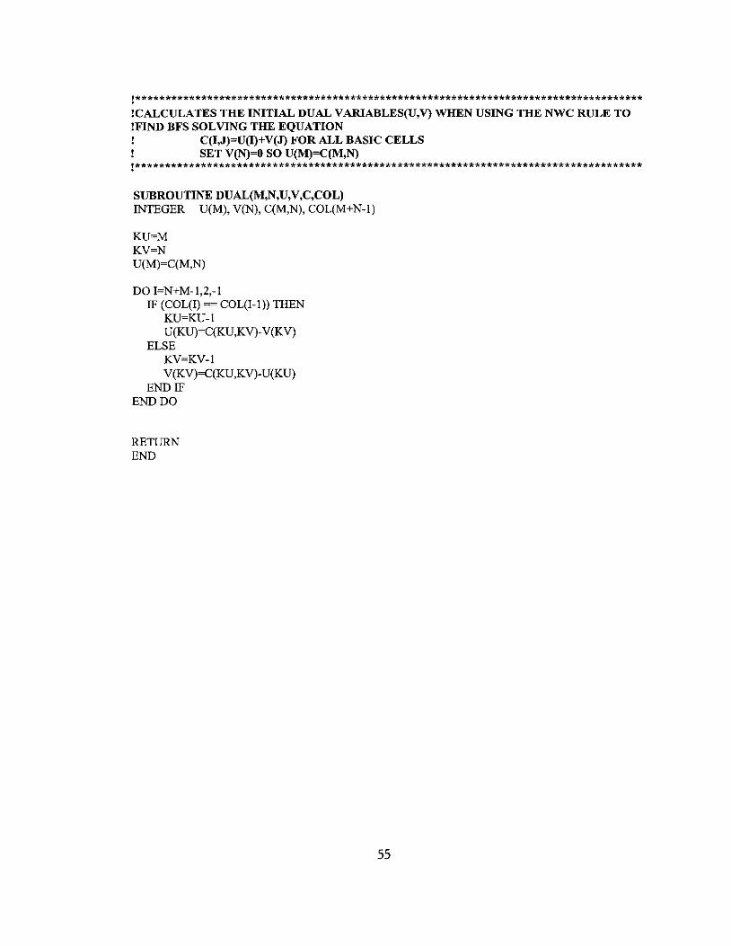
!************************************************************************************* !CALCULATES THE INITIAL DUAL V ARlABLES(U,V) WHEN USING THE NWC RULE TO !FIND BFS SOLVING THE EQUATION
C(I,J)=U(I)+V(J) FOR ALL BASIC CELLS SET V(N)=O SO U(M)=C(M,N)
!*************************************************************************************
SUBROUTINE DUAL(M,N,U,V,C,COL) INTEGER U(M), V(N), C(M,N), COL(M+N-I)
KU=M KV=N U(M)=C(M,N)
DO I=N+M-I,2,-1 IF (COL(I) = COL(I-I)) THEN
KU=KU-I U(KU)=C(KU,KV)-V(KV)
ELSE KV=KV-I V(KV)=C(KU,KV)-U(KU)
END IF END DO
RETURN END
55
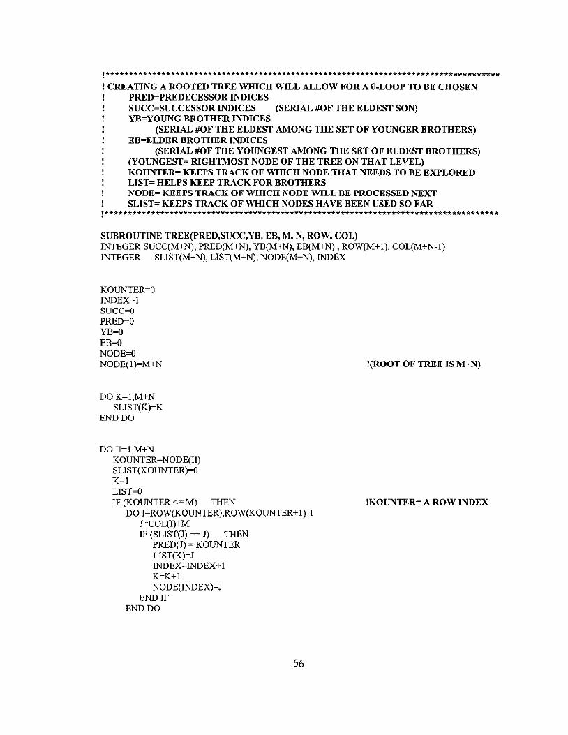
!************************************************************************************* ! CREATING A ROOTED TREE WHICH WILL ALLOW FOR A 8-LOOP TO BE CHOSEN
PRED=PREDECESSOR INDICES SUCC=SUCCESSOR INDICES (SERIAL #OF THE ELDEST SON) YB=YOUNG BROTHER INDICES
(SERIAL #OF THE ELDEST AMONG THE SET OF YOUNGER BROTHERS) EB=ELDER BROTHER INDICES
(SERIAL #OF THE YOUNGEST AMONG THE SET OF ELDEST BROTHERS) (YOUNGEST= RIGHTMOST NODE OF THE TREE ON THAT LEVEL) KOUNTER= KEEPS TRACK OF WHICH NODE THAT NEEDS TO BE EXPLORED LlST= HELPS KEEP TRACK FOR BROTHERS NODE= KEEPS TRACK OF WHICH NODE WILL BE PROCESSED NEXT SLlST= KEEPS TRACK OF WHICH NODES HAVE BEEN USED SO FAR
!*************************************************************************************
SUBROUTINE TREE(PRED,SUCC,YB, EB, M, N, ROW, COL) INTEGER SUCC(M+N), PRED(M+N), YB(M+N), EB(M+N), ROW(M+1), COL(M+N-1) INTEGER SLIST(M+N), LIST(M+N), NODE(M+N), INDEX
KOUNTER=O INDEX=1 SUCC=O PRED=O YB=O EB=O NODE=O NODE(1 )=M+N
DOK=1,M+N SLIST(K)=K
END DO
DO II=1,M+N KOUNTER=NODE(II) SLIST(KOUNTER)=O K=1 LIST=O IF (KOUNTER <= M) THEN
DO I=ROW(KOUNTER),ROW(KOUNTER+ 1 )-1 J=COL(I)+M IF (SLIST(J) = 1) THEN
PRED(J) = KOUNTER LIST(K)=J INDEX=INDEX+1 K=K+1 NODE(INDEX)=J
END IF END DO
56
!(ROOT OF TREE IS M+N)
!KOUNTER= A ROW INDEX
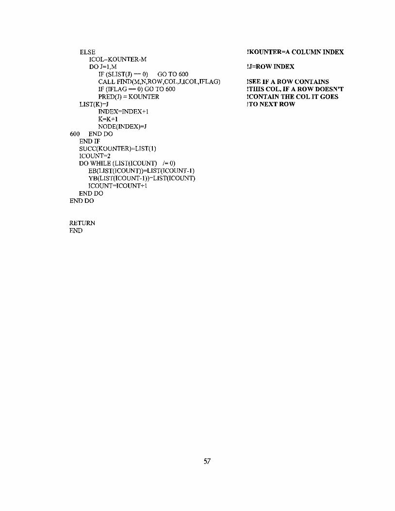
ELSE ICOL=KOUNTER-M DOJ=l,M
IF (SLIST(J) = 0) GO TO 600 CALL FIND(M,N,ROW,COL,J,ICOL,IFLAG) IF (IFLAG = 0) GO TO 600 PRED(J) = KOUNTER
LIST(K)=J INDEX=INDEX+1 K=K+1 NODE(INDEX)=J
600 ENDDO END IF SUCC(KOUNTER)=LIST( 1) ICOUNT=2 DO WHILE (LIST(ICOUNT) /= 0)
EB(LIST(ICOUNT))=LIST(ICOUNT -1) YB(LIST(ICOUNT-1))=LIST(lCOUNT) ICOUNT=ICOUNT + 1
END DO END DO
RETURN END
57
!KOUNTER=A COLUMN INDEX
!J=ROW INDEX
!SEE IF A ROW CONTAINS !TillS COL, IF A ROW DOESN'T !CONTAIN THE COL IT GOES lTONEXTROW

!************************************************************************************* ! PICKING THE NEW VARIABLE TO ENTER THE BASIS USING MODIFIED ROW FIRST !NEGATIVE METHOD. THIS METHOD FIND THE FIRST ROW WITH A NEG REDUCED !COST COEFFICIENT AND THEN SCANS THE REST OF THAT ROW FOR ANY OTHER RC !WHICH IS MORE NEGATIVE.
NBR= ROW OF VARIABLE ENTERING THE BASIS NBC= COLUMN OF VARIABLE ENTERING THE BASIS KTEST= KEEPS TRACK OF COST SO CAN COMPARE REST OF ROW
& PICK SMALLEST KSTOP= SET TO 0 WHEN ALL RC>=O
!*************************************************************************************
SUBROUTINE NEWBAS(M,N,C,NBR,NBC,KSTOP) INTEGER C(M,N) , KTEST
NBR=O NBC=O
DOI=l,M DO J=l,N
IF(C(I,J) < 0) THEN NBR=I
NBC=J KTEST=C(I,J) GO TO 40
END IF END DO
END DO
KSTOP=O GO TO 50
40 NB=NBC DO JS=NBC+l,N
JF(C(NBR,JS) < KTEST) THEN KTEST=C(NBR,JS)
NB=JS END IF
END DO
NBC=NB
50 RETURN END
!IF ALL RC ~O THEN OPTIMAL SOLUTION-EXIT
58
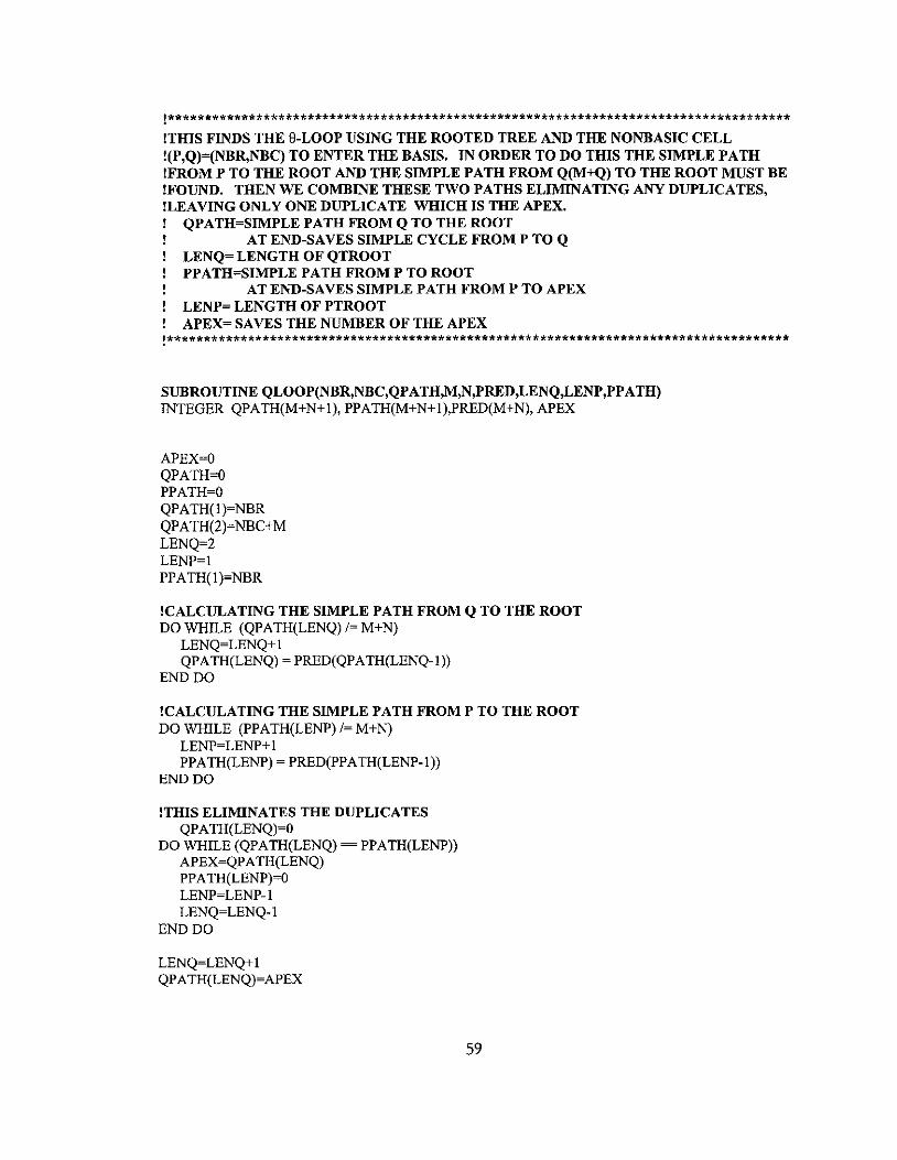
!************************************************************************************* !THIS FINDS THE 8-LOOP USING THE ROOTED TREE AND THE NONBASIC CELL !(P,Q)=(NBR,NBC) TO ENTER THE BASIS. IN ORDER TO DO THIS THE SIMPLE PATH !FROM P TO THE ROOT AND THE SIMPLE PATH FROM Q(M+Q) TO THE ROOT MUST BE !FOUND. THEN WE COMBINE THESE TWO PATHS ELIMINATING ANY DUPLICATES, !LEA VING ONLY ONE DUPLICATE WHICH IS THE APEX.
QPATH=SIMPLE PATH FROM Q TO THE ROOT AT END-SAVES SIMPLE CYCLE FROM P TO Q
LENQ= LENGTH OF QTROOT PPATH=SIMPLE PATH FROM P TO ROOT
AT END-SAVES SIMPLE PATH FROM P TO APEX LENP= LENGTH OF PTROOT APEX= SAVES THE NUMBER OF THE APEX
!*************************************************************************************
SUBROUTINE QLOOP(NBR,NBC,QPATH,M,N,PRED,LENQ,LENP,PPATH) INTEGER QPATH(M+N+l), PPATH(M+N+l),PRED(M+N), APEX
APEX=O QPATH=O PPATH=O QPATH(l)=NBR QPATH(2)=NBC+M LENQ=2 LENP=l PPATH(1 )=NBR
!CALCULATING THE SIMPLE PATH FROM Q TO THE ROOT DO WHILE (QPATH(LENQ) /= M+N)
LENQ=LENQ+ 1 QP A TH(LENQ) = PRED(QP A TH(LENQ-l»
END DO
!CALCULATING THE SIMPLE PATH FROM P TO THE ROOT DO WHILE (PPATH(LENP) /= M+N)
LENP=LENP+ 1 PP A TH(LENP) = PRED(PP A TH(LENP-l»
END DO
!THIS ELIMINATES THE DUPLICATES QP A TH(LENQ)=O
DO WHILE (QPATH(LENQ) = PPATH(LENP» APEX=QP A TH(LENQ) PP ATH(LENP)=O LENP=LENP-l LENQ=LENQ-l
END DO
LENQ=LENQ+ 1 QP ATH(LENQ)=APEX
59
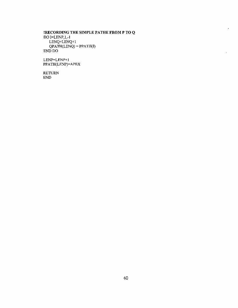
!RECORDING THE SIMPLE PATHE FROM P TO Q DO I=LENP,l,-l
LENQ=LENQ+ 1 QPATH(LENQ) = PPATH(I)
END DO
LENP=LENP+ 1 PP ATH(LENP)=APEX
RETURN END
60
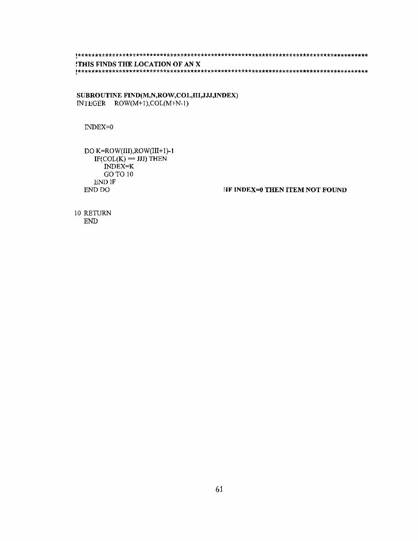
!************************************************************************************* !THIS FINDS THE LOCATION OF AN X !*************************************************************************************
SUBROUTINE FIND(M,N,ROW,COL,III,JJJ,INDEX) INTEGER ROW(M+l),COL(M+N-l)
INDEX=O
DO K=ROW(III),ROW(III+1)-1 IF(COL(K) == HI) THEN
INDEX=K GO TO 10
END IF END DO
10 RETURN END
!IF INDEX=O THEN ITEM NOT FOUND
61
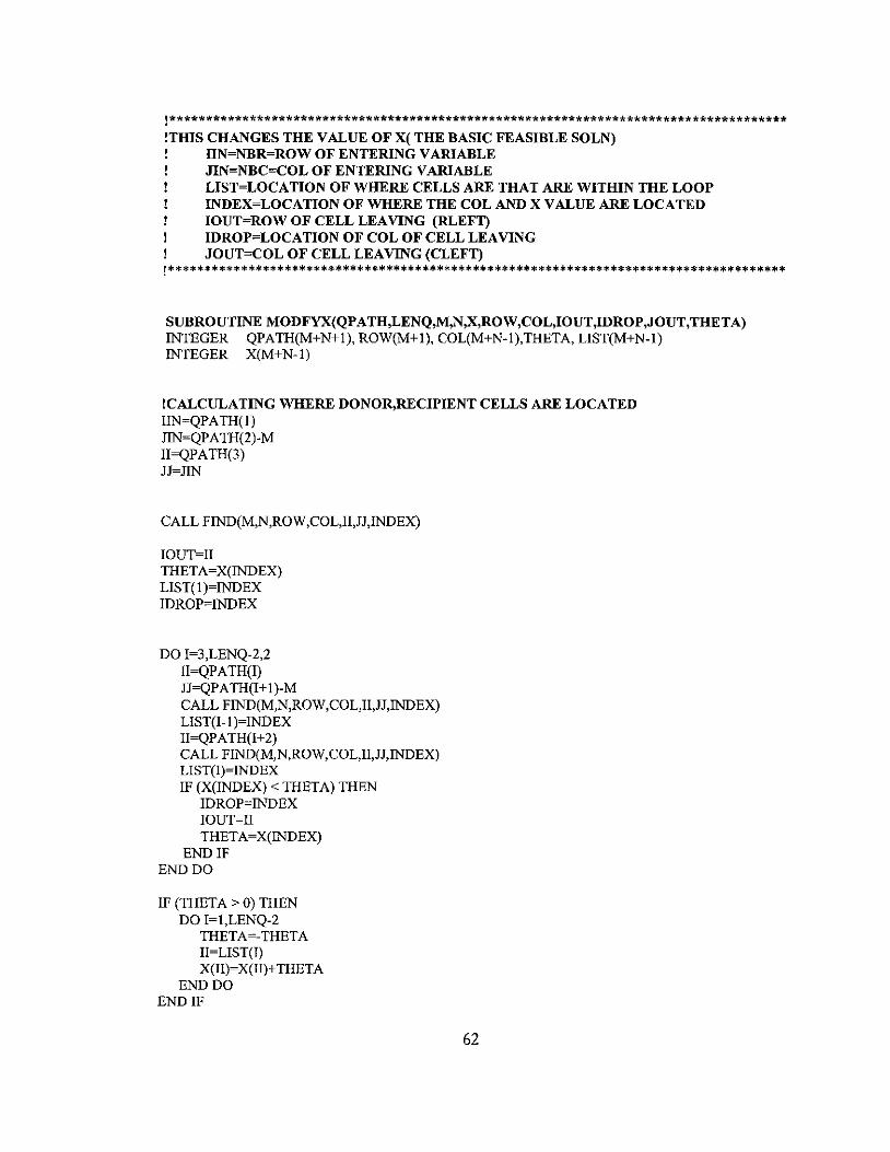
!************************************************************************************* !THIS CHANGES THE VALUE OF X( THE BASIC FEASIBLE SOLN)
IIN=NBR=ROW OF ENTERING VARIABLE JIN=NBC=COL OF ENTERING VARIABLE LIST=LOCATION OF WHERE CELLS ARE THAT ARE WITHIN THE LOOP INDEX=LOCATION OF WHERE THE COL AND X VALUE ARE LOCATED IOUT=ROW OF CELL LEAVING (RLEFT) IDROP=LOCATION OF COL OF CELL LEAVING JOUT=COL OF CELL LEAVING (CLEFT)
!*************************************************************************************
SUBROUTINE MODFYX(QPATH,LENQ,M,N,X,ROW,COL,IOUT,IDROP,JOUT,THETA) INTEGER QPATH(M+N+l), ROW(M+l), COL(M+N-l),THETA, LIST(M+N-l) INTEGER X(M+N-l)
!CALCULATING WHERE DONOR,RECIPIENT CELLS ARE LOCATED IIN=QPATH(l) JIN=QPATH(2)-M I1=QPATH(3) JJ=JIN
CALL FIND(M,N,ROW,COL,I1,JJ,INDEX)
IOUT=I1 THETA=X(INDEX) LIST(l)=INDEX IDROP=INDEX
DO I=3,LENQ-2,2 II=QPATH(I) JJ=QPATH(I+l)-M CALL FIND(M,N,ROW,COL,I1,JJ,INDEX) LIST(I-l)=INDEX II=QP A TH(I+2) CALL FIND(M,N,ROW,COL,I1,JJ,INDEX) LIST(I)=INDEX IF (X(INDEX) < THETA) THEN
IDROP=INDEX IOUT=I1 THETA=X(INDEX)
END IF END DO
IF (THETA> 0) THEN DO I=1,LENQ-2
THETA=-THETA I1=LIST(I) X(II)= X(I1)+ THETA
END DO END IF
62

THETA=-THETA JOUT=COL(IDROP)
IF (lIN> lOUT) THEN DO I=IDROP,ROW(IIN)-2
COL(I)=COL(I+ 1) X(I)= X(I + 1 )
END DO X(ROW(IIN)-l )=THETA COL(ROW(IIN)-l)=JIN DO 1=IOUT+1,IIN
ROW(I)=ROW(I)-l END DO
ELSE DO I=IDROP,ROW(IIN)+ 1,-1
COL(I)=COL(I-1 ) X(I)= X(I -1 ) END DO COL(ROW(IIN)=JIN X(ROW(IIN»=THETA DO 1=IIN+1,IOUT ROW(I)=ROW(I)+ 1 END DO
END IF
RETURN END
!NEED TO SHIFT INDICES IN COL&X TO LEFT
!NEED INDICES SIDFTED TO RIGHT IF (NBR gu.EFT) = (lIN ::; lOUT)
63
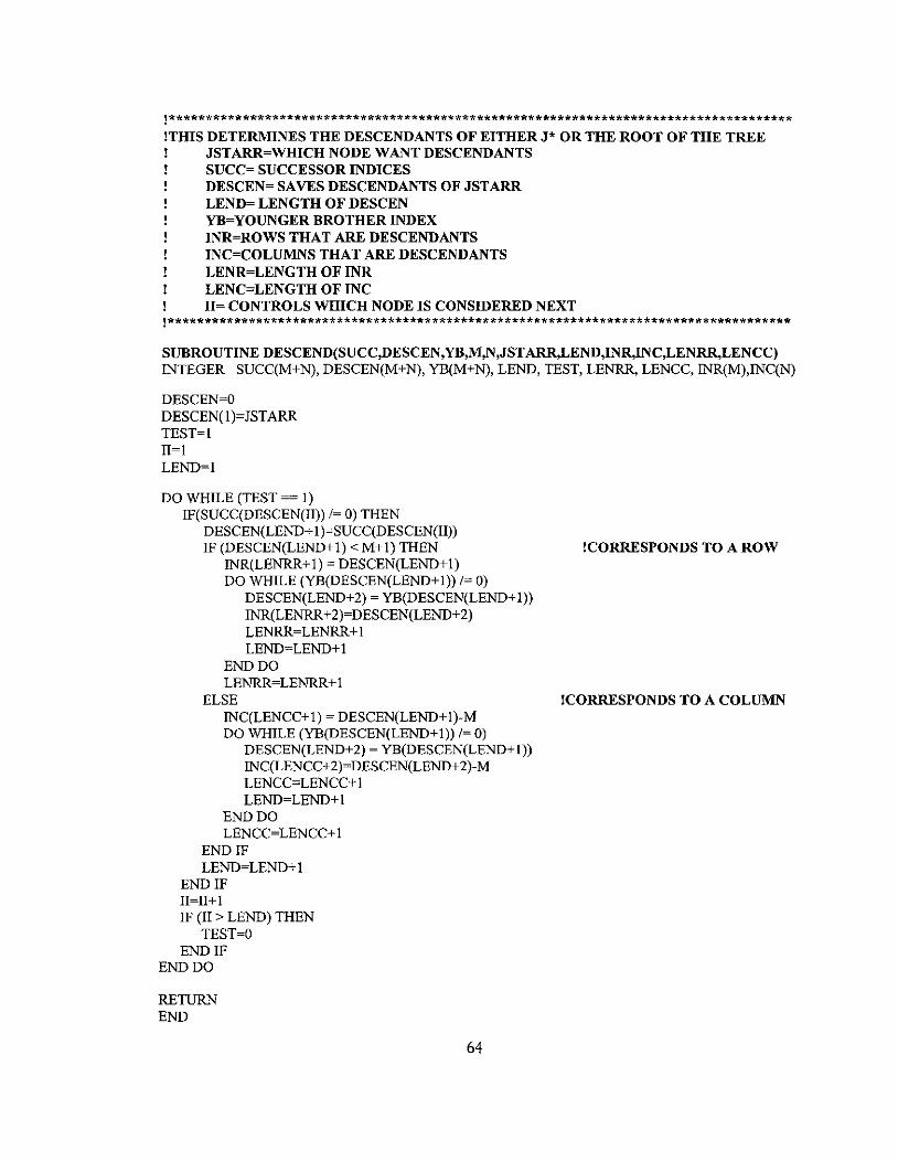
!************************************************************************************* !THIS DETERMINES THE DESCENDANTS OF EITHER J* OR THE ROOT OF THE TREE
JSTARR=WHICH NODE WANT DESCENDANTS SUCC= SUCCESSOR INDICES DESCEN= SAVES DESCENDANTS OF JSTARR LEND= LENGTH OF DESCEN YB=YOUNGER BROTHER INDEX INR=ROWS THAT ARE DESCENDANTS INC=COLUMNS THAT ARE DESCENDANTS LENR=LENGTH OF INR LENC=LENGTH OF INC 11= CONTROLS WHICH NODE IS CONSIDERED NEXT
!*************************************************************************************
SUBROUTINE DESCEND(SUCC,DESCEN,YB,M,N,JSTARR,LEND,INR,INC,LENRR,LENCC) INTEGER SUCC(M+N), DESCEN(M+N), YB(M+N), LEND, TEST, LENRR, LENCC, INR(M),INC(N)
DESCEN=O DESCEN(1)=JSTARR TEST=1 11=1 LEND=1
DO WHILE (TEST = 1) IF(SUCC(DESCEN(II» /= 0) THEN
DESCEN(LEND+ 1 )=SUCC(DESCEN(II» IF (DESCEN(LEND+1) < M+1) THEN
INR(LENRR+1) = DESCEN(LEND+1) DO WHILE (YB(DESCEN(LEND+1» /= 0)
DESCEN(LEND+2) = YB(DESCEN(LEND+ 1» INR(LENRR+2)=DESCEN(LEND+2) LENRR=LENRR+ 1 LEND=LEND+ 1
END DO LENRR=LENRR+ 1
ELSE INC(LENCC+1) = DESCEN(LEND+1)-M DO WHILE (YB(DESCEN(LEND+1» /= 0)
DESCEN(LEND+2) = YB(DESCEN(LEND+ 1» INC(LENCC+2)=DESCEN(LEND+2)-M LENCC=LENCC+ 1 LEND=LEND+ 1
END DO LENCC=LENCC+ 1
END IF LEND=LEND+ 1
END IF II=II+1 IF (II > LEND) THEN
TEST=O END IF
END DO
RETURN END
64
!CORRESPONDS TO A ROW
!CORRESPONDS TO A COLUMN
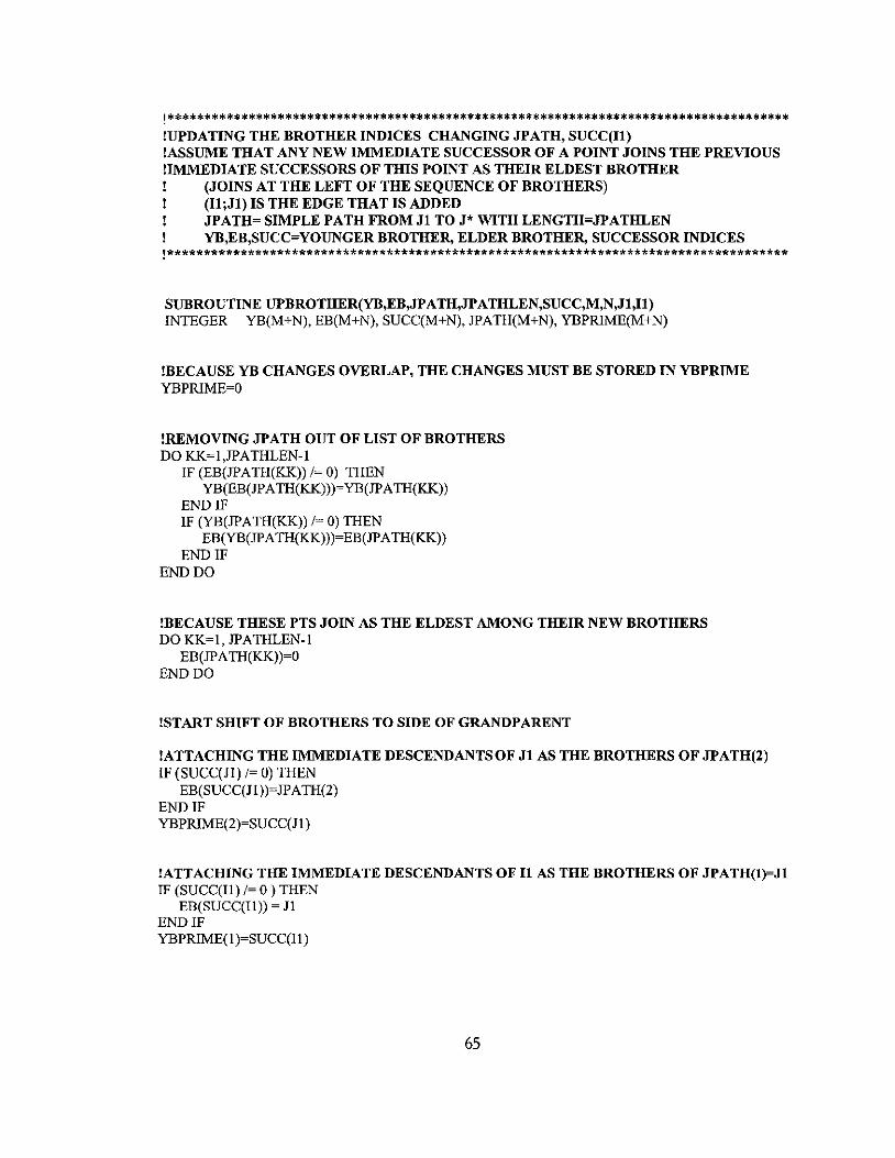
!************************************************************************************* !UPDATING THE BROTHER INDICES CHANGING JPATH, SUCC(Il) !ASSUME THAT ANY NEW IMMEDIATE SUCCESSOR OF A POINT JOINS THE PREVIOUS !IMMEDIATE SUCCESSORS OF THIS POINT AS THEIR ELDEST BROTHER
(JOINS AT THE LEFT OF THE SEQUENCE OF BROTHERS) (Il;J1) IS THE EDGE THAT IS ADDED JPATH= SIMPLE PATH FROM J1 TO J* WITH LENGTH=JPATHLEN YB,EB,SUCC=YOUNGER BROTHER, ELDER BROTHER, SUCCESSOR INDICES
!*************************************************************************************
SUBROUTINE UPBROTHER(YB,EB,JP ATH,JP ATHLEN,SUCC,M,N,J1,1l) INTEGER YB(M+N), EB(M+N), SUCC(M+N), JPATH(M+N), YBPRIME(M+N)
!BECAUSE YB CHANGES OVERLAP, THE CHANGES MUST BE STORED IN YBPRIME YBPRIME=O
!REMOVING JPATH OUT OF LIST OF BROTHERS DO KK=l,JPATHLEN-l
IF (EB(JPATH(KK» /= 0) THEN YB(EB(JPATH(KK»)=YB(JPATH(KK»
END IF IF (YB(JPATH(KK» /= 0) THEN
EB(YB(JPATH(KK»)=EB(JPATH(KK» END IF
END DO
!BECAUSE THESE PTS JOIN AS THE ELDEST AMONG THEIR NEW BROTHERS DO KK=l, JPATHLEN-l
EB(JPATH(KK»=O END DO
!START SHIFT OF BROTHERS TO SIDE OF GRANDPARENT
!ATTACHING THE IMMEDIATE DESCENDANTS OF J1 AS THE BROTHERS OF JPATH(2) IF (SUCC(J1) /= 0) THEN
EB(SUCC(J1»=JPATH(2) END IF YBPRIME(2)=SUCC(J1 )
!ATTACHING THE IMMEDIATE DESCENDANTS OF 11 AS THE BROTHERS OF JPATH(1)=J1 IF (SUCC(Il) /= 0) THEN
EB(SUCC(Il» = J1 END IF YBPRIME( 1 )=SUCC(I 1)
65
!SHIFTS JPATH AS EB OF GRANDPARENT DO KK=2,JPATHLEN-l
IF (SUCceJPATH(KK)) == JPATH(KK-l)) THEN YBPRIME(KK+l) = YB(JPATH(KK-l)) EB(YBPRIME(KK+l)) = JPATH(KK+l)
ELSE EB(SUCceJPATH(KK))) = JPATH(KK+l) YBPRIME(KK+l) = SUCceJPATH(KK))
END IF END DO
DO KK=l, JPATHLEN YB(JPATH(KK))=YBPRIME(KK)
END DO
RETURN END
66
!************************************************************************************* !THIS SUBROUTINE UPDATES THE TREE INDICES-PRED, SUCC, YB, EB USING JPATH
YB,EB,SUCC=YOUNGER BROTHER, ELDER BROTHER, SUCCESSOR INDICES (I1;Jl) IS THE EDGE THAT IS ADDED JPATH= SIMPLE PATH FROM Jl TO J* WITH LENGTH=JPATHLEN
!*************************************************************************************
SUBROUTINE UPTREE(M,N,PRED,SUCC,YB,EB,JP ATH,JPATHLEN,Jl,I1,JST AR) INTEGER PRED(M+N), SUCC(M+N), YB(M+N), EB(M+N) ,JPATH(M+N), YBIT
!UPDATING THE PREDECESSOR INDICES-ONLY ONES THAT CHANGE ARE THE JPATH !PREDECESSOR INDICES BECOME THE OPPOSITE-REVERSE OF JPATH
PRED(J1)=I1 IF (JPATHLEN > 1) THEN
DO KK =2,JP A THLEN PRED(JP A TH(KK»=JP ATH(KK-l)
END DO END IF
!UPDATING THE BROTHER INDICES- CHANGING JPATH, SUCC(Il) ! ASSUME THAT ANY NEW IMMEDIATE SUCCESSOR OF A POINT JOINS THE PREVIOUS ! IMMEDIATE SUCCESSOR OF TillS POINT AS THEIR ELDEST BROTHER !(JOINS AT THE LEFT END OF THE SEQUENCE OF BROTHERS)
YBIT=Q IF (JPATHLEN >1) THEN
YBIT=YB(JP A TH(JP A THLEN-l» END IF
CALL UPBROTHER(YB,EB,JP A TH,JP ATHLEN,SUCC,M,N,J1,Il)
!UPDATING THE SUCESSOR INDICES- ONLY CHANGE JPATH,I1,I2. SUCCESSORS !OF JPATH BECOME THEIR OLD PREDECESSOR INDEX(NEXT JPATH ENTRY) ! YBJT= OLD YB(JPATH(JPATHLEN-l» BEFORE UPDATED
SUCC(Il)=J1 IF (JPATHLEN > 1) THEN
DO KK=I,JPATHLEN-l SUCC(JPATH(KK»=JPATH(KK+l)
END DO END IF
IF (JPATHLEN > 1) THEN IF (SUCC(JSTAR) = JPATH(JPATHLEN-l» THEN
SUCC(JSTAR)=YBIT !ELSE ! SUCC(JSTAR)=SUCC(JSTAR) END IF
END IF
RETURN END
67

!************************************************************************************* !THIS SUBROUTINE UPDATES THE RELATIVE COST COEFFICIENTS
ALPHA=1 IF 11 IS A NODE CORRESPONDING TO A ROW OF THE =-1 IF OTHERWISE TRANSPORTATION ARRAY
REDCOST= REDUCED COST OF CELL ENTERING THE BASIS RINJS=THR ROW INDICES WITHIN DESJSTAR LENR= CHANGROW LENGTH CINJS=THR COL INDICES WITHIN DESJSTAR LENC= CHANGCOL LENGTH NINJR= ROW INDEX WHICH IS NOT IN DESJSTAR KKI = LENGTH OF NINJR NINJC=COLUMN INDEX WHICH IS NOT IN DESJSTAR KK2= LENGTH OF NINJC
!*************************************************************************************
SUBROUTINE UPDATE(ALPHA,M,N,REDCOST,C,RINJS,CINJS,LENR,LENC,NINJR,NINJC,KKl,KK2) INTEGER NINJC(N), NINJR(M), ALPHA, CINJS(M), RINJS(N), REDCOST, C(M,N)
!CHANGING COST COEFFICIENTS DOI=l,LENR
DOJ=1,KK2 C(RINJS(I),NINJC(J) = C(RINJS(I),NINJC(J»+ ALPHA *REDCOST
END DO END DO
DOI=l,KKl DOJ=l,LENC
C(NINJR(I),CINJS(J» = C(NINJR(I),CINJS(J» - ALPHA *REDCOST END DO
END DO
RETURN END
68
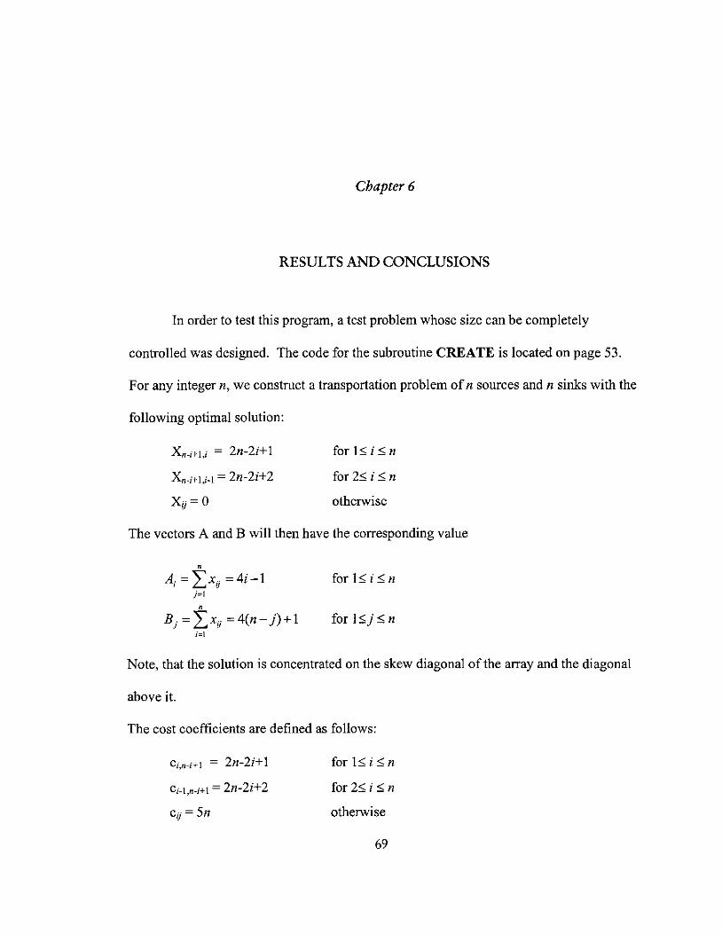
Chapter 6
RESULTS AND CONCLUSIONS
In order to test this program, a test problem whose size can be completely
controlled was designed. The code for the subroutine CREATE is located on page 53.
For any integer n, we construct a transportation problem of n sources and n sinks with the
following optimal solution:
Xn-i+l,i = 2n-2i+ 1
Xn-i+l,i-l = 2n-2i+2
Xij= 0
for 2~ i ~ n
otherwise
The vectors A and B will then have the corresponding value
n
Ai = LXii =4i-l j=1
n
B j = LXii =4(n- j)+l i=1
Note, that the solution is concentrated on the skew diagonal of the array and the diagonal
above it.
The cost coefficients are defined as follows:
Ci,n-i+l = 2n-2i+ 1
Ci-l,n-i+l = 2n-2i+2
cij = 5n
for 2~ i ~ n
otherwise
69
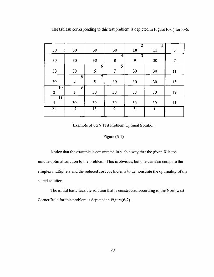
The tableau corresponding to this test problem is depicted in Figure (6-1) for n=6.
2 1 30 30 30 30 10 11 3
4 3 30 30 30 8 9 30 7
6 5 30 30 6 7 30 30 11
8 7 30 4 5 30 30 30 15
10 9 2 3 30 30 30 30 19
11 1 30 30 30 30 30 11
21 17 13 9 5 1
Example of 6 x 6 Test Problem Optimal Solution
Figure (6-1)
Notice that the example is constructed in such a way that the given X is the
unique optimal solution to the problem. This is obvious, but one can also compute the
simplex multipliers and the reduced cost coefficients to demonstrate the optimality ofthe
stated solution.
The initial basic feasible solution that is constructed according to the Northwest
Comer Rule for this problem is depicted in Figure(6-2).
70

3 30 30 30 30 10 11 3
7 30 30 30 8 9 30 7
11 0 30 30 6 7 30 30 11
15 30 4 5 30 30 30 15
2 13 4 2 3 30 30 30 30 19
5 5 1 1 30 30 30 30 30 11
21 17 13 9 5 1
6 x 6 Test Problem Initial Basic Feasible Solution-NW Comer Rule
Figure (6-2)
Notice that the Northwest Comer Rule will produce a solution where the basic
cells form a staircase, starting at the northwest comer of the array and ending at the
bottom right hand comer. It is clear the initial basic feasible solution provided by the
Northwest Comer Rule is among the most expensive basic feasible solutions of the test
problem.
Thus, we start with the most expensive solution of the problem and generate the
least expensive solution. As expected, the test problem turned out to be an excellent one
for testing the program.
Figure (6-3) contains the results of four runs of the test problem, corresponding to
n=100,300,500, and 1000.
71
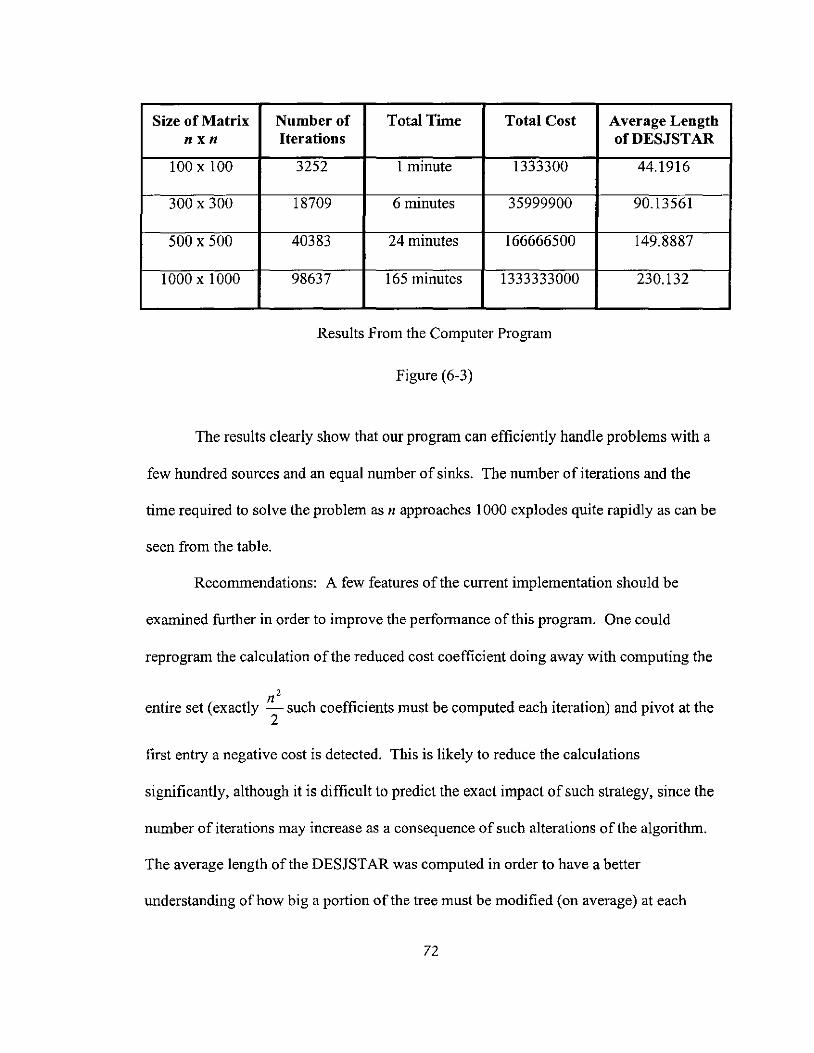
Size of Matrix Number of Total Time Total Cost Average Length nxn Iterations ofDESJSTAR
100 x 100 3252 1 minute 1333300 44.1916
300 x 300 18709 6 minutes 35999900 90.13561
500 x 500 40383 24 minutes 166666500 149.8887
1000 x 1000 98637 165 minutes 1333333000 230.132
Results From the Computer Program
Figure (6-3)
The results clearly show that our program can efficiently handle problems with a
few hundred sources and an equal number of sinks. The number of iterations and the
time required to solve the problem as n approaches 1000 explodes quite rapidly as can be
seen from the table.
Recommendations: A few features of the current implementation should be
examined further in order to improve the performance of this program. One could
reprogram the calculation of the reduced cost coefficient doing away with computing the
2
entire set (exactly ~ such coefficients must be computed each iteration) and pivot at the 2
first entry a negative cost is detected. This is likely to reduce the calculations
significantly, although it is difficult to predict the exact impact of such strategy, since the
number of iterations may increase as a consequence of such alterations of the algorithm.
The average length of the DESJST AR was computed in order to have a better
understanding of how big a portion of the tree must be modified (on average) at each
72

step. This gave us some understanding of how complex the tree structure is for the
current test problem. The average length ofDESJSTAR was found to be relatively small
compared to the size of the test problem (2n nodes). More difficult test problems, where
there are far more (10 to 100 times) sinks than sources, can be easily developed along the
same lines of this test problem. The corresponding trees will have a more complex
structure because they will have much more lateral width than the trees of the test
problem used in this paper. Therefore, this new test problem would further test the
efficiency of the subroutines within this program that are concerned with the tree design.
73
BIBLIOGRAPHY
Glover, Fred, et aL "A Computation Study on Start Procedures, Basis Change Criteria, and Solution Algorithms for Transportation Problems." Management Science. Volume 20, Number 5. January 1974: 793-812.
Gould, Ronald. Graph Theory. Menlo Park, California: Benjamin/Cummings Publishing Co., Inc., 1988.
Luenberger, David G. Linear and NonLinear Programming. 2nd ed. Reading, Massachusetts: Addison-Wesley Publishing Co., 1984.
Murty, Katta G. Linear Programming. Upper Saddle River, New Jersey: Prentice Hall, 1995.
Murty, Katta G. Network Programming. Englewood Cliffs, New Jersey: Prentice Hall, 1992.
Murty, Katta G. Operations Research: Deterministic Optimization Models. Upper Saddle River, New Jersey: Prentice Hall, 1995.
Taha, Hardy A. Operations Research: An Introduction. 5th ed. New York: Macmillan Publishing Co., 1992.
74

VITA
Name of Author: Alissa Michele (Andreichuk) Sustarsic
Place of Birth: Date of Birth:
EDUCATION: • MS in Mathematical Science May 1999
University of North Florida • BS in Mathematics with Minor in Biology May 1997
Jacksonville University Summa Cum Laude with Departmental Honors in Mathematics
TEACHING EXPERIENCE: • University of North Florida, Mathematics and Statistics Department
Instructor in College Algebra, Graduate Teaching Assistant • University of North Florida, Quest Program, Center of Multicultural Affairs
Mathematics Instructor Duties- Planning & Teaching Skills for the Clast Exam
ACHIEVEMENTS: • UNF Outstanding Graduate Student of the Year 1999 • JU Fred E. Noble Gold Medal for Scholarship-Highest Academic Award at Graduation • JU College of Arts and Sciences 1996-1997 Outstanding Student • JU Division of Science and Mathematics Student of the Year 1997 • JU Outstanding Mathematics Student of the Year 1996 & 1997 • George Washington University Summer Program for Women In Mathematics 1996
Chosen as 1116 College Senior Women, a 1 Month of Mathematics Intensive Study • Florida Academic Scholar, JU Trustees Scholarship, Robert C. Byrd Scholarship(JU)
PROFESSIONAL ORGANIZATIONS: • Pi Mu Epsilon National Mathematics Honor Society: President-UNF • Phi Kappa Phi National Honor Society • Green Key Honorary Leadership Society • Alpha Delta Pi Sorority • Omicron Delta Kappa National Leadership Honor Society
SPORTS AT JACKSONVILLE UNIVERSITY • Women's Varsity Soccer: Charter Member, Captain, Scholarship Recipient,
GTE Academic All District III Team, Sun Belt Conference Academic Team 1996 Women's Club Soccer: Charter Member, President/Treasurer
75