An efficient meta-heuristic algorithm for grid computing

1 23

Journal of CombinatorialOptimization ISSN 1382-6905 J Comb OptimDOI 10.1007/s10878-013-9644-6

An efficient meta-heuristic algorithm forgrid computing

Zahra Pooranian, Mohammad Shojafar,Jemal H. Abawajy & Ajith Abraham

1 23

Your article is protected by copyright and all

rights are held exclusively by Springer Science

+Business Media New York. This e-offprint is

for personal use only and shall not be self-

archived in electronic repositories. If you wish

to self-archive your article, please use the

accepted manuscript version for posting on

your own website. You may further deposit

the accepted manuscript version in any

repository, provided it is only made publicly

available 12 months after official publication

or later and provided acknowledgement is

given to the original source of publication

and a link is inserted to the published article

on Springer's website. The link must be

accompanied by the following text: "The final

publication is available at link.springer.com”.

J Comb OptimDOI 10.1007/s10878-013-9644-6

An efficient meta-heuristic algorithm for gridcomputing

Zahra Pooranian · Mohammad Shojafar ·Jemal H. Abawajy · Ajith Abraham

© Springer Science+Business Media New York 2013

Abstract A grid computing system consists of a group of programs and resources thatare spread across machines in the grid. A grid system has a dynamic environment anddecentralized distributed resources, so it is important to provide efficient schedulingfor applications. Task scheduling is an NP-hard problem and deterministic algorithmsare inadequate and heuristic algorithms such as particle swarm optimization (PSO) areneeded to solve the problem. PSO is a simple parallel algorithm that can be appliedin different ways to resolve optimization problems. PSO searches the problem spaceglobally and needs to be combined with other methods to search locally as well. Inthis paper, we propose a hybrid-scheduling algorithm to solve the independent task-scheduling problem in grid computing. We have combined PSO with the gravitationalemulation local search (GELS) algorithm to form a new method, PSO–GELS. Ourexperimental results demonstrate the effectiveness of PSO–GELS compared to otheralgorithms.

Keywords Grid computing · PSO algorithm · GELS · Scheduling ·Independent tasks

Z. PooranianGraduate School, Dezful Islamic Azad University, Dezful, Iran

M. Shojafar (B)Department of Information Engineering, Electronics and Telecommunications (DIET),Sapienza University of Rome, Via Eudossiana 18, 00184 Rome, Italye-mail: [email protected]

J. H. AbawajySchool of Information Technology, Deakin University, Waurn Ponds, VIC, Australia

A. AbrahamMachine Intelligence Research Labs (MIR Labs), Scientific Network for Innovationand Research Excellence, P.O. Box 2259, Auburn, WA 98071-2259, USA

123

Author's personal copy

J Comb Optim

1 Introduction

Grid computing was introduced in the early 1990s by a supercomputing committeewhose goal of using computing resources in a convenient form for calculations wascomplicated by the fact that the resources were distributed geographically. Grid com-puting enables controlling a wide range of heterogeneous, distributed resources to exe-cute computations and data-intensive applications (Garg et al. 2010). The basic idea ofgrid computing is that participating machines share resources through a transparent andreliable software layer. The software layer is responsible for resource virtualization,resource discovery and search, and managing running applications. Two organizationsthat are working on developing large-scale data collections are the European data gridand Globus. Systems in a service grid provide services that cannot be provided witha single machine (Sullivan et al. 1997; Foster et al. 2002). The first phase of grid taskscheduling is resource discovery, which generates a list of potential resources. Thesecond phase includes gathering information about these resources and choosing thebest set of resources matching the application’s requirements. In the third phase, thetask is executed, which involves file staging and cleanup (Yan-ping et al. 2008).

Grid resources are shared as distributed and heterogeneous resources that belong toorganizations that have their own policies. Scheduling algorithms must therefore beconsistent with changes in workloads and available resources to achieve acceptableperformance and also to comply with time limits. The grid resource broker, which isresponsible for scheduling applications for users, should be an efficient schedulingalgorithm. Task scheduling is an NP-hard problem, and scheduling algorithms can becategorized into deterministic algorithms and approximate algorithms. Deterministicalgorithms are able to find exactly the optimal result, but they cannot solve NP-hardoptimization problems quickly, as their time to arrive at a solution increases exponen-tially. Approximate algorithms can find good (near optimal) solutions for optimizationproblems in a short time. Approximate algorithms can be categorized into heuristic andmeta-heuristic algorithms. There are several measures for categorizing meta-heuristicalgorithms, such as whether they are based on a single solution or on a population.Single-solution-based algorithms, such as simulated annealing (SA), tabu search (TS),and gravitational emulation local search (GELS), modify a single solution during thesearch process. In contrast, population-based algorithms, such as partial swarm opti-mization (PSO), genetic algorithms (GAs), and ant colony optimization, consider apopulation of solutions. In addition, some algorithms search the problem space glob-ally, while others search it locally.

Most of these algorithms try to minimize makespan. Many meta-heuristic algo-rithms have been proposed for task scheduling in a grid environment, including GAs(Gao et al. 2005), SA (Orosz and Jacobson 2002), TS (Benedict and Vasudevan 2008),two-phase encoding particle swarm optimization (Shiau and Huang 2012; Shiau 2011),and PSO (Zhang et al. 2008). Hybrid meta-heuristic algorithms, in which one algo-rithm is used as the main algorithm and others are used to improve the solutions, arealso being closely studied. These include the combinations GA–SA (Cruz-Chavez etal. 2010), GA–TS (Xhafa et al. 2009), GA–GELS (Pooranian et al. 2011, 2013b),PSO–SA (Chen et al. 2009), Queen Bee (Pooranian et al. 2012), HSPN (Shojafaret al. 2013, 2010), GLOA (Pooranian et al. 2013a), and PSO–TS (Padmavathi and

123


J Comb Optim

Mercy shalinie 2010). PSO has the better ability for global searching and has beensuccessfully applied in many areas. It also has fewer parameters than either GAs orSA. Furthermore, PSO works well for most global optimization problems. But PSO’slocal search ability is weak, and there is a high probability of becoming trapped in alocal optimum. In this paper, we combine PSO with GELS, a local search algorithmthat improves PSO’s performance in finding a solution. The proposed hybrid algorithm(PSO–GELS) decreases makespan and minimizes the number of tasks that miss theirdeadlines.

The rest of this paper is organized as follows. Section 2 summarizes previous relatedwork in this field. Section 3 describes our computing system model. Sections 4 to 7describe the intelligent PSO and GELS algorithms, and Sect. 8 describes our proposedalgorithm in detail. Section 9 compares our proposed algorithm with several similaralgorithms, and the final section presents our conclusion and future research directions.

2 Related work

A combined optimization algorithm using PSO and SA was proposed in Weijun et al.(2004) for the task scheduling problem. A particle consists of m segments and everysegment has n different job numbers, representing the processing orders of n jobs onm machines. Thus, we have m machines and n jobs, which convert the continuousoptimization problem to a discrete optimization problem. The real optimum valuesare rounded to the nearest integers. In this algorithm, the PSO results are given to theSA algorithm to avoid being trapped in a local minimum.

In Sivanandam and Visalakshi (2007), a combination of PSO and SA was proposedfor scheduling independent tasks with a dynamically varying inertia to provide abalance between the global and local explorations. The algorithm requires less iterationthan PSO on the average to find a sufficiently optimal solution. Hence, our proposedmethod also combines compatible AI algorithms to increase the speed of grid taskscheduling.

The discrete PSO algorithm was proposed in Izakian et al. (2009) for task schedulingin grid systems. The scheduler aims to simultaneously minimize makespan and flowtime. This algorithm uses a matrix in which each column represents a job’s resourceallocations and each row represents jobs allocated to a resource. This inspired us toillustrate our proposed method with a 2D matrix.

The method in Zhang et al. (2008) solves the task scheduling problem by usingthe PSO algorithm with the small position value (SPV) rule borrowed from randomkey representation. The SPV rule can convert continuous position values to discretepermutations in the PSO algorithm. Each particle represents a potential solution to theresource scheduling problem. Simulation results demonstrate that the PSO algorithmcan perform better than GAs for large scale optimization problems. We will similarlydemonstrate that our proposed hybrid method performs better than GAs.

In Mathiyalagan et al. (2010), a list scheduling algorithm is presented that usesPSO based on a TS, combining the advantages of both algorithms. It also uses aswap operation to create a new particle. Because we need fast convergence in a gridscheduling problem, and the inertia weight is the deciding factor for the convergence

123


J Comb Optim

speed of the PSO algorithm, the algorithm in Mathiyalagan et al. (2010) modifiesthe inertia equation. This increases the speed of convergence, boosts efficiency, andachieves better results. In this paper we also improved PSO by modifying the inertiaparameter, and our algorithm achieves better performance than other methods andoptimizes the results.

In Tao et al. (2011), the rotary chaotic PSO algorithm is presented for workflowscheduling in grid computing. A new method called the rotary discrete rule is proposedfor changing a continuous space to a discrete space. The method avoids local optimain perturbations of the chaotic sequence, and it makes better modifications of particlesthan other methods such as Gauss or Cauchy. Our method also pays close attention toseveral quality of service (QOS) parameters such as availability, reliability, cost, andtime concurrency. In our hybrid method, we use chaotic activity to schedule tasks.

In Liu et al. (2010), fuzzy matrices are used for the position and velocity matrix inPSO instead of real vectors. This method is shown to be better than SA and GAs in itsspeed of convergence and its ability to find optimal solutions. The paper dynamicallygenerates an optimal schedule, completing the tasks within a minimal period of time aswell as utilizing the resources efficiently. In our proposed method, we use an optimalscheduler with various parameters that will be discussed below.

In Yusof et al. (2010), the TS algorithm, which is a local search algorithm, is usedfor scheduling tasks in a grid system. The TS algorithm uses a perturbation schemefor pair changing.

In Joshua Samuel Raj and Vasudevan (2011), the SA algorithm is used to solve theworkflow scheduling problem in a computational grid. Simulation results show thatthis algorithm is highly efficient in a grid environment.

In Barzegar et al. (2009), the GELS algorithm was used for resource reservation andscheduling. Here, if one resource is unable to execute a task within its designated dead-line, the objective function switches resources and allocates the task to other resourcesfor execution. Our proposed method uses the GELS algorithm in combination withPSO to improve some QOS parameters in grid scheduling.

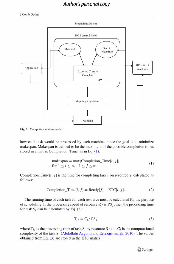
3 Computing system model

Before presenting our proposed algorithm, we describe the computing system model onwhich the algorithm is based and assessed. Grid models are composed of a number ofhomogeneous machines that are used to run applications. Figure 1 shows an overviewof the grid model. The scheduler system consists of a scheduler, an application model,and a set of computing machines. For the application model and homogeneous groupof machines, an estimate of the expected time for each task to execute on each machineis known beforehand, and it is assumed that these values are available to the scheduler(Maheswaran 1999). The values have been stored in an m ×n matrix ETC, where m isthe number of machines and n is the number of tasks. Obviously, n/m will generallybe greater than 1, with more tasks than machines, so that certain machines will need tobe assigned multiple tasks. Each column j of the ETC matrix contains estimates of theexpected running times of each task i on machine j . In addition, a 1 ×m matrix Readystores the time that each machine requires to complete its current task. We consider

123


J Comb Optim

Meta task Set of Machines

Expected Time to Complete

Mapping Algorithm

ApplicationHC suite of machines

Mapping

HC System Model

Scheduling System

Fig. 1 Computing system model

how each task would be processed by each machine, since the goal is to minimizemakespan. Makespan is defined to be the maximum of the possible completion timesstored in a matrix Completion_Time, as in Eq. (1):

makespan = max(Completion_Time[i, j])for 1 ≤ i ≤ n, 1 ≤ j ≤ m

(1)

Completion_Time[i, j] is the time for completing task i on resource j , calculated asfollows:

Completion_Time[i, j] = Ready[ j] + ETC[i, j]. (2)

The running time of each task for each resource must be calculated for the purposeof scheduling. If the processing speed of resource R j is PS j , then the processing timefor task Si can be calculated by Eq. (3):

Ti j = Ci/ PS j (3)

where Ti j is the processing time of task Si by resource R j and Ci is the computationalcomplexity of the task Si (Abdollahi Azgomi and Eetezari-maleki 2010). The valuesobtained from Eq. (3) are stored in the ETC matrix.

123


J Comb Optim

The purpose of grid scheduling is that tasks should be allocated to resources in sucha way that makespan and the numbers of tasks that miss their deadlines are minimized.

4 The PSO algorithm

The PSO algorithm, which was proposed in Eberhat and Kennedy (1995), is a sto-chastic optimization technique (Shi and Eberhat 1998) that operates on the principleof social behavior behind bird flocking and fish schooling (Shi and Eberhat 1999). Forexample, birds migrate to find food, and they begin by flying behind birds that havemore experience and others then fly behind them; thus, birds use the experience ofother birds in their orderly flying. Something that is interesting about the migrationof birds is that if a bird feels it has more experience than the bird in front of it, theyexchange positions so that the bird that has more experience moves to the forwardposition. In this way, the birds all use their experience to move to the correct place intheir migration. The same situation occurs in schools of fish, and the idea used in thePSO optimization technique is taken from such behavior. It can be said that the swarmreaction has the ability to solve optimization problems.

In a PSO system, a swarm of individuals (called particles) fly through the searchspace. Each particle represents a candidate solution to the optimization problem. Theposition of a particle is influenced by the best position (pbest) it has visited, i.e., by itsown experience and the experience of neighboring particles. When the neighborhoodof a particle is the entire swarm, the best position in the neighborhood is referred to asthe global best position of the particle, and the resulting algorithm is known as gbest.PSO has the following parameters:

Vmax maximum particle velocity;ω Inertia weight factor;

Rand1 and Rand2 random numbers with a uniform distribution on the interval [0, 1];C1 and C2 positive constants, respectively called the cognitive and the social

parameters.

When all particles have been initialized, an iterative optimization process beginsin which the positions and velocities of all particles are revised through the recursiveequations (4) and (5):

Vi+1 = ω Vi + C1rand1(pbesti − Xi

) + C2rand2(gbesti − Xi

)(4)

Xi+1 = Xi + Vi+1 (5)

where Xi and Vi are the position and velocity of the i th particle. Here, the particleflies through potential solutions toward pbesti and gbesti in a navigated way, whilestill exploring new areas by the stochastic mechanism to escape from local optima.The inertia weight can be dynamically varied by applying an annealing scheme forthe ω-setting of the PSO, where ω decreases from ω = 0.9 to ω = 0.1[20] over the

123


J Comb Optim

entire run. In general the inertia weight ω is set according to Eq. (6):

ω = ωmax − ωmax − ωmin

i termax× i ter (6)

where ωmax is the initial value of the weighting coefficient, ωmin is the final value ofthe weighting coefficient, i termax is the maximum number of iterations, and iter is thecurrent iteration.

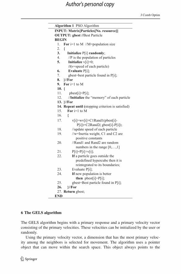
Performance is significantly improved by varying the inertia.Pseudocode for the PSO algorithm (Cruz et al. 2003) is shown below in Algorithm 1.

As can be seen, the initial positions and velocity of particles in the search area aredetermined randomly. Then the fitness function is calculated for all particles. Next, thefitness of all of the particles is compared, and if the fitness of any particle is less thanthe fitness of the related pbest particle that particles’ coordinate is stored in pbest. Thengbest is set to the best pbest value. The new coordinates of the particles are obtainedwith (4) and (5). These steps are repeated for the maximum number of iterations.

5 The GELS algorithm: background

Voudouris and Tsang (1995) proposed the guided local search algorithm for searching asearch space with an NP-hard solution. Webster (2004) proposed a powerful algorithmthat he called the GELS algorithm. This algorithm mimicks gravitational attraction tosearch within a search space. Each response (problem solution) has different neighbors,which can be grouped based on problem-specific criteria. A dimension consists of theneighbors in a neighbor group. A primary velocity is defined for each dimension. Adimension that has greater primary velocity has a more apparent response (solution)for the problem. The GELS algorithm uses two methods to calculate gravitational forcebetween the responses in a search space. The first method selects a response from thelocal neighbor space of the current response, and gravitational force is calculated for thetwo responses. The second method calculates gravitation force for all of the neighborresponses in a neighbor space of the current response rather than a single response. TheGELS algorithm also uses two methods to implement movement in the search space.The first method allows movement from the current response toward the response tothe current response in local neighbor spaces. The second method allows movementtoward the responses outside of the current response’s local neighbor spaces in additionto the neighboring responses. Each of these movement methods can be combined witheach of the gravitational force methods; as a result, there are four models for the GELSalgorithm.

Balachandar and Kannan (2007) used GELS to solve the traveling salesman problemand compared it with other algorithms such as hill climbing and SA. The results showedthat when the size of a problem is small, all of the algorithms perform equally well,but when the size of a problem is large, GELS obtains better results than the otheralgorithms.

123


J Comb Optim

6 The GELS algorithm

The GELS algorithm begins with a primary response and a primary velocity vectorconsisting of the primary velocities. These velocities can be initialized by the user orrandomly.

Using the primary velocity vector, a dimension that has the most primary veloc-ity among the neighbors is selected for movement. The algorithm uses a pointerobject that can move within the search space. This object always points to the

123


J Comb Optim

response with the greatest weight. For the first method, each iteration of the algo-rithm begins by selecting a dimension for obtaining a neighbor response to thecurrent response, and a candidate response is selected from this dimension. Thegravitational force of the current and candidate responses are calculated and thenadded to the primary velocity of the dimension that was used to obtain the can-didate response; this is referred to as updating the primary velocity. In the nextiteration, the primary velocity vector is checked and used to select the new move-ment direction for continuing the response search. For the second method, eachiteration of the algorithm is similar to the iterations of the first method exceptthat instead of considering gravitational force and updating the primary velocityvector for a single candidate response in the current dimension, the gravitationalforce of each candidate response in the current dimension is considered and theprimary velocity for each candidate response in the current dimension is updated.This algorithm calculates the gravitational force f between two responses usingEq. (7):

f = G(CU − CA)

R2 (7)

where CA and CU are the candidate response and current response, respectively, G is aconstant with the value 6.672, and R is the neighbor radius between the two responsesin the search space. The value R can be constant or changed intelligently during anyiteration. The algorithm terminates when one of the following occurs: either the pri-mary velocity for all equal response dimensions (all elements of the primary velocityvector) is zero, or the maximum number of algorithm iterations has been reached(Webster 2004).

Another parameter used in this algorithm is the maximum primary velocity, which isthe maximum value that elements of the primary velocity vector can have. The primaryvelocity parameter that selects the motion direction is used to obtain a neighbor, and thisparameter can prevent increasing the motion of the primary velocity vector elements.Algorithm 2 presents the GELS pseudocode:

7 The PSO algorithm for solving the task scheduling problem

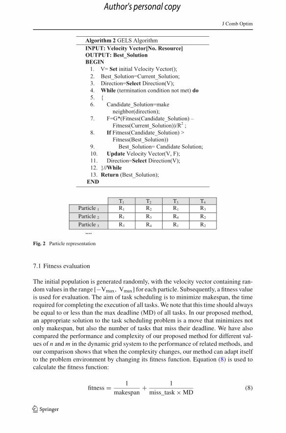
One of the key issues in successfully applying PSO to job scheduling con-cerns deciding how to encode a schedule as a search solution, i.e., findinga suitable mapping between problem solutions and PSO particles. In our pro-posed method, each particle represents a feasible solution for task assignmentusing a vector of n elements, where each element is a randomly produced inte-ger value between 1 and m. Figure 2 illustrates the allocation of four tasksto four resources. For example, in Particle 1, tasks T1 and T3 are assigned toresource R1 and tasks T2 and T4 are assigned to resource R2 and R3, respec-tively.

123


J Comb Optim

T1 T2 T3 T4

Particle 1 R1 R2 R1 R3



....

Fig. 2 Particle representation

7.1 Fitness evaluation

The initial population is generated randomly, with the velocity vector containing ran-dom values in the range [−Vmax, Vmax] for each particle. Subsequently, a fitness valueis used for evaluation. The aim of task scheduling is to minimize makespan, the timerequired for completing the execution of all tasks. We note that this time should alwaysbe equal to or less than the max deadline (MD) of all tasks. In our proposed method,an appropriate solution to the task scheduling problem is a move that minimizes notonly makespan, but also the number of tasks that miss their deadline. We have alsocompared the performance and complexity of our proposed method for different val-ues of n and m in the dynamic grid system to the performance of related methods, andour comparison shows that when the complexity changes, our method can adapt itselfto the problem environment by changing its fitness function. Equation (8) is used tocalculate the fitness function:

fitness = 1

makespan+ 1

miss_task × MD(8)

123


J Comb Optim

where miss_task is the number of tasks that miss their deadlines in the solution, andMD is the maximum deadline for all tasks.

7.2 Particle modification

Particles’ velocities and positions are updated using Eqs. (4) and (5). After generat-ing a new population, real values such as 2.25 may have been generated as particlepositions. These values are invalid for indicating the number of resources. Therefore,the algorithm rounds the real values to the nearest integers. In this way, a continu-ous optimization problem is converted to a discrete optimization problem. Our hybridalgorithm uses Eq. (6) to calculate ω in each iteration of the algorithm. Selection ofthe correct inertia weights will greatly impact the algorithm’s performance so that itavoids falling into a local minimum.

7.3 Force calculation

The gravitational force between the current and candidate particles is calculated usingEq. (9):

force = G × fitness (candidate_particle) − fitness (current_particle)

R2 (9)

8 The PSO–GELS algorithm

The PSO algorithm uses different search points, and these points are close to theoptimum point with their pbest and gbest values. PSO can be used for continuous anddiscrete problems, and it is good for global searches in the problem space. But it isweak for local searches, with a significant probability of becoming trapped in a localoptimum in the last iteration. PSO converges globally because it searches globally. Italways tries to move to solutions that have better fitness functions in a purely stochasticsearch problem space. It does not pay close attention to local subspaces so it is unableto recognize and avoid local optima. As a result, PSO may become trapped in localoptima and have a low convergence rate in the late iterative process. One option foraddressing this problem is to use local search algorithms such as GELS or SA thatcan avoid local optima. SA is much slower than GELS when combined with PSO,so we have chosen to use GELS. Although GELS behaves like a greedy algorithm, itdoes not always move to better fitness functions. It tests available solutions to find thebest solution and does not try to search the problem space purely stochastically.

Our proposed scheduling algorithm uses PSO as the main search algorithm, whileGELS is used to improve the population. There are two reasons for using both algo-rithms. First, we need an algorithm that is based on a population that can search theentire grid space for this problem. Second, the grid environment is dynamic, so thescheduling algorithm must be fast enough to adapt with the natural grid environmentand must be able to converge faster than other algorithms. Moreover, although PSO isweak for local searches, our combination of PSO with an algorithm that is strong in

123


J Comb Optim

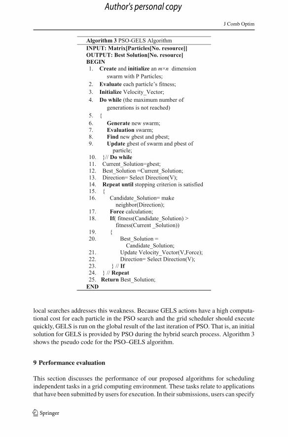
local searches addresses this weakness. Because GELS actions have a high computa-tional cost for each particle in the PSO search and the grid scheduler should executequickly, GELS is run on the global result of the last iteration of PSO. That is, an initialsolution for GELS is provided by PSO during the hybrid search process. Algorithm 3shows the pseudo code for the PSO–GELS algorithm.

9 Performance evaluation

This section discusses the performance of our proposed algorithms for schedulingindependent tasks in a grid computing environment. These tasks relate to applicationsthat have been submitted by users for execution. In their submissions, users can specify

123


J Comb Optim

Table 1 PSO algorithmparameters

Parameter Value

Vmax Number of resources

C1, C2 1.49

Initial velocity [1, Wmax]ωmax 0.9

ωmin 0.1

Table 2 GELS algorithmparameters

Parameter Value

Initial velocity [1, Wmax]Wmax Number of tasks

R 1

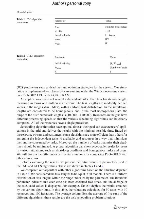
QOS parameters such as deadlines and optimum strategies for the system. Our simu-lation is implemented with Java software running under the Win XP operating systemon a 2.66 GHZ CPU with 4 GB of RAM.

An application consists of several independent tasks. Each task has its own length,measured in terms of a million instructions. The task lengths are randomly definedvalues in the range (Min…Max), with a uniform task distribution. In the simulation,lengths are considered to be homogenous, and in the most homogenous state, therange of the distributed task lengths is (10,000…110,000). Resources in the grid havedifferent processing speeds so that the various scheduling algorithms can be clearlycompared. All of the resources have a single processor.

Scheduling algorithms that have optimal time as their goal can execute users’ appli-cations in the grid and deliver the results with the minimal possible time. Based onthe resource owners and customers, some algorithms are more efficient than others forassigning the independent tasks to available grid resources in a way that minimizesthe runtime consumed by tasks. Moreover, the numbers of tasks that miss their dead-lines should be minimized. A proper algorithm can show acceptable results for usersin various situations, such as short/long deadlines and homogenous tasks and users.We will discuss the different experimental situations for comparing PSO–GELS withother algorithms.

Before examining the results, we present the initial values of parameters used inthe PSO and GELS algorithms. These are shown in Tables 1 and 2.

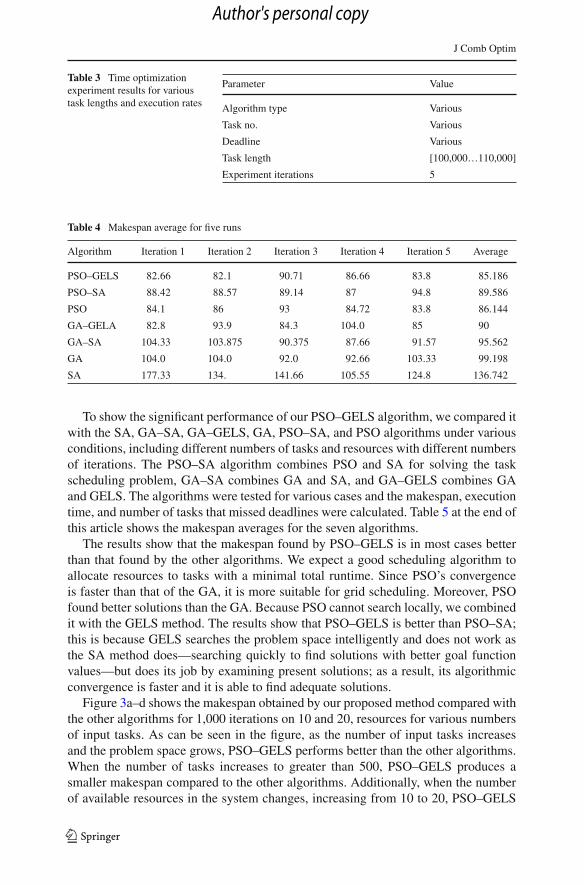
We compared our algorithm with other algorithms based on the situation depictedin Table 3. We considered the task lengths to be equal in all models. There is a uniformdistribution of task lengths within the range indicated by the parameter. The iterationsparameter indicates that each case has been executed five times, and the average ofthe calculated values is displayed. For example, Table 4 depicts the results obtainedby the various algorithms. In this table, the values are calculated for 50 tasks with 10resources and 100 iterations. The average column lists the average of five runs of thedifferent algorithms; these results are the task scheduling problem solutions.

123


J Comb Optim

Table 3 Time optimizationexperiment results for varioustask lengths and execution rates

Parameter Value

Algorithm type Various

Task no. Various

Deadline Various

Task length [100,000…110,000]

Experiment iterations 5

Table 4 Makespan average for five runs

Algorithm Iteration 1 Iteration 2 Iteration 3 Iteration 4 Iteration 5 Average

PSO–GELS 82.66 82.1 90.71 86.66 83.8 85.186

PSO–SA 88.42 88.57 89.14 87 94.8 89.586

PSO 84.1 86 93 84.72 83.8 86.144

GA–GELA 82.8 93.9 84.3 104.0 85 90

GA–SA 104.33 103.875 90.375 87.66 91.57 95.562

GA 104.0 104.0 92.0 92.66 103.33 99.198

SA 177.33 134. 141.66 105.55 124.8 136.742

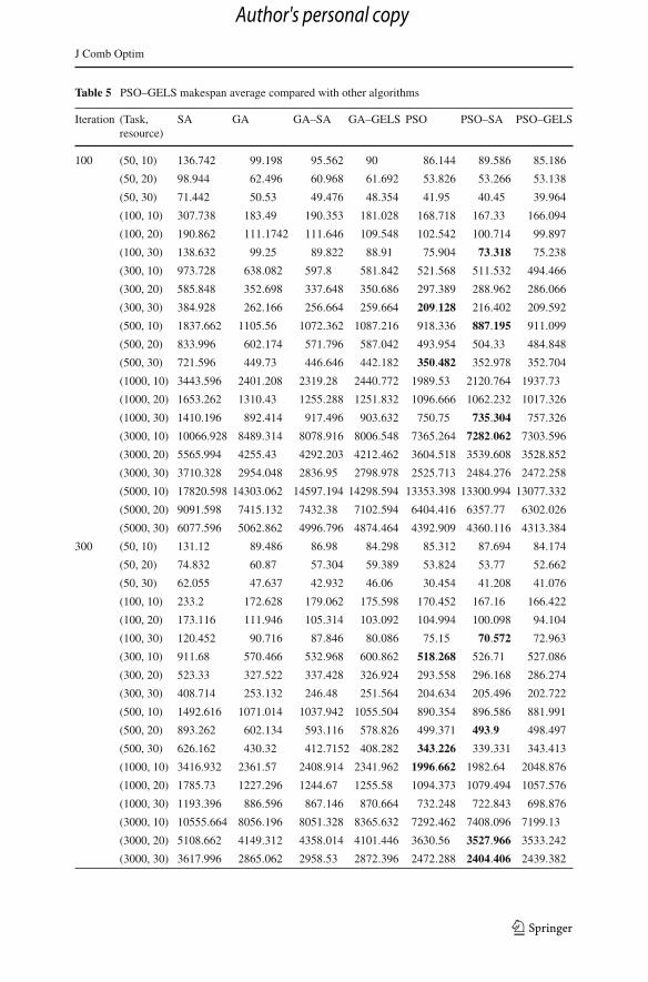
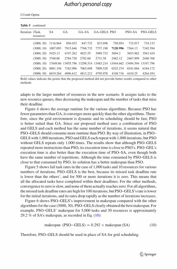
To show the significant performance of our PSO–GELS algorithm, we compared itwith the SA, GA–SA, GA–GELS, GA, PSO–SA, and PSO algorithms under variousconditions, including different numbers of tasks and resources with different numbersof iterations. The PSO–SA algorithm combines PSO and SA for solving the taskscheduling problem, GA–SA combines GA and SA, and GA–GELS combines GAand GELS. The algorithms were tested for various cases and the makespan, executiontime, and number of tasks that missed deadlines were calculated. Table 5 at the end ofthis article shows the makespan averages for the seven algorithms.

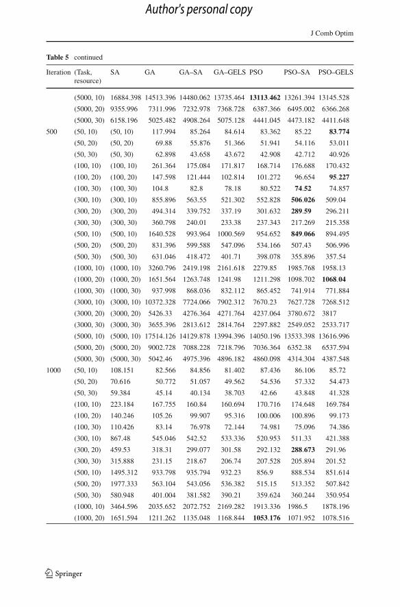
The results show that the makespan found by PSO–GELS is in most cases betterthan that found by the other algorithms. We expect a good scheduling algorithm toallocate resources to tasks with a minimal total runtime. Since PSO’s convergenceis faster than that of the GA, it is more suitable for grid scheduling. Moreover, PSOfound better solutions than the GA. Because PSO cannot search locally, we combinedit with the GELS method. The results show that PSO–GELS is better than PSO–SA;this is because GELS searches the problem space intelligently and does not work asthe SA method does—searching quickly to find solutions with better goal functionvalues—but does its job by examining present solutions; as a result, its algorithmicconvergence is faster and it is able to find adequate solutions.

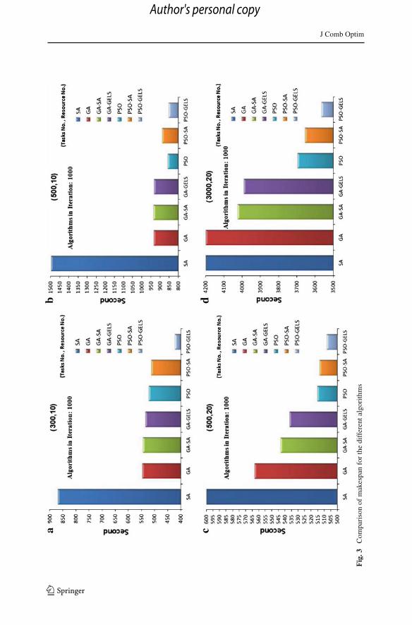
Figure 3a–d shows the makespan obtained by our proposed method compared withthe other algorithms for 1,000 iterations on 10 and 20, resources for various numbersof input tasks. As can be seen in the figure, as the number of input tasks increasesand the problem space grows, PSO–GELS performs better than the other algorithms.When the number of tasks increases to greater than 500, PSO–GELS produces asmaller makespan compared to the other algorithms. Additionally, when the numberof available resources in the system changes, increasing from 10 to 20, PSO–GELS

123


J Comb Optim

Table 5 PSO–GELS makespan average compared with other algorithms

Iteration (Task,resource)

SA GA GA–SA GA–GELS PSO PSO–SA PSO–GELS

100 (50, 10) 136.742 99.198 95.562 90 86.144 89.586 85.186

(50, 20) 98.944 62.496 60.968 61.692 53.826 53.266 53.138

(50, 30) 71.442 50.53 49.476 48.354 41.95 40.45 39.964

(100, 10) 307.738 183.49 190.353 181.028 168.718 167.33 166.094

(100, 20) 190.862 111.1742 111.646 109.548 102.542 100.714 99.897

(100, 30) 138.632 99.25 89.822 88.91 75.904 73.318 75.238

(300, 10) 973.728 638.082 597.8 581.842 521.568 511.532 494.466

(300, 20) 585.848 352.698 337.648 350.686 297.389 288.962 286.066

(300, 30) 384.928 262.166 256.664 259.664 209.128 216.402 209.592

(500, 10) 1837.662 1105.56 1072.362 1087.216 918.336 887.195 911.099

(500, 20) 833.996 602.174 571.796 587.042 493.954 504.33 484.848

(500, 30) 721.596 449.73 446.646 442.182 350.482 352.978 352.704

(1000, 10) 3443.596 2401.208 2319.28 2440.772 1989.53 2120.764 1937.73

(1000, 20) 1653.262 1310.43 1255.288 1251.832 1096.666 1062.232 1017.326

(1000, 30) 1410.196 892.414 917.496 903.632 750.75 735.304 757.326

(3000, 10) 10066.928 8489.314 8078.916 8006.548 7365.264 7282.062 7303.596

(3000, 20) 5565.994 4255.43 4292.203 4212.462 3604.518 3539.608 3528.852

(3000, 30) 3710.328 2954.048 2836.95 2798.978 2525.713 2484.276 2472.258

(5000, 10) 17820.598 14303.062 14597.194 14298.594 13353.398 13300.994 13077.332

(5000, 20) 9091.598 7415.132 7432.38 7102.594 6404.416 6357.77 6302.026

(5000, 30) 6077.596 5062.862 4996.796 4874.464 4392.909 4360.116 4313.384

300 (50, 10) 131.12 89.486 86.98 84.298 85.312 87.694 84.174

(50, 20) 74.832 60.87 57.304 59.389 53.824 53.77 52.662

(50, 30) 62.055 47.637 42.932 46.06 30.454 41.208 41.076

(100, 10) 233.2 172.628 179.062 175.598 170.452 167.16 166.422

(100, 20) 173.116 111.946 105.314 103.092 104.994 100.098 94.104

(100, 30) 120.452 90.716 87.846 80.086 75.15 70.572 72.963

(300, 10) 911.68 570.466 532.968 600.862 518.268 526.71 527.086

(300, 20) 523.33 327.522 337.428 326.924 293.558 296.168 286.274

(300, 30) 408.714 253.132 246.48 251.564 204.634 205.496 202.722

(500, 10) 1492.616 1071.014 1037.942 1055.504 890.354 896.586 881.991

(500, 20) 893.262 602.134 593.116 578.826 499.371 493.9 498.497

(500, 30) 626.162 430.32 412.7152 408.282 343.226 339.331 343.413

(1000, 10) 3416.932 2361.57 2408.914 2341.962 1996.662 1982.64 2048.876

(1000, 20) 1785.73 1227.296 1244.67 1255.58 1094.373 1079.494 1057.576

(1000, 30) 1193.396 886.596 867.146 870.664 732.248 722.843 698.876

(3000, 10) 10555.664 8056.196 8051.328 8365.632 7292.462 7408.096 7199.13

(3000, 20) 5108.662 4149.312 4358.014 4101.446 3630.56 3527.966 3533.242

(3000, 30) 3617.996 2865.062 2958.53 2872.396 2472.288 2404.406 2439.382

123


J Comb Optim

Table 5 continued



(5000, 10) 16884.398 14513.396 14480.062 13735.464 13113.462 13261.394 13145.528

(5000, 20) 9355.996 7311.996 7232.978 7368.728 6387.366 6495.002 6366.268

(5000, 30) 6158.196 5025.482 4908.264 5075.128 4441.045 4473.182 4411.648

500 (50, 10) (50, 10) 117.994 85.264 84.614 83.362 85.22 83.774

(50, 20) (50, 20) 69.88 55.876 51.366 51.941 54.116 53.011

(50, 30) (50, 30) 62.898 43.658 43.672 42.908 42.712 40.926

(100, 10) (100, 10) 261.364 175.084 171.817 168.714 176.688 170.432

(100, 20) (100, 20) 147.598 121.444 102.814 101.272 96.654 95.227

(100, 30) (100, 30) 104.8 82.8 78.18 80.522 74.52 74.857

(300, 10) (300, 10) 855.896 563.55 521.302 552.828 506.026 509.04

(300, 20) (300, 20) 494.314 339.752 337.19 301.632 289.59 296.211

(300, 30) (300, 30) 360.798 240.01 233.38 237.343 217.269 215.358

(500, 10) (500, 10) 1640.528 993.964 1000.569 954.652 849.066 894.495

(500, 20) (500, 20) 831.396 599.588 547.096 534.166 507.43 506.996

(500, 30) (500, 30) 631.046 418.472 401.71 398.078 355.896 357.54

(1000, 10) (1000, 10) 3260.796 2419.198 2161.618 2279.85 1985.768 1958.13

(1000, 20) (1000, 20) 1651.564 1263.748 1241.98 1211.298 1098.702 1068.04

(1000, 30) (1000, 30) 937.998 868.036 832.112 865.452 741.914 771.884

(3000, 10) (3000, 10) 10372.328 7724.066 7902.312 7670.23 7627.728 7268.512

(3000, 20) (3000, 20) 5426.33 4276.364 4271.764 4237.064 3780.672 3817

(3000, 30) (3000, 30) 3655.396 2813.612 2814.764 2297.882 2549.052 2533.717

(5000, 10) (5000, 10) 17514.126 14129.878 13994.396 14050.196 13533.398 13616.996

(5000, 20) (5000, 20) 9002.728 7088.228 7218.796 7036.364 6352.38 6537.594

(5000, 30) (5000, 30) 5042.46 4975.396 4896.182 4860.098 4314.304 4387.548

1000 (50, 10) 108.151 82.566 84.856 81.402 87.436 86.106 85.72

(50, 20) 70.616 50.772 51.057 49.562 54.536 57.332 54.473

(50, 30) 59.384 45.14 40.134 38.703 42.66 43.848 41.328

(100, 10) 223.184 167.755 160.84 160.694 170.716 174.648 169.784

(100, 20) 140.246 105.26 99.907 95.316 100.006 100.896 99.173

(100, 30) 110.426 83.14 76.978 72.144 74.981 75.096 74.386

(300, 10) 867.48 545.046 542.52 533.336 520.953 511.33 421.388

(300, 20) 459.53 318.31 299.077 301.58 292.132 288.673 291.96

(300, 30) 315.888 231.15 218.67 206.74 207.528 205.894 201.52

(500, 10) 1495.312 933.798 935.794 932.23 856.9 888.534 851.614

(500, 20) 1977.333 563.104 543.056 536.382 515.15 513.352 507.842

(500, 30) 580.948 401.004 381.582 390.21 359.624 360.244 350.954

(1000, 10) 3464.596 2035.652 2072.752 2169.282 1913.336 1986.5 1878.196

(1000, 20) 1651.594 1211.262 1135.048 1168.844 1053.176 1071.952 1078.516

123


J Comb Optim

Table 5 continued



(1000, 30) 1116.864 856.032 847.732 833.698 750.054 732.017 724.133

(3000, 10) 1007.093 7915.646 7768.732 7757.198 7120.996 7364.13 7345.594

(3000, 20) 5425.13 4197.262 4023.55 3989.732 3694.2 3653.962 3563.424

(3000, 30) 3760.06 2784.728 2782.68 2731.58 2482.12 2467.899 2448.768

(5000, 10) 17649.86 13955.796 13298.514 13483.214 13444.662 13494.594 13347.796

(5000, 20) 8881.194 7182.096 7065.698 7009.528 6525.274 6541.064 6344.172

(5000, 30) 6019.264 4896.612 4813.212 4795.078 4348.716 4410.25 4264.454

Bold values indicate the points that the proposed method did not provide better results compared to othermethods

adapts to the larger number of resources in the new scenario. It assigns tasks to thenew resource queues, thus decreasing the makespan and the number of tasks that misstheir deadline.

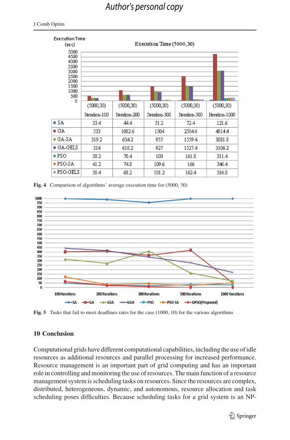
Figure 4 shows the average runtime for the various algorithms. Because PSO hasfewer parameters than GA, it converges more quickly than the other algorithms. There-fore, since the grid environment is dynamic and its scheduling should be fast, PSOis better suited than GA. Since our proposed method uses a combination of PSOand GELS and each method has the same number of iterations, it seems natural thatPSO–GELS should consume more runtime than PSO. By way of illustration, in PSO–GELS with 1,000 iterations, PSO and GELS each repeat with 1,000 iterations, but PSOwithout GELS repeats only 1,000 times. The results show that although PSO–GELSrepeated more instructions than PSO, its execution time is close to PSO’s. PSO–GEL’sexecution time is also better than the execution time of PSO–SA, even though bothhave the same number of repetitions. Although the time consumed by PSO–GELS isclose to that consumed by PSO, its solution has a better makespan than PSO.

Figure 5 shows fail task rates in the case of 1,000 tasks and 10 resources for variousnumbers of iterations. PSO–GELS is the best, because its missed task deadline rateis lower than the others’, and for 500 or more iterations it is zero. This means thatall the allocated tasks have completed within their deadlines. For the other methods,convergence to zero is slow, and none of them actually reaches zero. For all algorithms,the missed task deadline rates are high for 100 iterations, but PSO–GELS’s rate is lowerfor the initial iterations, and its rates drop rapidly as the number of iterations increases.

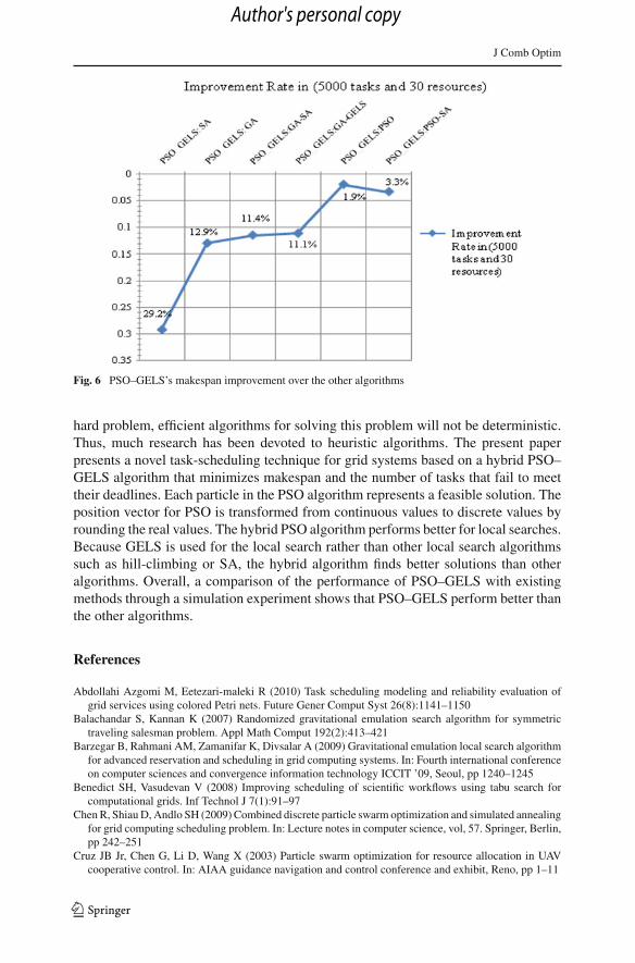
Figure 6 shows PSO–GELS’s improvement in makespan compared with the otheralgorithms for the case (5000, 30). PSO–GELS clearly obtained the best makespan. Forexample, PSO–GELS’ makespan for 5,000 tasks and 30 resources is approximately29.2 % of SA’s makespan, as recorded in Eq. (10):

makespan (PSO−GELS) = 0.292 × makespan (SA) (10)

Therefore, PSO–GELS should be used in place of SA for grid scheduling.

123


J Comb Optim

Fig

.3C

ompa

riso

nof

mak

espa

nfo

rth

edi

ffer

enta

lgor

ithm

s

123


J Comb Optim

Fig. 4 Comparison of algorithms’ average execution time for (5000, 30)

Fig. 5 Tasks that fail to meet deadlines rates for the case (1000, 10) for the various algorithms

10 Conclusion

Computational grids have different computational capabilities, including the use of idleresources as additional resources and parallel processing for increased performance.Resource management is an important part of grid computing and has an importantrole in controlling and monitoring the use of resources. The main function of a resourcemanagement system is scheduling tasks on resources. Since the resources are complex,distributed, heterogeneous, dynamic, and autonomous, resource allocation and taskscheduling poses difficulties. Because scheduling tasks for a grid system is an NP-

123


J Comb Optim

Fig. 6 PSO–GELS’s makespan improvement over the other algorithms

hard problem, efficient algorithms for solving this problem will not be deterministic.Thus, much research has been devoted to heuristic algorithms. The present paperpresents a novel task-scheduling technique for grid systems based on a hybrid PSO–GELS algorithm that minimizes makespan and the number of tasks that fail to meettheir deadlines. Each particle in the PSO algorithm represents a feasible solution. Theposition vector for PSO is transformed from continuous values to discrete values byrounding the real values. The hybrid PSO algorithm performs better for local searches.Because GELS is used for the local search rather than other local search algorithmssuch as hill-climbing or SA, the hybrid algorithm finds better solutions than otheralgorithms. Overall, a comparison of the performance of PSO–GELS with existingmethods through a simulation experiment shows that PSO–GELS perform better thanthe other algorithms.

References

Abdollahi Azgomi M, Eetezari-maleki R (2010) Task scheduling modeling and reliability evaluation ofgrid services using colored Petri nets. Future Gener Comput Syst 26(8):1141–1150

Balachandar S, Kannan K (2007) Randomized gravitational emulation search algorithm for symmetrictraveling salesman problem. Appl Math Comput 192(2):413–421

Barzegar B, Rahmani AM, Zamanifar K, Divsalar A (2009) Gravitational emulation local search algorithmfor advanced reservation and scheduling in grid computing systems. In: Fourth international conferenceon computer sciences and convergence information technology ICCIT ’09, Seoul, pp 1240–1245

Benedict SH, Vasudevan V (2008) Improving scheduling of scientific workflows using tabu search forcomputational grids. Inf Technol J 7(1):91–97

Chen R, Shiau D, Andlo SH (2009) Combined discrete particle swarm optimization and simulated annealingfor grid computing scheduling problem. In: Lecture notes in computer science, vol, 57. Springer, Berlin,pp 242–251

Cruz JB Jr, Chen G, Li D, Wang X (2003) Particle swarm optimization for resource allocation in UAVcooperative control. In: AIAA guidance navigation and control conference and exhibit, Reno, pp 1–11

123


J Comb Optim

Cruz-Chavez M, Rodríguez-Leon A, Avila-Melgar E, Juarez-Perez F, Cruz-Rosales M, Rivera-Lopez R(2010) Genetic-annealing algorithm in grid environment for scheduling problems. In: Security-enrichedurban computing and smart grid communications in computer and information science, vol 78. springer,New York, pp 1–9

Eberhat R, Kennedy J (1995) A new optimizer using particle swarm theory. In: Sixth international sympo-sium on micro machine and human science, Piscataway, pp 39–43

Foster I, Kesselman C, Nick J, Tuecke S (2002) The physiology of the grid: an open grid services architecturefor distributed systems integration. Computer 35(6):1–4

Gao Y, Rong HQ, Huang JZ (2005) Adaptive grid job scheduling with genetic algorithms. Future GenerComput Syst 21:151–161

Garg SK, Buyya R, Siegel HJ (2010) Time and cost trade-off management for scheduling parallel applica-tions on utility Grids. Future Gener Comput Syst 26:1344–1355

Izakian H, Tork Ladani B, Zamanifar K, Abraham A (2009) A novel particle swarm optimization approachfor grid job scheduling. Commun Comput Inf Sci 31:100–109

Joshua Samuel Raj R, Vasudevan V (2011) Beyond simulated annealing in grid scheduling. Int J ComputSci Eng 3(3):1312–1318

Liu H, Abraham A, Hassanien A (2010) Scheduling jobs on computational grids using a fuzzy particleswarm optimization algorithm. Future Gener Comput Syst 26:1336–1343

Maheswaran M (1999) Dynamic mapping of a class of independent tasks onto heterogeneous computingsystems. J Parallel Distributed Comput 59(2):107–131

Mathiyalagan P, Dhepthie UR, Sivanandam SN (2010) Grid scheduling using enhanced PSO algorithm. IntJ Comput Sci Eng 2(2):140–145

Orosz ZE, Jacobson SH (2002) Analysis of static simulated annealing algorithm. J Optim Theory Appl115:165–182

Padmavathi S, Mercy shalinie S (2010) Dag scheduling on cluster of workstations using hybrid particleswarm optimization. In: First international conference on emerging trends in engineering and technologyICETET ’08, vol 10, Mawson Lakes, no 6, pp 384–389

Pooranian Z, Harounabadi A, Shojafar M, Hedayat N (2011) New hybrid algorithm for task scheduling ingrid computing to decrease missed task. World Acad Sci Eng Technol 55:924–928

Pooranian Z, Shojafar M, Javadi B (2012) Independent task scheduling in grid computing based on queenbee algorithm. IAES Int J Artif Intell 1(4):171–181

Pooranian Z, Shojafar M, Abawajy JH, Singhal M (2013a) GLOA: a new job scheduling algorithm for gridcomputing. Int J Artif Intell Interact Multimed 2(1):59–64

Pooranian Z, Shojafar M, Tavoli R, Singhal M, Abraham A (2013b) A hybrid meta-heuristic algorithm forjob scheduling on computational grids. Inform J 37(2):157–164

Shiau Der-Fang (2011) A hybrid particle swarm optimization for a university course scheduling problemwith flexible preferences. Expert Syst Appl 38:235–248

Shiau D, Huang Y (2012) A hybrid two-phase encoding particle swarm optimization for total weightedcompletion time minimization in proportionate flexible flow shop scheduling. Int J Adv Manuf Technol58(1):339–357

Shi Y, Eberhat R (1998) Parameter selection in particle swarm optimization. In: Proceedings of the 7thannuals conference on evolutionary programming. Springer, Berlin, pp 591–600

Shi Y, Eberhat R (1999) Empirical study of particle swarm optimization. In: Proceedings of the IEEEcongress on evolutionary computation, vol 3. IEEE Press, Los Alamitos, pp 1945–1950

Shojafar M, Barzegar S, Meybodi MR (2010) A new method on resource scheduling in grid systems basedon hierarchical stochastic Petri net. In: Proceedings of third international conference on computer andelectrical engineering (ICCEE 2010), Chengdu, pp 175–180

Shojafar M, Pooranian Z, Abawajy JH, Meybodi MR (2013) An efficient scheduling method for grid systemsbased on a hierarchical stochastic Petri net. J Comput Sci Eng 7(1):44–52

Sivanandam SN, Visalakshi P (2007) Multiprocessor scheduling using hybrid particle swarm optimizationwith dynamically varying inertia. Int J Comput Sci Appl 4(3):95–106

Sullivan WT, Werthimer D, Bowyer S, Cobb J, Gedye D, Anderson D (1997) A new major SETI projectbased on Project Serendip data and 100000 personal computers. In: Proceedings of the fifth internationalconference on bioastronomy, Bologna, no 61, p 729

Tao Q, Chang H, Yi Y, Gu CH, Li W (2011) A rotary chaotic PSO algorithm for trustworthy scheduling ofa grid workflow. Comput Oper Res 38:824–836

Voudouris CH, Tsang E (1995) Guided local search. Eur J Oper Res 16(3):46–50

123


J Comb Optim

Webster B (2004) Solving combinatorial optimization problems using a new algorithm based on gravitationalattraction. PhD thesis, Florida Institute of Technology, Melbourne

Weijun X, Zhiming W, Wei ZH, Genke Y (2004) A new hybrid optimization algorithm for the job-shopscheduling problem. In: Proceeding of the 2004 American control conference, vol 6, Boston, pp 5552–5557

Xhafa F, Gonzalez J, Dahal K, Abraham A (2009) A GA(TS) hybrid algorithm for scheduling in compu-tational grids. In: Hybrid artificial intelligence systems. Lecture notes in computer science, vol 5572.Springer, Berlin, pp 285–292

Yan-ping B, Wei ZH, Jin-shou Y (2008) An improved PSO algorithm and its application to grid schedulingproblem. International symposium on computer science and computational technology ISCSCT ’08,Shanghai, pp 352–355

Yusof M, Badak K, Stapa M (2010) Achieving of tabu search algorithm for scheduling technique in gridcomputing using GridSim simulation tool: multiple jobs on limited resource. Int J Grid DistributedComput 3(4):19–32

Zhang L, Chen Y, Sun R, Jing SH, Yang B (2008) A task scheduling algorithm based on PSO for gridcomputing. Int J Comput Intell Res 4(1):37–43

123


Documents

An efficient meta-heuristic algorithm for grid computing