Embed Size (px)
Citation preview

An Efficient Precoder Design for Multiuser MIMO Cognitive RadioNetworks with Interference Constraints
Nguyen, V-D., Duong, T. Q., Tran, L-N., Shin, O-S., & Farrell, R. (2016). An Efficient Precoder Design forMultiuser MIMO Cognitive Radio Networks with Interference Constraints. IEEE Transactions on VehicularTechnology. https://doi.org/10.1109/TVT.2016.2602844
Published in:IEEE Transactions on Vehicular Technology
Document Version:Peer reviewed version
Queen's University Belfast - Research Portal:Link to publication record in Queen's University Belfast Research Portal
Publisher rightsCopyright 2016 IEEE. Personal use of this material is permitted. Permission from IEEE must be obtained for all other users, includingreprinting/ republishing this material for advertising or promotional purposes, creating new collective works for resale or redistribution toservers or lists, or reuse of any copyrighted components of this work in other works.
General rightsCopyright for the publications made accessible via the Queen's University Belfast Research Portal is retained by the author(s) and / or othercopyright owners and it is a condition of accessing these publications that users recognise and abide by the legal requirements associatedwith these rights.
Take down policyThe Research Portal is Queen's institutional repository that provides access to Queen's research output. Every effort has been made toensure that content in the Research Portal does not infringe any person's rights, or applicable UK laws. If you discover content in theResearch Portal that you believe breaches copyright or violates any law, please contact [email protected].
Download date:14. Mar. 2022

1
An Efficient Precoder Design for Multiuser MIMOCognitive Radio Networks with Interference
ConstraintsVan-Dinh Nguyen, Le-Nam Tran, Member, IEEE, Trung Q. Duong, Senior Member, IEEE,
Oh-Soon Shin, Member, IEEE, and Ronan Farrell, Member, IEEE
Abstract—We consider a linear precoder design for an un-derlay cognitive radio multiple-input multiple-output broadcastchannel, where the secondary system consisting of a secondarybase-station (BS) and a group of secondary users (SUs) is allowedto share the same spectrum with the primary system. All thetransceivers are equipped with multiple antennas, each of whichhas its own maximum power constraint. Assuming zero-forcingmethod to eliminate the multiuser interference, we study the sumrate maximization problem for the secondary system subject toboth per-antenna power constraints at the secondary BS and theinterference power constraints at the primary users. The problemof interest differs from the ones studied previously that oftenassumed a sum power constraint and/or single antenna employedat either both the primary and secondary receivers or theprimary receivers. To develop an efficient numerical algorithm,we first invoke the rank relaxation method to transform theconsidered problem into a convex-concave problem based on adownlink-uplink result. We then propose a barrier interior-pointmethod to solve the resulting saddle point problem. In particular,in each iteration of the proposed method we find the Newtonstep by solving a system of discrete-time Sylvester equations,which help reduce the complexity significantly, compared tothe conventional method. Simulation results are provided todemonstrate fast convergence and effectiveness of the proposedalgorithm.
Index Terms—MIMO, broadcast channel, beamforming, cog-nitive radio, zero-forcing, sum rate maximization.
I. INTRODUCTION
Radio frequency spectrum has recently become a scarce andexpensive wireless resource due to the ever increasing demandof multimedia services. Nevertheless, it has been reported in[1] that the majority of licensed users are idle at any given timeand location. To significantly improve spectrum utilization,cognitive radio (CR) is widely considered as a promisingapproach. There are two famous CR models, namely oppor-tunistic spectrum access model and spectrum sharing model.
V.-D. Nguyen and O.-S. Shin are with the School of Electronic Engi-neering, Soongsil University, Seoul 06978, Korea (e-mail: nguyenvandinh,[email protected]).
T. Q. Duong is with the School of Electronics, Electrical Engineering andComputer Science, Queen’s University Belfast, Belfast BT7 1NN, UnitedKingdom (e-mail: [email protected]).
L.-N. Tran and R. Farrell are with the Department of Electronic En-gineering, Maynooth University, Co. Kildare, Ireland (e-mail: ltran, [email protected]).
This work was supported in part by Basic Research Laboratories (BRL)through NRF grant funded by the MSIP (No. 2015056354). The work ofT. Q. Duong was supported in part by the U.K. Royal Academy of EngineeringFellowship under Grant RF1415\14\22 and by the Newton Institutional Linkunder Grant ID 172719890.
In the former, the secondary users (SUs, unlicensed users)are allowed to use the frequency bands of the primary users(PUs, licensed users) only when these bands are not occupied[2]–[6]. In the latter, the PUs have prioritized access to theavailable radio spectrum, while the SUs have restricted accessand need to avoid causing detrimental interference to theprimary receivers [7]–[9]. Towards this end, several powerfultechniques such as spectrum sensing and beamforming design,have been used to protect the PUs from the interference fromthe SUs and to meet quality-of-service (QoS) requirements[10]–[13].
It is well-known that transmit beamforming has enormouspotential to improve the capacity of wireless communicationsystems without requiring extra bandwidth or transmit power.In fact, a popular method to control the interference that hasbeen widely used in the literature is based on zero-forcing(ZF) technique, which places null spaces at the beamformingvector of each co-channel receiver. Specifically, successivezero-forcing dirty paper coding (SZF-DPC) was introducedin [14] for single-antenna receivers and was extended tomultiple-antenna receivers in [15]. Inspired by these twoworks, the authors in [16], [17] proposed efficient numericalmethods based on a barrier method to solve the throughputmaximization problem. These approaches were shown to havea superior convergence behavior compared to a two-stageiterative method based on the dual subgradient method [18].
The throughput maximization of a CR network was opti-mally solved in [11], which considered a single secondarymultiple-input multiple-output (MIMO)/multiple-input single-output (MISO) link under the constraint of opportunisticspectrum sharing. Multiple antennas are exploited at the sec-ondary transmitter to optimally trade off between attaining themaximal throughput and meeting the interference thresholdat the primary receivers. The throughput of the SU linkwas studied with instantaneous or average interference-powerconstraint at a single PU in [19]. When multiple SUs accessa single-frequency which is licensed to one PU, a QoSconstraint for each secondary link is solved efficiently using ageometric programming method under the interference-powerconstraint at some measured point [20], [21]. The authorsin [22] considered maximizing the smallest weighted rateand proposed distributed algorithms for optimal beamformingand rate allocation. The channel capacity of CR networkswith two users was presented in [23], where the cognitiveuser is assumed to know the message of the primary user

2
non-causally prior to transmissions. The impact of averageinterference power and peak interference power constraints onthe ergodic capacity of CR networks was compared in [24]. In[25], an enhanced spectrum sensing scheme was proposed toimprove the optimal power allocation strategy in CR networks.In parallel lines, beamforming design technique was appliedto control the total amount of interference caused by thesecondary transmitter, thereby enhancing the channel capacityof CR MIMO networks [26], [27].
The sum rate (SR) maximization problem of CR has beena classical one in wireless system design [28]–[31]. In par-ticular, the authors in [28] considered the weighted sum rate(WSR) maximization problem for CR multiple-SUs MIMObroadcast channel (BC) under the sum power constraint andthe interference power constraints. The problem is shownto be a nonconvex problem but can be transformed into anequivalent convex CR MIMO multiple access channel (MAC)problem via the general BC-MAC duality result. The problemof WSR maximization for multiple MISO SUs in the presenceof multiple primary receivers was addressed in [29], where aniterative algorithm based on the subgradient method was pro-posed to determine the beamforming vectors. For the MIMOad hoc CR network considered in [30], a semidistributedalgorithm and a centralized algorithm based on geometricprogramming and network duality were introduced under theinterference constraint at the primary receivers in order toobtain a locally optimal linear precoder for the non-convexWSR maximization problem. In [31], the authors investigateda CR multiple-antenna two-way relay network, where optimalrelay beamforming and suboptimal beamforming vectors wereobtained based on the subspace projection and power controlalgorithms that are proposed to satisfy the power budget aswell as the interference power constraints. However, all ofthese algorithms generally have high computational complex-ity and slow convergence.
Very recently, the SR maximization for CR MISO-BC witha very large number of antennas at the secondary transmitterwas studied in [32]. For the general case, a low-complexitysuboptimal beamforming scheme based on partially-projectedregularized ZF beamforming was applied to obtain a closed-form beamformer, and then deterministic approximations forlarge system analysis were also derived. The authors in [33],[34] studied a WSR maximization problem with a collection ofmultiple PUs and SUs sharing a common frequency-flat fadingchannel. Under the interference power and transmit powerconstraint, a reformulation-relaxation technique was proposedto solve a convex optimization problem over a closed boundedconvex set in the rate domain to bound the optimal value,and a branch-and-bound algorithm is used to find a globallyoptimal solution to the WSR maximization problem. Mostof prior research on beamforming design for CR networksassumed that single antenna is employed at either both theprimary and secondary receivers or the primary receiver. To thebest of our knowledge, the SR maximization problem in moregeneral cases for CR MIMO-BC networks in the presence ofmultiple SUs and PUs is still an open research and has notbeen investigated previously.
In this paper we consider a CR network where the secondary
system consisting of a multiantenna BS sends data to multipleusers on its downlink channel while satisfying the interferencelimit that it may cause to the legitimate users of the primarysystem. We note that the capacity of the downlink transmissionof the secondary system can be achieved through DPC [35].However, DPC is difficult to implement in practice since itis a nonlinear precoding technique with high implementationcomplexity. In this paper we adopt ZF precoding which hasbeen widely used in the literature thanks to its simplicity andeffectiveness at the secondary base station (BS), and considerthe SR maximization problem subject to per-antenna powerconstraints (PAPC) at secondary BS and the interference powerconstraint at PUs. By a standard rank relaxation method, theprecoder design problem can be cast as a semidefinite programwhich can be solved by generic conic solvers such as SeDuMi[36] or SDPT3 [37]. However, we do not follow such approachfor the following two reasons. First, it provides little usefulinsights into the structure of the optimal precoder. Second,its computational complexity is generally very high sincespecifications of the considered problem are not exploited. Inthis paper, our contributions include the followings
• We reformulate the SR maximization problem for theconsidered CR MIMO system subject to PAPCs and in-terference constraints into a concave-convex (also knownas minimax) program by extending a BC-MAC dualityresult. To do this we first apply a standard rank relaxationmethod and then prove that the relaxation is tight. Inparticular, we show that the PAPCs and interferenceconstraints will become equality constraints in the derivedconvex-concave program.
• We customize the barrier method to find a saddle point(i.e., an optimal solution) of the convex-concave program.The proposed algorithm is basically an iterative Newton-type method which is customized to exploit the specialfeatures of the design problem. Explicitly, in each it-eration to find the Newton step, we arrive at a systemof Sylvester equations which is less complex to solve,compared to a generic method based on solving a systemof linear equations.
• We provide extensive numerical results to justify thenovelty of the algorithm and compare its performancewith suboptimal solutions. In particular, the numericalresults demonstrate a superlinear convergence rate ofthe proposed algorithm and superior performance onachievable sum rate over the suboptimal solutions.
The rest of the paper is organized as follows. System modeland the formulation of the SR maximization problem aredescribed in Section II. In Section III, we present the proposedalgorithm to solve the considered problem. Numerical resultsare provided in Section IV, and Section V concludes the paper.
Notations: Bold lower and upper case letters representvectors and matrices, respectively; HH and HT are Hermitianand normal transpose of H, respectively; tr(H) and |H| arethe trace and the determinant of H, respectively; IN representsan N × N identity matrix. [x]i is the ith entry of vector x.[H]i,j is the entry at the ith row and jth column of H. en is thenth unit vector (all entries are zero except for the nth element

3
BS(SU)
N
SUK
nK
n1
SU1
n1 nM
PU1 PUM
HK
H1
G1 GM
Data link Interference link
Figure 1: A cognitive network model with multiple SUs andPUs.
which is 1). diag(x), where x is a vector, denotes a diagonalmatrix with diagonal elements of x. The notation X 0represents that X is a positive semidefinite matrix. N (H)denotes the null space of H and λmax(X) is the maximumeigenvalue of X.
II. SYSTEM MODEL AND PROBLEM FORMULATION
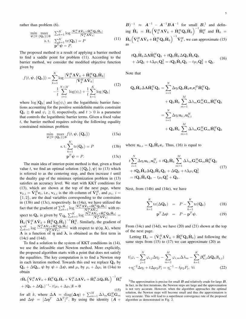
We consider a cognitive transmission scenario where an N -antenna secondary BS sends data to K SUs in the presence ofM PUs as shown in Fig. 1. The secondary system is allowedto share the same spectrum band licensed to the primarysystem. In an underlay cognitive network, the secondaryBS must adapt its transmit power to satisfy an interferencepower constraint at the mth PU which is denoted by Im,for m = 1, 2, · · · ,M . The numbers of receive antennas atthe kth SU and the mth PU are denoted by nk and nm,respectively, and their channel matrices (to the secondaryBS) are represented by Hk ∈ Cnk×N , for k = 1, · · · ,K,and Gm ∈ Cnm×N , for m = 1, · · · ,M , respectively. Weassume that Hk, ∀k and Gm, ∀m remains constant during atransmission block and change independently from one blockto another. We further assume that the channel matrices canbe perfectly known at the secondary BS, using a genie addedfeedback. Though this assumption is quite ideal, it has beenconsidered in [28], [29], [32] to study their problems of interestin the context of CR networks. In reality, perfect channelestimation is hardly achieved and thus the results obtained inthis paper may act as an upper bound on the SR performancefor the secondary transmission in an underlay CR network.
In the considered system, linear precoding is employed atthe secondary BS to transmit data to the SUs. Specifically, thevector of transmitted symbols of the kth SU, denoted by xk, ismultiplied by the precoder Tk ∈ CN×Lk , Lk ≤ min(N,nk),before being transmitted. We assume that E[xkx
Hk ] = I.
In this way, the complex baseband transmitted signal at the
secondary BS can be expressed as
x =
K∑
k=1
Tkxk (1)
and the received signal at the kth SU is given by
yk = HkTkxk +∑
j 6=k
HkTjxj + zk (2)
where zk ∈ Cnk×1 is the background noise with distributionCN (0, Ink
). According to ZF precoding, we need to designTj such that HkTj = 0 for all j 6= k. Consequently, theproblem of SR maximization for cognitive transmission ismathematically formulated as
maxTk
K∑
k=1
log |I + HkTkTHk HH
k | (3a)
s. t. HkTj = 0, ∀j 6= k (3b)K∑
k=1
[TkTHk ]n,n ≤ Pn, ∀n ∈ N (3c)
K∑
k=1
tr(GmTkTHk GH
m) ≤ Im, ∀m ∈M (3d)
whereN , 1, 2, · · · , N andM , 1, 2, · · · ,M. Here, theconstraint in (3c) is the power constraints for the nth antennaat the secondary BS. We remark that an antenna is oftenequipped with its own power amplifier (PA). Thus, we mayneed to limit the maximum transmit power on each antenna forit to operate within the linear region of the PA, which is morepower efficient [39], [40]. The per-antenna power constraints(PAPCs) in (3c) different from those considered in [28], [32],but we note that the proposed solution introduced in this paperalso applies to the sum power constraint (SPC) after slightmodifications. This will be elaborated in the Appendix. Infact the interference from the secondary BS to a particularPU is a matrix, which is non-degrading. This is different fromthe case of PUs with single antenna in which the interferenceis a scalar, referred to as interference temperature [28]. Theconstraints in (3d) indicate that the sum of all eigenvaluesof the resulting interference matrix should be less than apredetermined interference threshold Im at the mth PU. Wecan rewrite (3d) as
∑nm
i=1
∑Kk=1 gm,iTkT
Hk g
Hm,i ≤ Im, where
gm,i ∈ C1×N denotes the channel from the secondary BSto the ith receive antenna of the mth PU. We note thatthe term
∑Kk=1 gm,iTkT
Hk g
Hm,i represents the interference
temperature at the ith antenna of the mth PU. In this way,(3d) implies that the sum of the interference temperatures ofall antennas at the mth PU should be smaller than or equalto a predetermined threshold. There are possibly other waysto control the interference generated by the secondary system.For example, we may force the maximum eigenvalue or thedeterminant (equivalent to the product of eigenvalues) of theinterference matrix to be smaller than a threshold. We remarkthat all these ways of controlling the interference term are thesame for single-antenna PUs.
To further simplify (3), let Hk =[HT
1 · · ·HTk−1 HT
k+1 · · ·HTK ]T ∈ C(nR−nk)×N , where

4
nR =∑Kk=1 nk is the total number of receive antennas.
The condition for (3b) to be feasible is that N (Hk) has adimension larger than zero, i.e., nR−nk > 0, for all k. In thispaper, we assume that the problem design in (3) is feasible,which can be met when N −∑i6=k ni ≥ nk and the channelmatrices of the SUs and PUs have sufficiently low correlationdegree. Let Vk be the null space of Hk, then Vk ∈ CN×nk
is a basis of N (Hk), where nk = N −∑i 6=k ni. Then wecan write Tk = VkTk, where Tk are the solutions to thefollowing problem
maxTk
K∑
k=1
log |I + HkVkTkTHk VH
k HHk | (4a)
s. t.
K∑
k=1
[VkTkTHk VH
k ]n,n ≤ Pn, ∀n ∈ N (4b)
K∑
k=1
tr(GmkTkTHk GH
mk) ≤ Im,∀m ∈M (4c)
where Gmk , GmVk ∈ Cnm×nk . Note that the problem(4) is not a convex program and indeed different from [16],where only conventional MISO systems were considered, i.e.,without interference constraints. Moreover, we will solve (5)through a BC-MAC duality, in contrast to dealing with theprimal domain as done in [17]. Towards this end we considerthe following problem.
maxSk0
K∑
k=1
log |I + HkSkHHk | (5a)
s. t.
K∑
k=1
[VkSkVHk ]n,n ≤ Pn, ∀n ∈ N (5b)
K∑
k=1
tr(GmkSkGHmk) ≤ Im,∀m ∈M (5c)
rank(Sk) ≤ nk, ∀k (5d)
where Hk = HkVk ∈ Cnk×nk and Sk = TkTHk . Though (5)
is a nonconvex program, it can be solved to global optimalityby dropping the rank constraints in (5d) and then consideringthe so-called rank relaxed problem. We will prove shortly thatthe optimal solutions of the relaxed problem must satisfy therank constraints in (5d), meaning that the rank relaxation istight. Thus, from now onwards, we will consider the relaxedproblem of (5) in the sequel of the paper, instead of (5) in theoriginal form.
To solve the relaxed problem of (5), we can modify themethod presented in [18] which is based on the subgradientmethod. However, subgradient methods generally convergevery slow in practice. Herein we propose an efficient methodto solve it using a barrier method which is known to havesuperlinear convergence property.
III. PROPOSED ALGORITHM
In this section, we first transform the problem (5) intoan equivalent convex-concave problem [41, Section 10.3.4],thereby showing the structure of the optimal precoder Sk.
We then propose a numerical algorithm to solve the convex-concave problem by customizing interior-point methods to finda saddle point (i.e., an optimal solution). The development ofthe proposed algorithm is particularly based on the followingtheorem.
Theorem 1. Consider the following convex-concave problem.
minψ≥0
maxQk0
∑Kk=1 log
|VHk ΛVk+HH
k QkHk||VH
k ΛVk|
s. t.∑Kk=1 tr(Qk) ≤ P
pTψ ≤ P.(6)
where Λ = diag(η) +∑Mm=1 λmGH
mGm, ψ = [ηT λT ]T ,and p = [pT I
T]T . We note that the objective function in
(6) is convex in ψ for fixed Qk, and concave in Qk forfixed ψ, hence the name convex-concave. Let Ωk = VH
k ΛVk,and UkDkV
Hk be a singular value decomposition (SVD) of
HkΩ−1/2k where Dk is square and diagonal. Then, the optimal
solution Sk of (5) can be obtained from that of (6) as
Sk = Ω−1/2k VkU
Hk QkUkV
Hk Ω
−1/2k . (7)
Proof: Please refer to the Appendix.Remark 1. Theorem 1 is different but similar in many waysto Theorem 2 in [16] which is only dedicated to PAPCsand MISO cases. Our duality result in Theorem 1 can beviewed as an extension of the duality results in [16] to thecase of multiple linear constraints and MIMO cases. Sincerank(Qk) ≤ nk, it follows that rank(Sk) ≤ nk, which meansthe relaxed problem of (5) is equivalent to (4).Remark 2. Before proceeding further we provide someinsights into the convex-concave program in (6). Letf(ψ, Qk) ,
∑Kk=1 log
|VHk ΛVk+HH
k QkHk||VH
k ΛVk|, i.e., the objec-
tive of (6). Then a problem closely related to (6) is given by
maxQk0
minψ≥0
f(ψ, Qk)
s. t.∑Kk=1 tr(Qk) ≤ P
pTψ ≤ P.(8)
We can say that (ψ∗, Q∗k) is a solution to the convex-concave program or a saddle-point for the problem, if for allψ and Qk
f(ψ∗, Qk) ≤ f(ψ∗, Q∗k) ≤ f(ψ, Q∗k). (9)
Since f(ψ, Qk) is differentiable, the above inequality im-plies that the strong max-min property holds, i.e.,
maxQk
minψ
f(ψ, Qk) = minψ
maxQk
f(ψ, Qk). (10)
It is clear from the above discussions that solving (6)boils down to finding a saddle point for the convex-concaveproblem for which we will propose a computationally efficientalgorithm. First, as intermediate results when proving Theorem1 (see the steps from (42) to (48) in the Appendix), wecan set the inequality constraints to be equality ones withoutaffecting the optimality. Based on this observation, it is morecomputationally efficient1 to consider the following problem
1The equality constraints are generally easier to handle when using a barriermethod to solve an optimization problem. The reason is that we need tointroduce a barrier function (i.e. the log function in our case) to deal withinequality constrains, while we do not need to do so for equality constraints.
5
rather than problem (6).
minψ≥0
maxQk0
∑Kk=1 log
|VHk ΛVk+HH
k QkHk||VH
k ΛVk|
s. t.∑Kk=1 tr(Qk) = P
pTψ = P.
(11)
The proposed method is a result of applying a barrier methodto find a saddle point for problem (11). According to thebarrier method, we consider the modified objective functiongiven by
f(t,ψ, Qk) =
K∑
k=1
log|VH
k ΛVk + HHk QkHk|
|VHk ΛVk|
−1
t
N+M∑
i=1
log(ψi) +1
t
K∑
k=1
log |Qk|(12)
where log |Qk| and log(ψi) are the logarithmic barrier func-tions accounting for the positive semidefinite matrix constraintQk 0 and ψi ≥ 0, respectively, and t > 0 is a parameterthat controls the logarithmic barrier terms. Given a fixed valuet, the barrier method requires solving the following equalityconstrained minimax problem
minψ≥0
maxQk0
f(t,ψ, Qk) (13a)
s. t.
K∑
k=1
tr(Qk) = P (13b)
pTψ = P. (13c)
The main idea of interior-point method is that, given a fixedvalue t, we find an optimal solution (Qk,ψ) to (13) whichis referred to as the centering step, and then increase t untilthe duality gap of the minimax optimization problem in (13)satisfies an accuracy level. We start with KKT conditions for(13), which are shown at the top of the next page, wherevk,i = VH
k ei, i.e., vk,i is the ith column of VHk , and µi, i =
1, 2, are the dual variables corresponding to the constraintsin (13b) and (13c), respectively. In (14a), we have utilized thefact that the gradient of
∑Kk=1 log
|VHk ΛVk+HH
k QkHk||VH
k ΛVk|with re-
spect to Qk is given by ∇Qk
∑Kk=1 log
|VHk ΛVk+HH
k QkHk||VH
k ΛVk|=
Hk
(VHk ΛVk + HH
k QkHk
)−1HHk . Similarly, the gradient of∑K
k=1 log|VH
k ΛVk+HHk QkHk|
|VHk ΛVk|
with respect to ψ(η,λ), whereΛ is a function of η and λ, is obtained as the first term in(14c) and (14d).
To find a solution to the system of KKT conditions in (14),we use the infeasible start Newton method. More explicitly,the proposed algorithm starts with a point that does not satisfythe equalities. The key computation is to find a Newton stepin each iteration method. Towards this end we replace Qk byQk + ∆Qk, ψ by ψ + ∆ψ, and µi by µi + ∆µi in (14a) toobtain
tHk
(VHk ΛVk + HH
k QkHk + VHk ∆ΛVk + HH
k ∆QkHk
)−1
HHk
+ (Qk + ∆Qk)−1− t(µ1 + ∆µ1)I = 0(15)
for all k, where ∆Λ = diag(∆η) +∑Mm=1 ∆λmGH
mGm
and ∆ψ = [∆ηT ∆λT ]T . By using the identity (A +
B)−1 ≈ A−1 − A−1BA−1 for small B,2 and defin-
ing Hk = Hk
(VHk ΛVk + HH
k QkHk
)−1
HHk and Hk =
Hk
(VHk ΛVk+HH
k QkHk
)−1
VHk , we can approximate (15)
as
tQkHk∆ΛHHk Qk + tQkHk∆QkHkQk
+ ∆Qk + t∆µ1Q2k = tQkHkQk − tµ1Q
2k + Qk.
(16)
Note that
QkHk∆ΛHHk Qk =
N∑
i=1
∆ηiQkHkeieHi HH
k Qk
+ QkHk
M∑
m=1
∆λmGHmGmHH
k Qk
=N∑
i=1
∆ηiuk,iuHk,i
+ QkHk
M∑
m=1
∆λmGHmGmHH
k Qk
where uk,i = QkHkei. Thus, (16) is equal to
t
N∑
i=1
∆ηiuk,iuHk,i + tQkHk
M∑
m=1
∆λmGHmGmHH
k Qk
+ tQkHk∆QkHkQk + ∆Qk + t∆µ1Q2k
= tQkHkQk − tµ1Q2k + Qk.
(17)
Next, from (14b) and (14e), we have
K∑
k=1
tr(∆Qk) = P −K∑
k=1
tr(Qk) (18)
pT∆ψ = P − pTψ. (19)
From (14c) and (14d), we have (20) and (21) shown at the topof the next page.
Letting Πk =(VHk ΛVk + HH
k QkHk
)and following the
same steps from (15) to (17) we can approximate (20) as
t(ϕi −N∑
j=1
ϕi,j∆ηj −M∑
m=1
ϕi,m∆λm −K∑
k=1
βHk,i∆Qkβk,i)
+η−2i ∆ηi + t∆µ2Pi = η−1
i − tµ2Pi, ∀i (22)
2The approximation is precise for small B and relatively crude for large B.In fact, in the first iterations, the Newton steps are large and the approximationis not very accurate. However, when the algorithm approaches the optimalsolution, the Newton steps will become small and thus the approximation isvery accurate. This will lead to a superlinear convergence rate of the proposedalgorithm as demonstrated in Fig. 2.
6
Hk
(VHk ΛVk + HH
k QkHk
)−1HHk +
1
tQ−1k − µ1I = 0,∀k (14a)
K∑
k=1
tr(Qk) = P (14b)
K∑
k=1
vHk,i
[(VH
k ΛVk + HHk QkHk)−1 − (VH
k ΛVk)−1]vk,i −
1
tη−1i + µ2Pi = 0,∀i (14c)
K∑
k=1
tr(Gmk
[(VH
k ΛVk + HHk QkHk)−1 − (VH
k ΛVk)−1]GHmk
)− λ−1
m
t+ µ2Im = 0,∀m (14d)
pTψ = P. (14e)
t
K∑
k=1
vHk,i
[(VH
k ΛVk + HHk QkHk + VH
k ∆ΛVk + HHk ∆QkHk)−1 (20)
−(VHk ΛVk + VH
k ∆ΛVk)−1]vk,i − (ηi + ∆ηi)
−1 + t(µ2 + ∆µ2)Pi = 0, ∀i.
t
K∑
k=1
tr(Gmk
[(VH
k ΛVk + HHk QkHk + VH
k ∆ΛVk + HHk ∆QkHk)−1 (21)
−(VHk ΛVk + VH
k ∆ΛVk)−1]GHmk
)− (λm + ∆λm)−1 + t(µ2 + ∆µ2)Im = 0, ∀m.
where ϕi, ϕi,j , ϕi,m, and βk,i are, respectively, given by
ϕi =
K∑
k=1
vHk,i[Π−1k −
(VHk ΛVk
)−1]vk,i
ϕi,j =
K∑
k=1
|vHk,iΠ−1k VH
k ej |2 − |vHk,i(VHk ΛVk
)−1VHk ej |2
ϕi,m =
K∑
k=1
‖vHk,iΠ−1k GH
mk‖2 − ‖vHk,i(VHk ΛVk
)−1GHmk‖2
βk,i = HkΠ−1k vk,i.
(23)In the same way, (21) is approximated as
t(φm −
N∑
j=1
φm,j∆ηj −M∑
s=1
φm,s∆λs −K∑
k=1
tr(ΞHm,k∆QkΞm,k
))
+ λ−2m ∆λm + t∆µ2Im = λ−1
m − tµ2Im, ∀m(24)
where φm, φm,j , φm,s, and Ξm,k are, respectively, defined as
φm =
K∑
k=1
tr(Gmk
[Π−1k −
(VHk ΛVk
)−1]GHmk
)
φm,j =
K∑
k=1
tr(Gmk
[Π−1k VH
k ejeHj VkΠ
−1k
−(VHk ΛVk
)−1VHk eje
Hj Vk
(VHk ΛVk
)−1]GHmk
)
φm,s =
K∑
k=1
tr(Gmk
[Π−1k GH
skGskΠ−1k
−(VHk ΛVk
)−1GHskGsk
(VHk ΛVk
)−1]GHmk
)
Ξm,k = HkΠ−1k GH
mk.(25)
We can find the Newton steps for the optimization variablesby staking (17), (18), (19), (22), and (24) into a system oflinear equations. However such a conventional method requirescomplexity of O
(K3N6
)3 which is relatively high. In this
paper we instead follow a block elimination method [17], [41]which results in much lower complexity.
∆Qk = Σ(0)k +
N+M∑
i=1
∆ψiΣ(i)k + ∆µ1Σ
(N+M+1)k . (26)
For notational simplicity, in (27), (28), and (30), we ex-plicitly write (26) as ∆Qk = Σ
(0)k +
∑Ni=1 ∆ηiΣ
(i)k +∑M
m=1 ∆λmΣ(m)k + ∆µ1Σ
(N+M+1)k . Substituting (26) into
(17) yields a system of (N +M + 2) discrete-time Sylvesterequations as follows:
tQkHkΣ(0)k HkQk + Σ
(0)k = tQkHkQk + Qk − tµ1Q
2k
tQkHkΣ(i)k HkQk + Σ
(i)k = −tuk,iuHk,i, for i = 1, · · · , N
tQkHkΣ(m)k HkQk + Σ
(m)k = −tQkHkG
HmGmHH
k Qk,∀mtQkHkΣ
(N+M+1)k HkQk + Σ
(N+M+1)k = −tQ2
k.(27)
3For a complex Hermitian matrix, the number of variables is N2 whereN is the size of the matrix. Suppose we have K Hermitian matrices, thenthe total number of variables is K ×N2. Thus solving the system of linearequations has complexity of O(K3N6).
7
Numerical methods to solve the discrete-time Sylvester equa-tions in (27) with complexity O(n3
k) can be found, e.g., in[42]. That is to say, the complexity of solving (27) is muchless than that of solving a system of linear equations. Then,substituting (26) into (22) results in
t(ϕi −
N∑
j=1
ϕi,j∆ηj −M∑
m=1
ϕi,m∆λm −K∑
k=1
βHk,i(Σ
(0)k
+
N∑
j=1
∆ηjΣ(j)k +
M∑
m=1
∆λmΣ(m)k + ∆µ1Σ
(N+M+1)k
)βk,i
)
+η−2i ∆ηi + tPi∆µ2 = η−1
i − tPiµ2. (28)
Let ωi =∑Kk=1 β
Hk,iΣ
(N+M+1)k βk,i, γi,j =∑K
k=1 βHk,iΣ
(j)k βk,i, and γi,m =
∑Kk=1 β
Hk,iΣ
(m)k βk,i.
Then, we can rewrite (28) as
t
N∑
j=1
ϕi,j∆ηj + t
M∑
m=1
ϕi,m∆λm − η−2i ∆ηi + tωi∆µ1
− tPi∆µ2 = tϕi + tPiµ2 − η−1i , ∀i = 1, 2, . . . , N (29)
where ϕi,j = ϕi,j + γi,j , ϕi,m = ϕi,m + γi,m, andϕi = ϕi −
∑Kk=1 β
Hk,iΣ
(0)k βk,i. Similarly to the steps from
(28) and (29), let ωm =∑Kk=1 tr
(ΞHm,kΣ
(N+M+1)k Ξm,k
),
γm,j =∑Kk=1 tr
(ΞHm,kΣ
(j)k Ξm,k
), and γm,s =∑K
k=1 tr(ΞHm,kΣ
(s)k Ξm,k
), (24) can then be rewritten
as
t
N∑
j=1
φm,j∆ηj + t
M∑
s=1
φm,s∆λs − λ−2m ∆λm + ωm∆µ1
−tIm∆µ2 = tφm + tImµ2 − λ−1m , ∀m = 1, 2, . . . , M (30)
where φm,j = φm,j + γm,j , φm,s = φm,s + γm,s, and φm =
φm −∑Kk=1 tr
(ΞHm,kΣ
(0)k Ξm,k
). Next, substituting (26) into
(18) yields
K∑
k=1
tr(Σ
(0)k +
N+M∑
i=1
∆ψiΣ(i)k +∆µ1Σ
(N+M+1)k
)
= P −K∑
k=1
tr(Qk) (31)
or equivalently
N+M∑
i=1
χi∆ψi+χN+M+1∆µ1 = P−K∑
k=1
tr(Qk+Σ(0)k ). (32)
where χN+M+1 =∑Kk=1 tr(Σ
(N+M+1)k ) and χi =∑K
k=1 tr(Σ(i)k ). Let us define ∆x = [∆ψT ∆µ1 ∆µ2]T .
Then, we can stack (19), (29), (30), and (32) into a system oflinear equations as
A∆x = b (33)
where bi = tϕi + tPiµ2 − ψ−1i for i = 1, 2, . . . , N , bi =
tφm+ tImµ2−ψ−1i for i = N+1, N+2, . . . , N+M corre-
sponding to m = 1, 2, . . . ,M , bN+M+1 = P−∑Kk=1 tr(Qk+
Σ(0)k ), and bN+M+2 = P − pTψ. In summary, the entries of
A ∈ C(N+M+2)×(N+M+2) are given by
Ai,j =
tϕi,j − δi,jψ2i
1 ≤ i, j ≤ Ntϕi,m 1 ≤ i ≤ N,N + 1 ≤ j ≤ N +M
tφm,j N + 1 ≤ i ≤ N +M, 1 ≤ j ≤ Ntφm,s − δi,j
ψ2i
N + 1 ≤ i, j ≤ N +M
tωi 1 ≤ i ≤ N, j = N +M + 1
tωm N + 1 ≤ i ≤ N +M, j = N +M + 1
−tPi 1 ≤ i ≤ N +M, j = N +M + 2
χj i = N +M + 1, 1 ≤ j ≤ N +M + 1
Pj i = N +M + 2, 1 ≤ j ≤ N +M
0 otherwise
where δi,j denotes the Kronecker’s function, i.e., δi,j = 1
if i = j and δi,j = 0 otherwise, and p = [pT IT
]T =[P1, · · · , Pj , · · · , PN+M ]T . Herein, the complexity of com-puting the inverse of the KKT matrix in (33) is of the orderO((N +M)3
).
We summarize the proposed algorithm based on barriermethod to solve (6) in Algorithm 1. In line 7 of Algorithm 1,r(Qk,ψ, µi) denotes the residual norm of Qk, ψ, andµi, which is used in the backtracking line search procedureand is defined as [17]
r(Qk,ψ, µi
)=
K∑
k=1
‖Hk +1
tQ−1k − µ1I‖F
+ ‖u‖2 + ‖w‖2 + |P −K∑
k=1
tr(Qk)|+ |P − pTψ|(34)
where ui =∑Kk=1 vHk,i
[Π−1k − (VH
k ΛVk)−1]vk,i − 1
t η−1i +
µ2Pi for i = 1, 2, · · · , N , and wm =∑Kk=1 tr
(Gmk
[Π−1k −
(VHk ΛVk)−1
]GHmk
)− 1
tλ−1m + µ2Im for m = 1, 2, · · · ,M .
The backtracking line search stops when the residual norm issmaller than a predetermined threshold, i.e., ε as shown in line11.
Convergence and Complexity Analysis
Algorithm 1 which is based on a barrier method is guar-anteed to converge to a solution to the convex-concave prob-lem in (6), following the same arguments as those in [41,Sec. 11.3.3]. Moreover, the numerical results provided inFig. 2 demonstrate that Algorithm 1 exhibits a superlinearconvergence rate, i.e., it converges very fast when approachingthe optimal solution. The complexity of Algorithm 1 is mostlydue to solving (27) and (33), which require complexity O(n3
k)and O
((N +M)3
), respectively. That is to say, the proposed
algorithm requires significantly lower complexity, comparedto a generic method that has complexity of O(K3N6) asmentioned previously. We note that semidefinite programing(SDP) can be applied to solve the relaxed problem of (5) sincethe logdet function can be represented by semidefinite cone[43, page 149]. Modern SDP solvers are usually based ona specific interior point method which is called the primal-dual path following method. However, such a method, e.g., theone in [44], will have a per iteration complexity of O(K4n4
k)
8
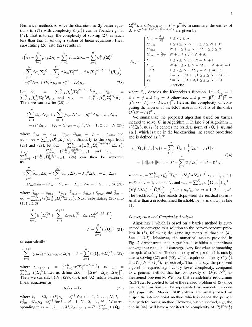
Algorithm 1 The proposed numerical algorithm to solve(6)
Initinalization: Qk := Ink, ψ := 1, µ1 = µ2 = 1, t := t0,
γ, and tolerance ε > 01: repeat Outer iteration2: repeat inner iteration (centering step)3: Solve (27) to find Σ
(i)k for 1 ≤ k ≤ K and 0 ≤ i ≤
N +M + 1.4: Solve (33) to find ∆ψ and ∆µi.5: Backtracking line search:6: s = 17: while r(Qk + s∆Qk,ψ + s∆ψ, µi +
s∆µi) > (1−αs)r(Qk,ψ, µi) or Qk+s∆Qk 0 do
8: s = βs9: end while
10: Update primal and dual variables: Qk := Qk +s∆Qk; ψ := ψ + s∆ψ, µi := µi + s∆µi
11: until r(Qk,ψ, µi) < ε12: Increase t: t = γt.13: until t is sufficiently large to tolerate the duality gap.
which is higher than that in our proposed algorithm, especiallywhen K is large.
IV. NUMERICAL RESULTS
In this section, we provide numerical examples to illustratethe results of the proposed algorithm. The entry of the channelmatrix from the secondary BS to the kth SU is modeled ascorrelated Rayleigh fading, i.e., Hk = P
1/2k HkR
1/2k where
Hk is a matrix of independent circularly symmetric complexGaussian (CSCG) random variables with zero mean and unitvariance, and Pk ∈ Cnk×nk and Rk ∈ CN×N are thereceive and transmit correlation matrices, respectively. In oursimulation setups, the exponential correlation model is used,where Pk and Rk are generated as [Pk]i,j = r
|i−j|k and
[Rk]i,j = r|i−j|k , respectively [45], [46]. The correlation coef-
ficients rk and rk are given by rk = r×ejφk and rk = r×ejφk ,where r ∈ [0, 1] and φk and φk are i.i.d. and uniformlydistributed over [0, 2π). The channel from the secondary BSto the mth PU is generated as Gm = P
1/2m GmR
1/2m and the
covariance matrices Pm and Rm are generated similarly asdescribed above. The number of antennas at each SU receiveris set to nk = 2 for all k. For simplicity, we further assumethe interference thresholds for all PUs are equal, i.e., Im = I ,for all m, and the resultant power constraint for each antennais Pn = P/N for all n, where P is the total power budget.The SRs are averaged over 10,000 simulation trials. For thepurpose of exposition, the results in Figs. 3-7 are shown withr = 0, i.e., uncorrelated Rayleigh fading.
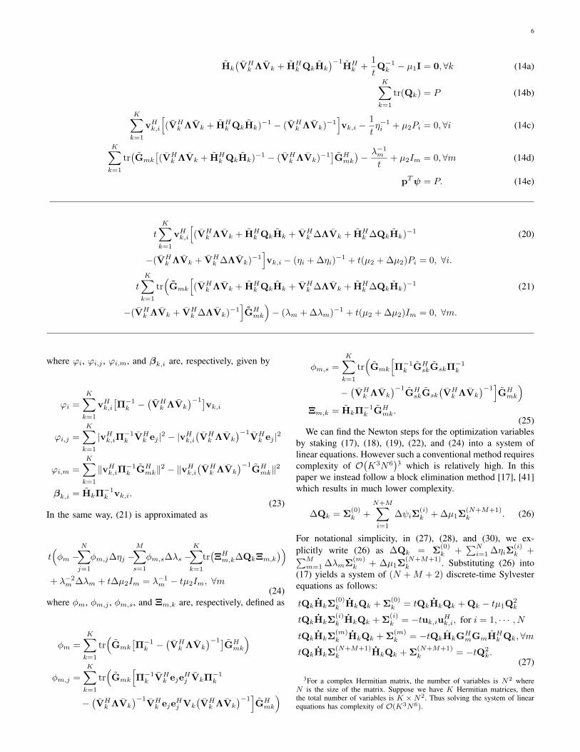
In Fig. 2 we show the convergence rate of the proposedalgorithm for the simulation settings given in the caption.In particular, we plot the convergence rate of the proposedbarrier method for different numbers of transmit antennasat the secondary BS in Fig. 2(a), and for different numbersof PUs in Fig. 2(b). The initial values for the primal and
1 5 10 15 20 25 30 35 4010−7
10−6
10−5
10−4
10−3
10−2
10−1
100
101
Number of iterations
Res
idua
lerr
or
N = 6N = 10N = 14
(a) Convergence results of Algorithm 1 for different numbers oftransmit antennas at the secondary BS. The number of PUs isM = 1.
1 5 10 15 20 25 30 35 4010−7
10−6
10−5
10−4
10−3
10−2
10−1
100
101
Number of iterations
Res
idua
lerr
or
M = 1M = 2M = 3
(b) Convergence results of Algorithm 1 for different numbers ofPUs. The number of transmit antennas is N = 10.
Figure 2: Convergence results of the proposed algorithm (a) fordifferent numbers of transmit antennas at the secondary BS,and (b) for different numbers of PUs. Each curve is obtainedfor one channel realization. The parameters of Algorithm 1are as follows. The tolerance is set to ε = 10−5. The barrierparameters γ and t0 are set to 1 and 50, respectively. Thebacktracking line search parameters in Algorithm 1 are set toα = 0.01 and β = 0.5. In this example, we set the networkparameters as K = 2, nk = 2,∀k, nm = 2,∀m,P = 10 dB,and I = 5 dB.
dual variables in Algorithm 1 are randomly generated. Wecan see that Algorithm 1 shows a very fast convergence ratewhen it is approaching the optimal solution. We note that thisconvergence result can be expected for an algorithm based onNewton’s method. We can also see that its convergence rateis slightly sensitive to the network configurations.
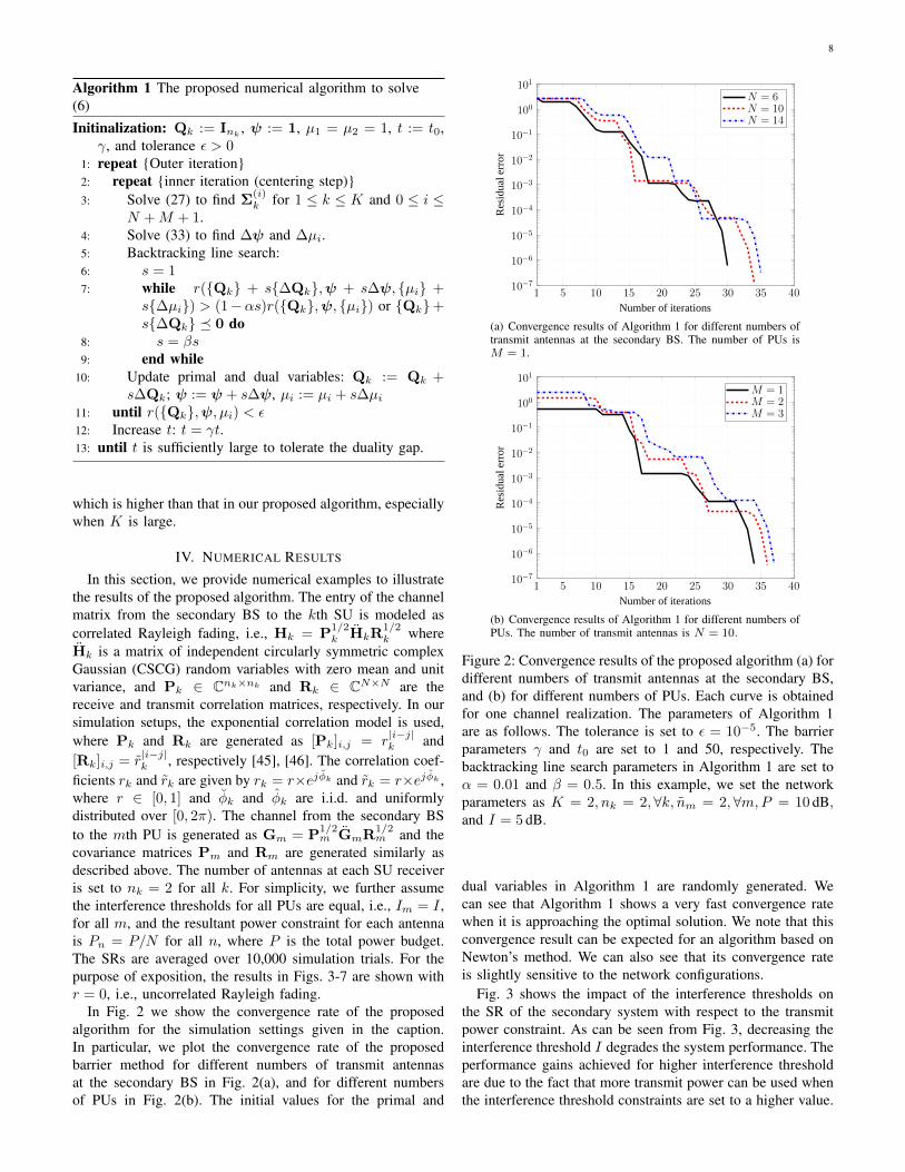
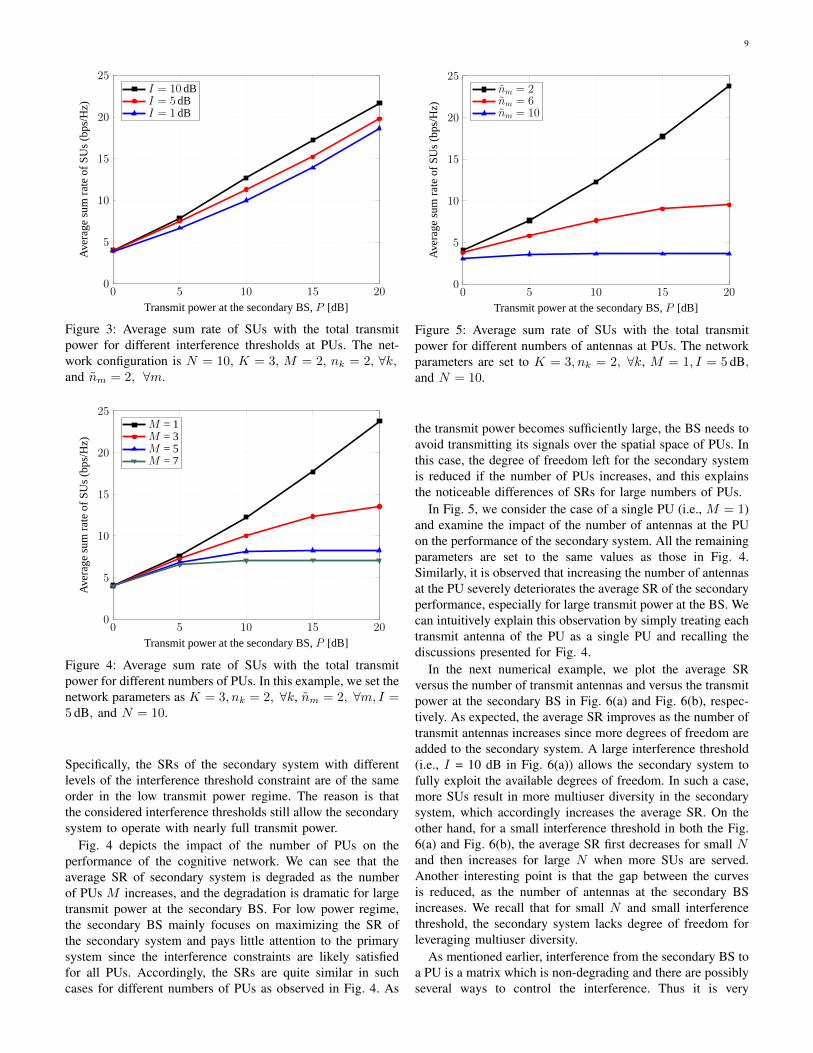
Fig. 3 shows the impact of the interference thresholds onthe SR of the secondary system with respect to the transmitpower constraint. As can be seen from Fig. 3, decreasing theinterference threshold I degrades the system performance. Theperformance gains achieved for higher interference thresholdare due to the fact that more transmit power can be used whenthe interference threshold constraints are set to a higher value.
9
0 5 10 15 200
5
10
15
20
25
Transmit power at the secondary BS, P [dB]
Ave
rage
sum
rate
ofS
Us
(bps
/Hz)
I = 10 dBI = 5 dBI = 1 dB
Figure 3: Average sum rate of SUs with the total transmitpower for different interference thresholds at PUs. The net-work configuration is N = 10, K = 3, M = 2, nk = 2, ∀k,and nm = 2, ∀m.
0 5 10 15 200
5
10
15
20
25
Transmit power at the secondary BS, P [dB]
Ave
rage
sum
rate
ofS
Us
(bps
/Hz)
M = 1M = 3M = 5M = 7
Figure 4: Average sum rate of SUs with the total transmitpower for different numbers of PUs. In this example, we set thenetwork parameters as K = 3, nk = 2, ∀k, nm = 2, ∀m, I =5 dB, and N = 10.
Specifically, the SRs of the secondary system with differentlevels of the interference threshold constraint are of the sameorder in the low transmit power regime. The reason is thatthe considered interference thresholds still allow the secondarysystem to operate with nearly full transmit power.
Fig. 4 depicts the impact of the number of PUs on theperformance of the cognitive network. We can see that theaverage SR of secondary system is degraded as the numberof PUs M increases, and the degradation is dramatic for largetransmit power at the secondary BS. For low power regime,the secondary BS mainly focuses on maximizing the SR ofthe secondary system and pays little attention to the primarysystem since the interference constraints are likely satisfiedfor all PUs. Accordingly, the SRs are quite similar in suchcases for different numbers of PUs as observed in Fig. 4. As
0 5 10 15 200
5
10
15
20
25
Transmit power at the secondary BS, P [dB]
Ave
rage
sum
rate
ofS
Us
(bps
/Hz)
nm = 2nm = 6nm = 10
Figure 5: Average sum rate of SUs with the total transmitpower for different numbers of antennas at PUs. The networkparameters are set to K = 3, nk = 2, ∀k, M = 1, I = 5 dB,and N = 10.
the transmit power becomes sufficiently large, the BS needs toavoid transmitting its signals over the spatial space of PUs. Inthis case, the degree of freedom left for the secondary systemis reduced if the number of PUs increases, and this explainsthe noticeable differences of SRs for large numbers of PUs.
In Fig. 5, we consider the case of a single PU (i.e., M = 1)and examine the impact of the number of antennas at the PUon the performance of the secondary system. All the remainingparameters are set to the same values as those in Fig. 4.Similarly, it is observed that increasing the number of antennasat the PU severely deteriorates the average SR of the secondaryperformance, especially for large transmit power at the BS. Wecan intuitively explain this observation by simply treating eachtransmit antenna of the PU as a single PU and recalling thediscussions presented for Fig. 4.
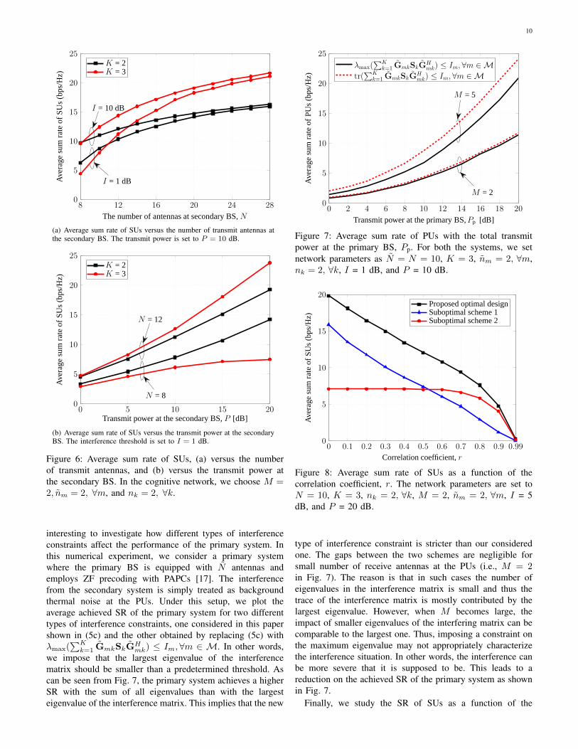
In the next numerical example, we plot the average SRversus the number of transmit antennas and versus the transmitpower at the secondary BS in Fig. 6(a) and Fig. 6(b), respec-tively. As expected, the average SR improves as the number oftransmit antennas increases since more degrees of freedom areadded to the secondary system. A large interference threshold(i.e., I = 10 dB in Fig. 6(a)) allows the secondary system tofully exploit the available degrees of freedom. In such a case,more SUs result in more multiuser diversity in the secondarysystem, which accordingly increases the average SR. On theother hand, for a small interference threshold in both the Fig.6(a) and Fig. 6(b), the average SR first decreases for small Nand then increases for large N when more SUs are served.Another interesting point is that the gap between the curvesis reduced, as the number of antennas at the secondary BSincreases. We recall that for small N and small interferencethreshold, the secondary system lacks degree of freedom forleveraging multiuser diversity.
As mentioned earlier, interference from the secondary BS toa PU is a matrix which is non-degrading and there are possiblyseveral ways to control the interference. Thus it is very
10
8 12 16 20 24 280
5
10
15
20
25
The number of antennas at secondary BS, N
Ave
rage
sum
rate
ofS
Us
(bps
/Hz)
K = 2K = 3
I = 1 dB
I = 10 dB
(a) Average sum rate of SUs versus the number of transmit antennas atthe secondary BS. The transmit power is set to P = 10 dB.
0 5 10 15 200
5
10
15
20
25
Transmit power at the secondary BS, P [dB]
Ave
rage
sum
rate
ofS
Us
(bps
/Hz)
K = 2K = 3
N = 8
N = 12
(b) Average sum rate of SUs versus the transmit power at the secondaryBS. The interference threshold is set to I = 1 dB.
Figure 6: Average sum rate of SUs, (a) versus the numberof transmit antennas, and (b) versus the transmit power atthe secondary BS. In the cognitive network, we choose M =2, nm = 2, ∀m, and nk = 2, ∀k.
interesting to investigate how different types of interferenceconstraints affect the performance of the primary system. Inthis numerical experiment, we consider a primary systemwhere the primary BS is equipped with N antennas andemploys ZF precoding with PAPCs [17]. The interferencefrom the secondary system is simply treated as backgroundthermal noise at the PUs. Under this setup, we plot theaverage achieved SR of the primary system for two differenttypes of interference constraints, one considered in this papershown in (5c) and the other obtained by replacing (5c) withλmax(
∑Kk=1 GmkSkG
Hmk) ≤ Im,∀m ∈ M. In other words,
we impose that the largest eigenvalue of the interferencematrix should be smaller than a predetermined threshold. Ascan be seen from Fig. 7, the primary system achieves a higherSR with the sum of all eigenvalues than with the largesteigenvalue of the interference matrix. This implies that the new
0 2 4 6 8 10 12 14 16 18 200
5
10
15
20
25
Transmit power at the primary BS,Pp [dB]
Ave
rage
sum
rate
ofP
Us
(bps
/Hz)
λmax(∑K
k=1 GmkSkGHmk) ≤ Im, ∀m ∈ M
tr(∑K
k=1 GmkSkGHmk) ≤ Im, ∀m ∈ M
M = 2
M = 5
Figure 7: Average sum rate of PUs with the total transmitpower at the primary BS, Pp. For both the systems, we setnetwork parameters as N = N = 10, K = 3, nm = 2, ∀m,nk = 2, ∀k, I = 1 dB, and P = 10 dB.
0 0.1 0.2 0.3 0.4 0.5 0.6 0.7 0.8 0.9 0.990
5
10
15
20
Correlation coefficient,r
Ave
rage
sum
rate
ofS
Us
(bps
/Hz) Proposed optimal design
Suboptimal scheme 1Suboptimal scheme 2
Figure 8: Average sum rate of SUs as a function of thecorrelation coefficient, r. The network parameters are set toN = 10, K = 3, nk = 2, ∀k, M = 2, nm = 2, ∀m, I = 5dB, and P = 20 dB.
type of interference constraint is stricter than our consideredone. The gaps between the two schemes are negligible forsmall number of receive antennas at the PUs (i.e., M = 2in Fig. 7). The reason is that in such cases the number ofeigenvalues in the interference matrix is small and thus thetrace of the interference matrix is mostly contributed by thelargest eigenvalue. However, when M becomes large, theimpact of smaller eigenvalues of the interfering matrix can becomparable to the largest one. Thus, imposing a constraint onthe maximum eigenvalue may not appropriately characterizethe interference situation. In other words, the interference canbe more severe that it is supposed to be. This leads to areduction on the achieved SR of the primary system as shownin Fig. 7.
Finally, we study the SR of SUs as a function of the
11
correlation coefficient r in Fig. 8. In particular, we comparethe performance of the proposed design with that of two sub-optimal schemes. For suboptimal scheme 1, the ZF precodingat the secondary BS is chosen to eliminate the interference atboth SUs and PUs. For suboptimal scheme 2, the ZF precodingfor the kth SU is given by Tk = VkVkΦ
1/2k where Vk
contains the nk singular vectors of Hk, i.e., it comes froma compact SVD of Hk: Hk = UkDkV
Hk , and Φk ∈ Cnk×nk
is the solution of (5) [17]. The results show that the SRof all the schemes decreases as the correlation coefficientincreases. This is because a high correlation coefficient reducesthe spatial diversity of the secondary system. Importantly, theproposed design shows superior performance compared to theothers. Another interesting observation is that, in the strongcorrelation regime, the sum rate of the suboptimal scheme2 is larger than that of the suboptimal scheme 1 and viceversa in the weak correlation regime. The reason is that as thespatial correlation at the transmitter and receiver is stronger,the channels become more directional and thus interferenceisolation can be achieved physically. Accordingly, the effectof the secondary system on the primary one will be small.Consequently, the suboptimal scheme 2 has more degreesof freedom when designing the precoders for the secondarysystem as it does not force those precoders to be in the nullspace of the PU channels.
V. CONCLUSIONS
In this paper, we have considered the sum rate maximizationproblem for downlink transmission of MIMO CR networks inthe presence of multiple SUs and PUs. The design problemis subject to per-antenna power constraints at the secondaryBS and interference constraints at the PUs. Adopting ZFprecoding technique and using a rank relaxation method whichis shown to be tight, we have transformed the problem ofSR maximization into the one of finding a saddle point ofa convex-concave program. Then a computationally efficientalgorithm has been proposed based on a barrier method tosolve the resulting convex-concave problem, exploiting itsspecial properties. The proposed algorithm was numericallyshown to have a superlinear convergence behavior which isalmost independent of the problem size. Through numericalexperiments, we have illustrated how the performances of thesecondary and the primary systems vary with the type of theinterference constraints considered in the paper. In particular,we have shown that the performance of the secondary systemdegrades significantly and reaches a saturated value wheneither the number of primary users or the number of antennasat the primary user is large. Also, we have discussed differentways of controlling amount of the interference caused by thesecondary system. Specifically, we have concluded that usingthe trace of the interference matrix may reflect the interferencesituation better, compared to using the largest eigenvalue.
APPENDIXPROOF OF THEOREM 1
To prove Theorem 1, we will follow the same steps asthose in [16] but customize them to our considered problem.
Particularly we show that (6) is the dual problem of the relaxedproblem of (5). Let us start by writing the partial Lagrangianfunction of the relaxed problem of (5) as
L (Sk, ηn, λm) =
K∑k=1
log |I + HkSkHHk |
+
N∑n=1
ηn(Pn −
K∑k=1
tr(SkB
(n)k
))+
M∑m=1
λm(Im − tr
(SkGmk
))(35)
where B(n)k , DH
k Dk, Dk = [0Tn−1 1 0TN−n]Vk andGmk , GH
mkGmk. ηn and λm are Lagrangian mul-tipliers corresponding to the constraints in (5b) and (5c),respectively. From the dual problem, the dual objective of (5)is given by
D(ηn, λm) = maxSk0
L (Sk, ηn, λm) . (36)
To solve the maximization in (36) for a given set of Lagrangianmultipliers (ηn, λm), we first rewrite the Lagrangianfunction as
L (Sk,η,λ) =
K∑
k=1
log |I + HkSkHHk |
−K∑
k=1
tr(SkΩk
)+ pTη + I
Tλ
(37)
where Ωk ,∑Nn=1 ηnB
(n)k +
∑Mm=1 λmGmk =
VHk
(diag(η) +
∑Mm=1 λmGH
mGm
)Vk, p =
[P1, P2, · · · , PN ]T , η = [η1, η2, · · · , ηN ]T , I =[I1, I2, · · · , IM ]T , and λ = [λ1, λ2, · · · , λM ]T . SinceΩk is invertible4, let Sk = Ω
1/2k SkΩ
1/2k . The maximization
in (37) is rewritten as
L(Sk,η,λ
)=
K∑
k=1
log |I + HkΩ−1/2k SkΩ
−1/2k HH
k |
−K∑
k=1
tr(Sk)
+ pTη + ITλ.
(38)
To compute the dual objective, let UkDkVHk be a SVD of
HkΩ−1/2k where Dk is square and diagonal. Then, we can
apply a result in [38, Appendix A] to find D(η,λ) as
D(η,λ) = maxQk0
K∑
k=1
log |I + Ω−1/2k HH
k QkHkΩ−1/2k |
−K∑
k=1
tr(Qk
)+ pTη + I
Tλ (39)
where the relationship between Sk and Qk is given by
Sk = VkUHk QkUkV
Hk
Qk = UkVHk SkVkU
Hk .
(40)
4It implies that ηn or λm must be positive. This is because of allpower at the secondary BS should be used up or the interference constraintshould be met at the optimum, i.e., η∗n > 0 or λ∗m > 0.

12
From (39) we can further write D(η,λ) as
D(ψ)= maxQk0
K∑
k=1
log |I + Ω−1/2k HH
k QkHkΩ−1/2k |
−K∑
k=1
tr(Qk
)+ pTψ
= maxQk0
K∑
k=1
log|VH
k ΛVk + HHk QkHk|
|VHk ΛVk|
−K∑
k=1
tr(Qk
)+ pTψ (41)
where Λ = diag(η) +∑Mm=1 λmGH
mGm, p = [pT IT
]T ,and ψ = [ηT λT ]T .
Now the dual problem of (5) is given by
minD(ψ)
s. t.ψ ≥ 0.(42)
or equivalently
minψ≥0
maxQk0
∑Kk=1 log
|VHk ΛVk+HH
k QkHk||VH
k ΛVk|
−∑Kk=1 tr
(Qk
)+ pTψ
(43)
To arrive at a minimax program given in (6), we introduceanother optimization variable ϑ ≥ 0 and rewrite (43) as
minψ≥0
maxϑ≥0,Qk0
∑Kk=1 log
|VHk ΛVk+HH
k QkHk||VH
k ΛVk|
−ϑP + pTψ
s. t.∑Kk=1 tr
(Qk
)≤ ϑP.
(44)
It is easy to see that (44) is equivalent to (43) since theinequality (use subequation environment and give a label tothe trace(·) constraint) in (44) must hold with equality atoptimality; otherwise we can scale down ϑ to achieve a strictlylarger objective. Next we make a change of variables as
η = η/ϑ
λ = λ/ϑ
Qk = Qk/ϑ.
(45)
and define
ψ = ψ/ϑ = [ηT λT
]T
Λ = Λ/ϑ = diag(η) +
M∑
m=1
λmGHmGm.
(46)
We now consider ψ and Qk as new optimization variables.Then, (44) can be equivalently expressed as
minψ≥0
maxϑ≥0,Qk0
∑Kk=1 log
|VHk ΛVk+HH
k QkHk||VH
k ΛVk|
+ϑ(pT ψ − P )
s. t.∑Kk=1 tr
(Qk
)≤ P.
(47)
Clearly, the optimal dual variable ϑ∗ can be obtained byconsidering the minimization of (47) over ψ. Hence, (47) is
the dual of the following problem:
minψ≥0
maxϑ≥0,Qk0
∑Kk=1 log
|VHk ΛVk+HH
k QkHk||VH
k ΛVk|
s. t.∑Kk=1 tr
(Qk
)≤ P
pT ψ ≤ P.(48)
Finally, putting (40), (45), (48) and Sk = Ω−1/2k SkΩ
−1/2k
together finalizes the proof.We now show how Theorem 1 can be modified to include
a SPC constraint which is written as∑Kk=1 tr(TkT
Hk ) ≤ P ,
where P is the total transmit power at the secondary BS. Byfollowing the same steps from (35) to (48), we can arrive at thesame convex-concave program as the one in Theorem 1, exceptthat Λ, ψ, and p are changed to Λ = ηI+
∑Mm=1 λmGH
mGm,ψ = [η λT ]T , and p = [P I
T]T , respectively. Conse-
quently, Algorithm 1 can be applied to handle this case.
REFERENCES
[1] Spectrum Policy Task Force, Report of the spectrum efficiency workinggroup Fed. Commun. Commiss., 2002, Tech. Rep. ET Docket-135.
[2] J. Mitola III and G. Q. Maguire, “Cognitive radios: Making softwareradios more personal,” IEEE Personal Commun., vol. 6, no. 4, pp. 13–18, Aug. 1999.
[3] S. Haykin, “Cognitive radio: Brain-empowered wireless communica-tions,” IEEE J. Select. Areas Commun., vol. 23, no. 2, pp. 201–202, Feb.2005.
[4] X. Gan and B. Chen, “A novel sensing scheme for dynamic multichannelaccess,” IEEE Trans. Veh. Technol., vol. 61, no. 1, pp. 208–221, Jan.2012.
[5] E. C. Y. Peh, Y.-C. Liang, Y. L. Guan, and Y. Zeng, “Optimization ofcooperative sensing in cognitive radio networks: A sensing-throughputtradeoff view,” IEEE Trans. Veh. Technol., vol. 58, no. 9, pp. 5294–5299,Nov. 2009.
[6] D. He, Y. Lin, C. He, and L. Jiang, “A novel spectrum-sensing techniquein cognitive radio based on stochastic resonance,” IEEE Trans. Veh.Technol., vol. 59, no. 4, pp. 1680–1688, May 2010.
[7] J. T. Wang, “Maximum-minimum throughput for MIMO system incognitive radio network,” IEEE Trans. Veh. Technol., vol. 63, no. 1,pp. 217–224, Jan. 2014.
[8] S. Hua, H. Liu, X. Zhuo, M. Wu, and S. S. Panwar, “Exploiting multipleantennas in cooperative cognitive radio networks,” IEEE Trans. Veh.Technol., vol. 63, no. 7, pp. 3318–3330, Sept. 2014.
[9] L. Zhang, Y. Liang, and Y. Xin, “Joint beamforming and power allocationfor multiple access channels in cognitive radio networks,” IEEE J. Select.Areas Commun., vol. 26, no. 1, pp. 38–51, Jan. 2008.
[10] F. A. Khan, C. Masouros, and T. Ratnarajah, “Interference-driven linearprecoding in multiuser MISO downlink cognitive radio network,” IEEETrans. Veh. Technol., vol. 61, no. 6, pp. 2531–2543, July 2012.
[11] R. Zhang and Y.-C. Liang, “Exploiting multi-antennas for opportunisticspectrum sharing in cognitive radio networks,” IEEE J. Select. TopicsSignal Process., vol. 2, no. 1, pp. 88–102, Feb. 2008.
[12] H. Sun, A. Nallanathan, S. Cui, and C.-X. Wang, “Cooperative widebandspectrum sensing over fading channels,” IEEE Trans. Veh. Technol., DOI10.1109/TVT.2015.2407700, Feb. 2015.
[13] E. A. Gharavol, Y.-C. Liang, and K. Mouthaan, “Robust downlinkbeamforming in multiuser MISO cognitive radio networks with imperfectchannel-state information,” IEEE Trans. Veh. Technol., vol. 59, no. 6,pp. 2852–2860, July 2010.
[14] G. Caire and S. Shamai, “On the achievable throughput of a multi-antenna Gaussian broadcast channel,” IEEE Trans. Inform. Theory,vol. 49, no. 7, pp. 1691–1706, July 2003.
[15] A. Dabbagh and D. Love, “Precoding for multiple antenna Gaussianbroadcast channels with successive zero-forcing,” IEEE Trans. SignalProcess., vol. 55, no. 7, pp. 3837–3850, July 2007.
[16] L.-N. Tran, M. Juntti, M. Bengtsson, and B. Ottersten, “Beamformerdesigns for MISO broadcast channels with zero-forcing dirty papercoding,” IEEE Trans. Wireless Commun., vol. 12, no. 3, pp. 1173–1185,Mar. 2013.

13
[17] L.-N. Tran, M. Juntti, M. Bengtsson, and B. Ottersten, “Weightedsum rate maximization for MIMO broadcast channels using dirty papercoding and zero-forcing methods,” IEEE Trans. Commun., vol. 61, no. 6,pp. 2362–2373, June 2013.
[18] R. Zhang, “Cooperative multi-cell block diagonalization with per-base-station power constraints,” IEEE J. Select. Areas Commun., vol. 28, no. 9,pp. 1435–1445, Dec. 2010.
[19] A. Ghasemi and E. S. Sousa, “Fundamental limits of spectrum-sharingin fading environments,” IEEE Trans. Wireless Commun., vol. 6, no. 2,pp. 649–658, Feb. 2007.
[20] J. Huang, R. Berry, and M. L. Honig, “Auction-based spectrum sharing,”Mobile Networks Applicat. J. (MONET), vol. 11, no. 3, pp. 405–418, June2006.
[21] Y. Xing, C. N. Mathur, M. A. Haleem, R. Chandramouli, and K. P. Sub-balakshmi, “Dynamic spectrum access with QoS and interference temper-ature constraints,” IEEE Trans. Mobile Comput., vol. 6, no. 4, pp. 423–433, Apr. 2007.
[22] A. Tajer, N. Prasad, and X. Wang, “Beamforming and rate allocation inMISO cognitive radio networks,” IEEE Trans. Signal Process., vol. 58,no. 1, pp. 362–377, Jan. 2010.
[23] S. A. Jafar and S. Srinivasa, “Capacity limits of cognitive radio with dis-tributed and dynamic spectral activity,” IEEE J. Select. Areas Commun.,vol. 25, no. 3, pp. 529–537, Apr. 2007.
[24] R. Zhang, “On peak versus average interference power constraintsfor protecting primary users in cognitive radio networks,” IEEE Trans.Wireless Commun., vol. 8, no. 4, pp. 1128–1138, May 2009.
[25] S. Stotas and A. Nallanathan, “On the throughput and spectrum sensingenhancement of opportunistic spectrum access cognitive radio networks,”IEEE Trans. Wireless Commun., vol. 11, no. 1, pp. 97–107, Jan. 2012.
[26] F. Rezaei and A. Tadaion, “Sum rate improvement in cognitive ra-dio through interference alignment” IEEE Trans. Veh. Technol., DOI:10.1109/TVT.2015.2392152, Jan. 2015.
[27] T. Luan, F. Gao, X.-D. Zhang, J. C. F. Li, and M. Lei, “Rate max-imization and beamforming design for relay-aided multiuser cognitivenetworks,” IEEE Trans. Veh. Technol., vol. 61, no. 4 Jan. 2015.
[28] L. Zhang, Y. Xin, and Y. Liang, “Weighted sum rate optimizationfor cognitive radio MIMO broadcast channels,” IEEE Trans. WirelessCommun., vol. 8, no. 6, pp. 2950–2959, June 2009.
[29] L. Gallo, F. Negro, I. Ghauri, and D. T. M. Slock, “Weighted sumrate maximization in the underlay cognitive MISO interference channel,”in Proc. IEEE Inter. Symposium on Personal, Indoor and Mobile RadioCommun. (PIMRC), pp. 661–665, Toronto, Canada, Sept. 2011.
[30] S. Kim and G. B. Giannakis, “Optimal resource allocation for MIMOad hoc cognitive radio networks,” IEEE Trans. Inform. Theory, vol. 57,no. 5, pp. 3117–3131, May 2011.
[31] K. Jitvanichphaibool, Y.-C. Liang, and R. Zhang, “Beamforming andpower control for multi-antenna cognitive two-way relaying,” in Proc.IEEE Wireless Commun. and Networking Conf. (WCNC), pp. 1–6, Bu-dapest, Hungary, Apr. 2009.
[32] Y. Y. He and S. Dey, “Sum rate maximization for cognitive MISObroadcast channels: Beamforming design and large systems analysis,”IEEE Trans. Wireless Commun., vol. 13, no. 5, pp. 2383–2401, May2014.
[33] L. Zheng and C. W. Tan, “Maximizing sum rates in cognitive radionetworks: Convex relaxation and global optimization algorithms,” IEEEJ. Select. Areas in Commun., vol. 32, no. 3, pp. 667–680, Mar. 2014.
[34] I.-W. Lai, L. Zheng, C. H. Lee, and C. W. Tan, “Beamforming dualityand algorithms for weighted sum rate maximization in cognitive radionetworks,” IEEE J. Select. Areas Commun., vol. 33, no. 5, pp. 832–847,May 2015.
[35] H. Weingarten, Y. Steinberg, and S. Shamai, “The capacity region of theGaussian multiple-input multiple-output broadcast channel,” IEEE Trans.Inform. Theory, vol. 52, no. 9, pp. 3936–3964, Sept. 2006.
[36] J. F. Sturm, “Using SeDuMi 1.02, a MATLAB toolbox for optimizationover symmetric cones,” Optimiz. Methods and Softw., vol. 11–12, pp. 625–653, Sept. 1999.
[37] K. C. Toh, M. J. Todd, and R. H. Tutuncu, “SDPT3 a Matlab softwarepackage for semidefinite programming, version 1.3,” Optimiz. Methodsand Softw., vol. 11, pp. 545–581, Jan. 1999.
[38] S. Vishwanath, N. Jindal, and A. Goldsmith, “Duality, achievable ratesand sum rate capacity of Gaussian MIMO broadcast channels,” IEEETrans. Inform. Theory, vol. 49, no. 10, pp. 2658–2668, Oct. 2003.
[39] J. Zhang and M. C. Gursoy, “Collaborative relay beamforming forsecrecy,” in Proc. IEEE Inter. Conf. Commun. (ICC), pp. 1–5, Cape Town,South Africa, May 2010.
[40] W. Yu and T. Lan, “Transmitter optimization for the multi-antenna down-link with per-antenna power constraints,” IEEE Trans. Signal Process.,vol. 55, no. 6, pp. 2646–2660, June 2007.
[41] S. Boyd and L. Vandenberghe, Convex Optimization. Cambridge Univ.Press, UK, 2007.
[42] N. J. Higham, Accuracy and Stability of Numerical Algorithms, 2ndedition. Society for Industrial and Applied Mathematics, 2002.
[43] http://epubs.siam.org/doi/book/10.1137/1.9780898718829.[44] http://epubs.siam.org/doi/abs/10.1137/0806020.[45] S. L. Loyka, “Channel capacity of MIMO architecture using the expo-
nential correlation matrix,” IEEE Commun. Lett. vol. 5, no. 9, pp. 369–371, Sept. 2001.
[46] L.-N. Tran, M. Bengtsson, and B. Ottersten, “Iterative precoder designand user scheduling for block-diagonalized systems,” IEEE Trans. SignalProcess., vol. 60, no. 7, pp. 3726–3739, July 2012.
Van-Dinh Nguyen received his B.S. degree inTelecommunications from Ho Chi Minh City Uni-versity of Technology, Vietnam, in 2012, and hisM.S. degree in Electronic Engineering from SoongsilUniversity, Seoul, Korea, in 2015. He was a visitingstudent at Queen’s University Belfast, UK (June-July2015 and August 2016). Currently, he is pursuing hisPh.D. degree in Electronic Engineering at SoongsilUniversity, Seoul, Korea. His research interests in-clude wireless communications, information theory,massive MIMO, stochastic geometry, physical layer
security, energy harvesting, cooperative communications, and cognitive radio.
Le-Nam Tran (M’10) received the B.S. degree inelectrical engineering from Ho Chi Minh City Uni-versity of Technology, Ho Chi Minh City, Vietnam,in 2003 and the M.S. and Ph.D. degrees in radio en-gineering from Kyung Hee University, Seoul, Korea,in 2006 and 2009, respectively. In 2009, he joinedthe Department of Electrical Engineering, KyungHee University, as a Lecturer. From 2010 to 2014, hehad held postdoc positions at the Signal ProcessingLaboratory, ACCESS Linnaeus Centre, KTH RoyalInstitute of Technology, Stockholm, Sweden (2010-
2011), and at Centre for Wireless Communications and the Department ofCommunications Engineering, University of Oulu, Finland (2011-2014). Hehas been a lecturer at the Department of Electronic Engineering, MaynoothUniversity, Co. Kildare, Ireland since Sep. 2014. His current research interestsinclude multiuser MIMO systems, energy-efficient communications, full-duplex transmission, and applications of optimization techniques.

14
Trung Q. Duong (S’05–M’12–SM’13) received hisPh.D. degree in Telecommunications Systems fromBlekinge Institute of Technology (BTH), Sweden in2012. Since 2013, he has joined Queen’s UniversityBelfast, UK as a Lecturer (Assistant Professor). Hiscurrent research interests include physical layer se-curity, energy-harvesting communications, cognitiverelay networks. He is the author or co-author of morethan 200 technical papers published in scientificjournals and presented at international conferences.
Dr. Duong currently serves as an Editor for theIEEE TRANSACTIONS ON COMMUNICATIONS, IEEE COMMUNICATIONSLETTERS, IET COMMUNICATIONS, WILEY TRANSACTIONS ON EMERGINGTELECOMMUNICATIONS TECHNOLOGIES, and ELECTRONICS LETTERS. Hehas also served as the Guest Editor of the special issue on some majorjournals including IEEE JOURNAL IN SELECTED AREAS ON COMMUNI-CATIONS, IET COMMUNICATIONS, IEEE WIRELESS COMMUNICATIONSMAGAZINE, IEEE COMMUNICATIONS MAGAZINE, EURASIP JOURNALON WIRELESS COMMUNICATIONS AND NETWORKING, EURASIP JOUR-NAL ON ADVANCES SIGNAL PROCESSING. He was awarded the Best PaperAward at the IEEE Vehicular Technology Conference (VTC-Spring) in 2013,IEEE International Conference on Communications (ICC) 2014. He is therecipient of prestigious Royal Academy of Engineering Research Fellowship(2015-2020).
Oh-Soon Shin (S’00-M’10) received his B.S., M.S.,and Ph.D. degrees in Electrical Engineering andComputer Science from Seoul National University,Seoul, Korea, in 1998, 2000, and 2004, respectively.From 2004 to 2005, he was with the Division of En-gineering and Applied Sciences, Harvard University,MA, USA, as a Postdoctoral Fellow. From 2006 to2007, he was a Senior Engineer at Samsung Elec-tronics, Suwon, Korea. In September 2007, he joinedthe School of Electronic Engineering, Soongsil Uni-versity, Seoul, Korea, where he is currently an Asso-
ciate Professor. His research interests include communication theory, wirelesscommunication systems, and signal processing for communication.
Ronan Farrell (S’89-M’93) received the PhD de-gree from the Department of Electrical and Elec-tronic Engineering, University College Dublin, in1998. In 2001 he joined Maynooth University asa lecturer, promoted to Senior Lecturer in 2010.In 2008 he was appointed Director for the CallanInstitute for Applied ICT, and in 2012 was namedHead of the Department of Electronic Engineering.In 2004, he became an SFI theme leader for radiofrequency electronics research within the Centrefor Telecommunications Research and later the SFI
supported CONNECT Centre for the Internet of Things. Dr. Farrell haspublished extensively on topics such as software defined radio, RF integratedcircuit design, and radio transceiver architectures.