An efficient, reliable and robust error estimator for elliptic problems in

Applied Numerical Mathematics 61 (2011) 675–695

Contents lists available at ScienceDirect

Applied Numerical Mathematics

www.elsevier.com/locate/apnum

An efficient, reliable and robust error estimator for elliptic problems in R3

Michael Holst a, Jeffrey S. Ovall b,∗, Ryan Szypowski a

a Mathematics Department, University of California, San Diego, United Statesb Mathematics Department, University of Kentucky, United States

a r t i c l e i n f o a b s t r a c t

Article history:Received 29 July 2010Received in revised form 18 November 2010Accepted 5 January 2011Available online 18 January 2011

Keywords:Finite elementsA posteriori estimatesReliability

In this article, we develop and analyze a hierarchical-type error estimator for a generalclass of second-order linear elliptic boundary value problems in bounded three-dimensionaldomains. This type of indicator automatically satisfies a global lower bound inequality,thereby giving efficiency, without regularity assumptions beyond those giving well-posedness of the continuous and discrete problems. The main focus of the paper is then toestablish the reverse reliability result: a global upper bound on the error in terms of theerror estimate (plus an oscillation term), again without additional regularity assumptions.The proof of this inequality depends on a clever choice of the space in which the errorindicator lies and a moment-capturing quasi-interpolation result. We finish the article witha series of numerical experiments to illustrate the behavior predicted by the theoreticalresults.

© 2011 IMACS. Published by Elsevier B.V. All rights reserved.

1. Introduction

Adaptive meshing (local refinement and coarsening) based on a posteriori error estimation is an essential componentof efficient and robust finite element algorithms. To be actually useful in computation, the error estimates should be reli-able (never under-estimating the error by too much) and efficient (never over-estimating the error by too much). Together,these properties imply the equivalence of the error estimate and the true error. Depending on the type of estimator underconsideration, either reliability or efficiency will be more difficult to prove.

In this article, we develop and analyze a hierarchical-type error estimator for a general class of second-order linearelliptic boundary value problems in bounded three-dimensional domains. Such estimators are based on the computation ofan approximate error function in an auxiliary discrete space. The general principle which guides both our selection of anappropriate auxiliary space and the effectivity-analysis of the resulting error estimate can be summarized as follows. Weare given a variational problem

Find u ∈ H such that B(u, v) = G(v) for all v ∈ H, (1)

where H is a Hilbert space, B is a continuous, bilinear form which satisfies an inf–sup condition, and G is a boundedlinear functional—these are the necessary and sufficient conditions for well-posedness. We choose some finite-dimensionalapproximation space V ⊂ H, in which we compute an approximation u ≈ u as the solution of

Find u ∈ V such that B(u, v) = G(v) for all v ∈ V . (2)

Finally, an approximate error function ε ≈ u − u is computed in a third discrete space W as the solution of

* Corresponding author.E-mail address: [email protected] (J.S. Ovall).

0168-9274/$30.00 © 2011 IMACS. Published by Elsevier B.V. All rights reserved.doi:10.1016/j.apnum.2011.01.002

http://www.ScienceDirect.com/

http://www.elsevier.com/locate/apnum

mailto:[email protected]

http://dx.doi.org/10.1016/j.apnum.2011.01.002

676 M. Holst et al. / Applied Numerical Mathematics 61 (2011) 675–695

Find ε ∈ W such that B(ε, v) = G(v) − B(u, v){= B(u − u, v)

}for all v ∈ W . (3)

For well-posedness on the discrete level, we must again assume that inf–sup conditions hold for B on both V and W . Forconvenience in exposition, we will instead assume coercivity of B on H, which automatically implies well-posedness (1)–(3).

The selection of W is motivated by the following identity: For all v ∈ H, v ∈ V and w ∈ W , we have

B(u − u, v) = B(ε, w) + B(u − u, v − v − w)

= B(ε, w) + [G(v − v − w) − B(u, v − v − w)

]. (4)

The following two criteria motivate the practical selection of W :

1. It should be possible to choose v + w ∈ V ⊕ W , based on v , in such a way that the variational residual, B(u − u, v − v −w) or [G(v − v − w) − B(u, v − v − w)], is “small”, while maintaining norm-comparability of v and w . In the presentwork, v + w is a quasi-interpolant such that certain local moments of v − (v + w) vanish.

2. The cost of computing of ε ∈ W should be provably acceptable within the general adaptive finite element (solve-estimate-mark-refine) framework.

The resulting analysis yields an upper bound on the norm-error of u − u, in terms of the norm of ε and a “residualoscillation” term which will be described in the course of the paper. Some key benefits of this style of analysis are thatit makes no assumptions beyond what is required for well-posedness and practical implementation, and it is completelytransparent what the associated constants do, and do not, depend upon.

We briefly mention some related work. In [7], hierarchical estimators were examined for both two- and three-dimensional problems; the use cubic face-bubbles was considered, but the estimator was based on the solution of localproblems rather than on a global residual. However, the estimator and the analysis in [7] are not easily extended tonon-symmetric problems with convection terms. A more recent work [3] was apparently the first to consider hierarchi-cal estimators for problems with convection. Their focus was on two-dimensional problems; the analysis was significantlydifferent than that appearing here, and its extension to three dimensions appears problematic. The convection-dominatedcase was one of the primary focuses of [3]; the analysis employs a small constant diffusion parameter ε , similar to theconvection–diffusion example appearing later in this article. Related relevant work includes [13] and several references con-tained therein, whereby data oscillation is managed in the analysis, as opposed to residual oscillation used in the analysisin this article.

Outline of the article

The remainder of this paper is structured as follows. In Section 2, we describe the target class of problems, and assemblesome basic mathematical facts and tools. We briefly examine discretizations based on tetrahedral partitions and conformingfinite element subspaces, introduce notation, and subsequently define an error estimator based on the use of piecewisecubic face-bump functions that satisfy a residual equation. We show that this type of indicator automatically satisfies aglobal lower bound inequality thereby giving efficiency, without regularity assumptions beyond those giving well-posednessof the continuous and discrete problems. The main focus of the paper then shifts to establishing the reverse inequality:a global upper bound on the error in terms of the error estimate (plus an oscillation term), again without regularity as-sumptions, thereby giving also reliability. In Section 3, we begin the analysis by developing some basic geometrical identitiesfor conforming discretizations based on tetrahedral partitions. Section 4 contains the main theoretical results of the paper.We begin by stating some quasi-interpolation results, the proofs of which we delay until Section 5. We then establish acollection of scale-invariant inequalities for the residual that are critical for establishing the global upper bound. The mainresult (the global upper bound in Theorem 4.6) is then established. In Section 5, we give the technical proofs of the quasi-interpolant results needed for the main result. In Section 6, we give an analysis of the computational costs of actuallycomputing the error indicator. Through a sequence of spectral equivalence inequalities, we show that the cost to evaluatethe indicator (involving the solution of a linear system) is linear in the number of degrees of freedom. In Section 7, wegive a sequence of numerical experiments to illustrate the behavior predicted by the theoretical results, including: a Poissonproblem on a 3D L-shaped domain, a jump coefficient problem in a cube, a convection–diffusion problem, and a stronglyanisotropic diffusion problem. In Section 8, we reflect on the analysis and results, and consider possible extensions.

2. Model problem and basic theory

Let Ω ⊂ R3 be polyhedral and possibly non-convex, with boundary ∂Ω = ∂ΩD ∪ ∂ΩN —a disjoint union with ∂ΩD

relatively closed. We take H = H1D(Ω) = {u ∈ H1(Ω): u|∂ΩD

= 0}. Let ω ⊂ Ω . We take the standard Sobolev norms andsemi-norms:

‖v‖2k,ω =

∑|α|�k

∥∥Dα v∥∥2

L2(ω), |v|2k,ω =

∑|α|=k

∥∥Dα v∥∥2

L2(ω). (5)

When ω = Ω we omit it from the subscript.

M. Holst et al. / Applied Numerical Mathematics 61 (2011) 675–695 677

We are interested in the problem (1), where

B(u, v) =∫Ω

A∇u · ∇v + (b · ∇u + cu)v dx, (6)

G(v) =∫Ω

f v dx +∫

∂ΩN

gv ds. (7)

We will assume that A ∈ [L∞(Ω)]3×3, b ∈ [L∞(Ω)]3 and c ∈ L∞(Ω) are piecewise-smooth on some polyhedral partitionof Ω , and f ∈ L2(Ω) and g ∈ L2(∂ΩN ). Furthermore, we assume that A is symmetric and positive-definite almost every-where and that there exist constants m, M > 0 such that

m‖u‖21 � B(u, u),

∣∣B(u, v)∣∣ � M‖u‖1‖v‖1. (8)

The coercivity condition (lower bound) is a convenient sufficient for (1) to be well-posed.Given a conforming tetrahedral partition T of Ω , having: tetrahedra T ∈ T , faces F ∈ F , edges E ∈ E and vertices z ∈ V ,

we approximate the solution of (1) and the corresponding error via (1) and (3), respectively, where

V = {v ∈ H ∩ C(Ω): v |T ∈ P1 for every T ∈ T

}, (9)

W = {v ∈ H ∩ C(Ω): v |T ∈ P3 for every T ∈ T and v |E = 0 for every E ∈ E

}. (10)

Here Pk denotes the collection of polynomials of (total) degree no greater than k. We will implicitly assume that T linesup perfectly with any discontinuities in the data. The space V is the standard, conforming, piecewise-linear finite elementspace, and the space W consists of highly-oscillatory (with respect to T ) functions spanned by cubic “face-bump” or “face-bubble” functions. The reasons for our (somewhat non-standard) choice of W will become clear as the error and costanalyses are presented.

The coercivity of B on H implies that problems (2) and (3) are also well-posed. From (3) we automatically get anefficiency bound on the error and error estimate:

m‖ε‖21 � B(ε, ε) = B(u − u, ε) � M‖u − u‖1‖ε‖1, (11)

m

M‖ε‖1 � ‖u − u‖1. (12)

In other words, ‖ε‖1 does not over-estimate the actual error ‖u − u‖1 by too much. The constant m/M in the lower boundtruly is a worst-case scenario, which is unfortunately unavoidable in the analysis without making assumptions beyond thoseneeded for well-posedness. In practice, we see that ε generally provides a slight under-estimate of the true error.

A key objective of this paper is to provide a reliability (upper) estimate to complement (12), in which all quantities areexplicitly computable (or estimable), making no further regularity assumptions on u. Our estimate is of the form:

‖u − u‖1 � K1‖ε‖1 + K2 osc(R, r, T ), (13)

where the oscillation term involves deviations of the element- and face-residuals, R and r, from constants on patches inthe triangulation, and the constants are independent of the f , g, u and the sizes of the elements—though they do dependon their shapes. A detailed description of the oscillation term is given, together with its derivation, in Lemma 4.4. We cansee very clearly in (13) that the only thing that could ever destroy the effectivity of ‖ε‖1 as an estimator of ‖u − u‖1 is ifthe data oscillation is relatively large; but that is something that we can assess and control directly if we choose, because itinvolves no unknown quantities.

Hierarchical error estimators, such as the one we propose, are traditionally analyzed only in the setting in which thebilinear form B is an inner-product, with induced “energy norm” ||| · ||| (cf. [5], [1, Chapter 4]). Such an analysis makes useof a strong Cauchy inequality between the spaces V and W ,∣∣B(v, w)

∣∣ � γ |||v||||||w||| for v ∈ V and w ∈ W , where γ = γ (B, T ) < 1,

as well as a saturation assumption,

infv∈V ⊕W

|||u − v||| � β infv∈V

|||u − v|||, where β = β(B, G, T ) < 1.

From this the following equivalence result between the error and error estimate is obtained

|||ε||| � |||u − u||| � |||ε|||√(1 − γ 2)(1 − β2)

.

A criticism which is sometimes made about such an analysis is that counterexamples to the saturation assumption arereadily constructed for a given mesh and finite-dimensional spaces V and W (cf. [10])—although it could be argued thatsuch cases rarely occur in practical computations. Regardless of how one views this point, such analysis cannot be appliedfor the more general bilinear forms such as those considered here.


Remark 2.1. The traditional analysis referred to above, particularly the saturation assumption, generally leads one to choosean auxiliary space W for which V ⊕ W is a standard approximation space—for example, the piecewise polynomial space ofnext higher degree on the same mesh, or the piecewise polynomial space of the same degree but on a uniformly refinedmesh. This way of thinking might naturally lead one to choose W to be the space of quadratic “edge-bumps” which vanishat every vertex in the mesh, in R

3, so that V ⊕ W is the space of piecewise quadratic functions on the mesh. However, ouranalysis proceeds along different lines, which leads us to choose W as we have.

3. Mesh-related notation and basic results

In this section, we introduce the mesh-related and other notation which will play a role in the analysis given later. Inparticular, we lay out the definitions which are needed to define and analyze the quasi-interpolant whose key propertiesare outlined in Theorem 4.2. Additionally, we collect several basic geometric identities in Lemma 3.2 which will be used invarious arguments throughout the manuscript.

Give a mesh T , we distinguish:

Vertices: Dirichlet V D (z ∈ ∂ΩD ), non-Dirichlet V = V \ V D .Faces: Dirichlet F D (F ⊂ ∂ΩD ), non-Dirichlet F = F \ F D , Neumann FN (F ⊂ ∂ΩN ), interior F I = F \ FN .Non-Dirichlet faces touching z ∈ V : Fz .Tetrahedra touching z ∈ V or F ∈ F : Tz , T F .

For z ∈ V , we define the continuous, piecewise-linear function z by

z(z′) = δzz′ for all z ∈ V. (14)

Also, for any F ∈ F , we define bF = zz′z , where z, z′ and z are the three vertices of F . With these definitions, it is clearthat

V = span{z: z ∈ V}, W = span{bF : F ∈ F }. (15)

The following definitions of patches of elements will also be useful in later analysis:

ωz := supp(z) =⋃

T ∈Tz

T , ωF := supp(bF ) =⋃

T ∈T F

T . (16)

Remark 3.1. We implicitly assume that any vertex in V D will have at least one adjacent vertex in V —so Vz, Fz = ∅. Such anassumption is very natural, and simple to enforce in practice.

Let T be a tetrahedron having: vertices {zk}4k=1, opposite faces {Fk}4

k=1, and outward unit normals to these faces {nk}4k=1.

We denote by θi j the measure of the dihedral angle at the edge shared by faces Fi and F j . We also use k = zk , bk = bFk

and dk = 3|T |/|Fk| = dist(zk, Fk). In the following lemma, we collect various technical facts which will be used, generallywithout reference, in the rest of the paper.

Lemma 3.2. Let i, j,k, l ∈ {1,2,3,4} be distinct. We have

i = 1 − ni

di· (x − zi) = −ni

di· (x − z j) = ∇i · (x − z j) on T , (17)

∫T

p1

q2

r3

s4 = |T |3!p!q!r!s!

(p + q + r + s + 3)! for p,q, r, s ∈ Z�0, (18)

∫Fi

pj

qk

rl = |Fi|2!p!q!r!

(p + q + r + 2)! for p,q, r ∈ Z�0, (19)

∫T

∇bi · ∇b j = 23!|T |

7!(

cos θkl

dkdl− 2 cos θi j

did j

), (20)

∫∇bi · ∇bi = 2

3!|T |7!

4∑k=1

1

d2k

. (21)

T


Finally, for v ∈ H1(T ),

dk

∫Fk

v =∫T

3v + (x − zk) · ∇v. (22)

Throughout this manuscript, the notation |X | will be used to denote the length, area, volume, cardinality or Euclideannorm of X , and the appropriate interpretation will be clear from the context.

Proof. Eqs. (17) are well known, and follow from the facts that such functions are clearly linear and have the correct valuesat the vertices. Eqs. (18)–(19) are also well known—see [20, p. 95], or [15, Theorem A.1], for example. The identities (20)and (21) follow from the definitions of bi , b j and the previous results, with simplifications carried out using forms of“generalized” Laws of Cosines for tetrahedra [2]. These are obtained from the fact that

∑4m=1

nmdm

= −∑4m=1 ∇m = 0, by

equating either one term with the other three, or two terms with the other two, and “squaring” both sides. The final resultis just a direct application of the Divergence Theorem (∇ · (x − zk) = 3). �4. The main results

Before we state our main results, we take the standard definitions for element- and face-residuals, R and r, namely

R |T = f − cu − b · ∇u + ∇ · A∇u, (23)

r|F ={−(A∇u) · nT − (A∇u) · nT ′ , F ∈ FI ,

g − (A∇u) · n, F ∈ FN .(24)

Here, T and T ′ are the two tetrahedra adjacent to F ∈ F I , and nT and nT ′ are their outward unit normals. In order to proveour reliability estimate (13) we first establish the following error equation.

Lemma 4.1. Suppose that vz ∈ V and wz ∈ W for all z ∈ V , and let v = ∑z∈V vz and w = ∑

z∈V wz. Then for any v ∈ H,

B(u − u, v) = B(ε, w) +∑z∈V

∫ωz

R(vz − vz − wz)dV +∑F∈F

∫F

r(v − v − w)dS.

Proof. We have∑

z∈V vz ≡ v , because the z form a partition of unity for Ω . Because of Galerkin orthogonality, B(u −u, vz) = 0, and because of the definition of ε, B(u − u, wz) = B(ε, wz). Using these facts, we deduce

B(u − u, v) =∑z∈V

B(u − u, vz) =∑z∈V

B(u − u, vz − vz − wz) +∑z∈V

B(ε, wz)

= B(ε, w) +∑z∈V

∫ωz

R(vz − vz − wz)dV +∑F∈F

∫F

r(v − v − w)dS,

which completes the proof. �Prudent choices for w and v will allow us to bound B(ε, w) by K (B, T )‖ε‖1|v|1, and yield the oscillation term, osc.

These choices are reflected in the following theorem, whose technical proof is postponed until Section 5.

Theorem 4.2. Let v ∈ H. There is a quasi-interpolant I v = v + w ∈ V ⊕ W , with

• v = ∑z∈V vz and w = ∑

z∈V wz,• supp(vz), supp(wz) ⊂ ωz for z ∈ V ,• supp(vz), supp(wz) ⊂ ωz′ for z ∈ V D , where z′ ∈ V is adjacent to z,

which satisfies the zero-mean properties:∫ωz

(vz − vz − wz) = 0 and

∫F

(v − v − w) = 0 for each F ∈ F .

Furthermore, there are scale-invariant constants C1 , c1z , c2z , c3z and c4F such that

1. |wz|1 � c1z|v|1,ωz , ‖w‖1 � C1|v|1 ,


2. |vz − vz − wz|1 � c2z|v|1,ωz ,3. ‖vz − vz − wz‖0 � c3z Dz|v|1,ωz ,4. ‖v − v − w‖0,F � c4F |F |1/4|v|1,ΩF for each F ∈ F , where ΩF = ωz ∪ ωz′ ∪ ωz′′ , and z, z′, z′′ are the vertices of F .

Here, and following, Dz = diam(ωz).

Remark 4.3. The use of quasi-interpolants of various sorts (e.g. [8,19,21]) in both a priori and a posteriori error estimates hasa long history, though generally not in the context of hierarchical error estimates. Both the choice and the role in analysisof the quasi-interpolant used here share some similarities with that in [14], and it is no coincidence that similar notions ofdata or residual oscillation appear here, as they do in [14] and related works.

Lemma 4.4. Let v ∈ H. There are scale-invariant constants K1 = K1(T , B) and K2 = K2(T ) such that

∣∣B(u − u, v)∣∣ � K1‖ε‖1|v|1 + K2 osc(R, r, T )|v|1,

where

[osc(R, r, T )

]2 =∑z∈V

D2z inf

Rz∈R

‖R − Rz‖20,ωz

+∑F∈F

|F |1/2 infrF ∈R

‖r − rF ‖20,F .

Proof. Using Lemma 4.1 and Theorem 4.2, we see that∣∣B(u − u, v)

∣∣ � M‖ε‖1‖w‖1 +∑z∈V

‖vz − vz − wz‖0,ωz infRz∈R

‖R − Rz‖0,ωz

+∑F∈F

‖v − v − w‖0,F infrF ∈R

‖r − rF ‖0,F

� MC1‖ε‖1|v|1 +∑z∈V

c3z Dz|v|1,ωz infRz∈R

‖R − Rz‖0,ωz

+∑F∈F

c4F |F |1/4|v|1,ΩF infrF ∈R

‖r − rF ‖0,F

� K1‖ε‖1|v|1 + K2 osc(R, r, T )|v|1.The last inequality results from discrete Cauchy–Schwarz inequalities, and the fact that any tetrahedron lies in a (small)finite number of the patches ωz and ΩF , so summing the squares of the semi-norm of v over these patches results in asmall constant multiple of |v|21. �Remark 4.5. It is not uncommon in applications that the diffusion coefficient A ∈ R

3×3 and Neumann data g are piecewise-constant. If we assume this, then the oscillation term simplifies considerably,

[osc(R, r, T )

]2 =∑z∈V

D2z inf

Rz∈R

∥∥( f − cu − b · ∇u) − Rz∥∥2

0,ωz.

In this case, we see that all of the information about the face-residual is “encoded” in ε. If we further have that b = 0, andc, f ∈ H1(Ω), then [osc(R, r, T )]2 �

∑z∈V D4

z . If c and/or f are merely piecewise-smooth, then we will not get these kindsof gains from infRz∈R ‖( f − cu) − Rz‖2

0,ωzwhen z is on an interface across which f and/or c is discontinuous. In such cases,

one could safeguard the error estimation procedure by including the oscillation terms only in such patches ωz , although wegenerally expect that this will be unnecessary.

Based on Lemma 4.4, the following result is immediate.

Theorem 4.6. There are scale-invariant constants K1 = K1(B, T ) and K2 = K2(B, T ) such that

‖u − u‖1 � K1‖ε‖1 + K2 osc(R, r, T ).

Remark 4.7. The constants appearing in Theorem 4.6 are obtained from those in Lemma 4.4 through division by the coerciv-ity constant m. In fact, it is clear from the argument that coercivity is just a convenient sufficient condition for Theorem 4.6,and that an inf–sup condition (which would also have to be assumed for the discrete problems) is what is necessary forthis theorem to hold. In this case, the constants in the bound would be obtained by dividing those in Lemma 4.4 by the(optimal) inf–sup constant.


In practice, the oscillation term is generally ignored both for global error estimates and for local error indicators—this isprecisely what we do in the numerical experiments of Section 7. Of course, it is quite possible to construct examples forwhich the oscillation dominates, or is at least comparable to, the error estimated by ε, but this is something that can oftenbe reliably anticipated from the data itself. At any rate, global estimates and local indicators can be safeguarded by addingon global and local oscillation terms—if only in those areas in which the oscillation is expected to be of similar order (in Dz)to the local interpolation error (cf. Remark 4.5).

5. Proof of Theorem 4.2

In this technical section we prove the existence and key properties of a quasi-interpolant claimed in Theorem 4.2. Thefollowing definition will be convenient for some of the lemmas and theorems below. For F ∈ F , ωF consists of one (in thecase F ∈ FN ) or two (in the case F ∈ F I ) tetrahedra adjacent to F . In the first case, calling the adjacent tetrahedron T , wedefine dF = x − zF T on ωF , where zF T is the vertex of T opposite F . In the second case, calling the adjacent tetrahedra Tand T , we define

dF ={

x − zF T , x ∈ T ,

x − zF T , x ∈ T .(25)

Lemma 5.1. For z ∈ V there are unique vz ∈ V and wz ∈ W , which are supported in ωz , such that∫F

vz − vz − wz = 0 for every F ∈ Fz and

∫ωz

vz − vz − wz = 0.

For z ∈ V D there are vz ∈ V and wz ∈ W , which are supported in ωz′ for some z′ ∈ V which is adjacent to z, such that∫F

vz − vz − wz = 0 for every F ∈ Fz′ and

∫ωz

vz − vz − wz = 0.

Proof. For z ∈ V , we have vz = αzz and wz = ∑F∈Fz

βzF bF , so the vanishing patch-mean and face-mean conditions areequivalent to

|ωz|4

αz +∑

F∈Fz

|ωF |120

βzF =∫ωz

vz,|F |3

αz + |F |60

βzF =∫F

vz, F ∈ Fz.

The latter of these can be converted to

|ωF |αz + |ωF |20

βzF =∫ωF

(4vz + zdF · ∇v), F ∈ Fz, (26)

via Lemma 3.2. Solving the system yields

αz = 4

|ωz|∫ωz

vz + 2

3|ωz|∑

F∈Fz

∫ωF

zdF · ∇v

= κz + 2

3|ωz|∑

F∈Fz

∫ωF

zdF · ∇v, (27)

βzF = 20

|ωF |∫ωF

(4(v − αz)z + zdF · ∇v

)

= 80

|ωF |∫ωF

(v − κz)z + 20

|ωF |∫ωF

zdF · ∇v − 40

3|ωz|∑

F∈Fz

∫ω F

zd F · ∇v. (28)

For z ∈ V D we select one z′ ∈ V which is adjacent to z. We take vz = αzz′ and wz = ∑F∈Fz′ βzF bF . Inserting these into

the vanishing mean conditions, we obtain

|ωz′ |4

αz +∑

F∈F ′

|ωF |120

βzF =∫

vz,|F |3

αz + |F |60

βzF =∫

vz, F ∈ Fz′ .

z ωz F


As with (26), the latter of these can be converted to

|ωF |αz + |ωF |20

βzF =∫ωF

(3vz + dF · ∇(vz)

), F ∈ Fz′ . (29)

Solving the system yields

αz = 1

|ωz′ |(

6∫

ωz′

vz − 4∫ωz

vz +∑

F∈Fz′

∫ωF

dF · ∇(vz)

), (30)

βzF = −20αz + 20

|ωF |∫ωF

3vz + dF · ∇(vz) (31)

which completes the proof. �Remark 5.2. Because

∫F vz − vz − wz = 0 for each z, summing over z gives

∫F v − v − w = 0.

Lemma 5.3. There exist scale-invariant constants c1z such that |wz|1 � c1z|v|1,ωz . Furthermore, there is a scale-invariant constant C1such that ‖w‖1 � C1|v|1 .

Proof. We first consider z ∈ V , and note that |wz|1,ωz can be bounded by (λmax∑

F∈Fzβ2

zF )1/2, where λmax is the largest

eigenvalue of the |Fz| × |Fz| matrix whose F F entry is∫ωz

∇bF · ∇bF . Let Dz = diam(ωz). Recognizing that λmax ∼ Dz willallow us to get a bound on |wz|1,ωz via bounds on the βzF . Recall from the proof of Lemma 5.1 that

βzF = 80

|ωF |∫ωF

(v − κz)z + 20

|ωF |∫ωF

zdF · ∇v − 30

|ωz|∑

F∈Fz

∫ω F

zd F · ∇v.

We have the bound

βzF � 80‖1/2z ‖0,ωF

|ωF |∥∥(v − κz)

1/2z

∥∥0,ωF

+∣∣∣∣ 20

|ωF | − 30

|ωz|∣∣∣∣‖zdF ‖0,ωF |v|1,ωF

+ 30

|ωz|∑

F∈[Fz\{F }]‖zd F ‖0,ω F

|v|1,ω F.

A Poincaré inequality,

∥∥(v − κz)1/2z

∥∥0,ωF

�∥∥(v − κz)

1/2z

∥∥0,ωz

= infa∈R

∥∥(v − a)1/2z

∥∥0,ωz

� infa∈R

‖v − a‖0,ωz � Dz|v|1,ωz ,

allows us to deduce that βzF � D−1/2z |v|1,ωz . Therefore, |wz|1,ωz � c1z|v|1,ωz for some scale-invariant constant c1z .

The argument for z ∈ V D follows the same general pattern of establishing that βzF � D−1/2z |v|1,ωz . In this case Poincaré–

Friedrichs inequalities are used for the αz and βzF , because v vanishes on at least one face of ∂ωz . In this way we againdeduce that βz′ F � D−1/2

z |v|1,ωz , and therefore that |wz|1,Ωz � c1z|v|1,ωz for some scale-invariant constant c1z .Standard inverse estimates guarantee the existence of a scale-invariant constant k1z such that ‖wz‖1,ωz � k1z|v|1,ωz .

Using the discrete Cauchy–Schwarz inequality, we can take C21 = 4 maxz∈V k2

1z , which completes the proof of the secondclaim. �Lemma 5.4. There are scale-invariant constants c2z such that |vz − vz − wz|1 � c2z|v|1,ωz .

Proof. Let P30 consist of functions which are piecewise-constant (on the mesh) in each of their three components, and let

ωz denote the support of vz − vz − wz—this will generally be ωz , but for z ∈ V D , it will not. We first note that, for anyF ∈ P

30,∫

F · ∇(vz − vz − wz) =∑

T ⊂ωz

∫∂T

F · nT (vz − vz − wz) = 0.

Therefore, we have


|vz − vz − wz|1,ωz � infF∈P

30

∥∥∇(vz) − F − ∇wz∥∥

0,ωz� |wz|1,ωz + inf

F∈P30

∥∥∇(vz) − F∥∥

0,ωz

� |wz|1,ωz + ‖z∇v‖0,ωz +( ∑

T ⊂ωz

∥∥(v − vT )∇z∥∥2

0,T

)1/2

,

where v T is the average value of v on T . By Lemma 5.3, we can bound |wz|1,ωz in terms of |v|1,ωz , and it is clear that‖z∇v‖0,ωz is bounded by |v|1,ωz , so we need only consider ‖(v − v T )∇z‖0,T . We have

∥∥(v − vT )∇z∥∥

0,T = ∣∣(∇z)|T

∣∣2‖v − vT ‖20,T �

h2T

d2T π2

|v|21,T ,

where hT is the longest edge of T and dT is the distance from z to the opposite face in T . Here we have used [16,6] for

‖v − v T ‖20,T � h2

Tπ2 |v|21,T . �

This leads us to our key Poincaré-type estimate of the quasi-interpolant for this section, namely

Lemma 5.5. There are scale-invariant constants c3z such that ‖vz − vz − wz‖0 � c3z Dz|v|1,ωz .

Proof. Noting that vz − vz − wz vanishes on a subset of ∂ωz having non-zero measure (generally all of ∂ωz), we use aPoincaré–Friedrichs inequality to establish that ‖vz − vz − wz‖0,ωz � Dz|vz − vz − wz|1,ωz . Combining this with Lemma 5.4yields the result. �

We finally give a trace-type estimate for the quasi-interpolant.

Lemma 5.6. There are scale-invariant constants c4F such that ‖v − v − w‖0,F � c4F |F |1/4|v|1,ΩF , where V F are the vertices of F andΩF = ⋃{ωz: z ∈ V F }.

Proof. Since∑

z∈V Fz = 1 on F , we have

‖v − v − w‖0,F �∑z∈V F

‖vz − vz − wz‖0,F ,

so the problem is reduced to that of bounding a single term of this sum. Using Lemma 3.2 we have

3|ωF ||F | ‖vz − vz − wz‖2

0,F =∫ωF

3(vz − vz − wz)2 + dF · ∇[

(vz − vz − wz)2]

�∫ωF

4(vz − vz − wz)2 + [

dF · ∇(vz − vz − wz)]2

�[4(c3z Dz)

2 + (c2z Dz)2]|v|21,ωz

.

Using the shape-regularity assumption, we have

‖vz − vz − wz‖20,F � D2

z

|ωz| |F ||v|21,ωz� |F |1/2|v|21,ωz

,

which completes the proof. �6. Computational cost

We argue that the matrix associated with the computation of ε, though larger than that associated with the computationof u, is much better conditioned, and the corresponding linear system can be solved to sufficient accuracy cheaply via aKrylov iteration (CG, GMRES, Bi-CGstab, etc.) with either no preconditioning or very simple preconditioning such as Jacobior Gauss–Seidel. More particularly, we will argue that this matrix is spectrally equivalent to its diagonal, which is certainlynot the case for the matrix associated with computing u.

Let B , and B be the matrices defined by Bij = B(b j,bi) and B i j = (b j,bi)H1(Ω) , and let D and D be their diagonals,respectively. We will argue that:

1. B and B are spectrally equivalent.2. D and D are spectrally equivalent.


3. B and D are spectrally equivalent—this statement is not true for the analogously-defined matrices for piecewise-linearelements.

4. B and D are spectrally equivalent—this will follow immediately from the previous three assertions.

Lemma 6.1. B and B are spectrally equivalent.

Proof. Let M and m be the optimal boundedness and coercivity constants, |B(v, w)| � M‖v‖1‖w‖1, B(v, v) � m‖v‖21. Let

μ = μ1 + iμ2 be an eigenvalue of B , having corresponding eigenvector v = v1 + iv2, with |v| = 1 and μ1,μ2,v1,v2 real.It is readily deduced that μ1 = vt

1 Bv1 + vt2 Bv2 and μ2 = vt

1 Bv2 − vt2 Bv1. Let w ∈ R

|F |; it is the coefficient vector of some

w ∈ W . Recognizing that wt Bw = ‖w‖21 and wt Bw = B(w, w), and using the boundedness and coercivity properties, we

have

mλmin(B)|w|2 � wt Bw � Mλmax(B)|w|2.Applying these inequalities appropriately to the expressions for μ1 and μ2 yields

mλmin(B) � μ1 � Mλmax(B) and |μ2| � Mλmax(B).

In other words, B and B are spectrally equivalent. �Remark 6.2. Although the argument given above is more than is really necessary for the assertion, we wished to give moredetail about how the spectrum of B controls the spectrum of B .

Lemma 6.3. D and D are spectrally equivalent.

Proof. The diagonal entries of D and D are Dii = B(bi,bi) and Dii = (bi,bi)H1(Ω) , so mDii � |Dii | � M Dii . �In order to show that B and D are spectrally equivalent, we consider the element matrices B T and DT for each T , which

we now define. For a given T ∈ T , let B T be the element matrix defined by (B T )i j = (bT j,bT i)H1(T ) , where bT k ∈ W are the

face-bubble functions associated with the non-Dirichlet faces of T , and let DT be its diagonal. By construction, we have, forany v ∈ R

|F | ,

vt Bv =∑T ∈T

vtT B T vT and vt Dv =

∑T ∈T

vtT DT vT , (32)

where vT is the sub-vector of v consisting only of those components associated with (non-Dirichlet) faces of T . With theexception of those element matrices corresponding to tetrahedra having at least one Dirichlet face, the element matricesare 4 × 4, and have the form B T = G T + MT , where

(G T )i j = 23!|T |

7!

⎧⎨⎩

∑4m=1

1d2

m, i = j,

cos θkldkdl

− 2 cos θi jdid j

, i = j,(33)

(MT )i j = 3!|T |9!

{8, i = j,4, i = j,

(34)

where we have used the notation and results of Lemma 3.2. If some (no more than three) of the faces of T are on theDirichlet portion of the boundary, then the corresponding element matrix is a principle submatrix of the 4 × 4 version, sowe lose no generality in our argument that B T and DT are spectrally equivalent by always treating them as 4 × 4 matrices.

Lemma 6.4. Let F be a shape-regular family of meshes. Then BT and DT are spectrally equivalent, with constants-of-equivalenceindependent of the meshes.

Proof. All four eigenvalues of DT are identical, and equal to

3!|T |7!

4∑m=1

2

d2m

+ 83!|T |

9! ,

so the shape-regularity assumption implies that there are scale-invariant constants k0,k1 > 0 such that, for any T ∈ F andany T ∈ T , σ(DT ) ⊂ [k0hT ,k1hT ].

Since vt G T vt = |v|21,T for some cubic function v on T which vanishes on all of the edges of T , G T is non-singular. It isclear that the entries of G T are all on the order of hT , so its non-singularity, together with the shape-regularity assumption,


implies that there are scale-invariant constants k2,k3 > 0 such that, for any T ∈ F and any T ∈ T , σ(G T ) ⊂ [k2hT ,k3hT ].But it also holds that the eigenvalues of MT are 3!|T |

9! {4,4,4,20}, so there are scale-invariant constants k4,k5 > 0 such that,

for any T ∈ F and any T ∈ T , σ(B T ) ⊂ [k4hT ,k5hT ]. This completes the proof. �Remark 6.5. If this argument was applied to the element matrices corresponding to piecewise-linear finite elements, itwould break down at the assertion that the analogous G T was non-singular. The vector of ones, which corresponds to aconstant function in this case, is in the nullspace.

Lemma 6.6. Let F be a shape-regular family of meshes. Then B and D are spectrally equivalent, with constants-of-equivalence inde-pendent of the meshes.

Proof. This is an immediate consequence of Lemma 6.4 and (32). �We finally arrive at our main result for this section, which follows directly from Lemmas 6.1, 6.3 and 6.6:

Theorem 6.7. Let F be a shape-regular family of meshes. Then B and D are spectrally equivalent, with constants-of-equivalenceindependent of the meshes.

To provide some sense of what we might expect from constants of equivalence for the spectra of B T and DT , we considertwo “reference” tetrahedra for which the spectra are known explicitly. If T is a regular tetrahedron with side length h, thenthe eigenvalues of D−1

T BT are

234 + h2

2(108 + h2),

162 + 5h2

2(108 + h2),

where the first of these is a triple eigenvalue. For h ∈ (0,1], the smaller of these eigenvalues decreases from 167/218 ≈0.766 to 3/4 = 0.75, and the larger increases from 235/218 ≈ 1.078 to 13/12 = 1.083, as h → 0. If T is congruent to thetetrahedron having vertices (0,0,0), (h,0,0), (0,h,0), (0,0,h), then the eigenvalues of D−1

T BT can be directly computed ina similar fashion (though the expressions are messier). We merely state here that, for h ∈ (0,1], these eigenvalues deviatevery little from their values at h = 0,

0.56 <5

6,

7 ± √13

6< 1.77.

Remark 6.8. Edge-bumps versus face-bumps. Referring back to Remark 2.1, essentially the same analysis could be done forthe edge-bump stiffness matrix to argue that it, too, is spectrally equivalent to its diagonal. So solving such a system shouldbe inexpensive. However, a result like (13) remains elusive for the edge-bump case. Although there tends to be morefaces than edges in a tetrahedral mesh, which implies that the face-bump matrix has more rows and columns than itsedge-bump counterpart, the face-bump matrix tends to have fewer non-zero entries per row and in total. The number ofnon-zeros in any row for the face-bump matrix is bounded by seven, regardless of the topology of the mesh. In contrast,the number of non-zeros in a row for the edge-bump matrix is strongly influenced by mesh topology—if a non-boundaryedge E is surrounded by a ring of m elements, then there should be 3m + 1 non-zero entries for the corresponding row.To give a concrete example, the highly adapted meshes for the jump coefficient problem in Section 7 yield the followingcomparisons: the number of faces is roughly 1.6 times the number of edges, the average number of non-zeros in a givenrow of the edge-bump matrix is 16, and the edge-bump matrix has roughly 1.4 times the number total non-zeros than itsface-bump counterpart.

7. Experiments

In this section we provide a variety of examples which illustrate the robust effectivity of our proposed estimator. Inmost of our examples the bilinear form B : H × H → R is an inner-product (b = 0), with induced “energy” norm defined by|||v|||2 = B(v, v). In these cases, it is most natural to assess the energy of the error |||u − u|||, and we do so using η = |||ε|||,and take η2

T = |BT (ε, ε)| as local error indicators for adaptive refinement. Here B T (·,·) is the restriction to the tetrahedronT of the integral defining B(·,·). In our examples, B T (·,·) is an inner-product as well, and we define the induced norm||| · |||T accordingly. When B is not an inner-product, we assess the H1-error ‖u − u‖1 by ‖ε‖1, and take as local indicatorsηT = ‖ε‖1,T . Among the data reported are:

1. Global and local effectivities

|||ε|||ˆ ,

|||ε|||T

ˆ or‖ε‖1

ˆ ,‖ε‖1,T

ˆ .
|||u − u||| |||u − u|||T ‖u − u‖1 ‖u − u‖1,T


Fig. 1. Initial mesh for the Poisson problem.

Local effectivities are only reported in cases in which the exact solution is known explicitly, and maximal, minimal,and average local effectivities are provided. To obtain global effectivities in the energy norm when the exact solution isnot known, we use the fact that |||u − u|||2 = |||u|||2 − |||u|||2, and approximate |||u|||2 from the energy norm of the finiteelement solution on an extremely fine mesh.

2. Condition numbers for the matrices used to compute ε, both with and without (symmetric) diagonal rescaling.3. Convergence history of the adaptive method, together with the theoretically optimal rate, and that obtained by uniform

refinement.

Comparisons are also made with a standard residual-based error indicator [4,17] in terms of effectivities and convergencehistories. The local residual indicators are given by

η2r,T = 1

2

∑F∈F I

hT ‖rF ‖20,F +

∑F∈∂T ∩∂ΩN

hT ‖rF ‖20,F ,

where rF is the face-residual, and the global indicator is defined by η2r = ∑

T ∈T η2r,T . For all of these problems, a typical

adaptive approach based on Dörfler marking [9] and longest-edge bisection [18] is employed, all of which are available inthe package FETK [12].

7.1. Poisson problem

Here, we solve

−�u = f

in the domain Ω = int([−1,0]3 ∪ [0,1] × [−1,0]2 ∪ [−1,0] × [0,1] × [−1,0] ∪ [−1,0]2 × [0,1]) subject to homogeneousDirichlet conditions. Here, f is chosen so that the exact solution is given by

u(x, y, z) = sin(πx) sin(π y) sin(π z)

(0.001 + x2 + y2 + z2)1.5.

For this problem, due to the behavior of the first derivative of u at the origin, we expect to require most refinement nearthe origin. The initial coarse mesh is plotted in Fig. 1. An adapted mesh with around 30 thousand vertices, computed usingthe face-bump error indicator, is given in Fig. 2.

We begin by exploring the effectivity of the face-bump error indicator as a global indicator. Fig. 3 shows the effectivitieson the adapted meshes computed by the adaptive finite element algorithm using the given indicator. We see that theeffectivity of the face-bump indicator is insensitive to changing mesh size.

In order to study the face-bump indicator as a local error indicator, we can use the exact solution to compute not onlythe global effectivity, but also the local effectivity of the error indicator. Fig. 4 shows a plot of the minimum, maximum,and average element effectivities of both the face-bump and residual error indicators over the series of meshes computedby the adaptive algorithm. From this figure, we see that the average element effectivity of the face-bump error indicatoris very stable at around 0.4 and although the maximum and minimum effectivities are not quite as stable, they are muchmore stable than the effectivities for the residual error indicator.


Fig. 2. Adapted mesh with 29 549 vertices for the Poisson problem.

Fig. 3. Global effectivities of the face-bump and residual error indicators for the Poisson problem.

Another, and perhaps the most important, method of evaluating the face-bump error indicator as a local indicator is tosee how the error decreases with mesh refinement when using the indicator to control an adaptive algorithm. Fig. 5 showsthe error as a function of the number of vertices in the meshes. It is compared to the error from using the residual indicator,

simple uniform refinement, as well as a reference line of optimal order N− 13 . We see that both of the adaptive meshes

manage to attain optimal convergence rate, while the uniform refinement scheme lags behind with a rate of convergencegiven by N−0.215.

The final consideration is the cost of the face-bump indicator for this problem. In order to justify the cost of solvingthe face-bump system, we must demonstrate that the face-bump stiffness matrix is easily preconditioned and that theconjugate gradient method converges quickly with this preconditioner. The condition number of the unscaled matrix growsas the mesh is adaptively refined, however, the condition number is extremely stable after Jacobi preconditioning, remainingbounded by 6. Similarly, with a stopping criteria for the conjugate gradient method of reducing the relative residual by afactor of 108 over the initial one, the CG method with Jacobi preconditioning converged in under 16 iterations for all meshsizes.


Fig. 4. Maximum, minimum, and average local effectivities of the face-bump and residual error indicators for the Poisson problem.

Fig. 5. Energy norm of the error of a solution computed on a mesh computed using face-bump and residual error indicators, as well as using uniformrefinement for the Poisson problem.

7.2. Jump coefficient problem

Here we turn our attention to the problem

−∇ · (a(x)∇u) = 0

on the domain Ω = (−1,1)3 where a(x) = 10 000 for x ∈ (0,1)3 and a(x) = 1 otherwise, and subject to the boundaryconditions u(1, y, z) = 1, u(−1, y, z) = 0, and homogeneous Neumann boundary condition elsewhere. This test problem can


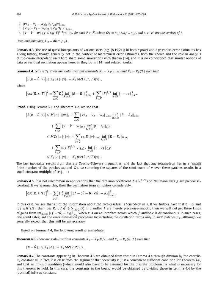
Fig. 6. Initial mesh (colored by solution value) for the jump coefficient problem.

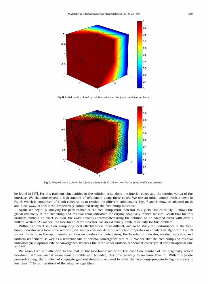
Fig. 7. Adapted mesh (colored by solution value) with 37 458 vertices for the jump coefficient problem.

be found in [17]. For this problem, singularities in the solution arise along the interior edges and the interior vertex of theinterface. We therefore expect a high amount of refinement along these edges. We use an initial course mesh, shown inFig. 6, which is comprised of 8 sub-cubes so as to resolve the different subdomains. Figs. 7 and 8 show an adapted meshand a cut-away of this mesh, respectively, computed using the face-bump indicator.

Again, we begin by studying the performance of the face-bump error indicator as a global indicator. Fig. 9 shows theglobal effectivity of the face-bump and residual error indicators for varying adaptively refined meshes. Recall that for thisproblem, without an exact solution, the exact error is approximated using the solution on an adapted mesh with over 3million vertices. As we see, the face-bump error indicator has an extremely stable effectivity for this problem.

Without an exact solution, computing local effectivities is more difficult, and so to study the performance of the face-bump indicator as a local error indicator, we simply consider its error reduction properties in an adaptive algorithm. Fig. 10shows the error in the approximate solution on meshes computed using the face-bump indicator, residual indicator, and

uniform refinement, as well as a reference line of optimal convergence rate N− 13 . We see that the face-bump and residual

indicators yield optimal rate of convergence, whereas the error under uniform refinement converges at the sub-optimal rateN−0.246.

We again turn our attention to the cost of the face-bump indicator. The condition number of the diagonally scaledface-bump stiffness matrix again remains stable and bounded, this time growing to no more than 11. With this Jacobipreconditioning, the number of conjugate gradient iterations required to solve the face-bump problem to high accuracy isless than 17 for all iterations of the adaptive algorithm.


Fig. 8. Cut-away of adapted mesh (colored by solution value) with 37 458 vertices for the jump coefficient problem.

Fig. 9. Global effectivities of the face-bump and residual error indicators for the jump coefficient problem.

7.3. Convection–diffusion problem

Here we consider a problem with convection in order to test the indicator on a problem which gives a non-symmetricsystem matrix. Specifically, we solve

−ε�u + ux = 1

on the domain Ω = (0,1)3 subject to u(x = 0) = u(x = 1) = 0 and homogeneous Neumann condition on the other four faces.This problem has exact solution independent of y and z given by

u(x, y, z) = x − ex−1ε − e− 1

ε

1 − e− 1ε

.

For these experiments, we used ε = 0.1. The initial course mesh is shown in Fig. 11 while Fig. 12 shows an adapted solutioncomputed using the face-bump indicator.


Fig. 10. Energy norm of the error of a solution computed on a mesh computed using face-bump and residual error indicators, as well as using uniformrefinement for the jump coefficient problem.

Fig. 11. Initial mesh (colored by solution value) for the convection–diffusion problem.

The global and local effectivities are shown in Figs. 13 and 14, respectively. As we see, the face-bump indicator isremarkably robust both locally and globally even in the presence of the convection term. Also shown on Fig. 13 (at theemphasized points) is when the adaptive scheme lowers the mesh Péclet number, given by hmin

ε , to a value below 1, atwhich point the problem behaves like the Poisson equation. Note that with uniform refinement, this doesn’t occur untilthere are around 3000 vertices in the mesh. Fig. 15 shows the convergence profile (in the H1 norm) of the face-bumpand residual indicator-based methods as well as uniform mesh refinement. For this problem, we see that even uniformmesh refinement is able to attain optimal convergence rate, but the adapted meshes still maintain better placement of theunknowns.

Finally, the conditioning of the face-bump stiffness matrix remains well behaved for this problem, remaining at less than9 after diagonal scaling. The number of BiCG iterations with diagonal preconditioning remains bounded by 17 for all stepsof the adaptive process.


Fig. 12. Adapted mesh (colored by solution value) with 10 588 vertices for the convection–diffusion problem.

Fig. 13. Global effectivities of the face-bump and residual error indicators for the convection–diffusion problem.

7.4. Anisotropic diffusion problem

Finally, we consider a problem with an anisotropic diffusion coefficient. Specifically, let the matrix A be the 3×3 diagonalmatrix with diagonal entries 1, ε, ε−1, where ε = 10−3. Then we consider the problem of solving

−∇ · (A∇u) = 1

on the domain Ω = (−1,1)3 subject to homogeneous Dirichlet boundary conditions. This high anisotropy can cause theresidual error indicator to have poor global effectivity [11], and we use this example only to study the effectivity of theface-bump indicator.

The global effectivities of the two indicators are shown in Fig. 16. We note here that, even on the finest meshes, theimportant quantity hmin

ε2 is still greater than 103. The energy norm of the error for both adaptive algorithms as well asuniform refinement are shown in Fig. 17. It is apparent that the face-bump indicator retains its usual stable global ef-fectivity. However the adaptive algorithms are unable to attain optimal convergence rates—likely due to the longest-edgebisection, which does not allow for anisotropic elements. In this case, the matrix for computing ε is ill-conditioned (even


Fig. 14. Maximum, minimum, and average local effectivities of the face-bump and residual error indicators for the convection–diffusion problem.

Fig. 15. H1 norm of the error of a solution computed on a mesh computed using face-bump and residual error indicators, as well as using uniformrefinement for the convection–diffusion problem.

after rescaling) due to the anisotropy in A, which results in more conjugate gradient iterations for the computation of ε.A refinement scheme which allowed for elements which were shape regular with respect to the anisotropic metric inducedby A would likely improve not only the conditioning, but also the convergence of the method; but our primary interesthere was merely to demonstrate that our hierarchical estimator does not suffer the same deficiencies as residual estimatorsin terms of effectivity.


Fig. 16. Global effectivities of the face-bump and residual error indicators for the anisotropic diffusion problem.

Fig. 17. Energy norm of the error of a solution computed on a mesh computed using face-bump and residual error indicators, as well as using uniformrefinement for the anisotropic diffusion problem.

8. Final remarks

We have demonstrated, both theoretically and empirically, the usefulness of a particular hierarchical error estimator, bothin terms of estimating global and local errors, and in driving an adaptive algorithm. The approach implemented here is apractical realization of the general framework given for constructing and analyzing such hierarchical error estimators—onewhich we believe does a very good job of clarifying the relevant issues related to the choice of auxiliary space W in whichthe error is to be estimated, and gives a very clear picture of which aspects of the data the constants and oscillation term


in the reliability bound do (and do not!) depend. It is very natural at this stage to wonder whether or not one can proveconvergence of an adaptive method within this framework, and if non-linear problems can also be adequately addressed.We intend to address these issues in a sequel to the present work.

References

[1] M. Ainsworth, J.T. Oden, A Posteriori Error Estimation in Finite Element Analysis, Pure Appl. Math. (N.Y.), Wiley–Interscience [John Wiley & Sons], NewYork, 2000.

[2] C.B. Allendoerfer, Generalizations of theorems about triangles, Math. Mag. 38 (1965) 253–259.[3] R. Araya, A.H. Poza, E.P. Stephan, A hierarchical a posteriori error estimate for an advection–diffusion–reaction problem, Math. Models Methods Appl.

Sci. 15 (2005) 1119–1139.[4] I. Babuska, W.C. Rheinboldt, Error estimates for adaptive finite element computations, SIAM J. Numer. Anal. 15 (1978) 736–754.[5] R.E. Bank, Hierarchical bases and the finite element method, Acta Numer. 5 (1996) 1–43.[6] M. Bebendorf, A note on the Poincaré inequality for convex domains, Z. Anal. Anwend. 22 (2003) 751–756.[7] F.A. Bornemann, B. Erdmann, R. Kornhuber, A posteriori error estimates for elliptic problems in two and three space dimensions, SIAM J. Numer.

Anal. 33 (1996) 1188–1204.[8] P. Clément, Approximation by finite element functions using local regularization, Rev. Française Automat. Informat. Recherche Opérationnelle Sér.,

RAIRO Analyse Numérique 9 (1975) 77–84.[9] W. Dörfler, A convergent adaptive algorithm for Poisson’s equation, SIAM J. Numer. Anal. 33 (1996) 1106–1124.

[10] W. Dörfler, R.H. Nochetto, Small data oscillation implies the saturation assumption, Numer. Math. 91 (2002) 1–12.[11] F. Fierro, A. Veeser, A posteriori error estimators, gradient recovery by averaging, and superconvergence, Numer. Math. 103 (2006) 267–298.[12] M. Holst, Adaptive numerical treatment of elliptic systems on manifolds, Adv. Comput. Math. 15 (2001) 139–191.[13] P. Morin, R.H. Nochetto, K.G. Siebert, Convergence of adaptive finite element methods, SIAM Rev. 44 (2002) 631–658 (electronic) (2003). Revised reprint

of “Data oscillation and convergence of adaptive FEM”: SIAM J. Numer. Anal. 38 (2) (2000) 466–488 (electronic); MR1770058 (2001g:65157)].[14] P. Morin, R.H. Nochetto, K.G. Siebert, Local problems on stars: a posteriori error estimators, convergence, and performance, Math. Comp. 72 (2003)

1067–1097 (electronic).[15] J.S. Ovall, Duality-based adaptive refinement for elliptic PDEs, PhD thesis, University of California, San Diego, La Jolla, CA 92093, USA, 2004.[16] L.E. Payne, H.F. Weinberger, An optimal Poincaré inequality for convex domains, Arch. Ration. Mech. Anal. 5 (1960) 286–292.[17] M. Petzoldt, A posteriori error estimators for elliptic equations with discontinuous coefficients, Adv. Comput. Math. 16 (2002) 47–75.[18] M.C. Rivara, Local modification of meshes for adaptive and/or multigrid finite-element methods, J. Comput. Appl. Math. 36 (1991) 79–89.[19] L.R. Scott, S. Zhang, Finite element interpolation of nonsmooth functions satisfying boundary conditions, Math. Comp. 54 (1990) 483–493.[20] G. Strang, G.J. Fix, An Analysis of the Finite Element Method, Prentice Hall Ser. Autom. Comput., Prentice Hall Inc., Englewood Cliffs, NJ, 1973.[21] R. Verfürth, Error estimates for some quasi-interpolation operators, M2AN Math. Model. Numer. Anal. 33 (1999) 695–713.

Documents

An efficient, reliable and robust error estimator for elliptic problems in