620 J. GUIDANCE VOL. 8, NO. 5

An Eigensystem Realization Algorithmfor Modal Parameter Identification and Model Reduction

Jer-Nan Juang* and Richard S. Pappa*NASA Langley Research Center, Hampton, Virginia

A method called the eigensystem realization algorithm is developed for modal parameter identification andmodel reduction of dynamic systems from test data. A new approach is introduced in conjunction with thesingular-value decomposition technique to derive the basic formulation of minimum order realization which isan extended version of the Ho-Kalman algorithm. The basic formulation is then transformed into modal spacefor modal parameter identification. Two accuracy indicators are developed to quantitatively identify the systemand noise modes. For illustration of the algorithm, an example is shown using experimental data from theGalileo spacecraft.

Introduction

THE state space model has received considerable attentionfor system analyses and design in recent control and

systems research programs. One of these areas, in particular, iscontrol of large space structures. In order to design controls fora dynamic system it is necessary to have a mathematical modelthat will adequately describe the system's motion. The processof constructing a state space representation from experimentaldata is called system realization.

During the past two decades, numerous algorithms for theconstruction of state space representations of linear systemshave appeared in the controls literature. Among the first werethe works of Gilbert1 and Kalman,2 introducing the importantprinciples of realization theory in terms of the concepts ofcontrollability and observability. Both techniques use thetransfer function matrix to solve the realization problem. Hoand Kalman3 approached this problem from a new viewpoint.They showed that the minimum realization problem isequivalent to a representation problem involving a sequence ofreal matrices known as Markov parameters (pulse responsefunctions). By minimum realization is meant a model with thesmallest state space dimension among systems realized thathas the same input-output relations within a specified degreeof accuracy. Questions regarding the minimum realizationfrom various types of input-output data and the generation ofa minimum partial realization are studied by Tether,4 Silver-man,5 and Rossen and Lapidus6 using Markov parameters.Rossen and Lapidus7 successfully applied Ho-Kalman3 andTether4 methods to chemical engineering systems. A commonweakness of the preceding schemes is that effects of noise onthe data analysis were not evaluated. Zeiger and McEwen8

proposed a combination of the Ho-Kalman algorithm3 withthe singular-value decomposition technique for the treatmentof noisy data. However, no theoretical or numerical studieswere reported by Zeiger and McEwen. Among follow-updevelopments along similar lines, Kung9 presented anotheralgorithm in conjunction with the singular-value decomposi-tion technique to incorporate the presence of the noise. Notethat the singular-value decomposition technique10'11 has beenwidely recognized as being very effective and numericallystable. Although several techniques of minimum realizationare available in the literature, formal direct application to

Received July 3,1984; revision received Nov. 29,1984. This paper isdeclared a work of the U.S. Government and therefore is in the publicdomain.

*Aerospace Engineer, Structural Dynamics Branch. MemberAIAA.

modal parameter identification for flexible structures has notbeen addressed.. . .

In the structures field, the finite element technique is usedalmost exclusively for constructing analytical models. This ap-proach is well established and normally provides a model ac-curate enough for structural design purposes. Once the struc-ture is built, static and dynamic tests are performed. These testresults are used to refine the finite element model, which isthen used for final analyses. This traditional approach toanalytical model development may not be accurate enough foruse in designing a vibration control system for flexible struc-tures. Another approach is to realize a model directly from theexperimental results. This requires the construction of aminimum-order model from the test data that characterizesthe dynamics of the system at the selected control andmeasurement positions. The present state-of-the-art in struc-tural modal testing and data analysis is one of controversyabout the best technique to use. Classical test techniques,which may provide only good frequency and moderate modeshape accuracy, are often considered adequate for finite ele-ment model verification purposes. On the other hand, ad-vanced data analysis techniques that offer significant reduc-tions in test time and improved accuracy have beenavailable,12'16 but are not yet fully accepted. For example,Void and Russell16 presented a method using frequency-response functions and time-domain analysis for direct iden-tification of modal parameters including repeated eigenvalues.A comparison of contemporary methods using data from theGalileo spacecraft test is provided by Chen.17

Although structural dynamics techniques are generally suc-cessful for ground data, further incorporation with work fromthe controls discipline is needed to solve modal parameteridentification/control problems. For example, it is knownfrom control theory18 that a system with repeated eigenvaluesand independent mode shapes is not identifiable by single in-put and single output. Methods which allow only one initialcondition (input) at a time13 will miss repeated eigenvalues.Also, if the realized system is not of minimum order andmatrix inversion is used for constructing an oversized statematrix, numerical errors may become dominant.

Under the interaction of structure and control disciplines,the objective of this paper is to introduce an eigensystemrealization algorithm (ERA) for modal parameter identifica-tion and model reduction for dynamical systems from testdata. The algorithm consists of two major parts, namely,basic formulation of the minimum-order realization andmodal parameter identification. In the section of the basic for-mulation, the Hankel matrix, which represents the data struc-ture for the Ho-Kalman algorithm, is generalized to allow ran-

SEPT.-OCT. 1985 MODAL PARAMETER IDENTIFICATION AND MODEL REDUCTION 621

dom distribution of Markov parameters generated by freedecay responses. A unique approach based on this generalizedHankel matrix is developed to extend the Ho-Kalmanalgorithm in combination with the singular-value decomposi-tion technique.10'11 Through the use of the generalized Hankelmatrix, a linear model is realized for a dynamical systemmatching the input and output relationship. The realizedsystem model is then transformed into modal space for modalparameter identification. As part of ERA, two accuracy in-dicators, namely, the modal amplitude coherence and themodal phase collinearity, are developed to quantify the systemand noise modes. The degree of modal excitation and observa-tion is evaluated. The ERA method thus forms the basis for arational choice of model size determined by the singular valuesand accuracy indicators.

Experimental results for a complex structure—the Galileospacecraft—are given to illustrate the ERA method. TheGalileo spacecraft is an interplanetary vehicle to be launchedin 1986 for a detailed investigation of the planet Jupiter and itsmoons.

Basic FormulationsA finite dimensional, discrete-time, linear, time-invariant

dynamical system has the state-variable equations

x(k+l)=Ax(k)+Bu(k)

y(k)=Cx(k)

(1)

(2)

where x is an ^-dimensional state vector, u an m-dimensionalcontrol input, and y a p-dimensional output or measurementvector. The integer k is the sample indicator. The transitionmatrix A characterizes the dynamics of the system. For flexi-ble structures, it is a representation of mass, stiffness, anddamping properties. The problem of system realization is asfollows: Given the measurement functions y(k), constructconstant matrices [A, B, C] such that the functions y arereproduced by the state-variable equations. Any system has aninfinite number of realizations that will predict the identicalresponse for any particular input. Let T be any nonsingularsquare matrix. The triple [TAT'1, TB, CT'1] will also be arealization.6 However, the eigenvalues of the matrix A arepreserved.

For the system Eqs. (1) and (2) with free pulse response, thetime domain description is given by the function known as theMarkov parameter

Y(k)=CAk-*B (3)

or in the case of initial state response

Y(k)=CAk[x1(0),x2(0),...,xm(0)]

where x/(0) represents the rth set of initial conditions and k isan integer. Note that B is an n x m matrix and C is a p x nmatrix. The problem of system realization is: Given the func-tions Y(k), construct constant matrices [A,B,C] in terms ofY(k) such that the identities of Eq. (3) hold. The algorithmbegins by forming the r x s block matrix (generalized Hankelmatrix)

Y(k)

... Y(j1 + k+ts_1)

_ Y(Jr-i+V YUr-i

where y / ( /= !,...,/*—1) and */(/= l,...,s — 1) are arbitrary in-tegers. For the system with initial state responsemeasurements, simply replace Hrs(k-\) by Hrs(k). Nowobserve that

C

CA>*

CAjr-l

and

Ws=[B,A'iB,...,A's-iB] (5)

where Vr and Ws are the observability and controllabilitymatrices, respectively. Note that Vr and Ws are rectangularmatrices with dimensions rp x n and n x ms, respectively.Assume that there exists a matrix If satisfying the relation

(6)

where In is an identity matrix of order n. It will be shown thatthe matrix IP plays a major role in deriving the ERA. What is//*? Observe that, from Eqs. (5) and (6),

(7)

The matrix If is thus the pseudoinverse of the matrix Hrs(0) ina general sense. For a single input, there exists a case [see Eq.(5)] where the rank of Hrs(0) equals the column number ofHn(0), then

H«=[[Hrs(0)]THrs(0)]-J[Hrs(0)]T (8)

On the other hand, there exists a case for a single output [seeEq. (5)] where the rank equals the row number, then

H#=[Hrs(0)]T(Hrs(0)[Hrs(0)]T]-1 (9)

The matrix Hrs(l)H* has been used in the structural dynamicsfield to identify system modes and frequencies.13 This is aspecial case representing a single input which cannot realize asystem that has repeated eigenvalues, or a noise-free systemunless the system order is known a priori. More discussion canbe found in the Appendix.

A general solution for If is given below. For an «th-ordersystem, find the nonsingular matrices P and Q such that 1(U1

Hrs(0)=PDQT (10)

where the rpxn matrix P and the msxn matrix Q areisometric matrices (all of the columns are orthonormal), leav-ing the singular values of Hrs(Q) in the diagonal matrix D withpositive elements [d1,d2,...,dn]. The rank n of Hrs(G) is deter-mined by testing the singular values for zero (relative todesired accuracy)11 which will be described in the next section.Define

Hn(0) =PDQT= [PD] [QT] = (11)

Each of the four matrices [Pd,QT, Ws, V?] has rank and rownumber n. By Eq. (5) with fc = 0, ,

VrWs=Hrs(0)=PdQT (12)

Multiplying on the left by Pj and solving for QT yields

(4) TWs=(PTdPd)~1PT

dVrWs = (13)

622 J.-N. JUANG AND R.S. PAPPA J. GUIDANCE

The matrix T is nonsingular because if

then TU=Iby Eq. (13). Since 7T/=/= LTfor nonsingular Tand C/, then

Hence, by Eq. (14),

= [Q]

(14)

(15)

The dimension of matrices Q and Pj with rank n are msxnand « x 77?, respectively. Define 0^ as a null matrix of order/?,Ip an identity matrix, Ej= [/^O^...^], and £%=[!„,Ow,...,0m].

With the aid of Eqs. (5), (6), and (15), a minimum order-realization can be obtained from

Y(k+l)=ETpHrs(k)Em=ET

pVrAkWsEm

= ETpVrWsH*VrAkWsH»VrWsEm

=ElHrs(0)QP»dVrAkWsQP»dHrs(0)Em

(16)

=EtPd[P»dHK(l)Q]*QTEm

=ETpD'A[D-'APTHK(l)QD-'A]kDKQTEfft

This is the basic formulation of realization for the ERA. Thetriple [D-1/2PTHrs(\)QD~1/2, D1/2QTEmJ ET

pPD1/2 ] is aminimum realization since the order n of P*dHrs(\)Q equals thedimension of the state vector x. The same solution, in a dif-ferent form, for the case wherey, = */ = / (/= l,...,r-1), can beobtained by a completely different approach as shown in Refs.3 and 19. The system [Eqs. (1) and (2)] with this realization iswritten as

x(k+l)=D-'/2PTHrs(l)QD-1/2x(k)+D'/2QTEmu (17)

wherey(k)=ETPD1/2x(k)

= WsQD~1/2x(k)

(18)

(19)

Now, the case can be summarized as follows.A finite dimensional, discrete-time, linear time-invariant

dynamical system with multi-input and multi-output isrealizable in terms of the measurement functions if the systemis controllable and observable (the ranks of matrices Vr andWs are n). A simple exercise, such as replacing Y(k+\) byY(k) in Eq. (16), shows that the algorithm developed above isalso true for the realization of a system with initial stateresponse.

Note that no restrictions on system eigenvalues are given forthis case. In other words, this technique can realize a systemwith repeated eigenvalues. As byproducts of this approach,two alternative algorithms identified as (Al) and (A2) arederived in the Appendix.

Modal Parameter Identificationand Model Reduction

The presence of almost unavoidable noise and structuralnonlinearity introduces uncertainty about the rank of thegeneralized Hankel matrix and, hence, about the dimension ofthe resulting realization. By employing the singular-valuedecomposition (SVD) technique, the rank structure of the

Hankel matrix can be displayed quantitatively. The set ofsingular values can be used to judge the distance of the matrixwith determined order to a lower-order one. Therefore, thestructure of the generalized Hankel matrix can be properly ex-ploited to solve the realization problem efficiently. These in-clude an excellent numerical performance, stability of therealization, and flexibility in determining order-error tradeoff.

Assume that, by Eq. (10),

with

(20)

(21)

If the matrix Hrs(0) has rank n then all of the singular valuesdf (i = n + 1,..; ,N) should be zero. When singular valuesdt (i = n +1,...,N) are not exactly zero but very small, then onecan easily recognize that the matrix Hrs(G) is not far awayfrom an w-rank matrix/However, there can be real difficultiesin determining a gap between the computed last nonzerosingular value and what effectively should be considered zero,when measurement noise is present. Possible sources of thenoise can be attributed to the measurement signal, computerroundoff, and instrument imperfections.

Look at the singular value dn of the matrix Hrs(G). Choose anumber d based on measurement errors incurred in estimatingthe elements of Hrs(Q) and/or roundoff errors incurred in aprevious computation to obtain them. If d is chosen as a "zerothreshold" such that d<dn, then the matrix Hrs(Q) is con-sidered to have rank n. Unless information about the certaintyof the measurement data is given, the number d is defined as afunction of the precision limit in the computer. For example,b-dn/dj cannot exceed the precision limit; further details arefound in Ref. 11.

After the test of singular values, assume that the matrix[D-1/2PTHrs(k)QD~1/2} has rank n. Find the eigenvalues zand eigenvectors ^ such that

(22)

The modal damping rates and damped natural frequencies aresimply the real and imaginary parts of the eigenvalues, aftertransformation from the z to the s plane using the relationship

(23)

where AT is the data sampling interval andy is an integer. Theinteger k is generally chosen as 1 for simplicity. Although zand \// are complex numbers, computations of Eq. (22) can beperformed using a real algorithm20 since the state matrixrealized for flexible structures has independent eigenvectors.

The triple [z, ^-lD1/2QTEm) ETpPD1/2^\ is obviously a

minimum order realization simply by observing Eq. (16). Thematrix E*PD1/2\I/ is called mode shapes and the matrix^-1D1/2Q^Em initial modal amplitudes. To quantify thesystem and noise modes, two indicators are developed asfollows.

Modal Amplitude Coherence yIf the information about the uncertainties of the measure-

ment is minimum, the rank thus determined by the SVDbecomes larger than the number of excited and observedsystem modes to represent the presence of noises in modalspace. In modal parameter identification, the indicator refer-red to as modal amplitude coherence is developed to quan-titatively distinguish the system and noise modes. Based on theaccuracy parameter, the degree of modal excitation (con-trollability) is estimated.

The modal amplitude coherence is defined as the coherencebetween each modal amplitude history and an ideal one

SEPT.-OCT. 1985 MODAL PARAMETER IDENTIFICATION AND MODEL REDUCTION 623

formed by extrapolating the initial value of the history to lat-ter points using the identified eigenvalue. Let the control inputmatrix (initial condition) be expressed as

is then defined as21

(24)

where the asterisk means transpose complex conjugate, andthe Ixm column vector 2?y corresponds to the system eigen-value $j (j = !,...,«)• Consider the sequence

(25)

which represents the ideal modal amplitude in the complex do-main containing information of the magnitude and phaseangle with time step AT. Now, define vector q^ such that

\I/~1D1/2QT= [qlfq23...fqn]* (26)

The comrjlex vector </, represents the modal amplitude timehistory from the real measurement data obtained by thedecomposition of the Hankel matrix. Let 7, be defined as thecoherence parameter for the y'th mode, satisfying the relation

7;= (27)

where I I represent the absolute value. The parameter 7, canhave only the values between 0 and 1. 7,-* 1 as q} ̂ qj indicatesthat the realized system eigenvalue Sj and the initial modalamplitude bj are very close to the true values for the y'th modeof the system. On the other hand, if 7, is far away from thevalue 1, the y'th mode is a noise mode. However, to make aclear distinction between the system and noise modes requiresfurther study. Obviously, the parameter 7, quantifies thedegree to which the modes were excited by a specific input,i.e., the degree of controllability.

Modal Phase Collinearity /*For lightly damped structures, normal mode behavior

should be observed., An indicator referred to as the modalphase cbllinearity is developed to measure the strength of thelinear functional relationship between the real and imaginaryparts of the mode shape for each mode. Based on the accuracyindicator, the degree of modal observation is estimated.Define

ETpPD1/^=[c1,c2,...,cn] (28)

where Cj (j = 1,2,...,«) is the mode shape corresponding to they'th realized mode. Let the column vector 7 of order p be

7T=[7,7,...,7] (29)

in which p is the number of sensors. Now compute the follow-ing quantities for the y'th mode shape.

(30)

(31)

(32)

(33)

(34)

(35)

where Re( ) and Im( ), respectively, are the real and imag-inary parts of the complex vector ( ), and sgn( ) is the sign ofthe scalar ( ). The modal phase collinearity /*, for the y'th mode

cri=[Re(Cj-Cjl)]T[Im(Cj-Cjl)]

e=(cn-crr)/2cri

j = l,2,...,n (36); • } • ..;-

This indicator checks the deviation from 0-180 degreebehavior for components of the y'th identified mode shape.The parameter ^j can have only the values between 0 and 1.fjij — 1 indicates that accuracy of the mode shape is high. Onthe other hand, if /*, is away from 1, the y'th mode is either anoise mode or the mode is significantly complex.

Model ReductionThe dynamical system is composed of an interconnection of

all of the ERA-identified modes. The accuracy indicatorsallow one to determine the degree of individual mode par-ticipation. Model reduction then can be made by truncating allof the modes with low accuracy indicators. The accuracy ofthe complete modal decomposition process can be examinedby comparing a reconstruction of Y(k) formed by Eq. (16)with the original free decay responses, using the reducedmodel.

Summary of ERAThe computational steps are summarized as follows:1) Construct a block-Hankel matrix 7/r5(0) by arranging the

measurement data into the blocks with givdn r, s, tt (i =1,2,...,5-7) andy /(i=l,2,...,r-l), [Eq. (4)].

2) Decompose Hrs(G) using singular-value decomposition[Eq. (10)].

3) Determine the order of the system by examining thesingular values of the Hankel matrix Hrs(Q) [Eq. (20)].

4) Construct a minimum-order realization (A, B, C) usinga shifted block-Hankel matrix [Eq. (16)].

5) Find the eigensolution of the realized state matrix [Eq.(22)] and compute the modal damping rates and frequencies[Eq.(23)].

6) Calculate the coherence parameter [Eq. (27)] and thecollinearity parameter [Eq. (36)] to quantify the system andnoise modes.

7) Determine the reduced system model based on the ac-curacy indicators, reconstruct function Y(k) [Eq. (16)], andcompare with the measurement data.

Note that the optimum determination of r, s, t; andy, in step1 above requires further development. This determination isrelated to the choice of the measurement data to minimize thesize of the Hankel matrix Hrs (0) with the rank unchanged.

RPM THRU STIRCLUSTERSBA400 N. ENGINE

SCANPLATFORM

S/C ADAPTERSSEISMICBLOC

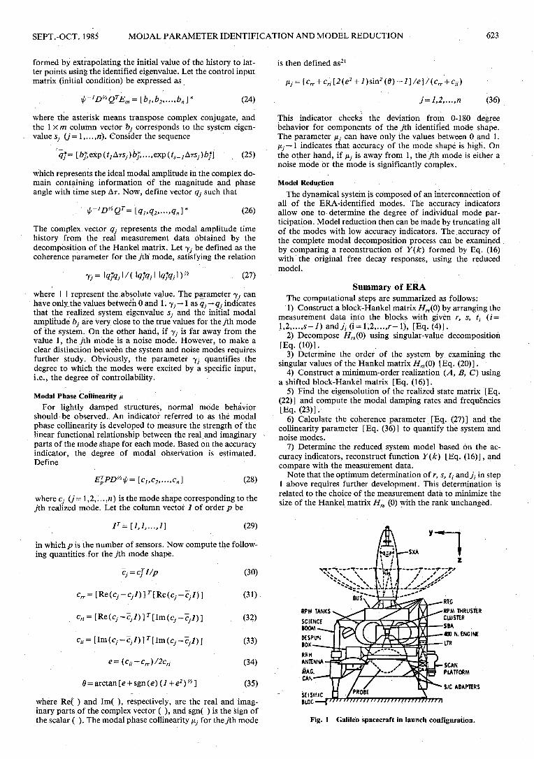
Fig. 1 Galileo spacecraft in launch configuration.

624 J.-N. JUANG AND R.S. PAPPA J. GUIDANCE

Example: Analysis of Galileo Test Datathe ERA method has been verified using multi-input and

multi-output simulation data with or without noise for as-sumed structures with distinct and/or repeated eigenvalues.The reader is directed to the original version of this paper22 formore information. Experimental results for the analysis ofGalileo test data are given in the following.

The Galileo spacecraft is shown in Fig. 1. All appendages,including the S-X-band antenna (SXA) at the top of the vehi-cle, were locked in their stowed positions. The structure wascantilevered from its base by bolting the bottom edge of theconical spacecraft adapter ring to a massive seismic block. Theadapter ring is the interface between Galileo and a Centaur up-per stage that will provide the interplanetary boost.

For dynamic excitation, several electrodynamic shakers ofabout 100 N capacity, hung on soft suspensions fromoverhead cranes, were attached at various points. Responsemeasurements were made with 162 accelerometers distributedover the test article.

The finite element model of the structure in this configura-tion predicted 45 modes of vibration below 50 Hz, with thelowest frequency at about 13 Hz. However, as discussed inRef. 23, many of the modes are of lesser importance based ontheir predicted contribution to the dynamic launch loads. Infact, only about 15 modes are major contributors. Thepresence of the others, however, interspersed., in frequencywith the important ones, results in high modal density andmakes accurate parameter identification more difficult.

Complete details of the test configuration, analytical modelpredictions, and the method used to estimate the relative im-portance of the modes, can be found in Ref. 23.

Test and Data Acquisition ProceduresAll results to be presented were obtained from two sets of

free-response measurements recorded following single-pointrandom excitation of the structure. The first data set was ob-tained using single-shaker, lateral excitation—in the global Xdirection—and the second set with single shaker, vertical ex-citation—in the global z direction. These tests are referred toas simply the "x direction" and "z direction" tests. For bothtests, no special effort was made to select the position for theshaker. Each position was chosen using only the knowledgethat many modes were excited from the location in previoustests. Other than the point and direction of excitation, all

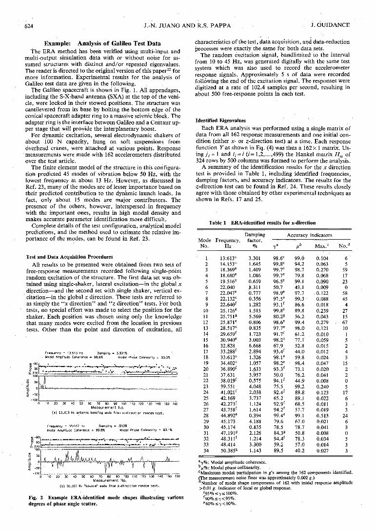
Frequency = 13.613 Hz Damping = 3.301%Modal Amplitude Coherence = 98.6% Modal Phase Colinearity = 99.0%

<u-90Mo 900.270

100

| 50

f °

| -50-100

«»....*....».......,.. ... •*..».,.».'•.., — 2u*M — ,.~.> .• >.•*,*• .t ^

JL0 10 20 30 40 50 60 70 80 90 100 110 120 130 140 150 160

Measurement No.(a) 13.613 Hz antenna bending mode from x-direction random test.

Frequency = 38.037 Hz Damping = .513%Modal Amplitude Coherence = 99.8% Modal Phase Colinearity = 93.1%

0 10 20 30 40 50 60 70 80 .90 100 110 120 130 140 150 160Measurement No.

(b) 38.037 Hz "bounce" mode from z-direction random test.

Fig. 2 Example ERA-identified mode shapes illustrating variousdegrees of phase angle scatter.

characteristics of the test, data acquisition, and data-reductionprocesses were exactly the same for both data $ets.

The random excitation signal, bandlimited to the intervalfrom 10 to 45 Hz, was generated digitally with the same testsystem which was also used to record the accelerometerresponse signals. Approximately 5 s of data were recordedfollowing the end of the excitation signal. The responses weredigitized at a rate of 102.4 samples per second, resulting inabout 500 free-response points in each test.

Identified EigenvaluesEach ERA analysis was performed using a.single matrix of

data from all 162 response measurements and one initial con-dition (either x- or z-direction test) at a time. Each responsefunction Yas shown in Eq. (4) was thus a 162x 1 matrix. Us-ing jj = 1 and tf = i (i= 1,2,...,499) the Hankel matrix Hrs of324 rows by 500 columns was formed to perform the analysis.

A summary of the identification results for the x directiontest is provided in Table 1, including identified frequencies,damping factors, and accuracy indicators. The results for thez-direction test can be found in Ref. 24. These results closelyagree with those obtained by other experimental techniques asshown in Refs. 17 and 25.

Table 1 ERA-identified results for x-direction

ModeNo.

123456789

10111213141516171819202122232425262728293031323334

Frequency,Hz

13.613s

14.153s

18.369s

18.680s

19.516s

22.04022.0476

22.132s

22.640f

25.126s

25.751g

25.871s

28.517s

29.659f

30.940s

32.82833.288f

33.613s

34.402s

36.890f

37.63138.019f

39.55141.021f

42.16942.273f

43.758f

44.892s

45:17345.17447.191g

48.311f

48.41450.3858

Darnpingfactor,

3.3011.6451.4091.0860.6593-3110.7770.3561.2821.5155.5690.8060.8351.7233.0036.6682.8941.3261.0571.6335.9570.5754.0482.0383.7371.1241.6140.3944.1880.8352.1261.2143.3001.143

Accuracy

Ta

98.6s

99.8s

99.7s

99.7s

96.5s

50.798.9s

97.5s

93. lf

99.8s

80.2g

98.6s

97.7s

91.7f

98.2s

67.993. 4f

98.1s

98.2s

93.3f

50.094. lf

75.592.4f

65.292.9f

94.2f

99.4s

79.678.584.3g

94.4f

59.289.5

M*

99.094.298.779.899.143.197.799.386.689.856.299.498.061.277.152.844.059.898.473.176.244.999.289.889.168.557.799.167.078.750.878.357.040.2

indicators

Max.c

0.1040.0630.2700.0680.0900.0090.1220.0880.0180.2390.0430.2790.1210.0100.0590.0150.0120.0240.0470.0200.0410.0080.2400.1230.0220.0110.0190.5130.0210.0410.0080.0340.0140.027

No.d

65

5917230

58454

2715671015243

152205

17633

24630533

a7%: Modal amplitude coherence.bfjL%: Modal phase collinearity.cMaximum modal participation in g's among the 162 components identified.(The measurement noise floor was approximately 0.002 g.)"Number of mode shape components of 162 with initial response amplitude>0.01 g. Indicator of local or global response.

f90<7o<7<95«7o.

SEPT.-OCT. 1985 MODAL PARAMETER IDENTIFICATION AND MODEL REDUCTION 625

The best single accuracy indicator now available is themodal amplitude coherence. Its value is used in Table 1 to ratethe identified modes at various degrees of accuracy. The ratingscale is noted in the key beneath the table. A brief descrip-tion of the information in each of the three columns on the farright of the table is also contained in the keys. The significanceof modal phase collinearity will be discussed in the nextsubsection. The data in the last two columns are two addi-tional indications of the strength of the modal response signalsrelative to the instrumentation noise floor. These indicatorsare computed using modal participation values in physicalunits, which are the products of the mode shapes and the in-itial modal amplitudes.

Identified Mode ShapesTwo typical ERA-identified mode shapes are shown in Fig.

2. Based on these results and observations from other data notshown, the following conclusions can be drawn.

1) The local behavior of many of the Galileo modes—ex-emplified by the antenna mode shown in Fig. 2a in which onlyabout five measurements show motion—makes it more dif-ficult to identify all 162 components of the mode shapes ac-curately because of the low response levels. • *;*

2) A good measure of the effects of noise on the modeshape accuracy is often indicated by the amount of scatter inthe identified modal phase angles from the ideal 0-180 degnormal mode behavior. Of course, true complex-modebehavior needs to be differentiated from identification scatterdue to noise and nonlinearity. The best remedy is to comparethe results for the same mode obtained in several differenttests.

3) The parameter referred to as the modal phase collinear-ity can be used to measure how closely the modal phase angleresults for each mode cluster near 0 and 180 deg. Calculatedusing principal component analysis, it indicates the extent towhich the information in each complex-valued mode shape isrepresentable as a real-valued vector. It ranges from a value ofzero for no collinearity to 100% for perfect collinearity.

4) Based on studies with simulated data, the accuracy ofmode shapes showing clustering of the identified phase anglesnear 0 and 180 deg, such as in Fig. 2, can generally be acceptedwith little questioning. However, those modes withsignificantly more phase angle scatter should not be usedwithout further confirmation.

5) Most mode-shape components whose identified phaseangles are displaced from the 0- and 180-deg lines are thosewith the smallest amplitudes. This characteristic is consistentlyobserved in the result shown in Fig. 2b. Small modalamplitude results for these components, however, usually in-dicate accurately that the response amplitude is, in fact, verysmall. This information is all that can be expected from ameasurement standpoint, and is all that is required in manyinstances.

Identified Modal AmplitudesThe ERA modal amplitude coherence indicates the purity of

the individual modal amplitude time histories. For each iden-tified eigenvalue, a modal amplitude time sequence is obtainedfor each initial condition. These data provide a direct indica-tion of the strength with which the mode was identified in theanalysis. For strongly identified modes, the modal amplitudehistory is a pure, exponentially decaying sinusoid of the cor-responding frequency and damping, which decays smoothlyover the entire analysis interval. For weakly identified modes,the modal amplitude history is distorted. In particular, thehistory is a sequence of noise for any eigenvalue not cor-responding to a structural mode.

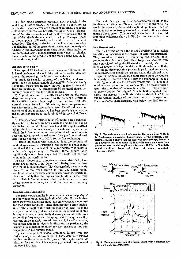
Typical examples of modal amplitude results from theGalileo analysis are shown in Fig. 3. These data were selectedto illustrate the variation in the purity of the modal amplitudehistories for a mode which was strongly excited is only one ofthe two ERA tests.

The mode shown in Fig. 3, at approximately 38 Hz, is thefundamental z-direction "bounce mode" of the structure. Aswould be expected, the modal amplitude plots confirm thatthe mode was more strongly excited in the ^-direction test thanin the x-direction test. This conclusion is reflected in the modalamplitude coherence shown in Fig. 3a compared with that inFig. 3b.

Data ReconstructionThe final aspect of the ERA method available for assessing

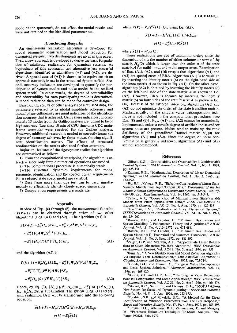
identification accuracy is the process of data reconstruction.This procedure consists of comparing the original free-response, time histories (and their frequency spectra) withthos^e calculated using the ERA-reduced model, which con-tains 22 modes with high modal amplitude coherence. If theERA modal decomposition process is performed accurately,the reconstruction results will closely match the original data.

Figure 4 shows a typical such comparison from the Galileodata analysis. The two time histories are compared at the topof the figure, and their fast Fourier transforms (FFT), in bothamplitude and phase, in the lower plots, the reconstructionresult, the smoother of the two lines in the FFT plots, is seento closely follow the original data in both amplitude andphase. The increase in amplitude of the test data below 2 Hz isdue to residual motion of the shaker on its soft suspension.These response characteristics, well below the first flexural

10°

io-2

2 .3Time, sec

b) 2 3Time, sec

Fig. 3 Example modal amplitude results. This mode near 38 Hz isthe fundamental z-direction "bounce mode" of the structure. Com-parison of a and b shows that the mode was more strongly excited inthe z-directipn test, as ekpected. a) 38.037-Hz modal amplitude from^-direction test; modal amplitude coherence = 99.8%. b) 38.019-Hzmodal amplitude from ^-direction test; modal amplitudecoherence = 94.1%.

AcceL,9

•^ReconstructionLRecc

'JfcAcceL,

.06

0 4 8Time, sec

Measurement

0 4 8Time, sec

180iFFT J rRecOnstr.

Phase °-1801

10'

10

FFT 1Q-4Modulus10

• 2 . . M , , . M M " M | . M . | M M J M M | . U . , , M . | . M . ! , . ? . ,

10 20 30 40 50Frequency, Hz

Fig. 4 Example comparison of a measurement from jc-directioh testwith a 22-mode reconstruction.

626 J.-N. JUANG AND R.S. PAPPA J. GUIDANCE

mode of the spacecraft, do not affect the modal results andwere not retained in the identified parameter set.

Concluding RemarksAn eigensystem realization algorithm is developed for

modal parameter identification and model reduction fordynamical systems. Two developments are given in this paper.First, a new approach is developed to derive the basic formula-tion of minimum realization for dynamical systems. Asbyproducts of this approach, two alternative less powerfulalgorithms, identified as algorithms (Al) and (A2), are de-rived. A special case of (A 1) is shown to be equivalent to anapproach currently in use in the structural dynamics field * Sec-ond, accuracy indicators are developed to quantify the par-ticipation of system modes and noise modes in the realizedsystem model. In other words, the degree of controllabilityand observability for each participating mode is determined.A model reduction then can be made for controller design.

Based .on the results of other analyses of simulated data, theparameters referred to as modal amplitude coherence andmodal phase coliinearity are good indicators of the identifica-tion accuracy that is achieved. Using these indicators, approx-imately 15 modes from the Galileo analysis are judged to be ofhigh accuracy. Less than 10 min of CPU time on a CDC main-frame computer 'were required for the Galileo analysis.However, additional research is needed to correctly assess thedegree of accuracy achieved by those modes showing signifi-cant identification scatter. The effects of structuralnbnlinearities oil the results also need further attention.

Important features of the eigensystem realization algorithmare summarized as follows.

1) From the computational standpoint, the algorithm is at-tractive since only simple numerical operations are needed.

2) The computational procedure is numerically stable.3) The structural dynamics requirements for modal

parameter identification and the control design requirementsfor a reduced state space model are satisfied.

4) Data from more, than one test can be used simulta-neously to efficiently identify closely spaced eigenvalues.

5) Computation requirements are moderate.

AppendixIn view of Eqs. (4) through (6), the measurement function

Y(k+\) can be obtained through either of two otheralgorithms [Eqs. (Al) and (A2)] . The algorithm (Al) is

=E}[Hi,(l)If-]*»H(0)Em

and the algorithm (A2) is

(Al)

=ETpVrWs[H*VrAWs]kEm

(A2)

Hence, by Eq. (3), {Hn(\)If Hrs(Q)Em, ETp} or [H«Hrs(\),

Ey, £jjF/rs(0)] is a realization. The system [Eqs. (1) and (2)]with realization (Al) will be transformed into the followingequation:

x(k+l)=Hrs(l)H»x(k)+Hrs(0)Emu

where x(k) = Vrtfx(k). Or, using Eq. (A2),

x(k+l)=fl»Hrs(l)x(k)+Emu

y(k)=ETpHrs(0)x(k)

where x(k) = Wsx(k).These realizations are not of minimum order, since the

dimension of x is the number of either columns or rows of thematrix Hrs(0) which is larger than the order n of the statematrix A for multi-input and multi-output cases. Examinationof Eqs. (Al), (A2), and (16) reveals that algorithms (Al) and(A2) are special cases of ERA. Algorithm (Al) is formulatedby inserting the identity matrix (6) on the right-hand side ofthe state matrix A as shown in Eq. (Al). On the other hand,algorithm (A2) is obtained by inserting the identity matrix (6)on the left-hand side of the state matrix A as shown in Eq.(A2). However, ERA is formed by inserting the identitymatrix (6) on both sides of the state matrix A as shown in Eq.(16). Because of the different insertion, algorithms (Al) and(A2) do not minimize the order of the state transition matrix.Mathematically, if the singular-value decomposition tech-nique is not included in the computational procedures [seeEqs. (8) and (9)], Eqs. (A 1) and (A2) cannot be numericallyimplemented, unless a certain degree of artificial noise and/orsystem noise are present. Noises tend to make up the rankdeficiency of the generalized Hankel matrix Hrs(0) foralgorithms (Al) and (A2). Since the degree of noise con-tamination is generally unknown, algorithms (Al) and (A2)are not recommended.

<f- .References

Gilbert, E.G., "Controllability and Observability in MultivariableControl Systems," SIAM Journal on Control, Vol. 1, No, 2, 1963,pp. 128-151.

2Kalman, R.E;, "Mathematical Description bf Linear DynamicalSystems," SIAM Journal on Control, Vol. 1, No. 2, 1963, pp.152-192.

3Ho,B.L.,Kalman, R.E., "Effective Construction of Linear State-Variable Models from Input/Output Data," Proceedings of the 3rdAnnual Allerton Conference on Circuit and System Theory, 1965, pp.449-459; also, Regelungstechnik, Vol. 14, 1966, pp. 545-548.

4Tether, A.J., "Construction of Minimal Linear State-VariableModels from Finite Input-Output Data," IEEE Transactions onAutomatic Control, Vol. AC-15, No. 4, Aug. 1970, pp. 427-436.

5Silverman, L.M., "Realization of Linear Dynamical Systems,"IEEE Transactions on Automatic Control, Vol. AC-16, No. 6, 1971,pp. 554-567.

6Rosseh, R.H., and Lapidus, L., "Minimum Realizations andSystem Modeling: I. Fundamental Theory and Algorithms," AIChEJournal, Vol. 18, No. 4, July 1972, pp. 673-684.

7Rossen, R.H.. and Lapidus, L., "Minimum Realizations andSystem Modeling: II. Theoretical and Numerical Extensions," AIChEJournal, Vol. 18, No. 5, Sept. 1972, pp. 881-892.

8Zeiger, H.P. and McEwen, A.J., "Approximate Linear Realiza-tions of Given Dimension Via Ho's Algorithm," IEEE Transactionson Automatic Control, Vol. AC-19, No. 2, April 1974, pp. 153.

9Kung, S., "A New Identification and Model Reduction AlgorithmVia Singular Value Decomposition," 12th Asilomar Conference onCircuits, Systems and Computers, Nov. 1978, pp. 705-714.

10Golubi G.H. and Reinsch, C., "Singular Value Decompositionand Least Squares Solutions," Numerical Mathematics, Vol. 14,1970, pp. 403-420.

uKlema, V.C. and Laub, A.J., "The Singular Value Decomposi-tion: Its Computation and Some Applications," IEEE Transactionson Automatic Control, Vol. AC-25, No. 2, April 1980, pp. 164-176.

12Stroud, R.C., Smith, S., and Hamma, G.A., "MODALAB—ANew System for Structural Dynamic Testing," Shock and VibrationBulletin, No. 46, Pt. 5, Aug. 1976, pp. 153-175.

13Ibrahim, S.R. and Mikulcik, B.C., "A Method for the DirectIdentification of Vibration Parameters from the Free Response,"Shock and Vibration Bulletin, No. 47, Pt. 4, Sept. 1977, pp. 183-198.

14Brown, D.L., Allemang, R.J., Zimmerman, R. and Mergeay,M., "Parameter Estimation Techniques for Modal Analysis," SAEPaper 790221, Feb. 1979.

SEPT.-OCT. 1985 MODAL PARAMETER IDENTIFICATION AND MODEL REDUCTION 627

15Coppolino, R.N., "A Simultaneous Frequency Domain Tech-nique for Estimation of Modal Parameters from Measured Data,"SAE Paper 811046, Oct. 1981.

16Void, H. and Russell, R., "Advanced Analysis Methods ImproveModal Test Results," Sound and Vibration, March 1983, pp. 36-40.

17Chen, J.C., "Evaluation of Modal Testing Methods," AIAAPaper 84-1071, May 1984.

18Chen, C.T., Introduction to Linear System Theory, Holt,Rienhart, and Winston, Inc., New York, 1970.

19Kalman, R.E., and Englar, T.S., "Computation of a MinimalRealization," A User Manual for the Automatic Synthesis Program,NASA CR-475, June 1966, Chap XV.

20Gantmacher, F.R., The Theory of Matrices, Vol. 1, ChelseaPublishing Co., New York, New York, 1959.

21 Moore, B.C., "Principal Component Analysis in Linear Systems:Controllability, Observability, and Model Reduction," IEEE Trans-actions on Automatic Control, Vol. AC-26, No. 1, Feb. 1981, pp.17-32.

22Juang, J.N. and Pappa, R.S., "An Eigensystem RealizationAlgorithm (ERA) for Modal Parameter Identification and ModelReduction," NASA/JPL Workshop on Identification and Control ofFlexible Space Structures, San Diego, Calif., June 1984.

23Chen, J.C. and Trubert, M., "Galileo Modal Test and Pre-TestAnalysis," Proceedings of the 2nd International Modal Analysis Con-ference, Orlando, Fla., Feb. 1984, pp. 796-802.

24Pappa, R.S. and Juang, J.N., "Galileo Spacecraft Modal Iden-tification Using an Eigensystem Realization Algorithm," The Journalof the Astronautical Sciences, Vol. 33, No. 1, Jan.-March, 1985, pp.15-33.

25Stroud, R.C., "The Modal Survey of the Galileo Spacecraft,"Sound and Vibration, April 1984, pp. 28-34.

From the AIAA Progress in Astronautics and Aeronautics Series

SPACE SYSTEMS AND THEIR INTERACTIONS WITHEARTH'S SPACE ENVIRONMENT—v. 71

Edited by Henry B. Garrett and Charles P. Pike, Air Force Geophysics Laboratory

This volume presents a wide-ranging scientific examination of the many aspects of the interaction between space systemsand the space environment, a subject of growing importance in view of the ever more complicated missions to be performedin space and in view of the ever growing intricacy of spacecraft systems. Among the many fascinating topics are such mattersas: the changes in the upper atmosphere, in the ionosphere, in the plasmasphere, and in the magnetosphere, due to vapor orgas releases from large space vehicles; electrical charging of the spacecraft by action of solar radiation and by interactionwith the ionosphere, and the subsequent effects of such accumulation; the effects of microwave beams on the ionosphere,including not only radiative heating but also electric breakdown of the surrounding gas; the creation of ionosphere "holes"and wakes by rapidly moving spacecraft; the occurrence of arcs and the effects of such arcing in orbital spacecraft; theeffects on space systems of the radiation environment, etc. Included are discussions of the details of the space environmentitself, e.g., the characteristics of the upper atmosphere and of the outer atmosphere at great distances from the Earth; andthe diverse physical radiations prevalent in outer space, especially in Earth's magnetosphere. A subject as diverse as thisnecessarily is an interdisciplinary one. It is therefore expected that this volume, based mainly on invited papers, will prove ofvalue.

Published in 1980,737pp., 6x9, illus., $35.00 Mem., $65.00 List

TO ORDER WRITE: Publications Order Dept., AIAA, 1633 Broadway, New York, N.Y. 10019