Embed Size (px)
Citation preview

Piaecr. Space Sci., Vol. 39, No. 4, pp. 529-544. 1991 00324&33/91 $3.00+0.00 Printed in Great iiritain Pergamon press pie
AN ELECTROMAGNETIC FIELD, INDUCED IN THE IONOSPHERE AND ATMOSPHERE AND ON THE
EARTH’S SURFACE BY LOW-FREQUENCY ALFVEN OSCILLATIONS OF THE MAGNETOSPHERE :
GENERAL THEORY
A. S. LEONOVICH and V. A. MAZUR
Siberian Institute of Terrestrial Ma~etism, Ionosphere and Radio Wave Pro~gation, Irkutsk 33, P.O. Box4026, U.S.S.R.
(Received in final form 15 June 1990)
Abstract-Within the framework of a model of the near-terrestrial environment which represents adequately its vertical stratification, an analytical study is made of the structure of an electromagnetic field induced in the near-terrestrial layers by low-frequency Alfvbn oscillations of the magnetosphere (whose frequency is much lower than the ionospheric eigenfrequencies). We begin this study by solving the problem for monochromatic oscillations which have a given horizontal wave vector, with an arbitrary orientation with respect to the meridian (the geomagnetic field being oblique). On the basis of this solution, using an inverse Fourier transform we derive general formulae to express the el~~oma~etic oscillation field on the Earth’s surface in terms of the el~troma~etic field of an Alfv&n wave on the lower boundary of the ma~etosphere. A boundary condition for Alfven waves at the ionosph~ma~etosphere interface is obtained as an independent result. This condition carries all information on the ionosphere and on lower- lying layers, needed to solve problems of Alfvbn oscillations of the magnetosphere.
1. INTRODUCTION
Penetration of hydromagnetic oscillations of the mag- netosphere through the ionosphere and the atmos- phere to the Earth’s surface depends substantially on their frequency. In the hydroma~etic range (from milliHertz to several Hertz) the ionosphere features a set of eigenfrequencies which are due to its resonance properties. It is known that wavegnide propagation of fast magnetosonic waves is possible in the ionospheric F2-layer (Greifinger and Greifinger, 1968 ; Greifinger, 1972), and waveguide propagation of a low-frequency whistler mode is possible in the E-layer (Sorokin and Fedorovich, 1982; Mazur, 1988), while a resonator exists for Alfv&~ oscillations in the topside ionosphere (Polyakov and Rapoport, 1981; Belyaev et al., 1987). The eigenfr~uen~ies of these (different in their physi- cal nature) waveguides and the resonator are remark- ably about the same, of order 1 Hz, i.e. coincide with the upper limit of the hydromagnetic range. Thus, two substantially different cases are possible: the fre- quency of the oscillations considered is either com- parable with ionospheric eigenfrequencies or is much smaller than they are. We shall limit ourselves to the second, simpler case when resonance oscillations are not excited in the ionosphere. Note that a very important class-standing Alfvkn waves in the ma~etospher~~longs to such low-frequency oscillations.
Papers of Hughes (1974) and Hughes and South- wood (1976a,b) have made an important contribution to the theory of penetration of low-frequency hydro- magnetic oscillations to the Earth’s surface. Under the assumption of a horizontal homogeneity of ground layers they const~ct~ an analytic theory for simple particular cases, and the more general cases were investigated numerically. An analytical theory was developed for a vertical geomagnetic field as well as for an inclined field, but only for disturbances which do not depend on the azimuthal coordinate (in other words, the disturbance wave vector lies in the meridian plane). It was also assumed that the characteristic vertical wavelength is much larger than the iono- spheric thickness such that this latter can be viewed as a thin f%m characterized by integral Hall and Pedersen condu~tivities. Numerical studies were made of more complex cases of disturbances dependent on the azi- muthal coordinate. ,Those studies also addressed the penetration to the Earth of disturbances described in the magnetosphere by the theory of field line res- onances (Chen and Hasegawa, 1974; Southwood, 1974). The magnetosphere is simulated by a flat layer of inhomogeneous plasma. The subsequent devel- opment of the theory was addressed in review papers by Southwood and Hughes (1983) and by Lyatsky and Maltsev (1983). A series of papers by Alperovich and Fedorov (1984a,b) should also be mentioned. The influence of the horizontal ionospheric inhomogeneity

530 A. S. LE~NOVICH and V. A. MAZUR
(for a vertical geomagnetic field) was investigated theoretically by Ellis and Southwood (1983) and Glassmeier (1983, 1984). They showed that a sufficiently large gradient of integral ionospheric con- ductivities characteristic for high latitudes has a sub- stantial influence upon the character of penetration of an AlfvCn wave through the ionosphere. In particu- lar, the rotation angle of the ellipse of polarization of the wave can differ from 90” (Glassmeier, 1983, 1984) as is predicted by theory for a horizontally-homo- geneous ionosphere (see, for example, Hughes and Southwood, 1976a).
In a number of our earlier papers (Leonovich and Mazur, 1989a,b, 1990) we have constructed an ana- lytical theory to describe the space-time structure of the standing Alfvtn wave field in an axisymmetrical model of the magnetosphere. Such a model provides a more adequate description of the real mag- netosphere as compared with the usually used model of a plane plasma layer and leads to a richer picture of the phenomenon. Thus, it makes it possible to study the influence of both the transverse and longitudinal plasma inhomogeneity and of curvature of geo- magnetic field lines. The theory developed in the papers cited above provides a full description of Alfven oscil- lations directly in the magnetosphere, i.e. above a certain conventional boundary between the iono- sphere and the magnetosphere. The question naturally arises as to the electromagnetic field induced by mag- netospheric oscillations below this boundary-in the ground layers and in the Earth. It appears that the analytic theories developed in the cited papers by Hughes and Southwood are inapplicable in this case. This is because the AlfvCn oscillations in the mag- netosphere are extremely small-scale transversally- their wavelength across the magnetic field is much less than the typical thickness of conducting ionospheric layers. For an inclined geomagnetic field, this means that the vertical wavelength of the disturbance also is small compared with the thickness of the ionosphere, and this latter cannot be regarded as a thin film.
This paper develops an analytic theory to describe an electromagnetic field induced by low-frequency Alfven oscillations of the magnetosphere in the ground layers, namely in the ionosphere and the at- mosphere, and in the Earth. The theory is directed towards the solutions in the magnetosphere obtained in our previous papers or, in other words, extends them to the ground layers. A correct matching of the solutions in the axisymmetrical magnetosphere is made with those in the vertically-inhomogeneous ground medium ; specifically, the question of the pos- ition of the conventional boundary between the iono- sphere and the magnetosphere is ascertained. As an
c (CGS)
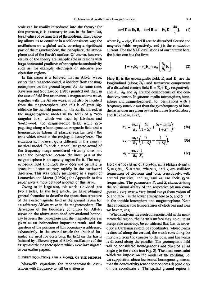
FIG. 1. TYPICAL HEIGHT PROFILES OF THE MAIN PARAMETERS
OF THE MODEL OF THE MEDIUM.
Roman numerals denote the layers which have been described in detail in the text : I-Earth ; II-atmosphere ; III-lower ionosphere ; IV-topside ionosphere ; V-mag- netosphere. The dash-dotted line represents the model value
of longitudinal conductivity CT,, = cc.
intermediate result, formulae are obtained which govern the penetration into the ground layers of sep- arate disturbance Fourier-harmonics, i.e. mono- chromatic oscillations, having a given horizontal wave vector which is arbitrarily oriented with respect to the meridian. When developing the analytic theory, we are using a realistic model of the vertical stratification of the ground layers. A typical vertical behaviour of the model parameters is given in Fig. 1. The particular form of the functions presented in it can be taken from both the experiment and some standard models. It is also essential that an arbitrary inclination of the geomagnetic field to the Earth’s surface is allowed for in this case.
The only important constraint which we impose on the model of ground layers is the assumption of their horizontal homogeneity. Incidentally, from simple physical considerations it is clear that such a homo- geneity is required only at a length of the order of a typical horizontal scale of the oscillation field (- 100 km). Horizontal inhomogeneities with a much larger
Field-induced oscillations of magnetosphere 531
scale can be readily introduced into the theory: for this purpose,_it is necessary to use, in the formulae, local values of parameters of the medium. This reason- ing allows us to consider in a selfconsistent way the oscillations on a global scale, covering a significant part of the magnetosphere, the ionosphere, the atmos- phere and of the Earth’s surface. Of course, however, results of the theory are inapplicable in regions with large horizontal gradients of ionospheric conductivity such as, for example, electrojets or intensive pre- cipitation regions.
In this paper it is believed that an Alfven wave, rather than magneto-sound, is incident from the mag- netosphere on the ground layers. At the same time, Kivelson and Southwood (1988) pointed out that, in the case of field line resonance, a magnetosonic wave, together with the Alfven wave, must also be incident from the magnetosphere, and this is of great sig- nificance for the field pattern on the Earth. Indeed, in the magnetosphere model in the form of a “rec- tangular box”, which was used by Kivelson and Southwood, the magnetosonic field, while pro- pagating along a homogeneous magnetic field and a homogeneous (along it) plasma, reaches freely the ends which simulate the conjugate ionospheres. The situation is, however, quite different in the axisym- metrical model. In such a model, magneto-sound of the frequency range considered virtually does not reach the ionosphere because the inner part of the magnetosphere is an opacity region for it. The mag- netosonic field amplitude there does not oscillate in space but decreases very rapidly in the earthward direction. This was briefly mentioned in a paper of Leonovich and Mazur (1989a) ; the Appendix to this paper gives a more detailed account of this issue.
Owing to its large size, this work is divided into two articles. In the first article, we have obtained general formulae to describe the space-time structure of the electromagnetic field in the ground layers for an arbitrary Alfvtn wave in the magnetosphere. The derivation of the boundary condition for Alfven waves on the above-mentioned conventional bound- ary between the ionosphere and the magnetosphere is given as an independent important result, and the question of the position of this boundary is addressed exhaustively. In the second article the obtained for- mulae are used for describing the field on the Earth induced by different types of Alfven oscillations of the axisymmetric magnetosphere which were investigated in our earlier papers.
2. INPUT EQUATIONS AND A MODEL OF THE MEDIUM
Maxwell’s equations for monochromatic oscil-
lations with frequency o will be written as
curl E = ikoB, curl B = - ikoE + q j, (1)
where k0 = o/c, E and B are the disturbed electric and magnetic fields, respectively, and j is the conduction current. For the VLF oscillations of our interest here, the latter one has the form
BO i = qE,, +alEl +Q,., By .
[ 1 (2) 0
Here B. is the geomagnetic field, El, and E, are the longitudinal (along B,) and transverse components of a disturbed electric field E = E,, +E,, respectively, and a*, cr+, and c,, are the components of the con- ductivity tensor. In gaseous media (atmosphere, iono- sphere and magnetosphere), for oscillations with a frequency much lower than the gyrofrequency of ions, the latter ones are given by the formulae (see G&burg and Rukhadze, 1975)
(34
(3b)
enOc 1 CII = F s,. (3c)
Here e is the charge of a proton, no is plasma density, S, = ~,/a~, Si = vi/Wi, where V, and vi are collision frequencies of electrons and ions, respectively, with neutral particles, and w, and wi are their gyro- frequencies. The parameters S, and ,Si characterizing the collisional ability of the respective plasma com- ponent, vary over a very broad range from values of S, and Si >> 1 in the lower atmosphere to S, and Si << 1 in the topside ionosphere and magnetosphere. Note that at comparable temperatures of electrons and ions we have v, << vi.
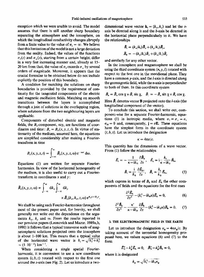
When studying the electromagnetic field in the near- terrestrial region, the Earth’s surface may, to quite an acceptable accuracy, be considered flat. Let us intro- duce a Cartesian system of coordinates, whose z-axis is directed along the vertical, the x-axis runs along the meridian from the equator to the pole, and the y-axis is directed along the parallel. The geomagnetic field will be considered homogeneous and directed at an angle x to the z-axis (see Fig. 2). The main constraint which we impose on the model of the medium, i.e. the supposition about horizontal homogeneity, means that the conductivity tensor components depend only on the coordinate z. The spatial ground region is

532 A. S. LEONOVXH and V. A. MAWR
b
FIG. 2. Tua MUTUAL POSITION OF THE THREE COORDINATE
SYSTEMS USED IN THIS PAPER: (X,&Z), (t,b,Z), (fl,JJ,l).
divided into several layers. Let us describe them briefly (see also Fig. 1).
(I) The Earth (z < 0). The Earth has isotropic conductivity, which means c,, = CT,, = erg, crH = 0. A typical value of conductivity is rather large: ~a = (lo’- 10”) SC’ such that most ofthe subsequent results remain unchanged when passing to the limit of an ideally conducting Earth : erg -+ co. The vertical dependence a,(z) has, as a consequence of the multi- layered structure of the Earth’s crust and mantle, a very complex character, but we shall confine ourselves to the simplest assumption CT* = const which permits us to take the non-ideal terrestrial conductivity crudely into account.
(II) The atmosphere (0 < z < H). The con- ductivity of this layer (and of all the above-lying ones) is described by formulae (3). The atmosphere provides a strongly collisional medium where S, >> 1 and $ s 1. The relationships (3) in this case yield
flil = trl = o,, (mu = a,/$, where a, = e2nofm,v,. We shall assume that a, = 0, i.e. we shall consider the atmosphere also to be an isotropic medium. Atmos- pheric conductivity grows upwards very rapidly, approximately exponentially with a typical scale of about S-10 km. In the lower part of the atmosphere, for the frequencies of our interest here, the inequality u, << 0/47c is satisfied with a large margin. The upper boundary of the atmosphere is defined by the con- dition S, N 1, which gives H = 80-100 km. Near this boundary cr, = IO’-lo6 s-’ and, hence, the inequality cr, D w/4a is fulfilled with a large margin. Note that the lowest ionosphe~c layer (D-layer) is included in the atmosphere here because the conducti~ty there is still isotropic.
(III) The lower ionosphere (25 < z < H-i-6). The collisional parameters there run through values equal to unity, at first S, at 90-100 km altitude and then S, at 120-140 km altitude. In this layer we shall assume al = up, where up is the Pedersen conductivity, the expression for which is given by formula (3a), in which one should put o/wi = 0. A maximum of Pedersen conductivity lies in a region where S, N 1. Hall con- ductivity is concentrated in a layer where the inequalit- ies S, < I and S, > 1 are satisfied. It may be identified with the mo~holo~cally distinguished .&layer. Typi- cal maximum conductivity values of the dayside iono- sphere are a,, = 3 - lo6 s- ’ and err = IO6 SC’. The thickness of the lower ionosphere, i.e. of a layer in which the Hall and Pedersen conductivities are con- centrated, is A _ 50-100 km. The longitudinal con- ductivity o,, _ ap/Se is much larger than crp and uH, and we shall assume that cr,, = co. Thus, the iono- sphere is a medium with sharply anisotropic con- ductivity.
(IV) The topside ionosphere (H+A < z < zA). In this case the plasma is nearly a collisionless one: S, CC 1 and S, << 1. The longitudinal conductivity is very large such that one is still more justified in assuming that Q,, = co. When vi << w, the decisive role in (3a) is played by the term with frequency. In this case
.w c2 c k: gL;= -*-T= -i----,
4n A 4n k, (4)
where it is designated : A = ~ol~4~is the Alfven velocity, and k, = w/A. In this layer cr, c 1~~1 and it will be assumed that Q~ = 0. The Alfven velocity involved in (4) varies in the layer under consideration in a very wide range ; it has a minimum value of 200- 300 km s- ’ in the F-layer and, while increasing rapidly, reaches a maximum of the order of lo4 km s-i at heightz,=(l-2)*103km.
(V) The magnetosphere (z > zA). The region above the Alfven velocity maximum will be considered to be the ma~etosphere proper. It differs from the topside ionosphere only in as much as the Alfven velocity there varies slowly, i.e. a typical scale of its variation is of the order of the field line length.
Let us make several remarks on the boundaries between the different layers. There actually exists only one sharp boundary, the Earth’s surface, where con- ductivity experiences a large jump. This is included in the model described here. Under real conditions there are no other sharp boundaries, and the layers insen- sibly shade into one another. In accordance with this, the parameters of the medium between the layers in our model change continuously ; but there is one
Field-induced oscillations of magnetosphere 533
exception which we were unable to avoid. The model assumes that there is still another sharp boundary separating the atmosphere and the ionosphere, on which the longitudinal conductivity changes abruptly from a finite value to the value of o,, = co. We believe that this limitation of the model is not a large deviation from the reality. Indeed, the values of the functions Q,,(Z) and a,(z), starting from a certain height, differ in a very fast increasing manner and, aheady at 1% 20 km from that, the value of cr,, exceeds Q,, by several orders of magnitude. Moreover, it appears that the crucial formulae to be obtained below do not include explicitly the position of this boundary.
A condition for matching the solutions on sharp boundaries is provided by the requirement of con- tinuity for the tangential components of the electric and magnetic oscillation fields. Matching on smooth transitions between the layers is accomplished through a join of solutions in the overlapping region, where solutions from the two neighbouring layers are applicable.
Components of disturbed electric and_ magnetic fields, the &component, say, are functions of coor- dinates and time : B, = B,.(.x, y, z, f). In virtue of sta- tionarity of the medium, assumed here, the equations are simplified ~onside~bly after making a Fourier- transform in time
Equations (1) are written for separate Four-i&- harmonics. In view of the horizontal homogeneity of the medium, it is also useful to carry out a Fourier- transform in coordinates x and y :
xiJ (k X k z o)e*xX+ik*y. XV y* 9
We shall be using such Fourier-harmonics throughout most of the present paper and, for brevity, we shall generally not write out the dependence on the argu- ments k,, k, and o. From the results reported in our previous papers (Leonovich and Mazur, 1989a,b, 1990) it follows that a typical transverse scale of mag- netospheric solutions projected onto the ionosphere is about I-100 km. This means that a typical value of the horizontal wave vector is k, = dm N (l-lo- *) km- ‘.
When considering a single spatial Fourier- harmonic, it is convenient to use a new coordinate system (t, 6,~) rotated with respect to the first one around the z-axis (see Fig. 2). Let us introduce a two-
~mensional wave vector kt = (k,,k,) and let the r- axis be directed along it and the b-axis be directed in the horizontal plane perpendicularly to it. We have the relationships
and similarly for any other vector. In the ionosphere and magnetosphere we shall be
using the third coordinate system (n, y, I) rotated with respect to the first one in the meridional plane. They have a common y-axis, and the I-axis is directed along the geomagnetic field, while the n-axis is ~~ndi~~ar to both of them. In this coordinate system
B,=BXwsx+BZsinx, B,, = -B,sinX+B,cosX.
Here B, denotes vector B projected onto the f-axis (the longitudinal component of the vector).
To conclude this section, we shall write out, com- ponent-wise for a separate Fourier-harmonic, equa- tions (1) in isotropic media, where or = o, = o, or, = 0 and, consequently, j = crE. These equations have the simplest form in the coordinate system (t, b, z). Let us introduce the designation
K = 4rRr/&.
This quantity has the dimensions of a wave vector. From (1) follow the relationships
which express in terms of Bb and Eb the other com- ponents of fields and the equations for the first ones
2 - (kf -ik,lc)&, = 0, (61
a’& K’ a&, - -__ --(kz-ik,%)& = 0.
az2 K-iko az (7)
3. THE EIXCI’ROMAGMTIC FIELD IN THE FARTH
Let us introduce the designation rep = 4nu.&. By taking account of the terrestrial homogeneity pro- posed here, we reduce equations (6) and (7) to the form
&k;& = 0, &k,2&, = 0,
where it is designated
kg = dkx
534 A. S. LEONOVXXI and V. A. MAZUR
and the radical sign is chosen such that Re kg > 0. In limiting cases we have
kg = I
k,, kf >> korcg,
j(k,rc,) I”, k: << korcg,
where j= e-'n14 = (1 -i)/,/?. Bearing in mind the typical limits of variations of the parameters k, = 1-10-2km-i, o = 10-2-10-‘s- ‘, and Gg = 108-10’o s- r, it is easy to see that both limiting cases are real- izable. The typical range of possible values of jk,] = l-10-2km-‘.
The solutions of equations (6) and (7), which are bounded when z c 0, have the form
$(z) = &(O) ekg”, &(z) = Z&,(O) ek8”. (ga)
From this and from the equalities (5), we have
B,(z) = &(O) eks’, $(z) = $(O) e+, (gb)
with
B;(O) = i$&(O), &(O) = -2&(O). (9) 0
These last relationships will be used as the boundary conditions for the solution in the atmosphere.
Thus, the oscillation field decreases exponentially deep into the Earth with a typical scale Zp = (Rek,)- ‘. If k,rc, is larger than or comparable with k:, this decrease is attributable to spatial oscillations as is the case in the classical problem of the skin layer.
Using the WKB approximation it is easy to obtain a solution for the case of a weakly inhomogeneous Earth, whose inhomogeneity scale is much larger than I,. In this case the results remain almost unaltered because the solution is concentrated near the ter- restrial surface on a scale Z8 where conductivity is assumed to change little.
In the case of a very high conductivity of the Earth, when kotcg >> k:, from (9) follows
and in the limit JC~ -+ co, as should be the case, &(O) = $(O) = 0.
4. THE ELECTROMAGNETIC FIELD IN THE
ATMOSPHERE
Atmospheric conductivity is much smaller than the Earth’s conductivity and the inequality k: >> koic, is valid throughout the atmosphe~c height. Therefore, the term ik,lc, in equation (6) can be regarded as a disturbance. In the main approximation we have
This equation, together with the equality (5) and the boundary condition (9), leads to the following solution :
&(z) = B,(O) (
cash k,z+ 5 sinh k,z )
, g
$(z) = &(O) (
cash k,z+ 5 sinh kg), (10) t
with
&i,(O) = -i(k,/k,)&(O).
From this, in particular, follows
B,(O) = B,(N) (
cash k,H+ 2 sinh k,H -1
> (11)
8
and
B,(H) = i?&(H), (12) 0
where it is designated
n _ 1 + (k&l tanh k,H
tanh k,H+k,/k, *
The equality (12) will be used subsequently as the boundary condition for a solution in the ionosphere.
In the next order of perturbation theory one may take account of the term ik,tc in equation (6) and obtain corrections for the solution (10) and the relations~p (12). Small corrections to the functions B, and $ are of no practical concern. The correction to the relationship (12) will, ultimately, transform into a corresponding correction to the boundary condition for an Alfven wave at the upper boundary of the ionosphere and will define that part of the damping decrement, which is connected with dissipation in the atmosphere. This part consists of only a negligible portion of the total decrement, which is determined mainly by the dissipation in the ionospheric Pedersen layer. Therefore, in equation (6) one can totally neglect the atmospheric conductivity effect.
Quite a different situation applies to equation (7). The term iko& in the last bracket of this equation can also be neglected, but the factor rc:/(rc.-ik,), caused by the inhomogeneity of atmospheric conductivity, plays the decisive role. Let us designate
S=i-& B 0
and let us rewrite equation (7) as
&-2Spb-k2& = 0. t
Field-induced oscillations of maguetosphere 535
A typical scale of variation of the function S(z) is of the order of the atmospheric height H. Assuming that the scale of variation of the solution is much smaller, we shall seek it using the WKB method. Setting B b = exp Y(z), we get
Y’2+1”-2SY’-k~ = 0.
We seek the function Y by the successive approxi- mation method: Y = Y,,+Y, ++. . . In the main order
‘rb’ -2SY0 - k: = 0.
This quadratic equation has two roots :
Y; = q,,* = s&d=.
In the next order, for each of them, we obtain the equation
2(q-S)Yy; +(I’ = 0,
from which it follows that
I, = - ;In(q’+k:).
On the basis of these results it is easy to write a general solution for&(z). It depends on two arbitrary constants. Using relationship (5), this solution can yield the expression for j?,(z). After that, the boundary condition (9) makes it possible to interconnect the arbitrary constants and to express them in terms of a single one. The result can be represented as
(134
UW
When deriving expressions (13), we have neglected the extremely small value of k,k,/k,rc, as compared with unity.
In the lower part of the atmosphere, where IC, << ko, the value of S is very small and q 1,2 = + k,. From (13) it then follows
$(z) = C sinh k,z, I&,(z) = i(k,/k,)C cash k,z.
(14)
In the upper part of the a~osphere the inequality rc, >> k. is satisfied (with a very large margin). There- fore S = 1/2h, where
h(z) = ~~tz)~~~tz) = cr,tzwm is a typical scale of variation of conductivity. As has already been stated, when describing the model of the medium, if it is sufliciently small, h = 5-10 km (and we shall assume that k,h << 1) then
q1 = ;+kfh, qZ = -k:h.
Note also that
where it is designated
Since Re Q % 1, near the upper boundary of the atmos- phere, only the first terms can be retained in (13). Then
E&r) =&(H)exp(-k?%hdz’), (Isa)
~(4 h(z) B,(z) = B,(H) - ~ WV h(H)
exp( -k:rh dz’),
and
i?;(H) = C[k,I2x,(H)] ‘/’ eQ-11114,
&(H) = -C[~,K,(H)/~]*‘~~(H)~Q-‘“~~. (16)
From relationships (16) it follows that
B,(H) = - x,(H)h(H)$(H).
The coefficient ~=(~h(~) involved here is of the same order of magnitude as the atmospheric conductivity- induced correction to the coefficient i&/k, in equality (12). For the same reason, as in the case of neglecting this correction, we must also neglect the coefficient rcah. Thus, in the approximation we have adopted
B,(H) = 0. (17)
In order to avoid a misunderstanding, we wish to note that the numerical value of the coefficient
IE,(H)htH) N lo3 seems to be large; but, as follows from (12), the representative value of the coefficient of pro~~ona~ty between the electric and magnetic field k,/k, N 105-lo’, i.e. by several orders of mag- nitude larger.
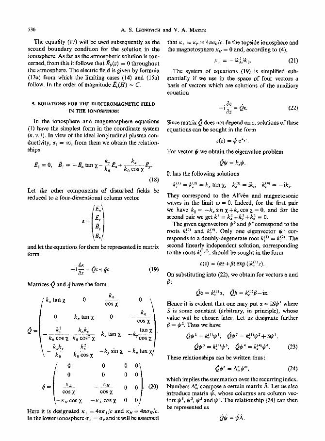
536 A. S. LE~NOVICH and V. A. MAZUR
The equality (17) will be used subsequently as the second boundary condition for the solution in the ionosphere. As far as the atmospheric solution is con- cerned, from this it follows that&(z) = 0 throughout the atmosphere. The electric field is given by formula (13a) from which the limiting cases (14) and (Isa) follow. In the order of magnitude $(H) N C.
5. EQUATIONS FOR THE ELE~ROMAGNRTIC FIELD IN THE IONOSPHERE
In the ionosphere and magnetosphere equations (1) have the simplest form in the coordinate system (n, y, I). In view of the ideal longitudinal plasma con- ductivity, u,, = co, from them we obtain the relation- ships
E,, = 0, B,, =
08)
Let the other components of disturbed fields be reduced to a four-dimensional column vector
and let the equations for them be represented in matrix form
a& -i- = &E+@.
aZ
Matrices $ and 4 have the form
ko 0 -
cos x
k,tanx 0
k, tan %
kk _ x2 k,’
ko ~ -k,,sinX -k, k, cos x
1 0 0 0 0 0 0 0 0 \
(j= KL
i
uff -- -__ 0 0 * (20) cos x cos x
--u,eos~ -U,COS~ 0 0 i
Here it is designated ICY = 4ncrJc and lcII = 4~cr,jc. In the lower ionosphere c1 = ep and it will be assumed
that fcI = or = 47&c. In the topside ionosphere and the magnetosphere IC* = 0 and, according to (4),
KA = - iki/ko. (21)
The system of equations (19) is simplified sub- stantially if we use in the space of four vectors a basis of vectors which are solutions of the auxiliary equation
a& -i- = &E. aZ
Since matrix Q does not depend on z, solutions of these equations can be sought in the form
E(Z) = + e’+.
For vector $ we obtain the eigenvalue problem
& = k&.
It has the following solutions
kit) = kz2) = k, tan x, kz3) = ik,, kz4) = -ik,.
They correspond to the Alfven and magnetosonic waves in the limit w = 0. Indeed, for the first pair we have k,, = -k, sin x+ k, cos x = 0, and for the second pair we get k2 = k: + k,’ + k,’ = 0.
The given eigenvectors II/’ and $“ correspond to the roots ki3) and ki4). Only one eigenvector rl/’ cor- responds to a doubly-degenerate root kz’) = ki2). The second linearly independent solution, corresponding to the roots ki’**), should be sought in the form
s(z) = (az+B) exp(ik’,‘)z).
On substituting into (22) we obtain for vectors GI and
B:
ou = ki’)cI, &/I = ki’)j?-ix.
Hence it is evident that one may put CI = iS$’ where S is some constant (arbitrary, in principle), whose value will be chosen later. Let us designate further p = rlf’. Thus we have
&’ -_ ki’f$‘, &’ = k~l)~*+~~‘,
&II/’ = k(3)$3 z >
&J/4 = ,@4’$4 I . (23)
These relationships can be written thus :
Qtp = l&p, (24)
which implies the summation over the recurring index. Numbers A; compose a certain matrix i% Let us also introduce matrix 5, whose columns are column vec- tors J/‘, tff’, $J~ and $“. The relationship (24) can then be represented as
&$ = l&X.
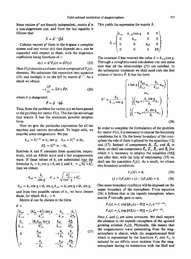
Field-induced oscillations of magnetosphere 531
Since vectors +” are linearly independent, matrix $ is a non-degenerate one, and from the last equality it follows that
Column vectors $” form in the 4-space a complete system and any vector c(z) that depends on z, can be expanded with respect to them, with the expansion coefficients being functions of z :
E(Z) = lpF,(z) = $F(z). (25)
Here F(z) denotes a column vector composed of F,,(z)- elements. We substitute this expansion into equation (19) and multiply it on the left by matrix $- ‘. As a result we obtain
aF -iaz = ib+pF,
where it is designated P’ = ko
P = $-‘@J. k,, cosx
Thus, from the problem for vector E(Z) we have passed to the problem for vector F(z). This has the advantage that matrix fi has the maximum possible simplest form.
Now we give the particular expressions for all the matrices and vectors introduced. To begin with, we describe some designations. We put
kzA = ki’,‘) E k, tan x, krF = kj3) = ik,,
k$ = kc4) E Z -ik t’
Symbols A and F associate these quantities, respec- tively, with an Alfven wave and a fast magnetosonic wave. If these values of k, are substituted into the formulae k, = k, cos x + k, sin x and k, = Jm, then we obtain
In order to complete the formulation of the problem for vector F(z), it is necessary to impose the boundary conditions for it. On the lower boundary of the iono- sphere the role of them is played by the equalities (12) and (17). Instead of components &, & and’ & in them, we shall use components &,, E,,, i$,, and 8. [for which it is necessary to employ the equalities (18)] and after that, with the help of relationship (25) we shall use the quantities F,,(z). As a result, we obtain two boundary conditions
k knA = 2 k
cosx’ IA =
knF = k, cos x + ik, sin x, k,, = k, cos x + ik, sin x,
and from two possible values of kl we have chosen those, for which Re kL > 0.
Matrix $ can be chosen in the form
5=
k nA
k IA
k Y
k IA r 0
0
(kk - k,Z) tan x - k:A
2k,k,, tan X - k:,
k II* -
ko
k -2 k,
k _Y k IF
k “F k IF
k -i2 ko
k -i-T!!? k,
k _Y k%
k%
kf,
-I
k i-l: . ko
k& i- k,
(27)
This yields the expression for matrix A :
The constant S has received the value S = klA/cos x. Through a straightforward calculation one can make sure that all the relationships (23) are satisfied. In the subsequent treatment we shall need only the first column of matrix p. It has the form
F,(H) = 0, (29)
(n+l)F,(H)+(L- l)F4(H) = 0. (30)
One more boundary condition will be imposed on the upper boundary of the ionosphere. From equation (26) it follows that in the topside ionosphere, where matrix B virtually goes to zero,
F,(z) =f3 exp [ikrF(z-EZ)] =f, e-kl(Z-H),
F4(z) = f4 exp [ik$(z-_H)] = f4 ek@-“).
Heref3 andf, are some constants. We shall require the absence in the topside ionosphere of the upward growing solution F4(z). Physically, this means that the magnetosonic wave penetrating from the mag- netosphere is absent, while the magnetosound field which is represented by the functions F3 and F4, is induced by an AlfvCn wave incident from the mag- netosphere during its interaction with the Hall and

538 A. S. LE~NOVICH and V. A. MAZUR
Pedersen ionospheric Iayers. The field of such a mag- netosound must decrease upwards. On the upper boundary we put
F,$(z*) = 0. (31)
Thus, for the system of four homogeneous equations (26) with four unknown functions F,,(z) there exist three homogeneous boundary conditions (29)-(31). Consequently, the solution is determined up to a fac- tor common for all functions F,,. Its value is then determined, when matching with the magnetosphere solution, by the Alfvbn wave amplitude.
6. SOLUTION FOR THE ELECTROMAGNETIC FIELD IN
THE IONOSPHERE
We shall solve the problem for vector F(z), by using a modification of perturbation theory based on the smallness of matrix 3. The physical meaning of this smallness has been pointed out in the Introduction, namely that the frequency of the oscillations con- sidered must be much less than ionospheric eigen- frequencies. Mathematically corresponding con- straints will be formulated below.
When solving the system (26), it is convenient to introduce the new functionsf,(z) defined by the equal- ities
F,(z) = f”(z) exp [ik(“)(z-H)]. I (32)
Let us try, at first, to apply a standard perturbation theory. In its zero order, by assuming $ = 0, we have the problem
f; = -i(klA/cos x)f2, f; =f; =Sh = 0,
f*(H) = 0, (n+l)f~(H)+(1-l)f,(HT) = 0,
.f4(%> = 0.
It has the solution fi = f = const, f2 = f:, = f4 = 0. By calculating, then, a first-order correction to this solution, it is easy to see that the correction to the function f, turns out to be not small compared with f, itself. The point here is that in the Pedersen layer of the lower ionosphere the function ft , while chang- ing little in magnitude, alters significantly its deriva- tive, and in the topside ionosphere, while obeying the equationf’; = 0, it changes linearly with coordinate z and, owing to the high altitude of the ionosphere zA alters its value significantly. Thus, a standard per- turbation theory is inapplicable; but on the basis of the same formulae one can draw the conclusion that the inequalities
Ifill I&L Ifal << Lfil
hold throughout the entire ionosphere. It is this
assumption that will form the basis for our varient of perturbation theory. It allows us to simplify con- siderably system (26), by retaining in the small term PF only the main component P’F, = P ‘f, exp [ik_,(z- H)]. After that, the first pair of equations of the system splits out, and we begin our treatment by considering it.
We have the following equations
W)
y2 = - k. ka ~0s x Jclfi, Wb)
and the boundary condition
five = 0. (34)
We introduce the constant f = f, (H) which will play the role of a common factor for the entire solution. Besides, we denote
s W+A
KP," = X,&Y-i-A) 5 KP,H(Z) d.z. x
Note that Kp., = 4nC,n/c, where
s H-eA
&V, = ~P,H (~1 dz H
are the integral Pedersen and Hall ionospheric con- ductivities.
The right-hand side of equation (33b) contains the term rcI(z) f, (z). In the lower ionosphere ICY z IC,, and the functionf, (z), as will be shown in the following, changes little : f, (z) fi: f. In the topside ionosphere the value of (21) for ICY is small and, by neglecting for the time being its difference from zero, one can see that in the entire ionosphere it is possible to put Kl(z) f, (z) z Ice(z) f. From (33b) and (34) it then fol- lows that
fit.4 = -f ko
k,, ~0s x X,(z).
In the topside ionosphere, when z > H+ A, this equal- ity yields
fi(4 = -f kof&
kiA cos 71.
Here the function fz(z) is a constant. From the obtained expressions it is apparent that for the
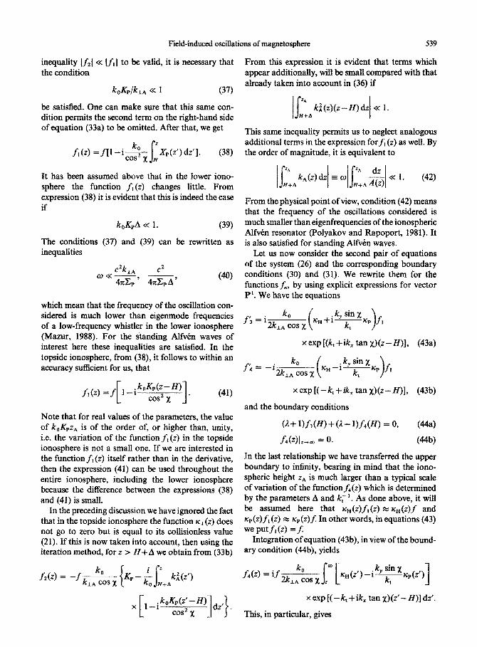
inequality If21 c If,] to be valid, it is necessary that the condition
k&/k,, << 1 (37)
be satisfied. One can make sure that this same con- dition permits the second term on the right-hand side of equation (33a) to be omitted. After that, we get
f,(z) =f[l-i& (38)
It has been assumed above that in the lower iono- sphere the function f,(z) changes little. From expression (38) it is evident that this is indeed the case if
koKPA << 1. (39)
The conditions (37) and (39) can be rewritten as inequalities
(40)
which mean that the frequency of the oscillation con- sidered is much lower than eigenmode frequencies of a low-frequency whistler in the lower ionosphere (Mazur, 1988). For the standing Alfven waves of interest here these inequalities are satisfied. In the topside ionosphere, from (38), it follows to within an accuracy suf5cient for us, that
f,(z) =fll-ik0z$,8)]. (41)
Note that for real values of the parameters, the value of koKPz, is of the order of, or higher than, unity, i.e. the variation of the functionf,(z) in the topside ionosphere is not a small one. If we are interested in the functionf,(z) itself rather than in the derivative, then the expression (41) can be used throughout the entire ionosphere, including the lower ionosphere because the difference between the expressions (38) and (41) is small.
In the preceding discussion we have ignored the fact that in the topside ionosphere the function rcI(z) does not go to zero but is equal to its collisio~ess value (21). If this is now taken into account, then using the iteration method, for z > H+A we obtain from (33b)
f*(z) = -f k,
ku ~0s x k:(f)
From this expression it is evident that terms which appear additionally, will be small compared with that already taken into account in (36) if
IS ZA
k&)(z-H) dz cc 1. H-&4.
This same inequality permits us to neglect analogous additional terms in the expression forf, (z) as well. By the order of magnitude, it is equivalent to
From the physical point of view, condition (42) means that the frequency of the oscillations considered is much smaller than eigenfrequencies of the ionospheric Alfvbn resonator (Polyakov and Rapoport, 1981). It is also satisfied for standing Alfven waves.
Let us now consider the second pair of equations of the system (26) and the corresponding boundary conditions (30) and (31). We rewrite them for the functions f., by using explicit expressions for vector P’. We have the equations
S; = i
x exp [(k, + ik, tan x)(z - H)], (43a)
xexp[(-k,+ik, tanX)(z-H)], (43b)
and the boundary conditions
(A+ l)f,(H) + (A- l)&(H) = 0, (44a)
s4(z)l,+, = 0. (44b)
In the last relationship we have transferred the upper boundary to infinity, bearing in mind that the iono- spheric height z, is much larger than a typical scale of variation of the functionf,(z) which is determined by the parameters A and k; ’ . As done above, it will be assumed here that rcu(z)f, (z) x ICKY and rcp(z)fi (z) E r+(z)S. In other words, in equations (43) we putfr(z) =$
Integration of equation (43b), in view of the bound- ary condition (44b), yields
h(z) = if k sinx
rcu(z’)-i k y QZ(z’) t 1
Field-indu~ oscillations of m~~etosph~re 539
xexp[(-k,+ik, tanx)(z’--H)]dz’.
This, in particular, gives

540 A. S. LEo~ovrcn and V. A. MAZUR
fd(H) = if 2k,AkEosX Kn-ik$!%& , (45) t 1
where it is designated
I
a, %,n = tcp,n(z) exp [(-k, +ik, tan x)(2-H)] dz.
H
(46)
From the equality (44a), by using an explicit ex- pression for the quantity /2, we obtain
f3(H) = -
Finally, integration of equation (43a) yields
r&z’) 1 x exp [(k, +ik, tan x)(z’--H)] dz’.
In summarizing the result of this section, we write out the expressions for all functions F,,(z) = fn(z) exp [ik$)(z--H)] :
F,(z) =f l-i ko&(z-HI
co2 x 1 x exp [ik,(z--H) tan x], (48a)
F,(z) = -f k,&(z)
ku ~0s x exp ]ik,(z- H) tan x], (48b)
F3(z) =: f,(H)e-'~('~)+i~-~~s~ IA
f X S[
IcH(z’)+i k sin x k- ?+(z’)
H k, 1 x exp [(k, + ik, tan x) (z’ - H)] dz’, (48~)
Fe(z) =if ko ek,(--ff)
2k,, cos x
X nn(z’)-i k sin x y ?ce(z’)
k, 1 x exp [(-k, + ik, tan x)(z’ - H)] dz’. (48d)
7. MATCHING OF SOLUTIONS IN THE IONOSPHERE
AND MAGNETOSPHERE AND THE BOUNDARY
CONDITION FOR ALFVEN WAVES
From the formulae of the preceding section it fol- lows that in the topside ionosphere
F,(z) = f [
1 -i k”zo$yH) 1 elk,(z-w)ta” x ,
Fz(z) = -fEok e “,(2-H) tan x , (4%
IA
F,(z) -+ 0, Fd(Z) + 0. (50)
These relationships are also equally applicable in the lower magnetosphere, merely because the boundary between these layers is a sufficiently arbitrary one. From relationship (SO) it follows that a four-vector of el~troma~etic field is given by the expression
a(z) = $‘;c,(z)+@Fz(z). (51)
Using explicit expressions for vectors I//’ and lfi2 we then have
Here we have designated
B, = -fK&os x.
The quantity BA is the oscillation amplitude of a dis- turbed magnetic field of an Alfvtn wave in the topside ionosphere and in the lower magnetosphere. As one can see, in these layers it is a constant. The last equality can also be written as :
f = -BAcosx/&., (53)
by expressing the constant f in terms of the Alfven wave amplitude. The electric field of the Alfven wave is given by the same expression (51). In view of relationship (53) and the inequalitity lE;l CC IF, 1, we have
$(z) = iBA $ IA
X
E,,(z) = iBA$ IA

Field-induced oscillations of magnetosphere 541
In our previous papers (~novich and Mazur, 1989a,b, 1990) we have used the boundary condition for Alfvkn waves on the ionosphere, without giving its derivation. We shall do this in the present paper because all formulae required for this have been obtained. The desired boundary condition is a relationship between the derivative of a disturbed field and itself on the upper boundary of the ionosphere. This condition has the most suitable form if the derivative is taken along a field line
a a z=cos~.,+ik,sin~.
For calculating this derivative, the accuracy, to within which the expressions (52) are obtained, is insufficient. From them it follows that in the topside ionosphere and in the lower ma~etosphere, and also when z = z,, we have
aBn,y= a1 O*
This equality can be considered to be a zero approxi- mation for the desired boundary condition. It means that the magnetic field of the wave has an antinode on the ionosphere.
In order to obtain it to a desired accuracy, it is easiest to proceed from equations (33) which in the topside ionosphere and in the lower magnetosphere have the form
From the equality (51) we have B,, = (k,,/k,)F,, $ = (-k,,/k,)F,. By differentiating these equalities with respect to i and using the second equation of (56), we obtain
aB,_k,kiF a&z k,kiF --- _ --- al k,, k. I’ ar-- koko ”
(57)
We substitute here the expression (48a). Using also relationships (52) and (53) we obtain
a& _ al
and this is, in fact, the desired boundary condition for matching the solutions in the topside ionosphere and in the lower magnetosphere. Only the question as to where the boundary between these layers should be drawn, remains unclear, especially as the function ki (z) changes very rapidly in the topside ionosphere. In principle the answer is clear, namely that the boundary can be established at any height in the layers involved. The strong dependence of ki on z must not affect the
results of appli~tion of the boundary condition. In order to prove the last statement, we obtain
the equation for Bny. To accomplish this, we divide equations (57) by ki, differentiate them with respect to I and use the first equation of (56). As a result, we
get
This equation coincides with equations for Alfv& waves in the magnetosphere given in our previous papers if the dispersion effects are neglected in them and if attention is confined to considering such a region in which the geomagnetic field can be con- sidered homogeneous. Let us integrate equation (59) along a field line from point I0 to point !, by assuming that both of them lie in the topside ionosphere or in the lower magnetosphere. This means that the distance between them is much less than the wavelength such that the functions &,? can be considered constants. We obtain
This equality totally agrees with (58) if it is taken into consideration that during the motion along the field line 1 -lo = (z - zo)/cos x. It permits us to transfer the boundary condition imposed at point lo, to any other point 1 on a given field line. It is clear that the solution must not change due to such a transfer.
Thus, the position of the boundary z = z, is deter- mined by considerations of convenience. It is appro- priate to choose it as low as possible but such that above it the function A(z) changes slowly. This approximately corresponds to the height of the maximum of the function A(z) (see Fig. 1). Otherwise, the ma~etosphe~c part of the field line would include portions with sharply different scales of variation of A, which would considerably complicate the solution of the equation for Alfvkn waves in the mag- netosphere.
The two terms in brackets on the right-hand side of the equality (58) play a substantially different role. Both of them are, in a sense, small. Since the functions BRy describe an Alfvkn wave, a typical value of the derivative a&,/al N k,$,y. The two terms concerned are small compared with this value, which agrees quite well with the zeroth-order approximation (55). The second term is, in absolute value, of the order of or even greater than the tint one, but since. it is real, its role is unimportant. Taking it into account in the boundary condition leads to a small change of the standing wave frequency which is of no practical con-

542 A. S. LJZONOVICH and V. A. MAZUR
tern. The first term, however, plays a fundamen~iy important role by determining the standing wave damping decrement due to the dissipation in the iono- sphere; therefore only it will be retained. As a result, the boundary condition can be written as
Note that in the equality it is easy to perform an inverse Fourier transform in k, and kY and to pass to the functions &,, the boundary condition for which has exactly the same form.
It should be pointed out that the boundary con- dition of the form (60) for the case of a vertical geo- magnetic field (x = 0) was obtained earlier for a sim- pler model of the medium in many papers (see reviews by Lyatsky and Maltsev, 1983 ; Southwood and Hughes, 1983). Our result means that the boundary condition virtually retains its form, despite the sig- nificant complication of the model (s~cifically, 71 + 0 and taking into account the presence of the topside ionosphere) and the treatment of waves with arbitrary k, and k,.
8. THE RELA~ONSHIP BETWEEN
ELECTROMAGNETIC FIELDS ON THE LOWER
BOUNDARY OF THE MAGNETOSPHERE AND ON THE
EARTH’S SURFACE
First of all, we shall obtain the relationships relating values of fields on the upper and lower boundaries of the ionosphere. Formulae for fields on the upper boundary have been obtained in the preceding section. From the equalities (34), (38) (45) and (47) as well as from the relationship (53) it follows that on the lower boundary
F,(H) = - FBA, P
F,(H) = 0,
ko k -k F,(H) = i--s---e
2k,, kg + k,
On substituting these values into formula (25) one can obtain expressions for the components $(H), E?(H), &,(H), and &(H) and using them, in view of the equalities (18), horizontal components of fields are obtainable. Simple, though cumbersome, calculations give
k, B,(H) = jy
cash k,H+ (k~/k~) sinh k,H e_k,H
IA 1 +W,
BA,
k0 &(H) = -ic
sinh k,H+ (k,/k,) cash k,H e_k,n
IA 1+ k/k,
B,(H) = 0. (61)
It is easy to see that these expressions satisfy the boundary conditions (12) and ( 17). Finally, from for- mulae (61) and from the results of Section 4 it follows that on the Earth’s surface
-k,H
- - B
A, W’)
Et(O) = 0, B,(O) = 0. (624
The results obtained, in total, solve the problem of the electromagnetic field induced in ground layers by an Alfven wave incident from the magnetosphere, provided that the wave is a separate Fourier-harmonic in time and in horizontal coordinates -exp (ik,x + ik,,y -iwt). Indeed, formulae (48) and (25), together with the equality (53), define the electromagnetic field in the ionosphere and in the lower ma~etosphere, formulae (lo), (ll), (13) and (16) together with (61) or (62), define the field in the atmosphere, and for- mulae (8) and (62) define the field in the Earth. By ~rfo~ng an inverse Fouler-tmnsfo~ in k,, k, and w, one can obtain the electromagnetic field dis- tribution in ground layers for an Alfven wave with an arbitrary space-time structure. We have accomplished this procedure for the field on the Earth’s surface, i.e. the most important case for practical purposes.
Let us limit our attention to the case of a highly conducting Earth, k,/k, -+ 0. From the relationships

Weld-induced oscillations of magnetosphere 543
(62) and (52) it follows that
&(k,, k,, 0, o) = cos x.
- Rkx, k,) - $tk,, k,, zA1d, Wa)
Bl,(k&k’d = -B(k,,k,)‘B,(k,,k,,zA,w),
(63b)
&(kx, k,, 0, co) = i ~ “k’ ky) [k,&(k,, k,,, z,, co) 8
Here
-kx ~0s x&k,, k,, ZA, @)I- (63~)
&k,, k,) = (‘ k sin x & 2 -i+ -
P t 4
xexp[-k,H-ik,(z,-Ei)tanX]
k,, sin x a&z) -i-
k, @P(Z) 1
xexp[-k,z+ik,(z-z,,)tan~]dz. (64)
Bearing in mind that the functions (~~(2) and (~~(2) are subs~ntially different from zero only in the lower ionosphere, integration over z formafly extends to the entire interval (0, co). As a result, it becomes apparent that these formulae lack the dependence on height H: i.e. an artificial boundary between the atmosphere and ionosphere.
Results of an earlier work devoted to an analytic investigation of the passage of the Alfven wave field to the earth through a ho~zon~lIy-homo~neous ionosphere, are particular cases of formulae (63) and (64). In one ofthem it is assumed that the geomagnetic field is a vertical one, x = 0, and the horizontal wave- length of the disturbance is much larger than the typi- cal thickness of the ionospheric conducting layer, k,A CC 1 (Hughes and Southwood, 1976a). Then
R(k,, k,,) = 2 e-V’. P
In another particular case the geomagnetic field is assumed inclined, x. # 0 but inde~ndent of the coor- dinate y (i.e. it is assumed that k, = 0) and also the condition k,A CC 1 is supposed (Hughes, 1974). In this case
R(k,,O) = $exp[- jk,iN---ik,x,l, (65b) P
where it is designated JC, = (2*-H) tan x. Inci- dentally, formula (65a) can be considered the par- ticular case of formula (Mb) because when x = 0 the horizontal wave vector kt can, without loss of gener- ality, be directed along axis X.
The conditions adopted when deriving the relation- ships (65) place considerable constraints on the possi- bilities of applying them to the real oscillations. The requirement k, = 0 forces one to consider only toroidal (or close to them) oscillations of the mag- netosphere. The condition k,A << 1 is extremely bur- densome. In connection with this, we want to note that the presence of the factor exp (- k,H) in formulae (65), which represents the field attenuation on the Earth for short-wavelength oscillations with kt & Ii- ‘, is, in fact, an excess of accuracy. The point here is that the parameters A and H are the values of the same order of magnitude ; therefore, the condition k,A << 1 simultaneously means also k,H << I. Thus, formulae (65) should be written in a still simpler form
g = $exp(-ikXx& P
but this expression is inapplicable for transversally- small-scale oscillations.
The general expression (64) we have obtained is free from these limitations. When k,A 3 1, the value of the function R(k,, k,,) is not determined only by integral conduotivities but depends substantially on the profile of the functions oH(z) and ~~(2). Besides, for waves with k,, # 0 (and when x # 0), in the expression for the function J?(k,, k,) there appears a fundamentally new term which shows that the penetration of an Alfvkn wave to the Earth can be due not only to Hall conductivity but also to Pedersen conductivity.
Let us perform in formulae (63) an inverse Fourier- transform in k,, k,, and o. We denote
Then
x fF(k,, k,) e*xc+*ytl. (66)
&(x, y, 0, t) = cos x. dy’
x R(x-x’,y-y’)B&‘,y’,zA,t), (674
co
B&c, y.0, t) = - s s
m
dx’ dy’ -03 --m
xR(X--x’,y-Y’)B,(~‘,y’,zA,t), Wb)

544 A. S. LE~NOVICH and V. A. MAZUR
We shall not give here the more unwieldy expression for B,(x, y, 0, t). By taking integrals over k, and k, in (66), we obtain a relatively simple expression for the nucleus of integral transformations :
R(& ‘11 = & P
s cc z(7H (z) + qcp (z) sin x
X ___. ~-
o [z2+(5+(z-zA)tanx)2+q213’2 dz. (68)
It is easy to see that exactly the same formulae also occur for Fourier-transforms in time &,(x, y, z, 0). Basically, formulae (67) and (68) solve the problem of the space-time structure of the oscillation field on the terrestrial surface if it is known on the lower boundary of the magnetosphere. They also yield simple particular cases as obtained in the above- cited references. These particular cases are to the same extent limited compared with the general relationship (68) as are the expressions (65) compared with (64).
The nucleus of integral transfo~ation R(x--n’, y-y’) in formulae (67) can be treated as a dis- turbance on the ground produced by a source concentrated in the magnetosphere on one field line passing through point x’, y’ at the ionospher~mag- netosphere interface, i.e. at height z = z,,. A quali- tative idea of this function may be obtained, by assuming that the thickness of the layer in which the Hall and Pedersen conductivities of the ionosphere are concentrated, is much smaller than the height of an isotropic atmosphere : A << H. From (68) it follows that
R(&q) =& H$+qsinx P
x[~z+(~-(z~-~)~nx)2+~2]-3’z. (69)
This expression can be applied in formulae (67) if a typical scale of the functions B,,u in coordinate x is much larger than A tan x (which is far from being always satisfied). A typical scale of the function R(& q) in both variables is of the order of the atmos- pheric height, and this is particularly obvious for expression (69). This means that small-scale details in the oscillation field distribution at the lower edge of the magnetosphere are smoothed out when trans- ported to the Earth, i.e. a typical scale of such details on the earth’s surface cannot be smaller than H.
We wish to note in conclusion one particular case of formulae (67) and (68) which is important for applications. If a typical scale of the magnetospheric
field B&x, y, z,, r) in the variable y is much larger than H, then
B,(x,y, 0, t) = cos x s
‘XI dX’P(x--X’)B,,(.~‘,L’,I?n, t),
--r*i
(70a)
B&(x, y, 038) = - s
Xi dx’P(x-x’)B,(x’,y,~A,t),
--cc
(7Ob)
where
s = P(S) = R(& rl) drl
- K
1 cc
s
ZGi+ (z) dz =-
GZp 0 zZ+[5+(z--zdtanx12’ (71)
9. CONCLUSIONS
Let us summarize the main results of this study.
(1) Within the framework of a horizontally-homo- geneous model of ground layers adopted here, which realistically represents its vertical stratification, we have determined the spatial structure of the electro- magnetic field induced in the ionosphere, the atmos- phere and on the ground by low-frequency AlfvCn oscillations of the magnetosphere. The problem has been fully solved for separate Fourier-harmonics, that is oscillations which are monochromatic waves with a given frequency o and have definite values of the component of the horizontal vector (k,,k,.) in the coordinates x and y.
(2) Based on this result, using the inverse Fourier- transform in w, k, and k, it is possible to determine the space-time structure of the field in the ground layers for an arbitrary Alfven wave in the mag- netosphere. Such a problem has been solved virtually for the most important case of the field on the ter- restrial surface. Formulae have been obtained which represent a disturbed magnetic field on the ground in terms of the Alfven wave field on the lower edge of the magnetosphere. These formulae generalize sub- stantially the results of previous work, enabling the transve~ally-small-scale oscillations to be considered with the most general dependence on the coordinates x and y. From them it follows that, for such oscil- lations, the ionosphere cannot be regarded as a thin film whose properties are determined by its integral conductivity, but an important role is played by the height distribution of conductivities. From simple physical considerations it is clear that the horizontal

Field-induced oscillations of magnetosphere 545
inhomogeneity of the medium is needed on a scale comparable with the horizontal scale of the oscillation field (i.e. of order H). A horizontal inhomogeneity with a scale much larger than H can be readily intro- duced into theory ; in order to do this, it is necessary to use local values of the parameters in formulae.
(3) Within the framework of the same model of the medium, we have obtained a boundary condition for Alfven waves on the ionosphere-magnetosphere boundary. It includes all information on the iono- sphere and on lower-lying layers needed for solving the problem of low-frequency Alfven oscillations of the magnetosphere, and permits this problem to be solved, without recourse to considering oscillations in the ground layers. The obtained condition is also a generalization of previous results for the case of trans- versally-small-scale oscillations with an arbitrary dependence on transverse coordinates.
Acknowledgement-The authors would like to thank Mr V. G. Mikhalkovsky for his assistance in preparing the English version of the manuscript and for typing and retyping the text.
REFERENCES
Alperovich, L. S. and Federov, E. N. (1984a) Izo. ouzoo, Radiofz. 27, 1238.
Alperovich, L. S. and Federov, E. N. (1984b) Geomagn. Aeronomia 24,650.
Belyaev, P. P., Polyakov, S. V., Rapoport, V. 0. and Trakh- tengerts, V. Yu. (1987) Preprint NIRFI No. 230, Gorky, 1987.
Chen, L. and Hasegawa, A. (1974) J. geophys. Res. 79,1024. Ellis, P. and Southwood, D. J. (1983) Planet. Space Sci. 31,
107. Ginzburg, V. L. and Rukhadze., A. A. (1975) Waves in a
Magnetoactive Plasma, p. 83. Nauka, Moscow. Glassmeier, K. H. (1983) Geophys. Res. Let?. 10,678. Glassmeier, K. H. (1984) J. geophys. Res. 54, 125. Greifinger, P. (1972) J. geophys. Res. 77,2377. Greitinger, C. and Greifinger, P. S. (1968) J. geophys. Res.
73,7473. Hughes, W. J. (1974) Planet. Space Sci. 22, 1157. Hughes, W. J. and Southwood, D. J. (1976a) J. geophys.
Res. 81, 3234. Hughes, W. J. and Southwood, D. J. (1976b) J. geophys.
Res. 81, 3241. Kivelson, M. G. and Southwood, D. J. (1988) Geophys. Res.
Left. 15, 1271. Leonovich, A. S. and Mazur, V. A. (1989a) Planet. Space
Sci. 37, 1095. Leonovich, A. S. and Mazur, V. A. (1989b) Planer. Space
Sci. 37, 1109. Leonovich, A. S. and Mazur, V. A. (1990) Planet. Space Sci.
38, 1231. Lyatsky, V. B. and Maltsev, Yu. P. (1983) The Mag-
netosphere-Ionosphere Coupling. Nauka, Moscow. Mazur, V. A. (1988) Izv. uuzov, Radiojz. 31, 1423. Polyakov, S. V. and Rapoport, V. 0. (1981) Geomagn.
Aeronomia 21,8 16.
Sorokin, V. M. and Fedorovich, G. V. (1982) Zzu. VUZOO, RadioJiz. 25,495.
Southwood, D. J. ( 1974) Planet. Space Sci. 22,483. Southwood, D. J. and Hughes, W. J. (1983) Space Sci. Rev.
35,301. Takahashi, K. and McPherron, R. L. (1984) Planet. Space
Sci. 32, 1343.
APPENDIX
The equation governing the magnetosonic wave field in the axisymmetrical magnetosphere was obtained in our previous paper (Leonovich and Mazur, 1989a). It is not possible to find its analytical solution, unlike the equation for an Alfvbn wave. In order to get a qualitative idea of the solution, we now examine a simplified equation and a simplified model of the medium. For small-scale magnetosonic waves, which have a spatial scale much less than the magnetospheric inhomogeneity scale, the equation takes the form
On the limit of applicability it also qualitatively correctly describes the large-scale magnetosound. It will be assumed that the Alfven velocity depends only on the radial coor- dinate r measured from the terrestrial center : A = A(r). Such a model makes it possible to describe the main property of the Alfvtn velocity, namely its manyfold increase from the magnetospheric periphery to the Earth.
The solution of equation (Al) can be sought in the form
& = R(r) Y,,,,(f), cp) e”“‘,
where cp is the azimuthal angle, 6 the polar angle measured from the equator, and Y,.,(& cp) is a spherical function that obeys the equation
la aY --sin@-+
1 a2y sin e ae
---,+I(I+l)Y=o, ae sin’ e arp
and the radial function R(r) is defined by the equation
$+F-v]rR=O. (A2)
Actually observed magnetosonic oscillations, which cause a resonance excitation of standing Alfven waves in the mag- netosphere, are dominated by modes with azimuthal wave- number m = 3-7 (Takahashi and McPherron, 1984). At a given m the wavenumber I satisfies the inequality I > Irnl, and the solution with I = lml decreases the most slowly to the centre. The corresponding spherical function at minimum values of m = k3 and I = 3 has the form
Y 3,*3 = +i c
&cOsJ(e)e*ls~.
The position of the spherical surface r = i, which is the separation boundary between the transparency (r > f) and opacity (r < f) regions, is defined by the equation
m2 I(I+ 1) A2(r)
-7=o.
Simple estimations indicate that this surface lies farther from the Earth as compared with the resonance surface r = r.
546 A. S. LEONOVICH and V. A. MAZUR
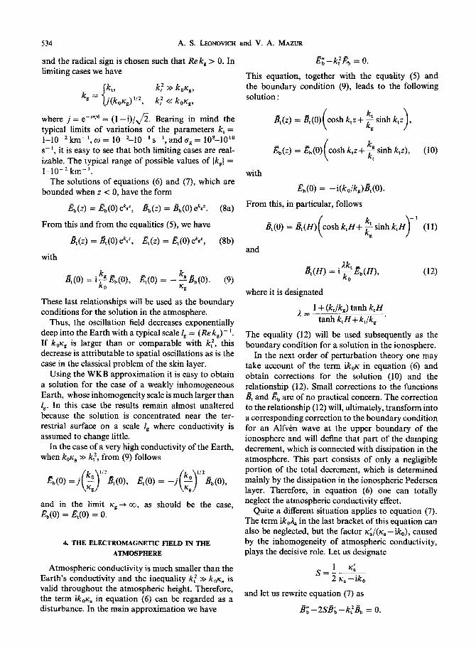
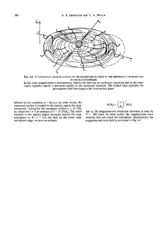
FIG. Al. A CONCEPTUAL REPRESENTATION OF THE MAGNETOSONIC FIELD IN THE MERIDIONAL CROSS-SECTION OF THE MAGNETOSPHERE.
In the outer magnetosphere (transparency region) the field has an oscillatory character and in the inner region (opacity region) it decreases rapidly in the earthward direction. The dashed lines represent the
geomagnetic field lines lying in the cross-section plane.
defined by the condition w = R,(r,). In other words, the resonance surface is located in the opacity region for mag- R(R,) - + R(f),
netosound. Taking for the resonance surface r0 = (3-7)R, C-1’ E
we obtain for I= 3 an estimate off = (5-10)RE. The radial that is, the magnetosound amplitude decreases at least by function in the opacity region decreases inward the mag- S3 - 100 times. In other words, the magnetosonic wave netosphere as R - I-'. For the field on the lower mag- virtually does not reach the ionosphere. Qualitatively, the netospheric edge, we have an estimate magnetosound wave field is portrayed in Fig. Al.

![UvA-DARE (Digital Academic Repository) Modelling the ... · [6,10], triggering inflammatory mechanisms like platelets aggre-gation and formation, smooth muscle cells (SMCs) migration](https://img.pdfslide.net/doc/110x75/60a0a5756a20b8137b0adf9a/uva-dare-digital-academic-repository-modelling-the-610-triggering-inflammatory.jpg)