Embed Size (px)
Citation preview
To be submitted to International Journal for Numerical Methods in Engineering
1
An Embedded Statistical Method for Coupling Molecular Dynamics and Finite Element Analyses
E. Saether1∗, V. Yamakov2, and E.H. Glaessgen1
1NASA Langley Research Center, Hampton, VA 23681, USA 2National Institute of Aerospace, Hampton, VA 23666, USA
SUMMARY
The coupling of molecular dynamics (MD) simulations with finite element methods
(FEM) yields computationally efficient models that link fundamental material processes
at the atomistic level with continuum field responses at higher length scales. The
theoretical challenge involves developing a seamless connection along an interface
between two inherently different simulation frameworks. Various specialized methods
have been developed to solve particular classes of problems. Many of these methods link
the kinematics of individual MD atoms with FEM nodes at their common interface,
necessarily requiring that the finite element mesh be refined to atomic resolution. Some
of these coupling approaches also require simulations to be carried out at 0 K and restrict
modeling to two-dimensional material domains due to difficulties in simulating full three-
dimensional material processes. In the present work, a new approach to MD-FEM
coupling is developed based on a restatement of the standard boundary value problem
used to define a coupled domain. The method replaces a direct linkage of individual MD
atoms and finite element (FE) nodes with a statistical averaging of atomistic
displacements in local atomic volumes associated with each FE node in an interface
region. The FEM and MD computational systems are effectively independent and
communicate only through an iterative update of their boundary conditions. With the use
of statistical averages of the atomistic quantities to couple the two computational
schemes, the developed approach is referred to as an embedded statistical coupling
method (ESCM). ESCM provides an enhanced coupling methodology that is inherently
applicable to three-dimensional domains, avoids discretization of the continuum model to
atomic scale resolution, and permits finite temperature states to be applied.
∗ Corresponding author: Tel.: +757-864-8079; fax: +757-864-8911. E-mail address: [email protected] (E. Saether)
https://ntrs.nasa.gov/search.jsp?R=20090024836 2018-12-27T17:30:17+00:00Z
To be submitted to International Journal for Numerical Methods in Engineering
2
1. INTRODUCTION
The emerging field of nanomechanics is providing a new focus in the study of the
mechanics of materials, particularly that of simulating fundamental atomic mechanisms
involved in the initiation and evolution of damage. These simulations are commonly
based on either quantum mechanics (ab-initio, tight-binding (TB) or density-functional
theory (DFT)) methods, on classical molecular dynamics (MD), or molecular statics
(MS) methods. These predictions of material behavior at nanometer length scales promise
the development of physics-based 'bottom-up' multiscale analyses that can aid in
understanding the evolution of failure mechanisms across length scales. However,
modeling atomistic processes quickly becomes computationally intractable as the system
size increases. With current computer technology, the computational demands of
modeling suitable domain sizes (on the order of hundreds of atoms for quantum
mechanics-based methods, and potentially billions of atoms for classical mechanics-
based methods) and integrating the governing equations of state over sufficiently long
time intervals, quickly reaches an upper bound for practical analyses. In contrast,
continuum mechanics methods such as the finite element method (FEM) provide an
economical numerical representation of material behavior at length scales in which
continuum assumptions apply. However, all constitutive relationships, kinematics, etc,
must be assumed a priori.
The concept of bridging length scales by concurrently coupling atomistic and
continuum computational paradigms is particularly attractive as a highly efficient means
of reducing the computational cost of simulations in cases that require modeling of
relatively large material domains to capture the complete deformation field, but where
atomic and subatomic refinement is needed only in very localized regions. Such
computational issues arise in modeling crack nucleation and propagation, and in
modeling dislocation formation and interaction. By using coupled models, the size
limitations of the atomistic simulation can be minimized by embedding an inner region
where complex dynamic processes and large deformation gradients exist within an outer
domain where the deformation gradients are small so that a continuum finite element
method (FEM) representation of the material becomes appropriate.
To be submitted to International Journal for Numerical Methods in Engineering
3
Over the past decade, various methods have been developed to address different
problems involving atomistically large material domains [1-12]. The most challenging
problem in developing these coupled methods is the formulation of a seamless
computational connection along an interface between different material representations.
A brief review of several representative coupling procedures follows to illustrate the
current state-of-the-art.
In coupling atomistic and continuum material representations, the continuity of
material properties must be maintained while transitioning from individual atoms
interacting through nonlocal forces to the local stress-strain field formalism of continuum
mechanics. For crack problems, the early efforts of Gumbsch and Beltz [10] led to the
development of the Finite Element – Atomistic (FEAt) coupling procedure that combined
an embedded MD system with a finite element domain. A generalized formulation of
conventional FEM, which allows FEM nodes to be considered as coarse-grained MD
“atoms” led to another computational scheme for atomistic-continuum coupling called
Coarse Grained Molecular Dynamics (CGMD). A detailed discussion of CGMD is given
by Rudd and Broughton [11,12]. In yet another coupling method, the Coupling of Length
Scales (CLS) method [2], the nodes in a finite element model representing the continuum
region are directly connected to the atoms in an atomistic region forming an interface of
“pad” atoms. The region of “pad” atoms, used in this and other atomistic-continuum
coupling methods, serves to minimize surface tension effects on the atoms in the
atomistic system but also introduces a constraint due to the elasticity of the interface
region. The constraining effect of this region is generally considered insignificant and is
ignored.
The Quasicontinuum (QC) method, reviewed by Miller and Tadmor [6], is formally
based on an entirely atomistic description of the material domain. However, for
computational efficiency, regions are identified in which discrete atoms may be grouped
to form a local continuum. The particular representation used is determined by evaluating
the magnitude of local deformation gradients and dictates the treatment of
“representative atoms” or “repatoms.” In the QC formalism, “non-local repatoms” are
used to represent “real” atoms to form atomistic regions treated by MS/MD methods
while “local repatoms” are used to define continuum domains by applying both the
To be submitted to International Journal for Numerical Methods in Engineering
4
Cauchy-Born rule [13] and aspects of FEM. The interaction of local and nonlocal
repatoms at the atomistic/continuum interface leads to the generation of “ghost forces”
that must be mitigated through the introduction of “dead loads” that are iterated for self-
consistency in the force balance at the interface between subregions.
Another representative coupling approach is the bridging method of Xiao and
Belytschko [7] and is based on an overlay approach in which MD and FEM
representations are superposed in an interface region. This method allows interpolated
FEM nodal displacements to be associated with atomic displacements in the bridging
domain.
The Coupled Atomistic/Dislocation Dynamics (CADD) method of Shilkrot et al. [8]
is specifically designed to simulate, identify and pass dislocations between atomistic and
continuum domains. The method was originally limited to 0 K simulations [8]; but has
been recently extended to include finite temperature effects in the MD system by linking
the MD to a quasistatic FEM domain through a thermal damping region [9]. Currently,
CADD uses a two-dimensional material representation due to the complexity of passing
fully three-dimensional dislocations between the MD and FEM domains.
A common feature of many of these approaches [1-12] for coupling atomistic and
continuum representations is the refinement of the finite element (FE) mesh to atomic
length scales to link the kinematics of the FE nodes to that of the discrete atoms along an
interface. In this paper, approaches that relate atoms and FE nodes in a one-to-one
manner, or through a form of interpolation, will be referred to as direct coupling (DC)
approaches.
While DC approaches are straightforward, the fundamental difficulty in their
development lies in the inherent differences between the atomistic and continuum
computational models. The physical state of the atomistic region is described through
nonlocal interatomic forces between discrete atoms of given position and momentum,
while the physical state of the continuum region is described through continuous stress-
strain fields that reflect local statistical averages of atomic interactions at larger length
and time scales. In general, the formal connection between continuum and discrete
quantities can only be achieved through an adequate statistical averaging over scales
where the discreteness of the atomic structure can be approximated as a continuum. A
To be submitted to International Journal for Numerical Methods in Engineering
5
consequence of some DC interfacing strategies in their initial formulation, such as QC,
required that the analysis be performed quasistatically at 0 K. Further details of the direct
coupling methods may be found in the original publications and in several general review
papers [4-6].
In this paper, an alternative approach to the DC approaches is proposed to construct
a coupled MD-FEM system. The approach is based on solving a coupled boundary value
problem (BVP) at the MD/FE interface for a MD region embedded within a FEM
domain. The method uses statistical averaging over both time and volume in atomistic
subdomains at the MD/FE interface to determine nodal displacement boundary conditions
for the continuum FE model. These enforced displacements, in turn, generate interface
reaction forces that are applied as constant traction boundary conditions [14-16] between
updates of the FEM solution to the atoms within the localized MD subdomains. Thus, the
present approach may be described as a local-nonlocal BVP because it relates local
continuum nodal quantities with nonlocal statistical averages of atomistic quantities over
selected atomic subdomains. An iterative procedure between the MD statistical
displacements and the FEM reaction forces ensures continuity at the interface. In this
way, the problem of redefining continuum variables at the atomic scale is avoided, and
the developed interface approach links different time and length scales between the MD
region and FEM domain.
With the emphasis of using statistical averages to couple the two computational
schemes, the developed approach is identified as a statistical coupling (SC) approach.
Based on the SC approach, the developed MD-FEM coupling method is referred to as the
embedded statistical coupling method (ESCM). ESCM provides an enhanced coupling
methodology that is inherently applicable to three-dimensional domains, avoids
discretization of the continuum model to atomic scale resolution, permits arbitrary
temperatures to be applied, and treats, in a rigorous manner, the compensation of surface
effects in the MD system.
This paper will detail the ESCM approach for coupling MD and FEM computational
domains for the case of systems that reach thermodynamic equilibrium or evolve
quasistatically. While there is no principle difficulty in implementing this approach for
To be submitted to International Journal for Numerical Methods in Engineering
6
non-equilibrium systems, it is beneficial to first consider the case of equilibrium
simulations to illustrate initial applications of this methodology.
The remainder of this paper is organized as follows. Section 2 describes the structure
of the coupled MD-FEM model. This includes discussions of the MD and FEM material
representations, the coupling interface, and the iterative MD-FEM coupling methodology.
Section 3 presents several validation studies to substantiate the accuracy of the developed
methodology. Section 4 presents concluding remarks on the overall effectiveness of the
ESCM. Details of internal force calculations involved in the coupling procedure and a
discussion of model generation are contained in separate appendices.
2. THE ESCM MODEL
The ESCM approach is developed to reduce computational costs incurred while
simulating “large” volumes of material by embedding an inner atomistic MD system
within a surrounding continuum FEM domain. In principal, the shape of the atomistic
region may be arbitrary as shown in Figure 1; however, for simplicity, the special case of
a circular region is utilized in the present work. Similarly, although any constitutive
behavior may be assumed for the FEM domain, the present study considers a linear
elastic continuum.
The structure of the ESCM model consists of four regions: 1) an Inner MD Region; 2)
an Interface MD Region wherein MD and finite elements are superimposed; 3) a Surface
MD Region that does not interact with the FE nodes but is used to compensate for atomic
free edge effects; and 4) a FEM domain in which standard finite element equations apply.
These four regions are depicted in Figure 2.
Complete details of the ESCM procedure will be presented by discussing general
aspects of the MD and FEM computational systems, followed by specific details of the
MD/FE Interface, the Surface MD Region and the MD-FEM coupling procedure.
2.1 MD and FEM model components
To be submitted to International Journal for Numerical Methods in Engineering
7
The Inner MD Region is used to model material phenomena at the atomistic level.
This Inner MD Region should be large enough to ensure a statistically smooth transition
from a continuum to an atomistic representation while modeling any of the types of
processes (e.g., dislocation formation, void nucleation, or crack propagation) that are
required by the simulation. Together, the Inner, Interface, and Surface MD Regions
constitute the complete MD system.
It is important to emphasize that the partitioning of the MD system into different
regions is not a physical separation of the system. An atom assigned to a particular
location freely interacts with atoms in its interaction neighborhood that may reside in a
different region. Thus, the overall simulation is performed using any conventional MD
technique without any imposition of direct kinematic constraints. The only difference
between the three MD regions is that, while the atoms in the Inner MD Region are
subject only to their interatomic forces, the Interface and Surface MD Regions serve the
added purpose of facilitating the application of external forces involved in the ESCM
procedure.
The addition of a FEM domain permits a large reduction in the computational cost of
simulations by replacing the atomistic representation with a continuum model in those
parts of the system where the deformation gradients are small and atomic-level resolution
is not necessary. The current application uses the FEM domain to simulate an extended
material model such that the elastic deformation and load transfer due to applied far-field
boundary conditions are accurately transferred to the Inner MD Region. The continuum
field is currently assumed to be static with linear elastic material properties but other
applications of ESCM might require the incorporation of nonlinear material behavior,
such as plasticity or general dynamic response, where nonlinear processes generated in
the Inner MD Region can be propagated into the continuum.
2.2 MD/FE interface
The main role of the MD/FE Interface is to provide a computational linkage between
the MD region and FEM domain. The atoms that surround a given FE node at the
To be submitted to International Journal for Numerical Methods in Engineering
8
interface are partitioned to form a cell in the Interface MD Region, called an interface
volume cell (IVC), as shown in Figure 2. A similar partitioning is also applied to the
Surface MD Region, forming surface volume cells (SVCs). The IVCs compute averaged
MD displacements at their mass center that are then prescribed as displacement boundary
conditions to the associated interface finite element nodes. The IVCs need not coincide in
size or shape with the finite element to which the FE node belongs. In the model
described in this paper, the IVCs are formed through a Voronoi-type construction [17] by
selecting those atoms with a common closest finite element node.
Typically, one finite element at the interface encompasses a region of several hundred
to several thousand atoms. A lower bound for the number of atoms associated with each
finite element node is determined by the requirement of obtaining a minimally fluctuating
average of atomic displacements and minimizing the magnitude of generated gradients in
the MD region bordering the FEM domain. With an effective average at this scale, the
discreteness of the atomic structure is homogenized enough so that the FEM domain
responds to the atomistic region as an extension of the continuum.
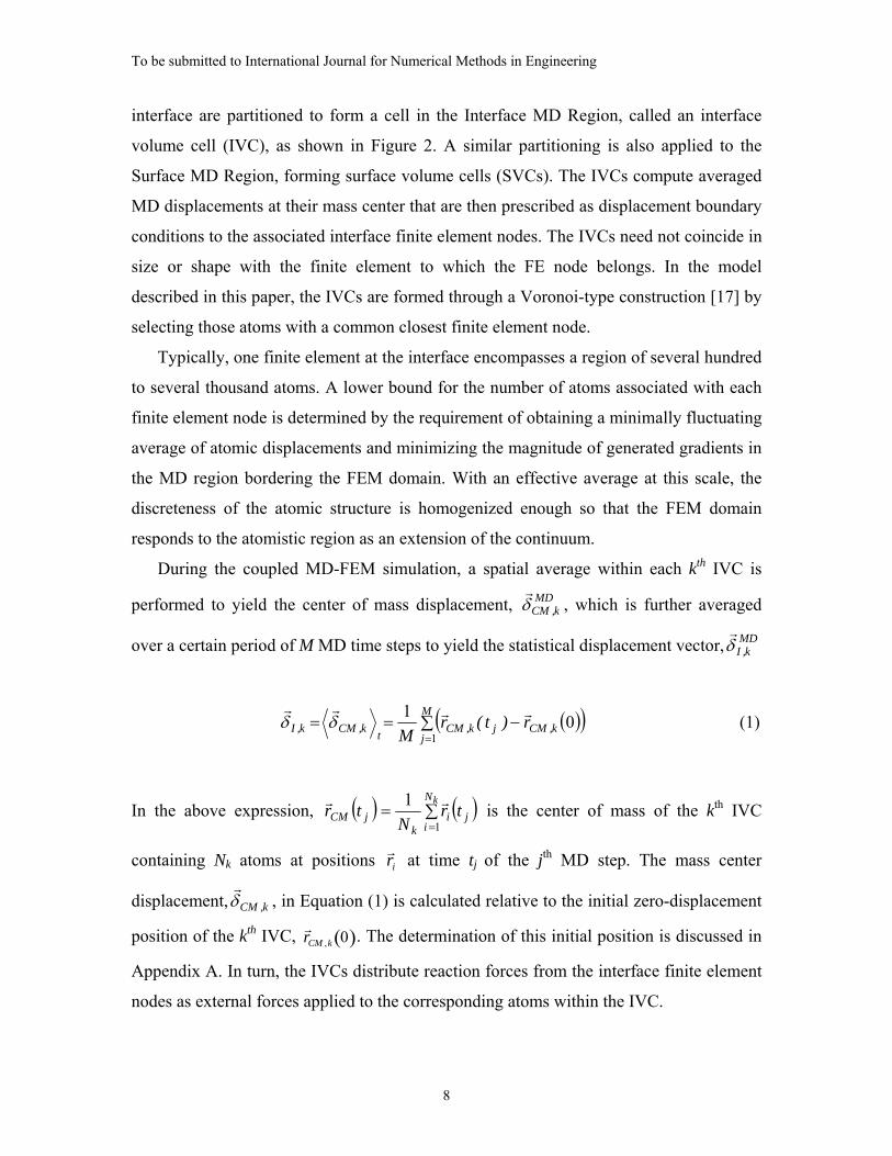
During the coupled MD-FEM simulation, a spatial average within each kth IVC is
performed to yield the center of mass displacement, MDk,CMδ
r, which is further averaged
over a certain period of M MD time steps to yield the statistical displacement vector, MDk,Iδ
r
( )( )∑ −===
M
jk,CMjk,CMtk,CMk,I r)t(r
M 101 rrrr
δδ (1)
In the above expression, ( ) ( )∑==
kN
iji
kjCM tr
Ntr
1
1 rr is the center of mass of the kth IVC
containing Nk atoms at positions irr at time tj of the jth MD step. The mass center
displacement, k,CMδr
, in Equation (1) is calculated relative to the initial zero-displacement
position of the kth IVC, r r CM ,k 0( ). The determination of this initial position is discussed in
Appendix A. In turn, the IVCs distribute reaction forces from the interface finite element
nodes as external forces applied to the corresponding atoms within the IVC.
To be submitted to International Journal for Numerical Methods in Engineering
9
2.3 Surface MD Region
In order for the MD domain to deform freely in response to applied reaction forces, it
is modeled using free surface boundary conditions as discussed in [13,14]. However, the
existence of a free surface introduces several undesirable effects in the MD system. First,
it creates surface tension forces that must be removed to avoid distorting the MD
response. Second, because atoms at or near the free surface do not have a complete set of
interacting neighboring atoms, the coordination number of the surface atoms is reduced
so they are less strongly bonded to the surrounding atomic field than those within the
interior. Under sufficiently large reaction forces, these atoms may be separated from the
surface layer causing a surface degradation within the MD domain. To mitigate these free
surface effects and to stabilize the atoms in the Interface MD Region, an additional
volume of outlying atoms constituting a Surface MD Region is introduced as shown in
Figure 2.
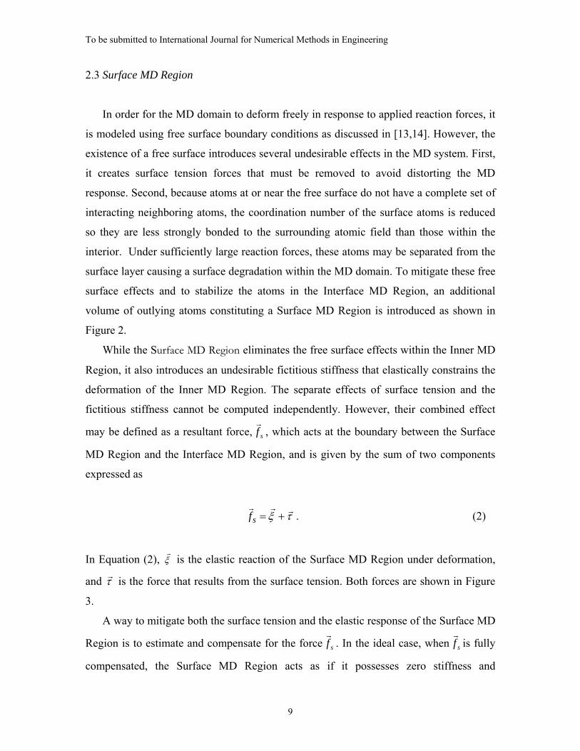
While the Surface MD Region eliminates the free surface effects within the Inner MD
Region, it also introduces an undesirable fictitious stiffness that elastically constrains the
deformation of the Inner MD Region. The separate effects of surface tension and the
fictitious stiffness cannot be computed independently. However, their combined effect
may be defined as a resultant force, sfr
, which acts at the boundary between the Surface
MD Region and the Interface MD Region, and is given by the sum of two components
expressed as
τξ rrr+=sf . (2)
In Equation (2), ξr
is the elastic reaction of the Surface MD Region under deformation,
and τr is the force that results from the surface tension. Both forces are shown in Figure
3.
A way to mitigate both the surface tension and the elastic response of the Surface MD
Region is to estimate and compensate for the force sfr
. In the ideal case, when sfr
is fully
compensated, the Surface MD Region acts as if it possesses zero stiffness and
To be submitted to International Journal for Numerical Methods in Engineering
10
experiences no surface tension, thereby mitigating spurious influences on the Inner MD
Region. Subdividing the Surface MD Region into a number of SVCs helps to follow the
variations of sfr
along the perimeter of the Interface MD Region. For convenience, the
partitioning of SVCs can be made to follow the IVC partitioning of the Interface MD
Region. The resultant force is then calculated individually for each SVC. To compensate
for sfr
, a counterforce, cfr
, is computed along the IVC/SVC interface and then distributed
over the atoms of each SVC in a similar manner as the nodal reaction forces are applied
to the IVCs of the Interface MD Region. The calculation of the counterforce, cfr
, is
presented in Appendix B.
2.4 Phonon Damping
Both the IVCs and SVCs serve the additional role of providing a dissipative damping
mechanism for phonons propagating into the interface. Potential sources of phonon
generation are the application of the FEM reaction forces to the IVCs and the resonant
elastic oscillations in the dynamic MD region. Phonons can also be generated from within
the Inner MD Region as a result of simulated atomistic processes. In the current
application of ESCM, these oscillations must be damped in order to achieve equilibrium
with the static FEM domain. A number of different damping schemes have been
addressed in the literature. Holian and Ravelo [18], and more recently, Schäfer et al. [19],
found that applying linearly increasing viscous damping to the atoms in a region
surrounding the center of the MD system can effectively absorb the intense phonon
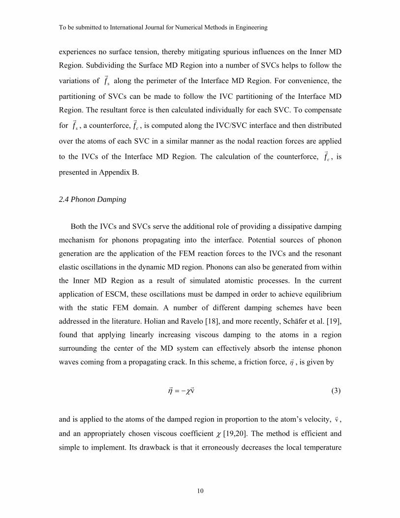
waves coming from a propagating crack. In this scheme, a friction force, ηr , is given by
vrr
χη −= (3)
and is applied to the atoms of the damped region in proportion to the atom’s velocity, vr ,
and an appropriately chosen viscous coefficient χ [19,20]. The method is efficient and
simple to implement. Its drawback is that it erroneously decreases the local temperature
To be submitted to International Journal for Numerical Methods in Engineering
11
in the damping region resulting in undesirable strain gradients because of thermal
contraction.
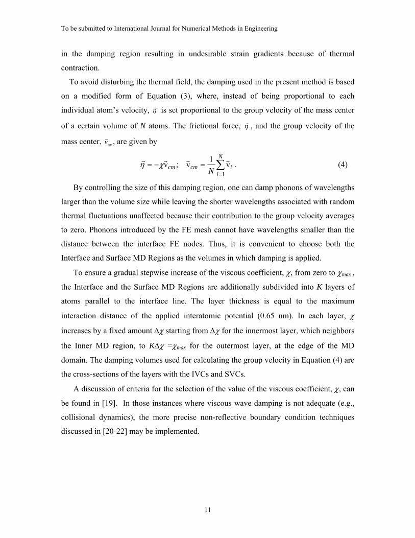
To avoid disturbing the thermal field, the damping used in the present method is based
on a modified form of Equation (3), where, instead of being proportional to each
individual atom’s velocity, ηr is set proportional to the group velocity of the mass center
of a certain volume of N atoms. The frictional force, ηr , and the group velocity of the
mass center, cmvv , are given by
∑=
=−=N
iicmcm N
;1
v1vv rrrrχη . (4)
By controlling the size of this damping region, one can damp phonons of wavelengths
larger than the volume size while leaving the shorter wavelengths associated with random
thermal fluctuations unaffected because their contribution to the group velocity averages
to zero. Phonons introduced by the FE mesh cannot have wavelengths smaller than the
distance between the interface FE nodes. Thus, it is convenient to choose both the
Interface and Surface MD Regions as the volumes in which damping is applied.
To ensure a gradual stepwise increase of the viscous coefficient, χ, from zero to χmax ,
the Interface and the Surface MD Regions are additionally subdivided into K layers of
atoms parallel to the interface line. The layer thickness is equal to the maximum
interaction distance of the applied interatomic potential (0.65 nm). In each layer, χ
increases by a fixed amount Δχ starting from Δχ for the innermost layer, which neighbors
the Inner MD region, to KΔχ =χmax for the outermost layer, at the edge of the MD
domain. The damping volumes used for calculating the group velocity in Equation (4) are
the cross-sections of the layers with the IVCs and SVCs.
A discussion of criteria for the selection of the value of the viscous coefficient, χ, can
be found in [19]. In those instances where viscous wave damping is not adequate (e.g.,
collisional dynamics), the more precise non-reflective boundary condition techniques
discussed in [20-22] may be implemented.
To be submitted to International Journal for Numerical Methods in Engineering
12
2.5 MD-FEM coupling
The MD-FEM coupling in the ESCM is achieved through an iterative equilibration
scheme between the MD region and the FEM domain. In this scheme, iterations begin
with displacements at the MD/FE Interface that are calculated as statistical averages over
the atomic positions within each IVC and averaged over the time of the MD analysis.
These average displacements are then imposed as displacement boundary conditions,
{ Iδv
}, on the FEM domain. The resulting FEM BVP is then solved to recover new
interface reaction forces, { IRv
}, resulting from the applied interface displacements and
any imposed far-field loading. The new interface reaction forces, { IRv
}, are then
distributed to the atoms in the IVCs, thus defining new constant traction boundary
conditions on the MD system. Between the FEM solution updates, the traction boundary
conditions are constant and applied to the MD region to ensure that the elastic field from
the FEM domain is correctly duplicated in the atomistic region. The MD-FEM iteration
cycle repeats until a stable equilibrium of both displacements and forces between the
atomistic and continuum material fields is established at the interface.
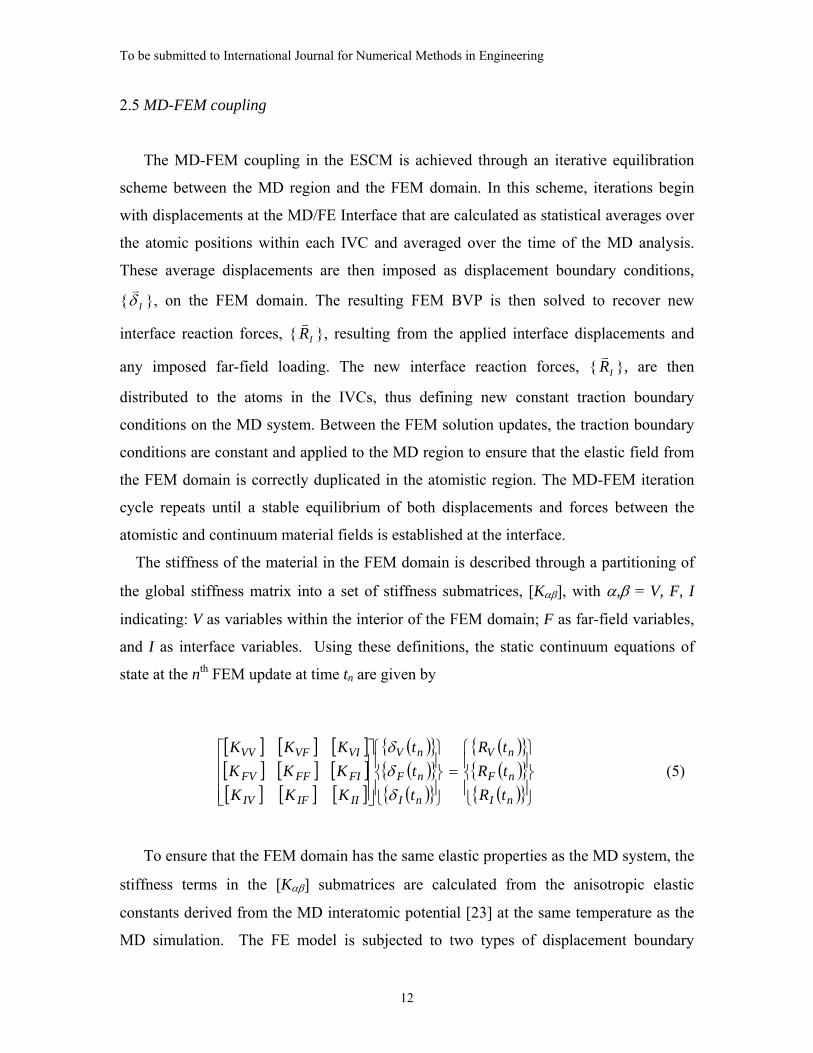
The stiffness of the material in the FEM domain is described through a partitioning of
the global stiffness matrix into a set of stiffness submatrices, [Kαβ], with α,β = V, F, I
indicating: V as variables within the interior of the FEM domain; F as far-field variables,
and I as interface variables. Using these definitions, the static continuum equations of
state at the nth FEM update at time tn are given by
[ ] [ ] [ ][ ] [ ] [ ][ ] [ ] [ ]
( ){ }( ){ }( ){ }
( ){ }( ){ }( ){ }⎪
⎭
⎪⎬
⎫
⎪⎩
⎪⎨
⎧=
⎪⎭
⎪⎬
⎫
⎪⎩
⎪⎨
⎧
⎥⎥⎥
⎦
⎤
⎢⎢⎢
⎣
⎡
nI
nF
nV
nI
nF
nV
IIIFIV
FIFFFV
VIVFVV
tRtRtR
ttt
KKKKKKKKK
δδδ
(5)
To ensure that the FEM domain has the same elastic properties as the MD system, the
stiffness terms in the [Kαβ] submatrices are calculated from the anisotropic elastic
constants derived from the MD interatomic potential [23] at the same temperature as the
MD simulation. The FE model is subjected to two types of displacement boundary
To be submitted to International Journal for Numerical Methods in Engineering
13
conditions: (1) the far-field displacements {δF}, which define the load over the entire
coupled MD-FEM system; and (2), the interface displacements { } ( )kIIII ,.,.., δδδδ
vvv 21= ,
which represent the deformation response of the MD system at the 1st, 2nd, ... , and kth
IVC.
The solution for the unknown displacements in the interior of the FEM domain, { }Vδ ,
is given by
δV tn( ){ } = KVV[ ] −1 RV tn( ){ }− KVF[ ] δF tn( ){ }− KVI[ ] δ I tn( ){ }( ) (6)
which allows the calculation of the interface reaction forces, ( ){ } ,..),..,( 21 kIIInI RRRtR
vvv=
of the 1st, 2nd, ... , and kth IVC to be obtained from
RI tn( ){ }= KIV[ ] δV tn( ){ }+ KIF[ ] δF tn( ){ }+ KII[ ] δ I tn( ){ } (7a)
together with the far-field forces of constraint
RF tn( ){ } = KFV[ ] δV tn( ){ }+ KFF[ ] δF tn( ){ }+ KFI[ ] δ I tn( ){ } (7b)
The dynamics of an atom i of mass m(i) at position r(i) in the embedded MD regions is
described by Newton’s equations of motion
( )( ) egionRMDSurfaceSVCi;Nffrm
RegionMDInterfaceIVCi;NRfrmRegionMDInneri;frm
kkcm
kS
kciii
kkcm
kI
kIiii
iii
∈−+=∈−+=∈=
vvvvv
&&v
vvv&&v
v&&v
χχ (8)
The atoms in the Inner MD Region experience only the atomic force ( )∑=j
jii ff ,
vv
resulting from their jth neighbors. The term ( )jif ,v
is expressed by Equation (B4) as shown
in Appendix B. The atoms in the interface region, assigned to a given kth IVC, are
subjected to the additional external force, kIR
v (Equation (7a)), which is distributed over
To be submitted to International Journal for Numerical Methods in Engineering
14
the number of contained atoms, N Ik . The atoms in the Surface MD Region belonging to a
given kth SVC experience the additional counterforce, kcf
v, which is distributed over the
N Sk atoms contained in their volume. In order to maintain the continuity of forces
between adjacent cells, the force distribution is interpolated with a linear (or higher order)
interpolation between atomic positions as a function of each atom’s distance from the
mass center of its associated cell. In the present study, a simple linear interpolation was
applied. For the equations governing the Interface and the Surface MD Regions in
Equation (8), the viscous friction force, kcmvvχ , defined in Equation (4), is applied
uniformly to the atoms contained within the IVCs and SVCs.
During the MD integration of Equation (8) for a period ΔtM = MΔt, where M is the
number of time steps and Δt is the duration of the time step, the new average
displacements ( ){ }1+nI tδ are computed from Equation (1). The new atomistic
displacements for the next FEM update at time tn+1 = tn + ΔtM are reapplied in Equations
(6) and (7a) to calculate the next iterative update of the recovered forces, RI tn+1( ){ }.
During the same time interval, the compensation forces ( ){ }tfc are also evolving through
Equation (B15) (in Appendix B). The period ΔtM is selected by a determination of the
convergence rate to a state of dynamic equilibrium between the MD region and the FE
domain. Applying a suitable damping force (Equation 4) at the MD side of the interface
ensures a faster convergence rate. The algorithm for the entire coupled simulation is
summarized in Figure 4.
Indication for convergence between the MD and FEM domains is the convergence of
the interface forces {RI} and displacements {δ I} to equilibrium steady-state values. This
convergence can be achieved only if the MD system can reach a dynamic force balance
with the surrounding FEM system. A convergence criteria will be derived based on the
force balance between the atomic forces in the MD system and the reaction forces in the
FEM domain. At equilibrium, the averaged in time motion of the IVC mass centers is
zero, or
0==t
kCMt
vr kCM
v&v , (9a)
To be submitted to International Journal for Numerical Methods in Engineering
15
and the change of the averaged total momentum, Δpk t , of any kth IVC due to the FEM
reaction force for the period of the MD simulation of M time steps is also zero, or
( ) 0ttrmpM
1n
N
1iniik
kI
=∑ ∑ Δ=Δ= =
&&vv . (9b)
Performing the same double summation on the second equation in Equation (8)
results in
( ) kI
t
N
ii
M
m
N
imi Rftf
M
kI
kI vvv
−== ∑∑∑== = 11 1
1 (10)
which states that, at equilibrium and in accordance with Newton’s 3rd law, the FEM
reaction force becomes equal and opposite to the average MD atomic force in the
corresponding kth IVC. Equation (10) thus expresses the establishment of static force
equilibrium between the MD system and the FEM domain and can be used as a
convergence criteria for the iterative MD-FEM coupling procedure.
A discussion of practical issues regarding model generation for applying the ESCM
procedure is presented in Appendix A.
3. NUMERICAL VERFICATION OF THE ESCM
3.1 The simulation models
Four test cases are considered to investigate the behavior of ESCM. First, the
effectiveness of the application of compensation forces for the mitigation of surface
tension effects is examined. Second, the dynamic behavior of the MD system is explored
by varying the rate and sequence of applied external loads. Third, the stress-strain
continuity between the MD region and the FEM domain is assessed through comparison
with an exact solution of an elastically deformed plate with a circular hole. Fourth, a
simulation of the propagation of an edge crack through the FEM domain into the MD
system is performed to determine the suitability of ESCM for solving problems related to
crack growth.
To be submitted to International Journal for Numerical Methods in Engineering
16
The model geometry used in all of the verification studies is shown in Figure 5. This
model consists of a circular Inner MD Region of diameter, dMD, that is embedded in a
larger exterior square FEM domain of elastic material with a side dimension of dFE =
20dMD. A general discussion of issues related to model construction in applying ESCM is
presented in Appendix A, while the specifics of the MD and FE models will be discussed
next.
3.1.1 The MD model
The material for the simulation models was chosen to be a perfect crystal of
aluminum. The atomic properties of aluminum were represented by the embedded atom
model (EAM) potential of Mishin et al. [24], which was fitted to give the correct zero-
temperature lattice constant, ao = 0.405 nm, elastic constants, cohesive energy, vacancy
formation energy, etc. For accurate coupling, material properties of the FE model are
obtained directly from the EAM interatomic potential.
The first three test simulations, presented in Sections 3.2.1 to 3.2.3, use a common
MD system which will be described here. The forth test is performed on a bicrystal MD
model which will be described in Section 3.2.4. For the first three tests, the MD domain
is constructed as a circular disk of monocrystalline aluminum with its main
crystallographic axes [1 0 0], [0 1 0], and [0 0 1] oriented along the x-, y- and z-
directions, respectively. The MD system is simulated with periodic boundary conditions
along the z-direction and with free surface boundary conditions along its perimeter. These
boundary conditions allow the MD domain to deform in an unconstrained manner in the
x-y plane under the external reaction forces from the FEM domain while maintaining
constant zero pressure along the z-direction using the Parrinello-Rahman constant-
pressure simulation technique [25]. Constant temperature is maintained by applying the
Nose-Hoover thermostat [26] in the Inner MD Region only. The thickness of the plate
along the z-axis is equal to h = 5ao ≈ 2.0 nm (Figure 5). Though very thin, the MD system
mechanically behaves as an infinitely thick plate due to the applied periodic boundary
conditions along the z- direction. The test simulations were performed at near zero
temperature (T = 10 K) to minimize the thermal noise, and at room temperature (T = 300
To be submitted to International Journal for Numerical Methods in Engineering
17
K) to demonstrate ESCM for more practically relevant situations in which thermal effects
are important. For the models used in the present work, effective viscous wave damping
in the Interface and the Surface MD Regions was achieved by setting χmax = 3 eVps/nm2.
For this χ and a damping layer with a width of 0.65 nm, the effective average temperature
in the damping volumes decreased by only 10% compared to the bulk temperature.
Four different models were prepared with the diameter of the circular MD system
varying from 22 nm to 164 nm. Reference positions of the IVC mass centers, ( )0rCMr ,
were determined using methods outlined in Appendix A. The width of the Surface MD
Region, defined at the free surface of the MD system, was fixed at 2 nm.
3.1.2 The FE model
The elastic continuum region was modeled using 8-node hybrid-stress hexahedral
finite elements that have a reduced sensitivity to mesh distortion compared to standard
displacement-based elements, and allow explicit stiffness coefficients to be analytically
derived, thereby minimizing their computational requirements [27,28]. The elastic
constants in the material constitutive matrix were derived from the interatomic potential
for pure aluminum at T = 10 K. The values were averaged for uniaxial stresses from 100
to 500 MPa, accounting for the non-linear material properties, as: C11 = 112.7 GPa, C12 =
59.4 Gpa, and C44 = 30.6 GPa. These values differ by only 3% from the static, zero
Kelvin elastic constants reported for this potential in [24].
The continuum finite element model contains an open inner region of diameter dMD,
within which the atomistic domain is embedded. Along its perimeter, 80 nodes at z =
+h/2 and 80 nodes at z = -h/2 were placed to form 160 FE interface nodes to
communicate with the embedded MD system.
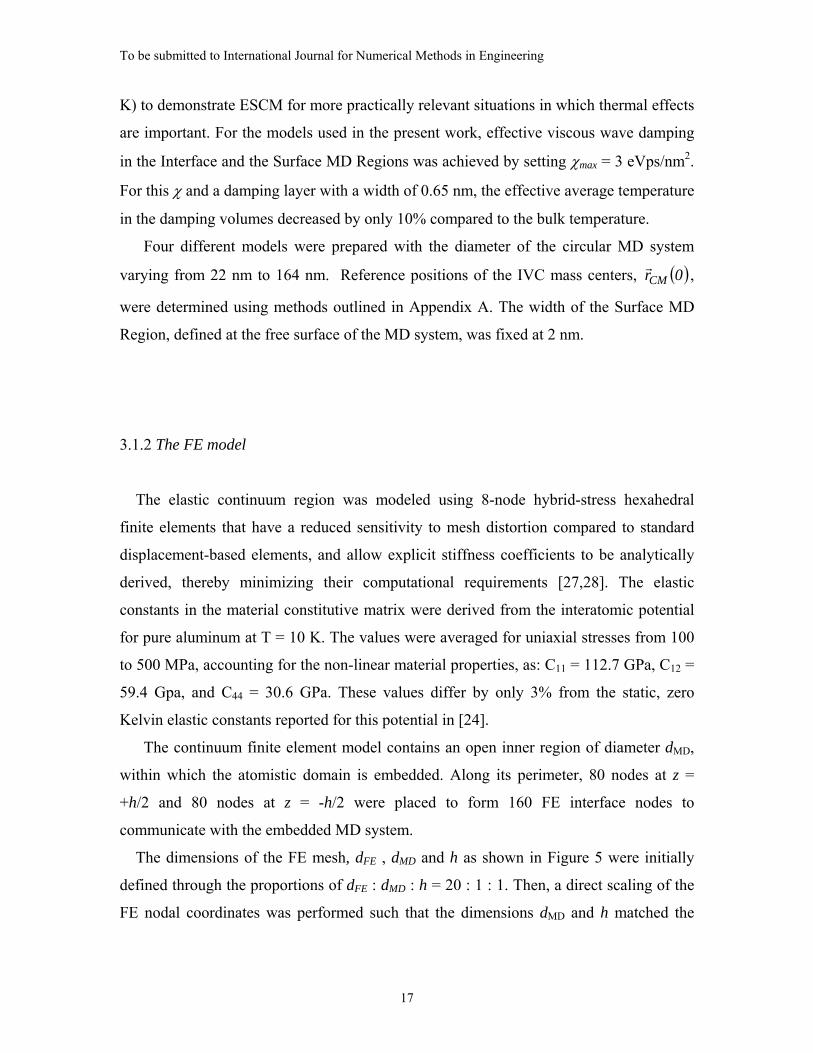
The dimensions of the FE mesh, dFE , dMD and h as shown in Figure 5 were initially
defined through the proportions of dFE : dMD : h = 20 : 1 : 1. Then, a direct scaling of the
FE nodal coordinates was performed such that the dimensions dMD and h matched the
To be submitted to International Journal for Numerical Methods in Engineering
18
dimensions of the MD system. Finally, a second scaling of the FEM system was
performed to preserve the outer dimension ratio dFE : dMD = 20 : 1.
3.2 Numerical test results and analyses
The four test cases selected to interrogate the essential features of the ESCM are
presented in the following sections. Discussions assessing results and details of the
analyses are included to thoroughly investigate the verification simulations.
3.2.1 Verification of the surface tension and the Surface MD Region stiffness
compensation
The purpose of this simulation is to estimate the magnitude of the surface forces, their
effect on coupling the two computational domains, and the ability of the compensation
procedure to mitigate both surface tension effects and the spurious constraint of the
Surface MD Region stiffness. The simulation is performed for the case of a homogeneous
perfect crystal of aluminum. Because the effect of the surface tension is expected to be
relatively weak, the temperature of the simulations was kept at T = 10 K to minimize the
thermal noise and to increase the sensitivity of the force and pressure calculations.
The pressure inside the system due to surface tension is defined as the radial
component of the stress tensor, ps = σrr , averaged over an isolated MD system with free
surface boundary conditions in the x- and y-directions, and periodic, zero pressure
boundary conditions applied in the z-direction. The virial definition of stress [29] inside
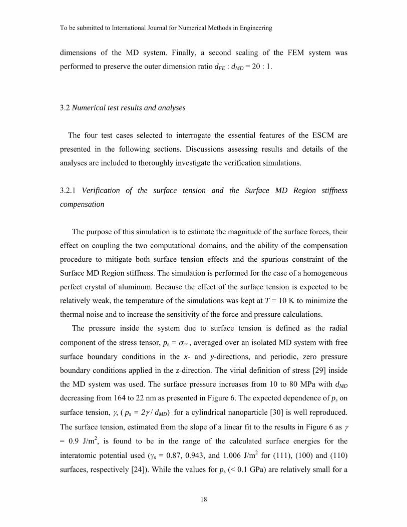
the MD system was used. The surface pressure increases from 10 to 80 MPa with dMD
decreasing from 164 to 22 nm as presented in Figure 6. The expected dependence of ps on
surface tension, γ, ( ps = 2γ / dMD) for a cylindrical nanoparticle [30] is well reproduced.
The surface tension, estimated from the slope of a linear fit to the results in Figure 6 as γ
= 0.9 J/m2, is found to be in the range of the calculated surface energies for the
interatomic potential used (γs = 0.87, 0.943, and 1.006 J/m2 for (111), (100) and (110)
surfaces, respectively [24]). While the values for ps (< 0.1 GPa) are relatively small for a
To be submitted to International Journal for Numerical Methods in Engineering
19
MD simulation (where typical loads are of the order of 1 GPa), particularly for small MD
systems, its contribution should not be neglected.
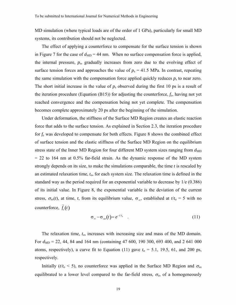
The effect of applying a counterforce to compensate for the surface tension is shown
in Figure 7 for the case of dMD = 44 nm. When no surface compensation force is applied,
the internal pressure, ps, gradually increases from zero due to the evolving effect of
surface tension forces and approaches the value of ps = 41.5 MPa. In contrast, repeating
the same simulation with the compensation force applied quickly reduces ps to near zero.
The short initial increase in the value of ps observed during the first 10 ps is a result of
the iteration procedure (Equation (B15)) for adjusting the counterforce, fc, having not yet
reached convergence and the compensation being not yet complete. The compensation
becomes complete approximately 20 ps after the beginning of the simulation.
Under deformation, the stiffness of the Surface MD Region creates an elastic reaction
force that adds to the surface tension. As explained in Section 2.3, the iteration procedure
for fc was developed to compensate for both effects. Figure 8 shows the combined effect
of surface tension and the elastic stiffness of the Surface MD Region on the equilibrium
stress state of the Inner MD Region for four different MD system sizes ranging from dMD
= 22 to 164 nm at 0.5% far-field strain. As the dynamic response of the MD system
strongly depends on its size, to make the simulations comparable, the time t is rescaled by
an estimated relaxation time, to, for each system size. The relaxation time is defined in the
standard way as the period required for an exponential variable to decrease by 1/e (0.386)
of its initial value. In Figure 8, the exponential variable is the deviation of the current
stress, σxx(t), at time, t, from its equilibrium value, σ∞, established at t/to = 5 with no
counterforce, r f c t( )
σ∞ − σ xx t( )= e− t /to . (11)
The relaxation time, to, increases with increasing size and mass of the MD domain.
For dMD = 22, 44, 84 and 164 nm (containing 47 600, 190 300, 693 400, and 2 641 000
atoms, respectively), a curve fit to Equation (11) gave to = 5.1, 19.5, 61, and 200 ps,
respectively.
Initially (t/to < 5), no counterforce was applied in the Surface MD Region and σxx
equilibrated to a lower level compared to the far-field stress, σo, of a homogeneously
To be submitted to International Journal for Numerical Methods in Engineering
20
strained plate. The stress due to the Poisson contraction of the unconstrained boundaries
( y = ± dFE 2), σyy, also deviated from the expected zero level. The reason for these
deviations is the combined effect of surface tension and the elastic stiffness of the Surface
MD Region. The deviations of both σxx and σyy decrease proportionally to the increase of
dMD, as expected because of the decreasing surface-to-volume ratio. When the
counterforce is applied (t/to > 5), the effect of the spurious forces in the Surface MD
Region for all of the tested MD systems of dMD from 22 to 164 nm is almost entirely
negated.
3.2.2 Simulation of the dynamics of the coupled MD-FEM system
The dynamic behavior of the coupled MD-FEM system in the simplest case of a
uniformly loaded homogeneous aluminum plate is depicted in Figure 9. The figure
presents the stress response of the Inner MD Region to the applied far-field strain. The
system is the same as that used for the results in Figure 7, with dMD = 44 nm. In this
numerical test, the prescribed strain of εxx = 0.5% was reached in two ways: first, by an
instantaneously applied far-field strain of 0.5% at the outer-boundaries of the FEM
domain, and second, by five consecutive increments of 0.1% each. In both cases, the
length of the MD iteration simulation was ΔtM = MΔt = 1 ps with M = 500 and Δt = 2 fs.
The tensile component of the stress in the MD system, σxx, converges to nearly the
same value for both cases shown in Figure 9 and is very close to the far-field stress of the
FEM domain, σo (σxx → 354 MPa and σo = 358.5 MPa). Similarly, σyy quickly relaxes to
zero after a temporary jump in response corresponding to each increase in the applied far-
field strain. The test shows that the state of equilibrium, wherein the MD system is in
force balance with the FEM domain, is obtained with little dependence on step size for
monotonic loading up to 0.5% strain.
After each strain increment of 0.1%, the MD system reached equilibrium with the
FEM domain within approximately 25 ps, which is consistent with the estimate for to =
19.5 ps in Figure 7 for dMD = 44 nm. This time was approximately the same as for the
instantaneous jump to 0.5%. The relatively large response time observed in Figures 8 and
9 indicates that using a static FE model (Equation (5)) for the continuum part of the
To be submitted to International Journal for Numerical Methods in Engineering
21
system is not suitable for simulating processes in the MD system that are evolving faster
than to.
3.2.3 Test for stress-strain continuity over the MD and the FEM regions: elastically
deformed plate with a circular hole
To assess the capability of the ESCM for generating compatible stress-strain fields in
the elastic continuum domain and the MD atomistic region, the classic example of a plate
with a circular hole subjected to uniaxial loading was used. In addition to having an exact
elasticity solution for the slightly anisotropic material properties used [31,32], this model
is particularly convenient for two reasons. First, it provides large stress variations (from
zero to 2.82σo) around the hole, which can be used to test the continuity of the stress field
at the MD/FE interface in the case of large stress gradients. Secondly, keeping the peak
stress, 2.82σo, well below the theoretical elastic limit of the material (recently estimated
for the applied interatomic potential to be between 3 and 5 GPa [33]) prevents the
occurrence of any plastic mechanisms in the MD region, which is not addressed in the
present study, and a static elastic equilibrium can be achieved everywhere in the system.
For comparison, an equivalent fully continuum three-dimensional anisotropic FE
model was also simulated with a hole of radius 20 nm. This model was generated within
a square FE mesh of dimension 1.6 μm by 1.6 μm and having the same elastic properties
(derived from the interatomic potential) as the FE part of the coupled MD-FE model.
In both models, the square plate was deformed at 0.5% uniaxial strain along the x-
direction through displacement-controlled boundary conditions imposed on the outer
sides of the FEM system 800 nm away from the hole in the MD domain. At this strain,
the far-field stress, estimated in Figure 9, is σo = 358.5 MPa.
Starting from an undeformed MD region, the coupled MD-FEM iterative simulation
was performed until equilibrium was established between the MD domain and the FEM
domain whereby { }Iδ and { }IR converged to constant values. The stress field for σxx, σyy,
and σxy stress components of the coupled MD-FEM system was calculated and compared
with the fully continuum FEM solution that was obtained using the ABAQUS software
package [34]. This comparison is shown in Figure 10.
To be submitted to International Journal for Numerical Methods in Engineering
22
The stress profiles for σxx and σyy taken along sections coincident with the x- and y-
axes passing through the center of the hole as shown in Figure 10(a) are presented in
Figures 11(a) and 11(b), respectively. The continuity of the stress profiles is well
preserved at the MD/FE interface apart from fluctuations that result from chaotic atomic
thermal vibrations. Additionally, the stress profiles of the coupled model closely follow
the stress profiles of the fully continuum FEM analysis of the equivalent model. The
largest discrepancy is seen for the tangential component of the stress (σyy along the x-
profile in Figure 11(a) and σxx along the y-profile in Figure 11(b)) in the MD system,
which deviates substantially from the continuum prediction when approaching the surface
of the hole. As shown in Figure 11(b), the continuum solution closely approaches the
theoretical value of 2.82σo that is calculated for the slightly anisotropic material used.
One reason for this discrepancy may be the definition of virial stress, which gives poor
convergence and erroneous estimates near free surfaces [35]. But more likely it is that the
continuum model does not correctly account for the nature of the surface tension, which
results from the occurrence of missing bonds between the atoms at the free surface. From
the previous analysis (Figure 3), it was found that the normal pressure of a free surface
with a curvature radius of 40 nm is ps = 45 MPa. This value agrees well with the normal
component of the stress estimated from the MD simulation (σxx along the x-profile in
Figure 11(a), and σyy along the y-profile in Figure 11(b)) at the edge of the hole, where
the corresponding FEM solution approaches zero.
3.3 Example of an edge crack simulation along a grain boundary in aluminum
An important application of the ESCM technique described in this paper is the
simulation of atomistic processes related to damage. A typical example is the tip of an
edge crack, where the idealized elastic stress field decreases as r1 and extends to a
distance r from the tip. The crack tip stress field is much larger than a MD system can
computationally simulate. A coupled MD-FE model for this example is presented in
Figure 12, where the MD system is used to atomistically simulate the plastic zone at the
crack tip, and the FEM domain is used to provide the continuum elastic boundary
To be submitted to International Journal for Numerical Methods in Engineering
23
conditions of a far-field tensile strain of εyy = 2% applied along the y-direction. To
investigate the applicability of ESCM at higher temperatures, the simulation was carried
out at room temperature (T = 300 K).
The dimensions of the system are: h = 2.9 nm, dMD = 45 nm, and dFE = 900 nm. The
MD system represents a bi-crystal with a high-angle grain boundary formed between the
two crystals along which the edge crack propagates. In the selected coordinate system of
the model, the orientation of one of the crystals is: (x:[−−
1077 ]; y:[ 755−
]; z:
[ 011 ]), and the orientation of the other crystal is: (x:[−−
1077 ]; y:[−−
755 ]; z:
[ 011 ]). In this way, both crystals are mirror images of each other relative to the
crystallographic plane {5 5 7}, which becomes the plane of the grain boundary (GB)
between them. The GB thus formed is a <1 1 0> ∑99 symmetric tilt GB. Crack
propagation along this GB has been extensively studied by MD simulations [36-38] at a
cryogenic temperature of T = 100 K.
In the stresses discussed in [36-38], it was found that, while in one direction the crack
becomes blunted by deformation twinning, in the opposite direction it propagates in a
brittle-like manner with very little dislocation emission. The latter direction has been
chosen as the propagation direction for the edge crack of the simulation in Figure 12. The
simulation using the ESCM approach performed at room temperature showed higher
dislocation plasticity than at T = 100 K [36-38]. The remaining problem is how to
transfer this plasticity to the FEM continuum. Some work related to this issue has been
started independently by Curtin et al. [3], Shilkrot et al. [8], and Qu et al. [9], where the
CADD coupling methodology has been developed to follow and transmit dislocations
between the atomistic and continuum regions. However, that methodology is not
employed here.
What is essential in the example shown in Figure 12 is that the ESCM approach
preserves the continuity of the stress – strain field at the MD-FEM interface even for a
dynamic problem such as crack propagation simulated at room temperature. The depicted
profile shows the continuity of stresses across the boundary when the crack speed is slow
compared to the elastic response time of the system. In the example shown in Figure 12,
To be submitted to International Journal for Numerical Methods in Engineering
24
the crack propagation speed was approximately 100 m/s or on the order of 1/30 the speed
of sound.
4. SUMMARY
A new statistical approach to couple MD with FEM simulations, denoted the
embedded statistical coupling method (ESCM), has been developed. The approach is
based on solving the boundary value problem through an iterative procedure for both MD
and FEM systems at their common interface. The two systems are simulated
independently, and they communicate only through their boundary conditions. The FEM
system is loaded by far-field loads applied to the external boundaries and along the
MD/FE interface by nodal displacement boundary conditions that are obtained as
statistical averages of the atomic positions in the MD system at the mass centers of
representative interface volume cells (IVCs) associated with each FE node along the
interface. The MD system, in turn, is simulated under periodically updated constant
traction boundary conditions that are obtained from the FEM system as reaction forces to
the MD displacements at the interface. This iterative approach allows the continuity at the
MD/FE interface to be achieved at different length and time scales inherent to both
systems without the need of redefining continuum quantities at the discrete atomic scale
and atomic quantities at the continuum scale.
Compared to the widely used direct coupling methods, ESCM does not discretize the
MD/FE interface to atomistic scales but uses a statistical mapping of atomistic behavior
to a continuum FEM representation. ESCM presents a simple and flexible technique in
providing elastic boundary conditions for a MD model and eliminates some of the finite-
size artifacts inherent to a purely atomistic simulation. Because of the statistical
connection between the MD and the FEM systems, there is no limitation on the
temperature of the atomistic system as long as the thermal corrections to the elastic
properties of the continuum system are considered.
To be submitted to International Journal for Numerical Methods in Engineering
25
Using static FEM calculations for the continuum part of the system, the ESCM shows
excellent convergence for systems simulated under static elastic equilibrium and
preserves stress continuity at the MD/FE interface for systems exhibiting relatively slow
dynamics governed by the MD simulation of the atomistic part of the system. Additional
study needs to be performed to determine if the implementation of a dynamic FEM
simulation can improve the dynamics of the system away from equilibrium.
In general, the method is relatively easy to implement. Any conventional FEM code,
including commercial packages, can be used to solve the FEM part of the model. Only
small modifications to an otherwise conventional MD code are necessary to apply the
constant tractions to the MD system.
The verification simulations performed in this study demonstrated the effectiveness of
the ESCM to couple atomistic and continuum modeling into a unified multiscale
simulation. Several idealized test cases were analyzed to interrogate the behavior of the
ESCM. First, the effectiveness of using the Surface MD Region to provide means to
emulate infinite boundary conditions for the MD system was verified. Second, the
dynamic behavior of the coupled MD-FEM system was explored demonstrating
convergence to the same equilibrium state while varying the rate and sequence of applied
loads. Third, the stress-strain continuity between the MD region and the FEM domain
was validated using the model of an elastically deformed plate with a circular hole.
Finally, simulating the slow propagation of an edge crack was performed to demonstrate
the overall representational capability of the coupled MD-FE model in a system evolving
quasi-statically.
To be submitted to International Journal for Numerical Methods in Engineering
26
REFERENCES
1. Abraham FF, Broughton JQ, Bernstein N, Kaxiras E, Spanning the continuum to
quantum length scales in a dynamics simulation of brittle fracture. Europhysics Letters 1998; 44:783.
2. Broughton JQ, Abraham FF, Bernstein N, Kaxiras E, Concurrent coupling of length scales: methodology and application. Physical Review B 1999; 60:2391.
3. Curtin WA, Miller RE, Atomistic/continuum coupling in computational materials science. Modeling and Simulation in Materials Science and Engineering 2003; 11:R33.
4. Park HS, Liu WK, An introduction and tutorial on multiple-scale analysis in solids. Computational Methods in Applied Mechanics and Engineering 2004; 193:1733.
5. Li X, E W, Multiscale modeling of the dynamics of solids at finite temperature. Journal of the Mechanics and Physics of Solids 2005; 53:1650.
6. Miller RR, Tadmor EB, The quasicontinuum method: overview, applications and current directions. Journal of Computer Aided Materials Design 2002; 9:203.
7. Xiao SP, Belytschko T, A bridging domain method for coupling continua with molecular dynamics. Computational Methods in Applied Mechanics and Engineering 2004; 193:1645.
8. Shilkrot LE, Miller RE, Curtin WA, Coupled atomistic and discrete dislocation plasticity. Physical Review Letters 2002; 89:025501.
9. Qu, S., Shastry, V., Curtin, W.A., and Miller, R.E., “A Finite-Temperature Dynamic Coupled Atomistic/discrete Dislocation Method,” Modeling and Simulation in Materials Science and Engineering 2005; 13:1101.
10. Gumbsch P, Beltz GE, On the continuum versus atomistic description of dislocation nucleation and cleavage in nickel. Modeling and Simulation in Materials Science and Engineering 1995; 3:597.
11. Rudd RE, Broughton JQ, Coarse-grained molecular dynamics and the atomic limit of finite elements. Physical Review B 1998; 58:R5893.
12. Rudd RE, Broughton JQ, Coarse-grained molecular dynamics: nonlinear finite elements and finite temperature. Physical Review B 2005; 72:144104.
13. Steinmann, P., Elizondo, A., Sunyk, R., “Studies of validity of the Cauchy-Born rule by direct comparison of continuum and atomistic modelling,” Modelling and Simulation in Materials Science and Engineering, 2007; 15:S271.
14. deCelis B, Argon AS, Yip S, Molecular dynamics simulation of crack tip processes in alpha-iron and copper, Journal of Applied Physiscs 1983; 54:4864.
15. Cheung KS, Yip S, A molecular-dynamics simulation of crack-tip extension: the brittle-to-ductile transition, Modelling Simul. Mater. Sci. Eng. 1994; 2:865-892.
16. Cleri F, Representation of mechanical loads in molecular dynamics simulations. Physical Review B 2001; 65:014107.
17. O’Rourke J, Computational Geometry in C, 2nd Edition, Cambridge University Press, 2001.
18. Holian BL, Ravelo R, Fracture simulations using large-scale molecular dynamics. Physical Review B 1995; 51:11275.
To be submitted to International Journal for Numerical Methods in Engineering
27
19. Schäfer C, Urbassek HM, Zhigilei LV, Garrison BJ, Pressure-transmitting boundary conditions for molecular-dynamics simulations. Computational Materials Science 2002; 24:421.
20. Moseler M, Nordiek J, Haberland H, Reduction of the reflected pressure wave in the molecular-dynamics simulation of energetic particle-solid collisions. Physical Review B 1997; 56:15439.
21. Cai W, Koning M, Bulatov VV, Yip S, Minimizing boundary reflections in coupled-domain simulations. Physical Review Letters 2000; 85:3213.
22. Park HS, Karpov EG, Liu WK, Non-reflecting boundary conditions for atomistic, continuum and coupled atomistic/continuum simulations. International Journal for Numerical Methods in Engineering 2005; 64:237.
23. Cook RD, Malkus DS, Plesha ME, Concepts and Applications of Finite Element Analysis, Third Edition, John Wiley & Sons.
24. Mishin Y, Farkas D, Interatomic potentials for monoatomic metals from experimental data and ab initio calculations. Physical Review B 1999; 59:3393.
25. Parrinello M, Rahman A, Polymorphic transitions in single crystals; a new molecular dynamics method. Journal of Applied Physics 1981; 52:7182.
26. Nose S, A unified formulation of the constant temperature molecular dynamics method. Journal of Chemical Physics 1984; 81:511.
27. Pian THH, Tong P, Relations between incompatible displacement model and hybrid stress model. International Journal for Numerical Methods in Engineering 1986; 22:173.
28. Saether E, Explicit determination of element stiffness matrices in the hybrid stress method. International Journal for Numerical Methods in Engineering 1995; 38:2547.
29. Cormier J, Rickman JM, Delph TJ, Stress calculation in atomistic simulations of perfect and imperfect solids. Journal of Applied Physics 2001; 89:99.
30. Huang Z, Thomson P, Shenglin D, Lattice contractions of a nanoparticle due to the surface tension: A model of elasticity. Journal of Physics and Chemistry of Solids 2007; 68:530.
31. Hirth, J.P. and Lothe, J., Theory of Dislocations, 2nd Edition, John Wiley & Sons, 1982.
32. Lekhnitskii, SG, Anisotropic Plates, Gordon and Breach Science Publishers, 1987. 33. Tsuru T, Shibutani Y, Atomisitc simulations of elastic deformation and dislocation
nucleation in Al under indentation-induced stress distribution. Modeling and Simulation in Materials Science and Engineering 2006; 14:S55.
34. ABAQUS/Standard User’s Manual, Hibbitt, Karlsson, and Sorensen, Inc., 2004. 35. Zimmerman JA, Jones RE, Klein PA, Bammann DJ, Webb EB, Hoyt JJ, Continuum
definitions for stress in atomistic simulation. SAND Report, 2002 Sandia National Laboratory, SAND2002-8608.
36. Yamakov V, Saether E, Phillips DR, Glaessgen EH, Dynamic instability in intergranular fracture. Physical Review Letters 2005; 95:015502.
37. Yamakov V, Saether E, Phillips DR, Glaessgen EH, Molecular-dynamics simulation-based cohesive zone representation of intergranular fracture processes in aluminum. Journal of the Mechanics and Physics of Solids 2006; 54:1899.
To be submitted to International Journal for Numerical Methods in Engineering
28
38. Yamakov V, Saether E, Phillips DR, Glaessgen EH, Dynamics of nanoscale grain-boundary decohesion in aluminum by molecular-dynamics simulation. Journal of Materials Science 2007; 42:1466.
39. Daw MS, Baskes MI, Embedded-atom method: Derivation and application to impurities, surfaces, and other defects in metals. Physical Review B 1984; 29:6443.
APPENDIX A
ESCM Model Construction
In the ESCM approach, the statistical basis for numerically coupling the different
computational frameworks provides a much less restrictive set of interfacing
requirements compared to DC methods and, thus, allows a greater independence in the
construction of the associated MD and FE models. This aspect of ESCM, however,
results in additional preparatory work in constructing the coupled model, primarily
involving the preparation of the initial state of the MD region. A schematic of a MD
model is depicted in Figure A1.
The construction procedure starts with the definition of the shape and size of the MD
region and FEM domain. The dimensions of the MD system are defined by the
dimensions of the combined Inner, Interface, and Surface MD Regions. The dimensions
of the FEM domain are selected such that the outer boundary defines the desired overall
material domain and the inner boundary coincides with the IVC mass centers along the
MD/FE interface. The FE mesh conveniently provides a regular distribution of node
locations to be used in a Voronoi construction of the IVCs along the MD/FE interface.
Appropriate interpolation methods (e.g. linear interpolation employing finite element
shape functions) must be used to accurately map quantities (e.g. interface displacements)
between the IVC mass centers and the corresponding FE nodes.
It is additionally important in the construction of the ESCM model that the reference
states of the MD and FEM systems coincide as closely as possible. For a static FEM
domain, the displacements are zero when the applied forces are zero. For a MD region,
displacements are statistical quantities that can include some statistical error in their
estimate that needs to be minimized.
To be submitted to International Journal for Numerical Methods in Engineering
29
Preparatory simulations of the MD system involve thermalization, equilibration, and
the determination of external compensating forces. The calculation of these compensating
forces is discussed in Appendix B and are required to maintain the initial atomic
reference states that are necessary for this domain to exhibit the response of an infinite
system influenced only by external forces when coupled to the FEM computational
domain. To perform the preparatory simulations, an initial MD model of rectangular
shape is chosen that is large enough such that the geometry of the desired MD region
(which in the present work is a circular disc) is contained as a subset. This subset can
subsequently be extracted by removing the atoms outside the desired MD region
boundaries (see Figure A1).
To accurately define the zero-displacement reference state of the MD region, the
system is thermally equilibrated at zero stress and simulated as a constant number of
atoms, N, constant pressure, P, and constant temperature, T, (NPT ensemble) under
periodic boundary conditions (PBC) in all three dimensions. PBCs are necessary during
this step to avoid the presence of a free surface because the surface tension would
produce a pressure, ps, on the surface, resulting in erroneous zero-displacement positions
for the IVC mass centers.
After achieving equilibrium, an additional MD simulation under PBCs at zero
pressure and constant temperature is carried out to obtain the statistical time average of
the mass centers. Larger IVCs and longer initialization times result in smaller statistical
errors in the reference state because the statistical error of the estimated averages depends
on the number of atoms, N, per IVC and the time, t, of the simulation as 1−tN .
Therefore, the simulation should be carried out long enough such that any systematic
error is reduced to a level having negligible influence on the coupled simulation.
Two additional issues must be addressed in the model generation. First, the width of
the Surface MD Region will generally not fully contain the domain of atoms having
equilibrium states disrupted due to free surface effects. Therefore, an additional
simulation will be required to obtain the forces,
r f s r
δ I ={0} , in the reference state as
explained in Appendix B (Equation (B15)). Second, the elastic anisotropy of the FEM
domain is a function of the crystallographic orientation of the atomistic microstructure
To be submitted to International Journal for Numerical Methods in Engineering
30
and should be derived from the interatomic potential used in the MD system under the
equivalent thermal and mechanical loading conditions to avoid mismatch of elastic
properties at the interface.
The operations discussed in this appendix complete the model construction. This
model, together with applied far field boundary conditions, is used to start the first MD –
FEM iteration of the coupled simulation.
A summary of the individual steps involved in developing the complete ESCM model
is presented in Figure A2.
APPENDIX B
Calculation of Compensating Forces
As discussed in Section 2.3, there are two spurious forces created within the MD
system in the ESCM approach that have to be eliminated. One is the surface tension
force, r τ , created by the applied free surface boundary conditions at the perimeter of the
MD system. The other is the elastic reaction force, r ξ , of the Surface MD Region created
by its stiffness as the MD system deforms. The method to neutralize both of these forces
is based on applying an external counterforce to the atoms within the Surface MD Region
( )τξ rrr+−=cf . (B1)
The counterforce is specifically determined for each SVC and is uniformly distributed
over the atoms of the SVC so that the total sum of forces in the SVC is zero
0=++ τξ rrrcf (B2)
Because ξr
and τr cannot be estimated directly during the simulation, the expression
of the counterforce given in (Equation (B1)) cannot be used to directly determine v f c .
What can be determined in the MD simulation, however, is the net spurious force, sfv
, that
is generated in the surface MD Region and imposed on the remainder of the MD system.
As illustrated in Figure 3, the free surface force, sfv
, for a given SVC is defined as the
force between the SVC and the Interface MD Region. It is calculated individually for
To be submitted to International Journal for Numerical Methods in Engineering
31
each SVC as a sum over the pair forces between atoms (i) of the SVC and all of their
interaction neighbors (j) lying outside the Surface MD Region
( ) ( )( )( )
∑ ∑=∈ ∉SVCi layer.surfj
)j,i(s tftf
rr (B3)
The pair force between atoms (i) and (j) for a potential based on the embedded atom
method (EAM) [39] can be expressed as
( ) ( )( ) ( ) ( ) ( )
)j,i(
)j,i(
)j,i(
j
)j,i(
ij,i
rr
rt
rttf
rr⎥⎦
⎤⎢⎣
⎡+−=
∂∂φ
∂∂φ (B4)
where ( ) ( )tiφ is the potential energy of atom (i) at time t, and r r (i, j ) =
r r (i ) −r r ( j ) with
)j,i()j,i( rr r= .
To ensure that the equilibrium condition for a perfect crystal lattice is satisfied at zero
pressure and T = 0 K, the following condition must be met
( ) { }00 00 === T,Psfr
(B5)
A requirement on the division of the Surface MD Region is that each SVC must
occupy a whole number of lattice unit cells. The reason for this requirement is because
any resultant force at the atomic scale is a sum of attractive and repulsive forces between
interacting atoms. The equilibrium condition is satisfied only for the special case of a
complete, periodic, lattice unit cell. Conversely, equilibrium is not satisfied for individual
atoms or for arbitrarily defined groups of atoms.
During simulation with evolving deformations and with the presence of a free
surface, r f s is equal to (after averaging the thermal fluctuations, inherent in each
atomistically calculated force) the sum of ξr
and that part of τr , indicated as sτr , which is
contained in the Surface MD Region only
ssf τξ rrr+= (B6)
In the above equation, an assumption is made that a very thin Surface MD Region
of a few nanometers thickness may not contain all the surface tension effects, so that
the total surface tension force is decomposed into two components
Is τττ rrr+= (B7)
To be submitted to International Journal for Numerical Methods in Engineering
32
where sτr is the component that is contained in the Surface MD Region, and Iτr is the
component that is contained in the remaining inner part of the MD system. Only sτr
would give contribution to r f s in Equation (B6).
When the counterforce, r f c , is applied,
r f s now equals
css ffrrrr
++= τξ (B8)
Using the definition for cfv
expressed by Equation (B1) for full compensation yields
( ) Issf ττξτξ rrrrrr−=+−+= (B9)
Equation (B9) gives the criteria for full compensation of the spurious forces as
Isf τrr
−= . The counterforce, cfv
, can now be defined as the force, which is needed to
maintain ( ) Is tf τrr
−= . This definition has the desirable feature of not requiring that ξr
and
r τ be determined explicitly. An iterative procedure is used to maintain ( ) Is tf τr
r−= by
correcting r f c t( ) within each SVC by the negative of the difference between
r f s t( ) and
Iτr− at any given time t, as
r f c t + Δt( )=
r f c t( )−
ΔttM
r f s t( )+
r τ I[ ];
r f c 0( )= 0{ } (B10)
Here, Δt is the MD time step, and tM >> Δt is an adjustable inertial time parameter
that controls the sensitivity of the counterforce to fast atomic fluctuations of the surface
force (a suitable choice was found to be tM = 1000Δt).
In order to perform the iteration in Equation (B10), the surface force component, Iτr ,
has to be determined. If the Surface MD Region is thick enough, Iτr is a small fraction of
τr , and a good simplifying assumption is to set 0=Iτr , which reduces Equation (B10) to
r f c t + Δt( )=
r f c t( )−
ΔttM
r f s t( );
r f c 0( )= 0{ } (B11)
Otherwise, when Iτr is considered non-negligible, the following method can be used
for its estimation and is based on two considerations. First, when the MD system is not
deformed, the elastic reaction force of the surface region is zero, or 0=ξr
. Second, the
assumption is made that the deformation does not change the surface tension, which is
To be submitted to International Journal for Numerical Methods in Engineering
33
appropriate if changes in the surface curvature and the surface energy due to deformation
are negligible.
A non-deformed state is defined when the estimated displacements, Iδr
, are zero.
Here, it is recalled that Iδr
was defined in Equation (1) relative to r r CM 0( ) for a defect free
system equilibrated under fully 3D periodic boundary conditions with no free surface. To
make r δ I = 0, an external radial force per unit area given by
rf r
γτ −=−=rv
(B12)
is uniformly applied to the atoms of the surface region having a free surface with surface
tension, γ, and radius of curvature, r. Equation (B12) is the Young-Laplace’s equation for
the internal pressure of a cylindrical particle of radius r due to its surface tension. Even
though the Young-Laplace’s equation is strictly applicable to liquids, it has been shown
that it also provides a reasonable approximation for very small metallic domains [30].
Under the conditions that 0=Iδv
and 0=ξv
, only sτr and r f r would contribute to
v f s ,
which can be presented as
Isrss ff ττττ rrrrrr−=−=+= (B13)
Expressed in another way, recalling Equation (B3), Iτr is defined as:
v τ I = −r f s r
δ I ={0} = −r f (i, j )
j∉ surf .layer( )∑
i∈ SVC( )∑ r
δ I ={0} (B14)
Equation (B14) allows Iτr to be calculated through the atomistic forces in an equilibrated
MD system when 0=Iδv
. To avoid uncertainties from random thermal fluctuations in the
atomistic calculation of
r f s r
δ I ={0} , a suitable time averaging at equilibrium can be used in
Equation (B14).
After substituting Equation (B14) in Equation (B10), the iteration procedure for
calculating the counterforce becomes
r f c t + Δt( )=
r f c t( )−
ΔttM
r f s t( )−
r f s r
δ I ={0}[ ]; r f c 0( )= 0{ } (B15)
The iteration in Equation (B15) is performed separately for each SVC to obtain and
update r f c t( ) at every MD time step to counteract both ξ
r and τr at the same time during
To be submitted to International Journal for Numerical Methods in Engineering
34
the coupled simulation by maintaining
r f s t( )≈
r f s r
δ I ={0} . Introducing the initial force state
r f s r
δ I ={0} as a reference state in Equation (B15) allows the use of a very thin Surface MD
Region (1 to 2 nm has been used in the present study), so that its stiffness could be small
and the compensating force,
r f c t( ), would be a small perturbation to the interatomic
forces. For a thicker Surface MD Region, 0→Iτv , and the simplified iteration (Equation
(B11)) can be used instead.
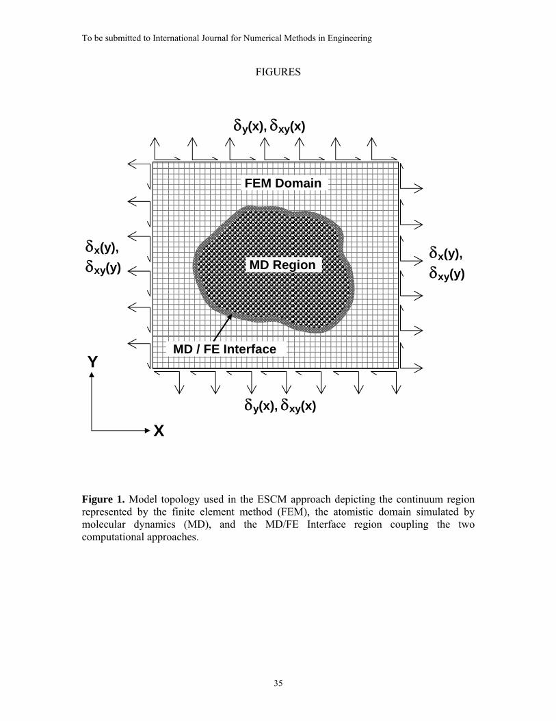
To be submitted to International Journal for Numerical Methods in Engineering
35
FIGURES
Figure 1. Model topology used in the ESCM approach depicting the continuum region represented by the finite element method (FEM), the atomistic domain simulated by molecular dynamics (MD), and the MD/FE Interface region coupling the two computational approaches.
δy(x), δxy(x)
δx(y), δxy(y)
δy(x), δxy(x)
δx(y), δxy(y)
FEM Domain
MD / FE Interface
X
Y
MD Region
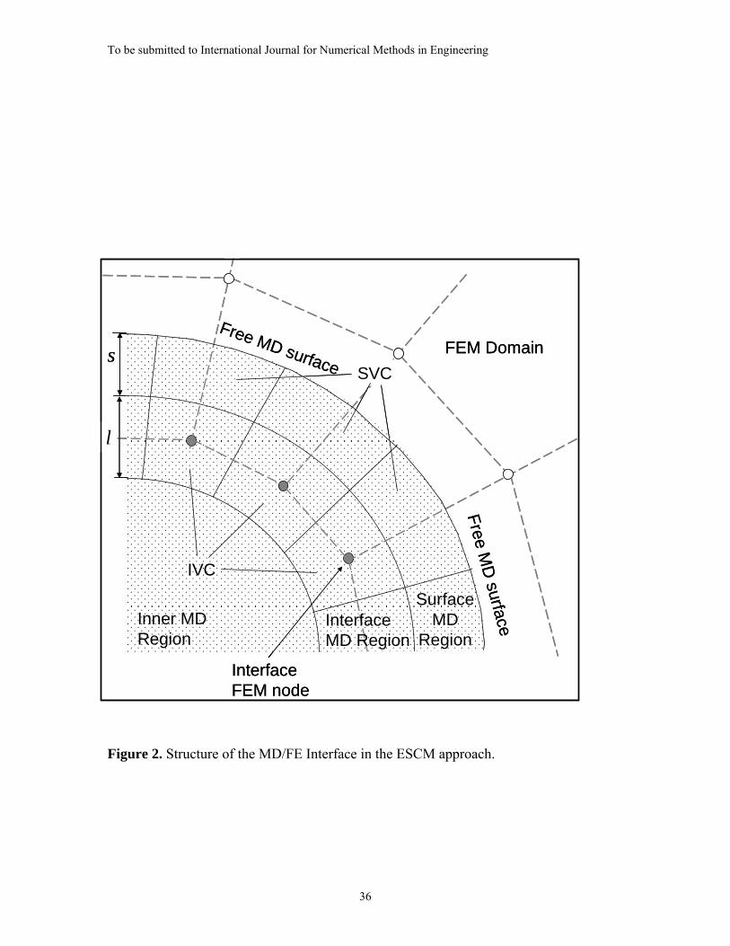
To be submitted to International Journal for Numerical Methods in Engineering
36
Figure 2. Structure of the MD/FE Interface in the ESCM approach.
Inner MD Region
IVC
SurfaceMD
Region
Free MD
surface
Interface FEM node
FEM Domain
Interface MD Region
l
sFree MD surface SVC
Inner MD Region
IVC
SurfaceMD
Region
Free MD
surface
Interface FEM node
FEM Domain
Interface MD Region
l
sFree MD surface SVC
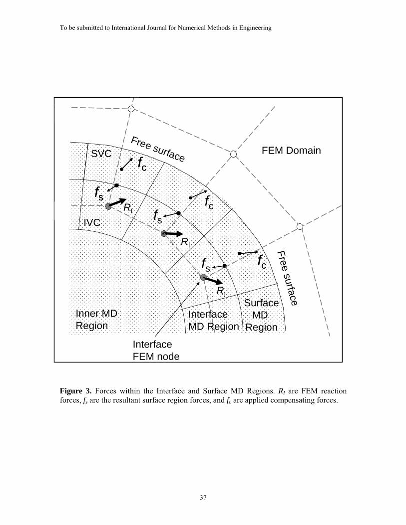
To be submitted to International Journal for Numerical Methods in Engineering
37
Figure 3. Forces within the Interface and Surface MD Regions. RI are FEM reaction forces, fs are the resultant surface region forces, and fc are applied compensating forces.
Inner MD Region
IVC
SVC
SurfaceMD
Region
Free surface
Interface FEM node
fc
fcfc
fcfc
RI
RI
RI
FEM Domain
Interface MD Region
Free surface
fs
fs
fsfs
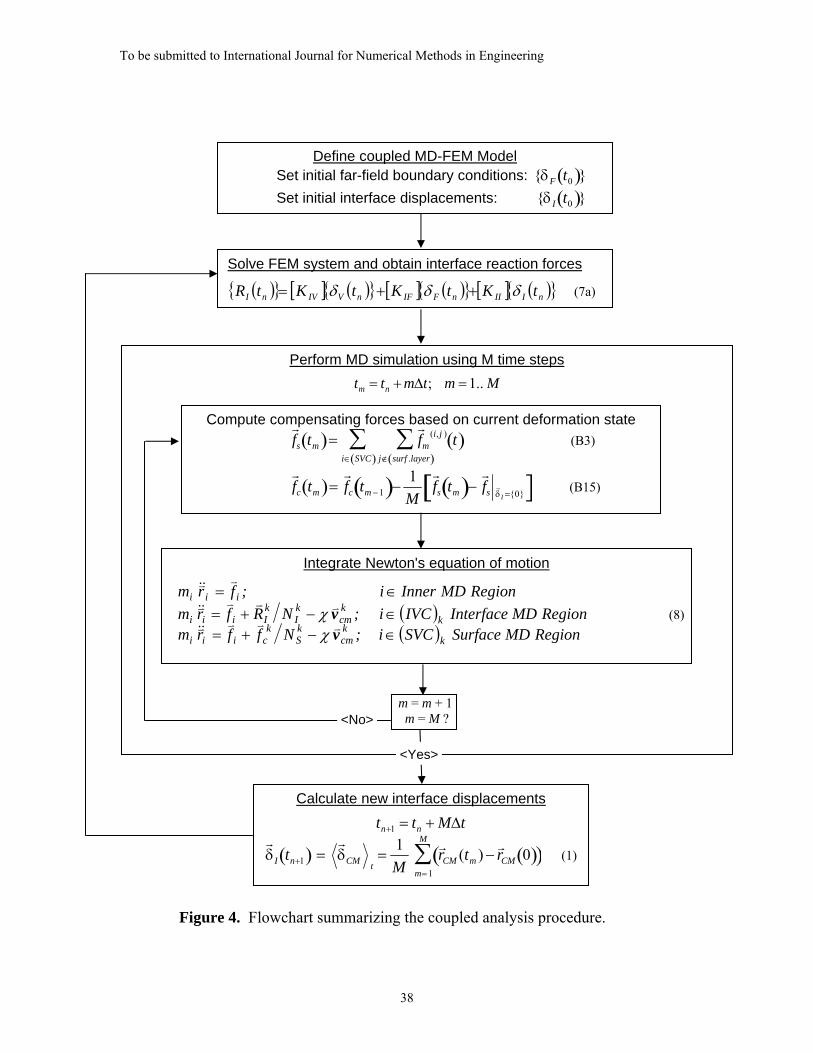
To be submitted to International Journal for Numerical Methods in Engineering
38
Figure 4. Flowchart summarizing the coupled analysis procedure.
Define coupled MD-FEM Model Set initial far-field boundary conditions: {δF t0( )}
Set initial interface displacements: {δ I t0( )}
Solve FEM system and obtain interface reaction forces
( ){ } [ ] ( ){ } [ ] ( ){ } [ ] ( ){ }nIIInFIFnVIVnI tKtKtKtR δδδ ++= (7a)
Perform MD simulation using M time steps tm = tn + mΔt; m = 1.. M
Compute compensating forces based on current deformation state
r f s tm( )=
r f m
(i, j ) t( )j∉ surf .layer( )
∑i∈ SVC( )∑ (B3)
r f c tm( )=
r f c tm −1( )−
1M
r f s tm( )−
r f s r
δ I ={0}[ ] (B15)
Integrate Newton's equation of motion
( )( ) egionRMDSurfaceSVCi;Nffrm
RegionMDInterfaceIVCi;NRfrmRegionMDInneri;frm
kkcm
kS
kciii
kkcm
kI
kIiii
iii
∈−+=∈−+=∈=
vvvvv
&&v
vvv&&v
v&&v
χχ (8)
Calculate new interface displacements
tn+1 = tn + MΔt r δ I tn+1( ) =
r δ CM t
=1M
r r CM (tm ) −r r CM 0( )( )
m= 1
M
∑ (1)
m = m + 1 m = M ? <No>
<Yes>
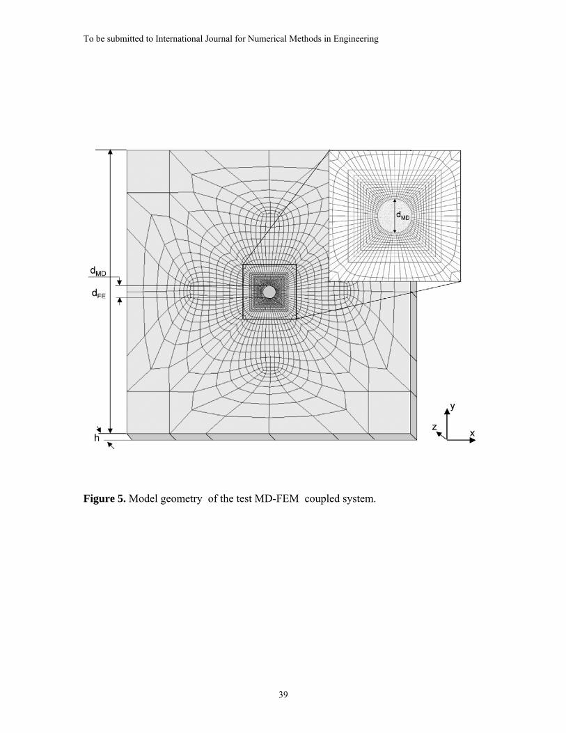
To be submitted to International Journal for Numerical Methods in Engineering
39
Figure 5. Model geometry of the test MD-FEM coupled system.
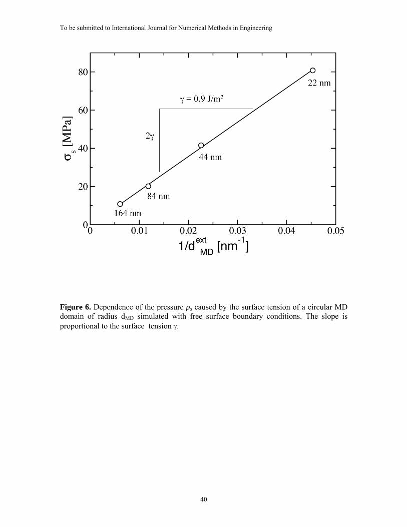
To be submitted to International Journal for Numerical Methods in Engineering
40
Figure 6. Dependence of the pressure ps caused by the surface tension of a circular MD domain of radius dMD simulated with free surface boundary conditions. The slope is proportional to the surface tension γ.
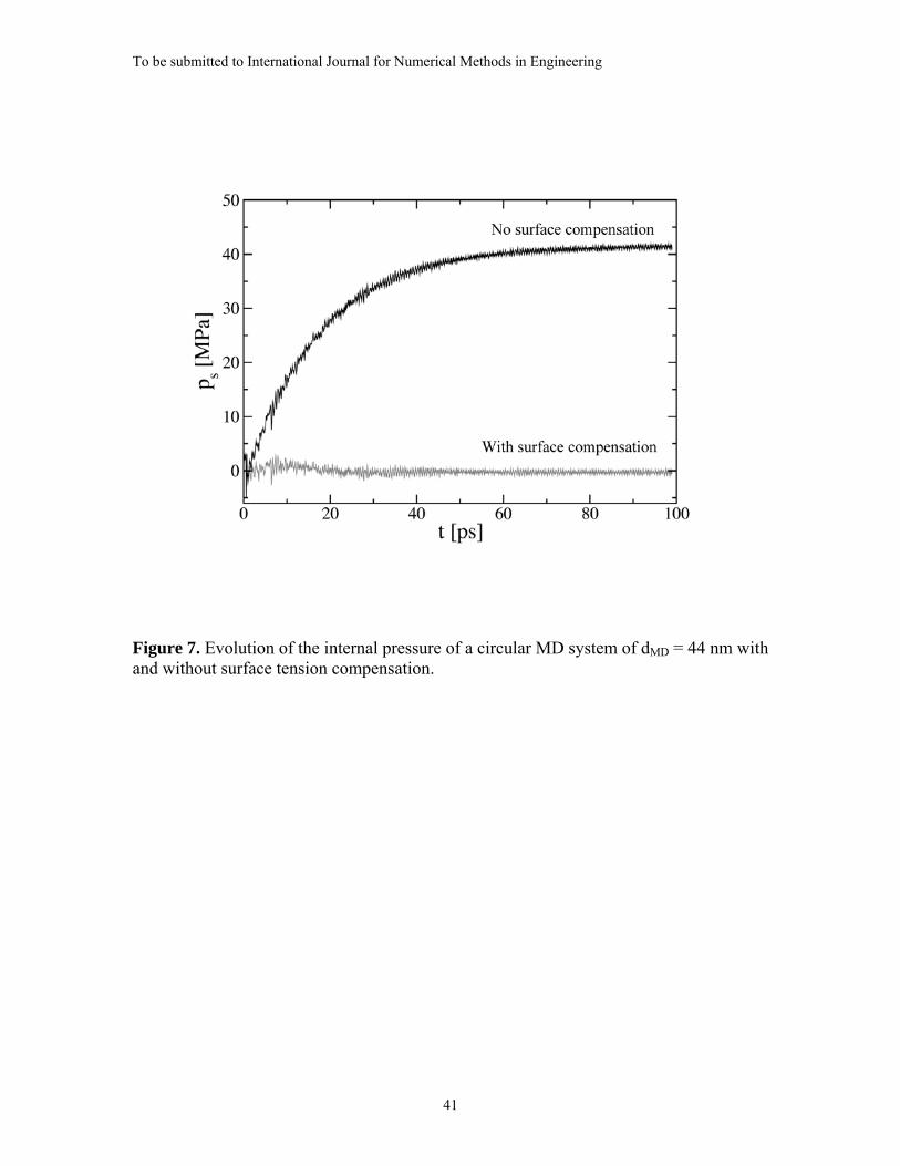
To be submitted to International Journal for Numerical Methods in Engineering
41
Figure 7. Evolution of the internal pressure of a circular MD system of dMD = 44 nm with and without surface tension compensation.
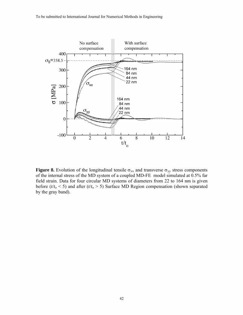
To be submitted to International Journal for Numerical Methods in Engineering
42
Figure 8. Evolution of the longitudinal tensile σxx and transverse σyy stress components of the internal stress of the MD system of a coupled MD-FE model simulated at 0.5% far field strain. Data for four circular MD systems of diameters from 22 to 164 nm is given before (t/to < 5) and after (t/to > 5) Surface MD Region compensation (shown separated by the gray band).
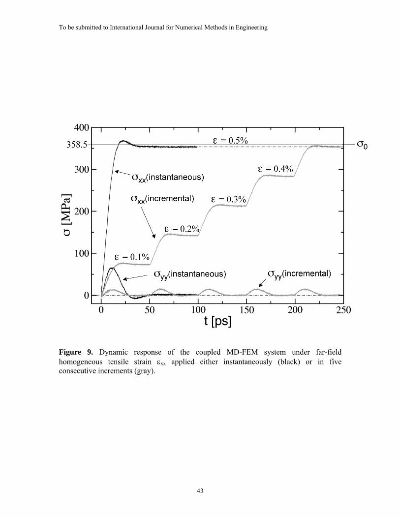
To be submitted to International Journal for Numerical Methods in Engineering
43
Figure 9. Dynamic response of the coupled MD-FEM system under far-field homogeneous tensile strain εxx applied either instantaneously (black) or in five consecutive increments (gray).
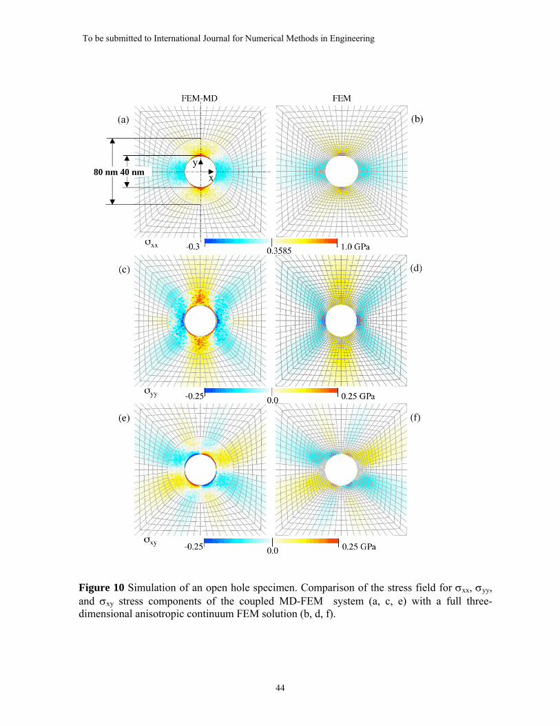
To be submitted to International Journal for Numerical Methods in Engineering
44
80 nm 40 nm
Figure 10 Simulation of an open hole specimen. Comparison of the stress field for σxx, σyy, and σxy stress components of the coupled MD-FEM system (a, c, e) with a full three-dimensional anisotropic continuum FEM solution (b, d, f).
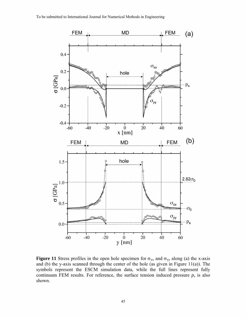
To be submitted to International Journal for Numerical Methods in Engineering
45
Figure 11 Stress profiles in the open hole specimen for σxx and σyy along (a) the x-axis and (b) the y-axis scanned through the center of the hole (as given in Figure 11(a)). The symbols represent the ESCM simulation data, while the full lines represent fully continuum FEM results. For reference, the surface tension induced pressure ps is also shown.
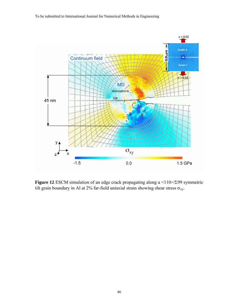
To be submitted to International Journal for Numerical Methods in Engineering
46
Figure 12 ESCM simulation of an edge crack propagating along a <110>/Σ99 symmetric tilt grain boundary in Al at 2% far-field uniaxial strain showing shear stress σxy.
Grain II
Grain I
ε = 0.02
ε = 0.02
0.9
μm
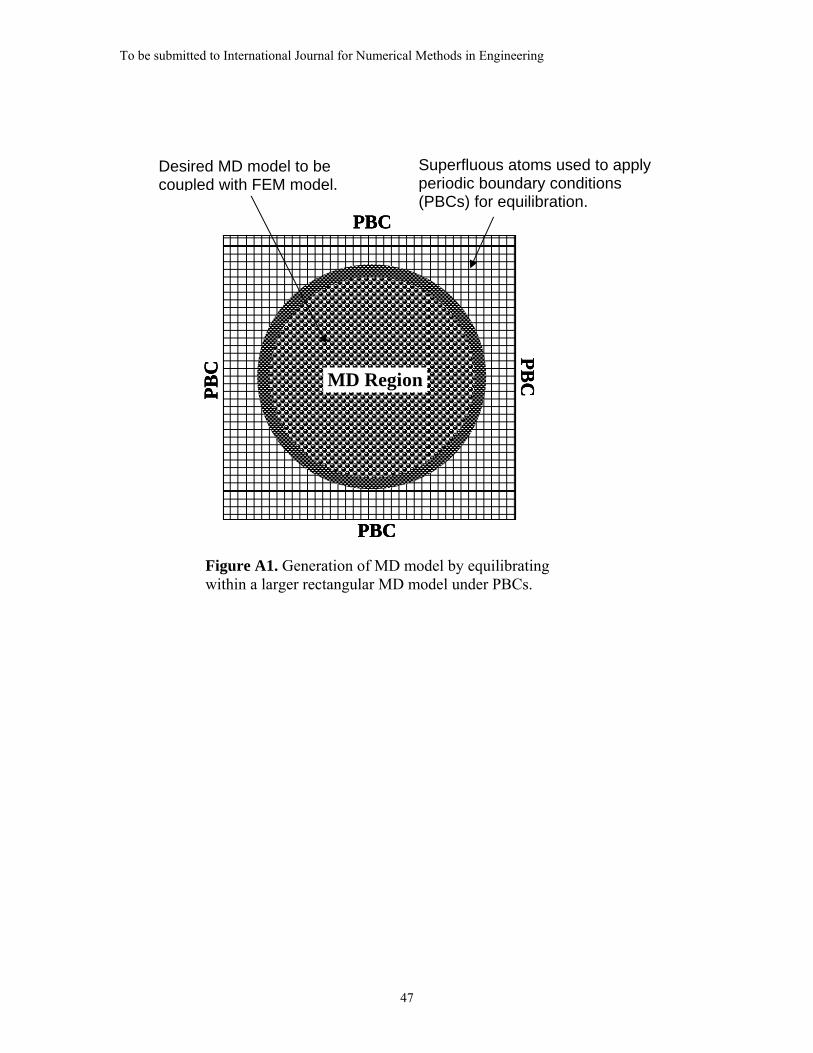
To be submitted to International Journal for Numerical Methods in Engineering
47
PBC
PBC
PBC
PBCMD Region
PBC
PBC
PBC
PBC
PBC
PBC
PBC
PBCMD Region
Desired MD model to be coupled with FEM model.
Superfluous atoms used to apply periodic boundary conditions (PBCs) for equilibration.
Figure A1. Generation of MD model by equilibrating within a larger rectangular MD model under PBCs.
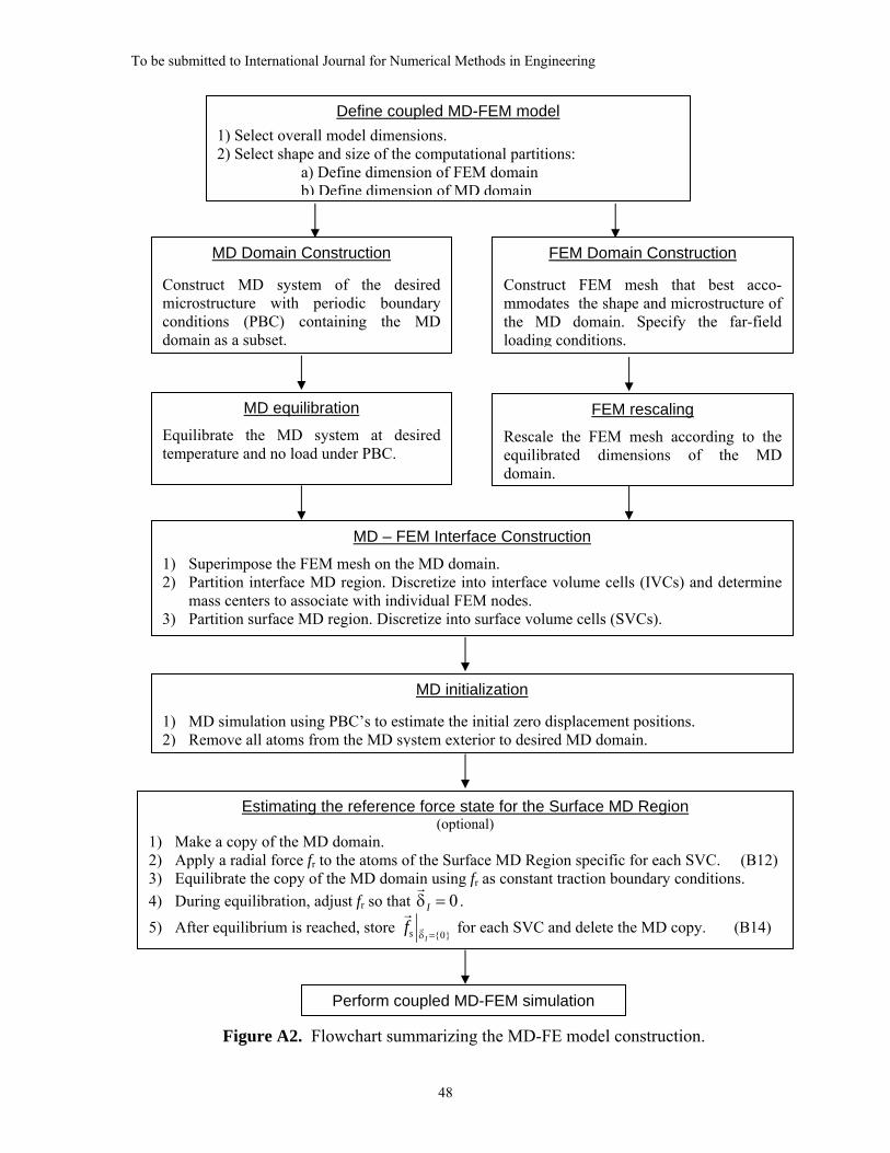
To be submitted to International Journal for Numerical Methods in Engineering
48
Figure A2. Flowchart summarizing the MD-FE model construction.
Define coupled MD-FEM model 1) Select overall model dimensions. 2) Select shape and size of the computational partitions: a) Define dimension of FEM domain
b) Define dimension of MD domain
FEM rescaling Rescale the FEM mesh according to the equilibrated dimensions of the MD domain.
MD equilibration Equilibrate the MD system at desired temperature and no load under PBC.
Perform coupled MD-FEM simulation
MD Domain Construction
Construct MD system of the desired microstructure with periodic boundary conditions (PBC) containing the MD domain as a subset.
FEM Domain Construction
Construct FEM mesh that best acco-mmodates the shape and microstructure of the MD domain. Specify the far-field loading conditions.
MD – FEM Interface Construction 1) Superimpose the FEM mesh on the MD domain. 2) Partition interface MD region. Discretize into interface volume cells (IVCs) and determine
mass centers to associate with individual FEM nodes. 3) Partition surface MD region. Discretize into surface volume cells (SVCs).
Estimating the reference force state for the Surface MD Region (optional)
1) Make a copy of the MD domain. 2) Apply a radial force fr to the atoms of the Surface MD Region specific for each SVC. (B12) 3) Equilibrate the copy of the MD domain using fr as constant traction boundary conditions. 4) During equilibration, adjust fr so that
r δ I = 0.
5) After equilibrium is reached, store r f s r
δ I ={0} for each SVC and delete the MD copy. (B14)
MD initialization
1) MD simulation using PBC’s to estimate the initial zero displacement positions. 2) Remove all atoms from the MD system exterior to desired MD domain.