An Empirical Analysis of Bond Recovery Rates: Exploring a Structural View of Default 1

Daniel Covitz and Song Han

Division of Research and Statistics The Federal Reserve Board

20th and C Streets, NW Washington, D.C. 20551

December 2004

1 We thank Mark Carey, Morris Davis, Darrell Duffie, Michael Gibson, Michael Gordy, Paul Harrison, Erik Heitfield, Nellie Liang, Andrea Sironi, Jonathan Wright, and seminar participants at the Federal Reserve Board for their helpful comments. Daniel Rawner provided excellent research assistance. The views expressed herein are those of the authors and do not necessarily reflect the views of the Federal Reserve Board, its staff, or the Federal Reserve System. Dan Covitz: phone, (202) 452-5267; e-mail, Dan.Covitz@frb.gov. Song Han: phone, (202) 736-1971; e-mail, Song.Han@frb.gov.

2

Abstract

A frictionless, structural view of default has the unrealistic implication that recovery rates on bonds, measured at default, should be close to 100 percent. This suggests that standard “frictions” such as default delays, corporate-valuation jumps, and bankruptcy costs may be important drivers of recovery rates. A structural view also suggests the existence of nonlinearities in the empirical relationship between recovery rates and their determinants. We explore these implications empirically and find direct evidence of jumps, and also evidence of the predicted nonlinearities. In particular, recovery rates increase as economic conditions improve from low levels, but decrease as economic conditions become robust. This suggests that improving economic conditions tend to boost firm values, but firms may tend to default during particularly robust times only when they have experienced large, negative shocks.

Keywords: Recovery rate, default, credit risk model

JEL Classification: G33, G34, G12

3

I. Introduction The credit risk of corporate debt has two components: the likelihood of default

and the recovery rate given default. Understanding the determinants of these risks is

critical for the design and implementation of debt pricing models and risk management-

strategies.2 However, while a number of studies have investigated the empirical

determinants of default risk (e.g., Altman (1968), Ohlson (1980), Zmijeski (1984),

Begley, Ming, and Watts (1996), Shumway (2001), Hillegeist, Keating, Cram, and

Lundstedt (2002), Saretto (2004)), researchers have only recently begun to conduct

comprehensive empirical investigations of recovery rates (e.g., Izvorski (1997), Hu and

Perraudim (2002), Acharya, Bharath, and Srinivasan (2003), Altman, Brady, Resti, and

Sironi (2004), Bris, Welch, and Zhu (2004)). Our analysis also evaluates the empirical

determinants of recovery rates, but extends the literature by linking these determinants to

a structural view of default.

However, by thinking about recovery rates in a structural framework, we

immediately run into the question of why observed recovery rates are so low. Consider,

for example, a model in which the market value of a firm’s assets relative to its liability

level (referred to here as the firm’s inverse market leverage ratio or IMLR) evolves

smoothly over time, and in which the firm defaults immediately when it becomes

insolvent (i.e., when IMLR falls to or below 100 percent).3 In this frictionless

framework, it should be intuitive that recovery rates, particularly when measured at

default, will be close to 100 percent, which fits poorly with the empirical reality that

recovery rates at default (or RAD)—measured by bond price at default as percent of par

value—for nonfinancial corporations over the past two decades have averaged only about

40 percent with a standard deviation of about 28 percent.4

2 For the importance of modeling default risk in bond pricing, see, for example, Merton (1974), Litterman and Iben (1991), Jarrow and Turnbull (1995), Madan and Unal (1998), Duffie and Singleton (1999), and Acharya, Ranjan, and Rangarajan (2002). For the role of recovery rate risk in bond pricing, see, for example, Bakshi, Madan, and Zhang (2001). For the importance of default and recovery risk in credit risk management models, see, for example, Fry (2000b), Carey (2001), and Gordy (2003). 3 Note that RAD and IMLR are not identical concepts. When a firm defaults, RAD is always equal to IMLR. However, for firms that are not in default RAD is not well defined, and expected RAD will not be equal to IMLR. 4 Authors’ calculations based on Moody’s data on defaulted bonds. The data are supplemented with bond price data from Standard and Poor’s and Merrill Lynch.

4

To generate recovery rates less than 100 percent, a structural framework must

include “frictions.” One friction that has been discussed in the bond pricing literature is

that defaults are likely to occur a period of time after a firm becomes insolvent (see, for

example, Leland and Toft (1996) and Duffie and Lando (2001)). Intuitively, default

delays imply that IMLR and thus RAD may be less than 100 percent. Another well-

known friction that also has the potential to lower RAD below 100 percent is “jumps” or

discrete changes in IMLR (see, for example, Zhou (2001) and Wong and Kwok (2003)).

Jumps reflect a sudden change in investors’ views of the value of the firm and its

liabilities, and may be caused by the initiation or resolution of legal challenges, the

revelation of fraud, the implementation of regulatory changes, or, more generally, the

discrete arrival of information about corporate credit quality (possibly because managers

temporarily hide the information). A third friction that could lower RAD below 100

percent is bankruptcy costs. If firms jump into default, the default will trigger a

discontinuous increase in expected bankruptcy costs, which would dampen RAD.

In addition to generating recovery rates that are less than 100 percent, the above

frictions imply that IMLR at default, and thus RAD, varies across different firms. In our

empirical analysis of the variations in RAD, we include firm-level, industry-level, and

macro-level proxies for IMLR as explanatory variables. We also include proxies for

jumps and bankruptcy costs in our specifications. In addition, we look for indirect

evidence of jumps by evaluating whether the empirical relationship between IMLR

proxies and RAD switches from positive to negative as IMLR proxies become high.

These nonlinearities are suggested by the structural view, which highlights the

conditionality of default. More precisely, when IMLR proxies indicate strong financial

health, the fact that the firm defaulted anyway suggests that the firm must have been

struck by a very bad shock that had yet to be reflected in the measured IMLR but that

nevertheless depressed RAD.5

Our analysis is conducted at the bond level with RAD as the recovery rate

measure. Bond price data for firms at default are obtained from Moody’s Investor

Services, and are supplemented with information from Standard & Poor’s and Merrill

5 A similar point is made in Pykhtin (2003). In a theoretical exploration of recovery rates in a structural framework, he argues that recovery rates may be low for high credit quality firms because such firms would likely default only after experiencing a large negative shock to their financial condition.

5

Lynch. We also use the information on the reasons for default from issues of the

Bankruptcy Yearbook and Almanac to create proxies for jumps. The main sample

consists of over 1,300 nonconvertible public bonds issued by U.S. nonfinancial firms that

defaulted between 1983 and 2002, inclusive. The regression sample sizes depend on the

specification, with the smallest sample being about 600 observations. Focusing on

recovery rates at default is reasonable, since such rates are the actual recovery rates for

investors that choose to sell their bonds at the time when an issuer defaults. Indeed,

many investors do sell their bonds at default, as indicated by the active secondary market

for defaulted bonds (see, for example, Altman 2003).6

Our findings break new ground in understanding the determinants of recovery

rates. We find that firm, industry, and macroeconomic proxies for IMLR are

significantly related to RAD, and that the IMLR proxies explain over one third of the

variation in RAD, though none of the coefficients on the bankruptcy cost measures is

significant. We also find direct evidence of jumps. In particular, firms that defaulted due

to the impact of a change in Medicare reimbursement rules in 1997 had substantially

lower RAD than firms that defaulted for other reasons. The effect is robust to controlling

for a host of other firm, industry, and macroeconomic factors. Further, we find that firms

that defaulted because of an accounting fraud also had lower RAD than other firms;

however, the effect is not robust to the inclusion of additional controls. We also find

evidence of the predicted nonlinearities in the relationship between RAD and proxies for

IMLR. In particular, we find bell-shaped relationships between RAD and industry profit

margin, RAD and detrended GDP, and RAD and short-term interest rates.

These findings also complement the results from other studies of recovery rates.

In the most exhaustive study to date, Acharya et al. (2003) analyze recovery rates

measured at default (RAD) and at resolution (RAR), where resolutions include

bankruptcy emergences, liquidations, and out-of-court restructurings. They find that

RAD increases with firm and industry financial performance, bond size, and bond

seniority, and that RAR increases with industry financial performance, bond seniority,

6 A bondholder may want to sell defaulted bonds for a number of reasons. For example, some institutional investors are prohibited from holding defaulted bonds, while others may not want to because of reputational risk. Primary buyers of defaulted bonds include distressed debt funds, vultures, and opportunistic investors.

6

and less time-in-default.7 However, unlike our results, Acharya et al. do not find that

macroeconomic variables are significantly related to RAD, controlling for firm and

industry factors.8 This discrepancy reflects mainly that we use a more comprehensive

data set with one additional recession, and also that we use nonlinear specifications.9

The existence of a macroeconomic factor in recovery rates is an important issue

for the design of credit risk models. Our results not only show that such a factor exists,

they also suggest strongly that the relationship between macroeconomic conditions and

RAD takes a particular nonlinear form. RAD increases as economic conditions improve

from relatively low levels, but it decreases as economic conditions become particularly

robust. As a result, while defaults may be rare during very robust times, recovery rates

may be relatively low. The intuition is that firms may tend to default during particularly

robust periods only when hit by very bad shocks, which in turn depress recovery rates.

This is surprising, since it implies that an idiosyncratic factor (a firm-level jump) affects

the functional form of the relationship between RAD and the systematic factor through

the conditionality of default.

The remainder of the paper proceeds as follows. In Section II, we discuss our

hypotheses and empirical methodology. The sample construction is described in Section

III. In Section IV, we preview our key results with simple univariate statistics. The

results from our empirical analysis are then presented in Section V, and we conclude in

Section VI.

7 The results in Izvorski (1997), a smaller-scale study of RAR, were similar to Acharya et al.’s RAR results. A number of earlier analyses also show the importance of bond seniority and security for recovery rates. See, for example, Altman and Kishore (1996), Brady (2001), Carty and Hamilton (1999), Franks and Torous (1994), Frye (2000a), Gupton, Gates, and Carty (2000), Hu and Perraudin (2002), and Tashjian, Lease, and McConnell (1996) . 8 Consistent with our results, Thorburn (2000), using a sample of small Swedish firms, finds that macroeconomic factors are important determinants of bond recovery rates. 9 Although not motivated by a structural view of default, we also run regression (not reported) with aggregate default rates. We find that such rates are significant determinants of RAD. This is consistent with the findings in Altman et al. (2004), using aggregate average recovery rates, and Hu and Perraudim (2002), using a relatively limited set of industry controls.

7

II. Hypotheses and Empirical Strategy In this section, we expand our discussion of RAD determinants, present the

empirical strategy, and then discuss the construction of the explanatory variables.

1. Default-Delays, Jumps, and Bankruptcy Costs

In contrast to a “frictionless” structural framework, when firms become insolvent

they are not likely to default immediately on their obligations. The intuitive implication

of introducing this friction into a structural view of default is that RAD may be less than

100 percent and will be equal to IMLR at default. A delay period between insolvency

and default is plausible for two reasons. First, it is allowable under the U.S. bankruptcy

code;10 second, as shown in previous studies (for example, Leland and Toft (1996) and

Duffie and Lando (2001)), firms are likely to take advantage of the delay option in order

to avoid incurring the costs associated with default and/or bankruptcy (such costs are

discussed below).

It is also possible that there are negative “jumps” in a firm’s IMLR, which propel

the firm into insolvency and default and so depress RAD. As already noted in the

introduction, the notion of jumps is not new. Jumps may be caused by an increase in

liabilities due to a change in the expected or actual outcome of litigation or a decrease in

asset values due to a revelation of fraud or a change in regulation. Jumps may also occur

because of the discrete and lumpy arrival of information. From the perspective of

investors, information about company credit quality nearly always arrives in discrete

increments, typically coming in formal announcements from company management or

SEC filings.

A third friction that could be introduced into a structural framework is costs

related to default and/or bankruptcy. Defaults might trigger contract covenants and

capital market restrictions, and perhaps most importantly, liens on a firm’s assets, thereby

disrupting the firm’s operations. Defaults might also tarnish the firm’s reputation for

repaying debt. Further, to the extent that defaults trigger bankruptcy, they may create 10 Of course, insolvency and default are closely related. If a firm is observably insolvent, creditors have the right under the U.S. bankruptcy code to petition the courts for “involuntary” bankruptcy; and, if such petitions are successful, the firm would be in default (see, U.S. Bankruptcy Code Title 11, ch 1, section 101 (32) and Senate report No. 95-989).

8

additional costs.11 For example, a bankrupt firm may not be able to easily pursue

profitable investment opportunities, as all corporate decisions must be vetted by the judge

and the creditors, and the process drains management resources of the firm. In addition,

bankruptcy proceedings themselves generate legal fees, though estimates of these fees in

the literature are small (see, for example, Warner (1977), Weiss (1990), and LoPucki and

Doherty (2004)). These costs are part of IMLR. Thus, if IMLR evolves smoothly, these

costs by themselves are not sufficient to allow for IMLR less than 100 percent at default.

However, for firms that jump into default, such costs would come suddenly, and so

would exacerbate the size of the jump.

In our empirical analysis, we include a number of proxies for IMLR, including

firm-level financial variables, industry and macroeconomic conditions, as well as proxies

for jumps and bankruptcy costs. The theoretical relationship between RAD and IMLR is

positive.12 However, the empirical relationship between RAD and observed IMLR

proxies may be nonlinear. That is, if a firm appears to have a high IMLR, but

nonetheless defaults, then we can infer the existence of a missing negative component of

IMLR. Indeed, a very high observed IMLR proxies may signal an omitted negative jump

in IMLR. As a result, we may observe that recovery rates increase with IMLR proxies

when such proxies are in the “usual” range, but may actually be lower when the proxies

are very high, creating a bell-shaped pattern between RAD and the IMLR proxies. The

precise nature of the nonlinearity is, of course, an empirical question.

The possibility of omitted components of IMLR at default is plausible given the

difficulties of measuring IMLR. The difficulties include the lack of a direct measure of

the market value of a firm’s assets, the fact that balance sheet measures of assets are

recorded at book values and thus inherently backward looking, the fact that stock prices,

while forward looking, are essentially zero at default, the fact that balance sheet data tend

11A default may also result in a firm becoming bankrupt. A default may lead to a voluntary bankruptcy, if the firm seeks protection from its creditors, or it may lead to an involuntary bankruptcy, if creditors believe their claims would be better protected by the bankruptcy courts. 12 This prediction is not unique to structural models, since the proxies for IMLR, except for jump variables, are nearly identical to the variables that have been included in other studies of recovery rates (see, for example Acharya et. al 2003). The value of thinking about recovery rates in a structural framework is that it highlights the role of specific frictions and suggests a likely functional form in the relationship between IMLR proxies and RAD.

9

to only be available in the quarter prior to default, and the possibility that jumps may not

be reflected immediately in a firm’s financial variables.

2. Empirical Strategy

Our empirical strategy is to first estimate the relationship between recovery rates

and proxies for IMLR, ignoring the possibility of jumps and nonlinearities. We also

include variables indicating bond seniority and security. To the extent that the absolute

priority rules hold, even loosely, RAD may increase with bond seniority and security.

This “benchmark” specification, shown below in equation (1), facilitates comparisons

with prior research. In (1) Xt refers to firm, industry, and macroeconomic proxies for

IMLR; COST refers to default and bankruptcy cost components of IMLR; and SDUM

refers to a set of dummy variables for seniority and security.

1 2 3t t t t tR X COST SDUMα β β β ε= + + + + (1)

We next augment the benchmark specifications by allowing the intercept to shift

with indicators of different types of jumps, denoted below as JDUM in equation (2).

1 2 3 4t t t t t tR X COST SDUM JDUMα β β β β ε= + + + + + (2)

We then test for nonlinear relationships between recovery rates and IMLR by

including quadratic terms for the proxies for IMLR, as shown below in equation (3).

2

1 2 3 4 5t t t t t t tR X COST SDUM JDUM Xα β β β β β ε= + + + + + + (3)

Importantly, since our data consist of only defaulted bonds, the coefficients are

biased estimates of the relationship between IMLR proxies and a “latent” recovery rate

which is not conditional upon default. However, the coefficients are unbiased estimates

of what interests us here, which is the relationship between observed proxies for IMLR

and recovery rates conditional upon default. Our interest in “conditional” recovery rates

10

stems from their use as critical inputs into credit risk management models (see, for

example, Pykhtin (2003)).

One additional, potential concern with our approach is that there may be liquidity

and strategic defaults in our sample. These defaults tend to have high recovery rates and

might be correlated with the explanatory variables in our models. While we cannot

identify these defaults, they are more likely to be cured or be resolved through out-of-

court restructuring than to end up in bankruptcy. For this reason, we also report results

(in the robustness section) for models estimated on the samples that exclude defaults that

were cured or resolved through out-of-court restructurings.

All of our models are estimated at the bond level using ordinary least squared

regressions. We use Huber/White methods to compute the robust standard errors of the

coefficients and also allow for correlations between debt instruments by the same issuer.

The construction of the explanatory variables is provided in the next section.

3. Explanatory Variables

Firm, Industry, and Macroeconomic Variables.

The first set of proxies for IMLR includes standard financial ratios constructed

using firm balance sheet and income statement variables. Specifically, we consider the

firm’s inverse book leverage ratio or IBLR (i.e., assets over liabilities), asset tangibility

(tangible assets over total assets), and profit margin (income before interest, taxes,

depreciation and amortization over sales).13 The inclusion of firm leverage and asset

tangibility is also motivated by its potential effect on bankruptcy costs, as discussed

below. IMLR might also be higher, ceteris paribus, when a firm’s industry is particularly

profitable, in so far as such profitability indicates favorable demand shocks, which could

boost the firm’s market values. Therefore, we consider industry-level versions of the

firm-level financial ratios (that is, industry IBLR and profit margin), as well as an

industry market-to-book ratio and an industry current ratio—current asset to total asset

ratio.14 The industry market-to-book ratio is a standard measure of growth opportunity,

13 We also use alternative measures of profitability such as return on assets and sale growth rate. The results using these measures, not shown, are similar to those reported here. 14 We do not include firm level versions of these variables, since their inclusion would greatly reduce sample sizes. Our key qualitative results are robust to the inclusion of these variables.

11

and the industry current ratio measures the degree of industry liquidity, which often

reflects robust profit growth. Both firm and industry variables are obtained from

Compustat. All industry variables are the median values for firms with the same 2-digit

SIC codes. In addition, we include in our specifications a dummy variable for whether a

firm is in the energy or utility industries. Firms in these industries tend to have

substantially higher recovery rates than other firms (as shown in, for example, Acharya

et al. (2003)). In our analysis, we do not attempt to explain this phenomenon, but we do

test the robustness of our results to dropping these firms from our sample.

In addition to firm and industry variables, a firm’s IMLR might, ceteris paribus,

be boosted by favorable macroeconomic conditions. We measure macroeconomic

conditions with real GDP growth rate, detrended real GDP, a short term interest rate (3

month T-Bill rate), and the slope of the interest-rate term structure or “term premium”

(the seven-year Treasury yield less the three-month Treasury yield). Data on the real-side

of the macro economy are from the BEA web site, and data on the financial side are from

the Federal Reserve Board’s public website. Moreover, because we are interested in

contemporaneous relationship between RAD and its potential factors, we use data as

close as possible to the time of default. Specifically, firm variables are for the end of the

quarter immediately before the default, and industry and macroeconomic variables are for

the end of the quarter of default.

Jump Variables

We consider three proxies for jumps in IMLR. The first proxy is an indicator

variable for whether a bankruptcy was caused, in whole or in part, by accounting

improprieties and fraud. The second proxy is an indicator for bankruptcies caused, in

whole or in part, by various torts, including product liabilities (e.g., asbestos), regulatory

and environmental problems (e.g., water contamination), labor relations, pension

disputes, lawsuits related to patent, contracts, and personal injuries. By definition, the

revelation of fraud usually occurs without warning. In contrast, the outcome of torts may

be anticipated well before the eventual default and bankruptcy, thus their impacts may

have been gradually incorporated into the firm’s performance measures. Therefore, the

effect of a fraud on RAD may be easier to detect than the effect of a tort, after controlling

12

for firm IMLR proxies. Data identifying whether defaults were due to frauds or torts are

obtained from annual publications of the Bankruptcy Yearbook and Almanac. The

information is cross-checked with and supplemented by the data collected by Lynn M.

LoPucki’s Bankruptcy Research Database (WebBRD).15 The list of the firms whose

bankruptcies were caused by either frauds or torts is shown in Table A1 of the Appendix.

Our third proxy for jumps in IMLR is an indicator variable for healthcare

companies that defaulted as a result of the Balanced Budget Act of 1997 (BBA). The Act

introduced sweeping reforms to the Medicare programs, and substantially reduced the

cash flows of healthcare providers that relied heavily on Medicare reimbursements.16

The information linking individual defaults to BBA is obtained from Moody’s annual

reports. A list of firms with BBA-induced defaults is shown in Table A in appendix.

Note that most of these defaults occurred in 1999, and some even took place in 2000. On

the one hand, the time lag between the enactment of the Act and actual default is

suggestive of default delays. On the other hand, it is because the Act was not fully

implemented until late 1998 and 1999 (see, for example, Silversmith (2000)).

Bankruptcy Cost Variables

We construct three proxies for bankruptcy costs. The first is the number of

creditor classes, which is approximated by the number of bond classes. The set of

possible bond classes includes senior secured, senior unsecured, senior subordinated,

subordinated, and junior subordinated. The second variable is total assets (in real dollar

and in log). Bankruptcies with more creditor classes and for larger firms may be more

complex. Complex bankruptcy cases may take more time—potentially generating greater

fees for attorneys and investment banks and causing more lost opportunities for the firm.

15 The WebBRD is compiled by Lynn M. LoPucki, a law professor at the University of California at Los Angeles. The Database contains over 600 large cases of public companies that filed for bankruptcy since October, 1980. Its information is collected from bankruptcy court filings, SEC filings, and news stories. For details, see http://lopucki.law.ucla.edu/index.htm. 16 Among the many changes included in the BBA legislation, the major provisions include a reduction in the payment rate of Medicare reimbursements and the establishment of a new prospective payment system to reduce overpayments. The Act had the most severe impact on the companies that provided inpatient hospital services and post-acute care services, including home-health care and skilled-nursing facilities (see Wilensky (2000)). It also appears that the deterioration in financial condition due to BBA led to substantial write-downs in the value of companies’ intangible assets, reportedly as relationships with medical practices unwound with the declines in financial health.

13

In addition, in more complex cases bond values at emergence from bankruptcy may be

relatively variable, which would lower the risk-adjusted value of bonds at default. A

third variable is the firm’s tangible assets to total asset ratio. Bankruptcy costs would

decrease with asset tangibility, since the value of tangible assets may be less adversely

affected by the bankruptcy process than other liquid assets, perhaps because company

employees may easily drain more liquid assets during the bankruptcy process.

Proxies for APR

We construct dummy variables for whether the debt is senior secured, senior

unsecured, and senior subordinated. The omitted category combines subordinated and

junior subordinated bonds as the number of junior subordinated bonds in our sample is

small.

III. RAD Data Our main data on recovery rates are from Moody’s Default Risk Services (DRS).

The DRS data contain information on over 3,000 public bonds that defaulted since 1970.

Moody’s defines a bond as being in default if the obligor either fails to make a scheduled

payment of interest or principal, files for bankruptcy, or carries out a distressed

exchange.17 For defaulted bonds, DRS provides the issuance date, maturity, coupon,

seniority, date of default, type of default, type of resolution, and bond prices (as a percent

of par value) at the end of the default month.18 We use these prices at default (RAD) as

our measures of recovery rates.

For our analysis, we keep only non-convertible public bonds issued by

nonfinancial U.S. firms that defaulted between 1983 and 2002. We also drop the

observations with missing RAD values, but add them back if price data are available

17 A distressed exchange occurs when the issuer offers bondholders a new security or a package of securities that amount to a diminished financial obligation, and/or when the exchange has the apparent purpose of helping the borrower avoid missing a payment, delaying a payment, or filing for bankruptcy. Note that the above definition of default does not include technical defaults such as covenant violations. See Moody’s (2004) for details on technical defaults. 18 The majority of the prices represent actual bids (not necessarily trades) on the defaulted securities. Moody’s obtains the bond price data from Interactive Data Corp., Bloomberg, and Reuters (see Moody’s (1999, 2004)).

14

from either Merrill Lynch’s bond price database or S&P’s CreditPro database. The

resulting sample contains about 650 firms, with 1350 bonds. The mean RAD for these

bonds is 40 percent with standard deviation of 28 percent. Table A2 shows summary

statistics for RAD and all explanatory variables for both the overall sample and the main

regression sample.

IV. Univariate Results In this section we preview two of our key results, using simple univariate sample

statistics. The first result is a generally positive but nonlinear relationship between RAD

and favorable macroeconomic conditions. The second result is a negative relationship

between jumps and RAD.

1. RAD and Macroeconomic Conditions

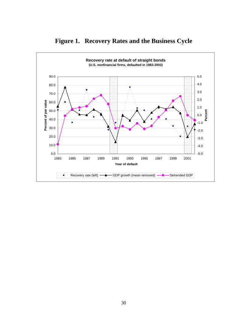
Figure 1 plots annual recovery rates (left scale) against two commonly-used,

annual measures of macroeconomic conditions (right scale) from 1983-2002. The figure

highlights, with shaded regions, the NBER-defined recession periods: July 1990-March

1991, and March 2001-November 2001. The series in the figure are denoted as follows:

the diamonds represent the weighted average RAD of nonfinancial straight bonds by

default year (using defaulted amounts as weights); the triangles denote the deviation of

annual real GDP growth rate from its mean of 3.3 percent; and, the dots indicate the

percentage deviation of annual real GDP from its trend (trend GDP is calculated using

Hodrick-Prescott filter).

Aggregate recovery rates appear cyclical at times, except that they are very low in

particularly robust periods. The average RAD for recession periods was 31 percent,

while the average for expansion periods was 42 percent. However, the lowest average

annual RAD of 20 percent was in 2000—a year of robust economic growth.19 This

nonlinearity dampens the generally positive relation between recovery rates and

macroeconomic conditions. Indeed, the correlation between RAD and real GDP growth

19 According to NBER business cycle dates, the peaks of the two cycles were reached in July 1990 and March 2001, respectively.

15

is just 0.2, and the correlation between RAD and detrended GDP is -0.4.20 This confirms

the weak correlations found in previous papers (for example, Altman et al. (2004) and

Acharya et al. (2003)), and suggests that the empirical relationship between RAD and

macroeconomic variables may be nonlinear.

2. RAD and Jumps

Table 1 shows the unconditional relation between RAD and our three proxies for

jumps in IMLR. Each row shows four statistics of RAD—mean, standard deviation,

median, and sample size—of a particular group of defaults. The first three rows show

these statistics for defaults that were caused by fraud, torts, and “other” reasons. The

second three rows show these statistics for healthcare firms whose defaults were caused

mainly by BBA, “other healthcare” firms, and non-healthcare firms. The last row of the

table (row 7) shows the statistics for all 1346 bonds.

The table shows that RAD on the bonds of firms that defaulted due to fraud and

BBA tended to be lower than RAD on other bonds. The average RAD in the fraud group

is 32 percent (row 1), which is 7 percentage points lower than the average RAD in the

“other” group (row 3). The difference is statistically significant (t=2.25). Surprisingly,

the average RAD in the tort group is significantly higher than that in both the fraud group

and the “other” group.

For the BBA measure, the average RAD in the BBA-healthcare group is 12

percent, which is significantly less than the roughly 40 percent average RAD observed in

both the “other healthcare” group and the non-healthcare group. The pattern of median

RADs across groups is similar to the pattern of average RADs just discussed.

V. Multivariate Analysis This section presents results from our multivariate analyses of RAD. We begin

with results from a set of “benchmark” specifications. These specifications are similar to

20 The unusually high recovery rates in 1987 and 1993 also contribute to the weak correlations. The high recovery rate in 1987 can be traced to the defaulted bonds of Texaco Co, which filed for bankruptcy due to litigation, and to two other energy firms, Yankee Companies, Inc. and Getty Oil International N.V.. The high recovery rate in 1993 was due to Mesa Inc., an energy firm, and Thermadyne Holdings Corporation, a technology firm.

16

those used in previous research, and so are used to test the robustness of previous results.

We next present results from the specifications that include proxies for jumps in IMLR.

We then show results from the specifications that build on the jump models by including

squared terms of the firm, industry, and macro-level factors. Our final set of results

establishes the robustness of the main results to the use of additional control variables and

different samples.

1. Benchmark Specifications

The benchmark specifications include firm, industry, and macro level factors as

proxies for IMLR, as well as dummy variables for the seniority and security of the debt

instruments, and proxies for the complexity of the firm’s capital structure. All

benchmark specifications are linear in IMLR determinants and exclude the proxies for

IMLR jumps to facilitate comparisons with previous research. We estimate three

specifications (shown in columns 1-3 of Table 2), which differ only in terms of their

macro-level variables. All samples contain 624 observations.

The results from the benchmark specifications provide evidence of firm, industry,

macroeconomic, and bond-level determinants of RAD. Consider first the results for the

firm-level variables, shown in the first three rows of Table 2. The coefficients on firm

inverse book leverage ratio (IBLR) are negative but statistically insignificant in all three

specifications. The coefficients on the firm’s tangible asset ratio are significant (at the 95

percent level) in all three specifications, but the point estimates are negative, which is

puzzling. However, (as we show later in the robustness section) the coefficients on the

firm’s tangible asset ratio become insignificant when industry fixed effects are included

in the specifications. The coefficients on the firm’s profit margin are all positive, and

they are statistically significant in the first two specifications (at the 90 percent level),

with point estimates indicating that a one percentage point increase in firm profit margin

leads to about a one-half percentage point increase in RAD. 21

21 We also experimented with several alternative measures of firm profitability and growth potentials: return on assets, sale growth rate, and market-to-book ratio. The results with the first two are much similar to those reported here. Including firm’s market-to-book ratio reduces the sample size by more than a third. Its coefficient is positive but not statistically significant. Results on all other variables are not materially different. See details in Section V.4.

17

Now consider the impact of industry-level variables on RAD. The coefficients on

industry IBLR are all surprisingly negative, and are significant in the first two

specifications. However, as we show in the later regressions, these coefficients become

insignificant with the inclusion of additional controls. The coefficients on both the

industry market-to-book ratio and the industry current ratio are all positive, as expected,

but they are mostly insignificant. The coefficients on the industry profit margin are all

positive and significant, with the point estimates indicating that a one percentage point

increase in industry profit margin leads to about a 40 basis point increase in RAD. The

coefficients on the dummy variable for whether the bond was issued by a firm in the

energy or utility industry are all significant (at the 95 percent confidence level), with

point estimates suggesting that RADs for such firms are at least 22 percentage points

higher, ceteris paribus, than RADs for other firms. The higher level of recovery rates on

bonds issued by energy and utility firms is well known, and we have little to say about

why this is the case. However, we do test and find (not shown) that our results are

similar if we estimate the regressions without energy and utility firms.

We also find evidence in these benchmark specifications that some macro-level

proxies for IMLR are significant determinants of RAD. While the coefficients on the real

GDP growth rate and detrended real GDP, as shown in columns 1 and 2, are not

significant, those on the 3-month T-Bill yield and term premium, as shown in columns 3,

are significant (at the 90 and 95 percent confidence levels, respectively) with the

expected positive signs. The point estimates indicate that a one percentage point increase

in the 3-month Treasury yield increases RAD by about 4 percentage points, and that a

one percentage point increase in term premium increases RAD by about 3 percentage

points.

The results from the benchmark specifications confirm the effect of bond

seniority on RAD found in previous studies. The coefficients on the dummy variable

indicating that the bond is senior secured are positive and significant (at the 95 percent

confidence level) in all three specifications, as are the coefficients on the dummy variable

indicating that the bond is senior unsecured. In addition, the point estimates show that

the economic impact of seniority is large: RAD on senior secured bonds, ceteris paribus,

is roughly 28 percentage points higher than on junior subordinated and subordinated

18

bonds (the omitted categories), and RAD on senior unsecured bonds, ceteris paribus, is

roughly 12 percentage points higher. However, there is no statistically discernable

impact of a bond being senior subordinated relative to other subordinated bonds. The

impact of seniority and security shown here is similar to that found in Acharya et al.

(2003).

With respect to the bankruptcy costs, we find that the coefficients on the measures

of firm complexity (number of classes and log of total assets) are all insignificant. These

results are roughly consistent with prior research, though Acharya et al. (2003) do find a

significant impact of complexity measures on RAD in some specifications.

2. Adding Jumps

Table 3 displays results from six specifications with proxies for negative jumps in

IMLR. The first three specifications (columns 1-3) are the same as in the previous table,

but augmented with three jump proxies: one indicates the default was due to fraud;

another indicates the default was due to a tort; and, the last indicates that default was

caused by the Balanced Budget Act of 1997 (BBA). In the next three specifications

(columns 4-6) we exclude all firm level financial variables from the regressions to boost

the sample size. In the table, we shade the coefficients and standard errors for the

macroeconomic and jump variables. Note that the t tests on the coefficients that proxy

for the jumps may be interpreted as joint tests of whether the variables proxy for jumps,

whether jumps depress RAD, and whether jumps are not already reflected in other

financial information.

The results provide some direct evidence of jumps. We find that RAD for firms

that defaulted due to BBA is significantly lower (at the 95 percent confidence level),

ceteris paribus, than RAD for other firms. The coefficients on BBA dummy variable are

statistically significant at the 95 percent confidence level, and they indicate that RADs on

bonds issued by firms that defaulted due to BBA are between 16 and 22 percentage

points lower, ceteris paribus, than those on other bonds. In contrast, the coefficients on

fraud and tort variables in the first three specifications are surprisingly positive and

statistically significant. However, as shown in columns 4-6, with a larger sample (1275

observations) due to the exclusion of firm-level financial variables, these coefficients are

19

insignificant, suggesting that the puzzling effects of fraud and tort may be due to the

sampling.

Comparing columns 1-3 in Table 3 to those in Table 2, we find that the inclusion

of jump proxies does not qualitatively affect the coefficients on the firm-, industry-, and

macro-level variables. The notable exception is that the coefficients on industry IBLR

become insignificant. Comparing columns 1-3 in Table 3 to columns 4-6, we find that,

when all firm-level financial variables are excluded from the regressions, the coefficients

on the industry current ratio become significant (at the 95 percent confidence level), with

the point estimates indicating that a one percentage point increase in industry current

ratio leads to a 5 percentage point increase in RAD. The coefficients on detrended GDP

also become significant, but have unexpected negative signs. We show later that this

may be due to the misspecification and that the true relationship appears to be bell-

shaped. The coefficients on industry IBLR are insignificant.

We now turn to our analysis of nonlinear effects.

3. Adding Nonlinear Terms

We test for nonlinearities in firm, industry, and macro IMLR proxies by

augmenting the same six specifications presented in Table 3 with squared terms for the

firm, industry, and macroeconomic IMLR proxies. When presenting the results, shown

in Table 4a, we shade the coefficients for a variable and its squared terms when they are

jointly statistically significant at the 90 percent confidence level.

The results provide substantial evidence of nonlinearities in the relationship

between IMLR proxies and RAD, but the predicted bell-shaped relationship is only

within the “reasonable” range of data for some industry and macroeconomic variables.

By “reasonable,” we mean below the 90th percentile of the sample distribution for the

respective variable. The coefficients on firm IBLR and its squared term are jointly

significant in the first three specifications (at the 90 percent confidence level). Moreover,

because the coefficient of the squared term is negative, the relationship between RAD

and firm IBLR appears to be bell-shaped: RAD initially increases with firm IBLR but

decreases when firm IBLR is over certain level. However, the point estimates indicate

that the top of the bell occurs outside of the “reasonable” range of the data—firm IBLR

20

would have to be over 27 (or 2,700 percent) before the total marginal effect would lead to

a decrease in RAD. Thus, RAD is essentially increasing in firm IBLR within the range of

the data. The coefficients on the firm’s tangible asset ratio and its squared term are

jointly significant, and the coefficients on the firm’s profit margin and its squared term

are jointly significant in one of the three specifications. However, as with firm IBLR, the

point estimates indicate that the turning points of the two curves are both outside of the

“reasonable” data range. As a result, in the reasonable range of the data, RAD is

decreasing in the firm’s tangible asset ratio and increasing in the firm’s profit margin.

But, as we show later, both relationships are also not robust.

We next consider the coefficients on the industry variables. The coefficients on

the industry inverse book leverage and its squared term are significant in the regressions

with firm variables excluded (columns 4-6). But the turning point of the bell occurs

outside of the “reasonable” data range (at about the 98th percentile of its sample

distribution), suggesting that RAD is essentially increasing in industry IBLR. The

coefficients on the industry profit margin and its square term are jointly significant in all

six regressions. Moreover, the negative coefficients on the squared terms do suggest a

bell-shaped relationship within the reasonable range of the data, with point estimates

indicating that the top of the bell is around an industry profit margin of 18 percent (at

about the 82nd percentile of its sample distribution). Such a bell-shaped relationship also

exists for industry current ratio in the regressions with firm variables excluded (columns

4-6).

Similar bell-shaped nonlinear relationships are also found for macroeconomic

variables. For detrended GDP, its linear and squared terms are jointly significant.

Moreover, the point estimates indicate that the total marginal effect is essentially

increasing in detrended GDP when it is negative, but decreasing when it is positive (the

top of the bell is at about 0.13 percent). A statistically significant bell-shaped pattern

within the “reasonable” data range is also observed for the relationships between the

three-month Treasury yield and RAD.

It is also worth noting that the coefficients of the BBA dummy are still large,

negative, and significant (at the 95 percent confidence level). As in Table 3, the

coefficients on the fraud and tort dummy variables are mostly insignificant.

21

The key concern for credit risk management modeling is the relationship between

RAD and macroeconomic variables. To further investigate this relationship, we estimate

regressions that include only macroeconomic variables and bond seniority and security

dummy variables. We estimate three specifications, which differ only in terms of their

macroeconomic variables, and the results are shown in Table 4b. We find that the

coefficients on all the macroeconomic variables and their respective squared terms are

jointly statistically significant. In addition, nearly all the coefficients imply a bell-shaped

relationship between RAD and macroeconomic variables within the “reasonable” range

of the data. For instance, RAD appears to first increase with the real GDP growth rate

but then decrease when the real GDP growth rate is greater than 3.8 percent. The tops of

the bells with respect to detrended GDP and the 3-month Treasury yield are at -0.2

percent and 7.1 percent, respectively. The coefficients on the term premium and its

squared term suggest a cup-shaped relationship, but the bottom of the cup is far outside of

the data range. Thus, RAD is essentially increasing in the term premium. On the whole,

these results provide strong evidence that a macroeconomic factor exists and also suggest

that its relationship with RAD is nonlinear.

4. Robustness

Effects of Firm Market-to-Book Ratio

To evaluate the robustness of the result, we augment the first three specifications

in Table 4a with an additional firm-level variable. The new variable is the firm’s market-

to-book ratio (i.e., the sum of a firm’s market value of common equity and its book value

of assets net of book value of common equity to its book value of assets). This variable

is used in the finance literature as a measure of growth prospects or risk, and thus is a

natural proxy for IMLR. This variable also contains direct information on the market

value of the firm. We excluded it from earlier specifications due to its limited

availability. Indeed, the sample size drops from 624 to 391 when the firm’s market-to-

book ratio is included.

Our main results, shown in Table 5, are similar but not identical to those in Table

4a. With respect to the firm-level variables, only the results in column 2 are similar as

before. All the firm-level variables are insignificant in the other two regressions. With

22

respect to the industry-level variables, only the industry profit margin is significant and

only in column 1. The signs and sizes of the coefficients are close to those in Table 4a.

Turning to jumps, the coefficients on the BBA dummy are significant in two of the three

specifications with similar magnitudes as in Table 4a. The coefficients on the fraud

dummy variable are now insignificant, while the coefficients on the tort dummy variable

are again mostly significant. With respect to macroeconomic variables, we find the same

bell-shaped relationships for detrended real GDP and the 3-month T-Bill yields. In

addition, the relationship between RAD and term premium is now also bell-shaped, and

the top of the bell is at a term premium of 2.3 percent, just above the median of our

regression sample.

Additional Industry Effects

For additional robustness, we augment the specifications in Table 4a with

indicator variables for the telecom, technology and steel industries. These specifications

are motivated by the possibility that the nonlinearities found in the macroeconomic

variables are driven by a spate of telecom and technology defaults with relatively low

RAD.

The results, shown in Table 6, indicate that telecom and steel industry bonds have

lower recovery rates. The coefficients on the telecom dummy variable are all significant

(at the 95 percent confidence level), and they suggest that RADs on telecom bonds are

about 20 percentage points lower, ceteris paribus, than on other bonds (the omitted

category). The coefficients on the steel industry dummy are significant in two of the

three specifications, and they suggest that RADs on steel bonds are about 11 percentage

points lower, ceteris paribus, than on other bonds (the omitted category). In contrast, the

coefficients on the technology industry dummy are insignificant. The point estimates for

energy and utility bonds are similar to those in Table 4a.

However, industry effects do not alter our main results. First, RAD is again

increasing in firm IBLR within the “reasonable” data range. Second, the relationships

between RAD and macroeconomic variables, including detrended real GDP and the 3-

month T-Bill yield, are bell-shaped The same bell-shaped relationship also exists for

23

industry profit margin. Third, RADs for firms that defaulted due to BBA are

significantly lower, ceteris paribus, than for other firms.

Excluding Defaults Cured or Resolved through Out-of-Court Restructurings

We conduct two experiments to analyze the impact of liquidity defaults. First, we

exclude cured defaults from our regression sample. The results, reported in columns 1-3

in Table 7, show that excluding cured defaults reduces the sample size by only 17

observations and has a negligible impact on the results. Second, we exclude defaults that

were resolved through out-of-court restructurings, including non-bankruptcy

reorganizations and distressed exchanges. The results, reported in columns 4-6 in Table

7, show that this reduces the sample size by 65 observations, but has little effect on the

signs and sizes of the coefficients.

VI. Conclusions A structural view of default suggests that variations in bond recovery rates may

reflect “frictions” such as delays between insolvency and default, jumps in firm value,

and cost of default and bankruptcy. Moreover, conditional on default, the empirical

relationship between RAD and proxies for the firm’s inverse market leverage ratio

(IMLR) may be nonlinear. In particular, RAD may increase with favorable proxies for

IMLR when these proxies are in the “usual” range, but may be low when these proxies

are at “unusually” high levels.

Using a comprehensive dataset on bond recovery rate, we find that firm, industry,

and macroeconomic proxies for IMLR are positively and significantly related to RAD,

and they help explain over one third of the variations in RAD. The results are consistent

with the notion that standard frictions, such as default delays and jumps in corporate

valuations, drive RAD below 100 percent. We also find some direct evidence of jumps.

In contrast, we find no evidence that another friction, bankruptcy costs, is a significant

determinant of RAD. Finally, we find nonlinearities in the relationship between

macroeconomic proxies for IMLR and RAD, with RAD increasing as economic

conditions improve from relatively low levels, but decreasing as economic conditions

24

become robust. We argue that these nonlinearities may arise because of the intuitive

possibility that firms may be more likely to default because of a jump during particularly

robust economic times.

Reference

Acharya, Viral V; Das, Sanjiv Ranjan; Sundaram, Rangarajan K. “Pricing Credit

Derivatives with Rating Transitions,” 2002, C.E.P.R. Discussion Papers, CEPR

Discussion Papers: 3329

Acharya, Viral V., Sreedhar T. Bharath, and Anand Srinivasan. A., “Understanding the

Recovery Rates on Defaulted Securities.” Working paper. September 2003.

Altman, E. I.. “Financial Ratios, Discriminant Analysis, and the Prediction of Corporate

Bankruptcy,” Journal of Finance 23:589-609, 1968.

Altman, E.I., “Market size and investment performance of defaulted bonds and bank

loans: 1987-2002,” Journal of Applied Finance. Fall/Winter 2003. 43-53.

Altman Edward I. and Gaurav Bana. “Defaults and Returns on High-Yield Bonds.”

Journal of Portfolio Management. Winter 2004, 58-73.

Altman, E.I., B. Brady, A. Resti, and A. Sironi, 2001, “The link between default and

recovery rates,” Journal of Business.

Altman Edward I. and Eberhart, Allan C. (1994), “Do Seniority Provisions Protect

Bondholders’ Investments?,” A New York University Salomon Center Working Paper;

Seires S-94-12.

25

Bakshi, Gurdip; Madan, Dilip; Zhang, Frank. “Recovery in default risk modeling:

theoretical foundations and empirical applications,” 2001, Board of Governors of the

Federal Reserve System (U.S.), Finance and Economics Discussion Series: 2001-37

Begley, J., Ming, J., and Watts, S.. “Bankruptcy Classification Errors in the 1980s:An

Empiricl Analysis of Altman’s and Ohlson’s Models,” Review of Accounting Studies

1:267-84. 1984.

Bris, Arturo, Ivo Welch, and Ning Zhu. “The Costs of Bankruptcy: Chapter 7 Cash

Auctions vs. Chapter 11 Bargaining.” Yale ICF Working Paper No. 04-13. March 2004.

Carapeto, Maria. A., “Is Bargaining in Chapter 11 Costly?” Cass Business School

Working Paper. October 2003.

Carey, Mark. “Credit Risk in Private Debt Portfolios,” Journal of Finance, August 1998,

v. 53, iss. 4, pp. 1363-87

Carey, Mark. “Dimensions of Credit Risk and Their Relationship to Economic Capital

Requirements,” in Prudential supervision: What works and what doesn't, 2001, pp. 197-

228, NBER Conference Report series. Chicago and London: University of Chicago Press,

Carty, Lea V., D. T. Hamilton, S. C. Keenan, A. Moss, M.l. Mulvaney, T. Marshella, M.

G. Subhas. “Bankrupt Bank Loan Recoveries.” Special Comment, Moody’s Investors

Services, Global Credit Research. June 1998.

Duffie, Darrell and David Lando. “Term Structures of Credit Spreads with Incomplete

Accounting Information,” Econometrica, Vol. 69, No. 3 (May, 2001), 633-664.

Duffie, Darrell and Kenneth J. Singleton. “Modeling Term Structures of Defaultable

Bonds,” The Review of Financial Studies, special 1999 Vol. 12, No. 4, pp. 687-720.

26

Eberhart, Allan C. and Sweeney, Richard J. (1992). “Does the Bond Market Predict

Bankruptcy Settlements?,” The Journal of Finance, Vol. XLVII, No. 3, July 1992.

Eberhart, Alan, William Moore, and Rodney Roenfeldt. “Security Pricing and

Deviations from the Absolute Priority Rule in Bankruptcy Proceedings,” Journal of

Finance 45: 1457-1469. 1990.

Fons, Jerome. “Using Default Rates to Model the Term Structure of Credit Risk,”

Financial Analysts Journal, September/October, 1994, pp. 25-32.

Franks, Julian R. and Walter N. Torous. “An Empirical Investigation of U.S. Firms in

Reorganization,” Journal of Finance 44: 747-770. 1989.

Franks, Julian R. and Walter N. Torous. “A comparison of financial recontracting in

distressed exchanges and Chapter 11 reorganizations.” Journal of Financial Economics

35 (1994) 349-370.

Frye, Jon. “Depressing Recoveries.” Risk Magazine, November 2000, 108-111.

Frye, Jon. “Collateral Damage: A source of systematic credit risk.” Risk Magazine,

April 2000, 91-94.

Gordy, Michael B. “A Risk-Factor Model Foundation for Ratings-Based Bank Capital

Rules,” Journal of Financial Intermediation, July 2003, v. 12, iss. 3, pp. 199-232

Andrade, Gregor and Kaplan, Steven N. “How Costly Is Financial (Not Economic)

Distress? Evidence from Highly Leveraged Transactions That Became Distressed.”

Journal of Finance, October 1998, v. 53, issue 5, pp. 1443-93.

Gupton, Greg M., Daniel Gates and Lea V. Carty. “Bank-Loan Loss Given Default.”

Special Comment, Moody’s Investors Service, Global Credit Research, November 2000.

27

Hamilton, David T., Praveen Varma, Sharon Ou, and Richard Cantor. “Default &

Recovery Rates of Corporate Bond Issuers: A Statistical Review of Moody’s Ratings

Performance, 1920-2003.” Special Comment, Moody’s Investors Services, Global Credit

Research. January 2004.

Hu, Yen-ting and William Perraudin. “The Dependence of recovery and defaults.”

Birkbeck College. Feb. 2002.

Hillegeist, Stephen A., E. K. keating, D. P. Cram, and K. G. Lundstedt, “Assessing the

Probability of Bankruptcy,” working paper, Kellogg School of Management,

Northwestern University. April 2002.

Izvorski, I. A. “Recovery Ratios and Survival Times for Corporate Bonds.” IMF

Working Paper. 1997

Jarrow, Robert A.; Turnbull, Stuart M. “Pricing Derivatives on Financial Securities

Subject to Credit Risk,” Journal of Finance, March 1995, v. 50, iss. 1, pp. 53-85

Leland, H., and K. Toft. “Optimal Capital Structure, Endogenous Bankruptcy, and the

Term St4ructure of Credit Spreads,” Journal of Finance, 51, 987-1019.

Litterman, Robert; Iben, Thomas. “Corporate Bond Valuation and the Term Structure of

Credit Spreads,” Journal of Portfolio Management, Spring 1991, v. 17, iss. 3, pp. 52-64

Lopucki, L. M. and J. W. Doherty, 2004, “The Determinants of Professional Fees in

Large Bankruptcy Organization Cases,” The Journal of Empirical Legal Studies 1, 111-

1142.

Lopucki, Lynn and William Whitford. “Patterns in the Bankruptcy Reorganization of

Large, Publicly Held Companies,” Cornell Law Review 78: 597-618. 1993.

28

Madan, Dilip B. and Unal, Haluk, “Pricing the Risks of Default,” Review of Derivatives

Research, December 1998, v. 2, iss. 2-3, pp. 121-60

Moody’s Investor Services, “Default & recovery rates of corporate bond issuers: A

statistical review of Moody’s ratings performance, 1920-2003,” January 2004.

Ohlson, J. S.. “Financial Ratios and the Probabilistic Prediction of Bankruptcy.” Journal

of Accounting Research 19:109-31. 1980.

Pykhtin, Michael. “Unexpected Recovery Risk.” Risk, August 2003, 74-78.

Saretto, Alessio A.. “Predicting and Pricing the Probability of Default,” working paper,

the Anderson school at UCLA. 2004.

Schuermann, Til. A, “What Do We Know about Loss-Given-Default?” Federal Reserve

Bank of New York Working Paper. March 2003.

Shleifer, Andrei and Robert Vishny. A. “Liquidation Values and Debt Capacity: A

Market Equilibrium Approach.” Journal of Finance, Vol. 47, 1343-1366. 1992.

Shumway, Tyler. “Forecasting Bankruptcy More Accurately: A Simple Hazard Model.”

Journal of Business, 2001, vol. 74, no. 1, 101-124.

Sliversmith, Janet. “The Impact of the 1997 Balanced Budget Act on Medicare.”

Minnesota Medicine. Volume 83, December 2000. Reprinted in the website:

http://www.mnmed.org/publications/MnMed2000/December/Silversmith.html.

Skeel, David A., Jr.. A. “Debt’s Dominion: A History of Bankruptcy Law in America.”

Princeton and Oxford: Princeton University Press. 2001.

29

Tashjian, E., R.C. Lease and J.J. McConnell, 1996, Prepacks: An empirical analysis of

prepackaged bankruptcies, Journal of Financial Economics, 40, 135-162

Wagner, Herbert S. III. "The Pricing of Bonds in Bankruptcy and Financial

Restructuring", Journal of Fixed Income, Putnam Investments (Jun-1996), pp. 40-47.

Warner, Jerold B., “Bankruptcy, Absolute Priority, and the Pricing of Risky Debt

Claims,” Journal of Financial Economics, 1977, Vol. 4, No. 3, 239-276.

Warner, J. A., 1977, “Bankruptcy Costs: Some Evidence,” Journal of Finance 337-347.

Weiss, L., 1990, “Bankruptcy Resolution: Direct Costs and Violations of Absolute

Priority,” Journal of Financial Economics 27, 419-446.

Wilensky, Gail R., “The Balanced Budget Act of 1997: A Current Look at Its Impact on

Patients and Providers,” Statement before the Subcommittee on Health and Environment,

Committee on Commerce, U.S. House of Representatives. July 19, 2000.

Wong, Hoi Ying and Kwok, Yue Kuen, “Jump diffusion models for risky debts: Quality

spread differentials,” International Journal of Theoretical and Applied Finance, Vol. 6,

No. 6 (2003) 655-662.

Zhou, Chunsheng, “The Term Structure of Credit Spreads with Jump Risk,” Journal of

Banking and Finance, November 2001, vol. 25, issue 11, pp. 2015-40.

Zmijewski, M. E.. “Methodological Issues Related to the Estimation of Financial Distress

prediction Models.” Journal of Accounting Research 22:59-82. 1984.

30

Figure 1. Recovery Rates and the Business Cycle

Recovery rate at default of straight bonds (U.S. nonfinancial firms, defaulted in 1983-2002)

0.0

10.0

20.0

30.0

40.0

50.0

60.0

70.0

80.0

90.0

1983 1985 1987 1989 1991 1993 1995 1997 1999 2001

Year of default

Perc

ent o

f par

val

ue

-5.0

-4.0

-3.0

-2.0

-1.0

0.0

1.0

2.0

3.0

4.0

5.0

Perc

ent

Recovery rate (left) GDP growth (mean removed) Detrended GDP

31

Table 1: Recovery Rates and Jumps

(U.S. nonfinancial straight bonds, 1983-2002) --Percent of Par Value--

Reasons for default Mean Std. dev. Median Num. of bonds 1. Fraud 32 25 20 71 2. Tort 52 30 55 156 3. Other 39 27 34 1121 4. BBA-healthcare 12 7 11 14 5. Other healthcare 42 22 48 19 6. Non-healthcare 40 28 35 1315 7. Total 40 28 34 1348 Notes: “Fraud” indicates accounting improprieties; “tort” includes product liabilities, regulatory and environmental problems, labor relations, pension disputes, lawsuits related to patent, contracts, and personal injuries; “BBA-healthcare” indicates the Balanced Budget Act of 1997. Reasons for default are obtained from the Bankruptcy Yearbook and Almanacs and Lynn M LoPucki’s Bankruptcy Research Database (WebBRD).

32

Table 2. Benchmark Regressions of Recovery Rate.

(Non-convertible public bonds by U.S. nonfinancial firms defaulted in 1983-2002) Dependent variable = Recovery rate at default (%)

Independent variables (1) (2) (3) Inverse book leverage -0.01 -0.01 -0.13 (0.12) (0.10) (0.14) Tangible/total assets (%) -0.14* -0.15* -0.15* (0.08) (0.08) (0.08) Profit margin (%) 0.05* 0.05* 0.03 (0.03) (0.03) (0.03) Ind. inverse book leverage -0.79* -0.75* -0.67 (0.40) (0.40) (0.41) Ind. market-to-book (%) 0.04 0.04 0.05 (0.04) (0.04) (0.05) Ind. current ratio (%) 5.59* 5.41 3.64 (3.32) (3.28) (3.22) Ind. profit margin (%) 0.48* 0.48** 0.39* (0.24) (0.23) (0.23) Energy/utility 27.35** 27.47** 21.92** (7.27) (7.11) (6.33) Real GDP growth (%) -0.39 (0.61) Detrended real GDP (%) -1.47 (1.38) 3-month T-bill yield (%) 4.07** (1.08) Term premium (%) 3.22* (1.78) Sr. secured 28.70** 28.34** 36.69** (4.32) (4.42) (4.71) Sr. unsecured 12.35** 12.09** 19.21** (4.19) (4.19) (3.93) Sr. subordinated 3.37 3.80 7.77* (3.94) (3.95) (4.14) Number of classes 0.78 1.20 -0.95 (2.40) (2.37) (2.29) Log(assets) -0.10 -0.19 0.93 (1.12) (1.12) (1.07)

Number of observations 624 624 624 R2 0.28 0.28 0.31

Note: (a) Standard errors, shown in parentheses, are calculated using Huber/White methods and adjusted for correlations between debt instruments by the same issuer. (b) * and ** indicate statistically significant at 90% and 95% confidence levels, respectively. (c) Variable definitions: Inverse book leverage=assets/debt, profit margin=EBITDA/sale, current ratio=current assets/total assets, term premium=the 7-year Treasury yield less the 3-month Treasury yield, “Number of classes” denotes number of seniority and security classes.

33

Table 3. Effects of jumps on recovery rate

(Non-convertible public bonds by U.S. nonfinancial firms defaulted in 1983-2002) Dependent variable = recovery rate at default (%)

Independent variable (1) (2) (3) (4) (5) (6) Inverse book leverage -0.04 -0.04 -0.13 (0.10) (0.09) (0.14) Tangible/total assets (%) -0.19** -0.20** -0.18** (0.07) (0.07) (0.07) Profit margin (%) 0.04 0.04 0.03 (0.03) (0.03) (0.03) Ind. inverse book leverage -0.55 -0.54 -0.53 0.26 0.31 0.27 (0.36) (0.37) (0.38) (0.88) (0.86) (0.85) Ind. market-to-book (%) 0.02 0.02 0.04 0.03 0.03 0.04 (0.04) (0.04) (0.04) (0.04) (0.04) (0.04) Ind. current ratio (%) 1.80 1.75 0.96 5.74** 6.65** 4.73* (3.17) (3.13) (3.11) (2.62) (2.62) (2.77) Ind. profit margin (%) 0.52** 0.51** 0.43* 0.61** 0.72** 0.56** (0.24) (0.23) (0.23) (0.17) (0.17) (0.18) Energy/utility 21.98** 22.11** 18.73** 8.79 8.19 7.54 (6.50) (6.50) (6.44) (6.21) (6.12) (6.45) Real GDP growth (%) -0.20 0.66 (0.62) (0.50) Detrended real GDP (%) -0.50 -2.06* (1.38) (1.18) 3-month T-bill yield (%) 3.46** 3.25** (1.07) (0.89) Term premium (%) 2.11 4.26** (1.72) (1.61) Default due to fraud 12.55** 11.96** 14.14** -12.11 -13.27 -10.31 (5.88) (5.93) (5.56) (11.60) (11.64) (11.21) Default due to tort 15.18** 15.01** 10.95* 4.98 4.59 1.40 (5.92) (5.89) (6.16) (5.15) (5.00) (4.87) Default due to BBA -18.98** -18.87** -20.22** -21.91** -16.00** -16.37** (4.81) (4.93) (4.65) (3.46) (3.00) (2.97) Number of classes 1.83 1.97 -0.12 2.54 2.46 0.82 (2.35) (2.35) (2.31) (1.56) (1.52) (1.70) Log(assets) -0.76 -0.77 0.38 (1.24) (1.25) (1.22)

Number of observations 624 624 624 1275 1275 1275 R2 0.31 0.31 0.34 0.17 0.19 0.22

Note: (a) Standard errors, shown in parentheses, are calculated using Huber/White methods and adjusted for correlations between debt instruments by the same issuer. (b) Dummy variables indicating bond seniority and security are also included but not shown in all regressions. (c) * and ** indicate statistically significant at 90% and 95% confidence levels, respectively. (d) Variable definitions: Inverse book leverage=assets/debt, profit margin=EBITDA/sales, current ratio=current assets/total assets term premium=the 7-year Treasury yield less the 3-month Treasury yield, “BBA” denotes Balanced Budget Act of 1997, “Number of classes” denotes number of seniority and security classes. (e) Shaded are macro variables and dummy variables indicating jumps.

34

Table 4a. Test of nonlinearity in the observed recovery rate (Non-convertible public bonds by U.S. nonfinancial firms defaulted in 1983-2002)

Dependent variable = Recovery rate at default (%) Independent variable (1) (2) (3) (4) (5) (6)

Inverse book leverage 1.10* 1.11* 1.01 (0.58) (0.57) (0.64) Inverse book leverage2 -0.02** -0.02** -0.02* (0.01) (0.01) (0.01) Tangible/total assets (%) 0.04 0.09 0.04 (0.28) (0.28) (0.27) Tangible/total assets (%) 2/100 -0.25 -0.32 -0.23 (0.30) (0.30) (0.29) Profit margin (%) 0.11 0.13* 0.09 (0.07) (0.07) (0.07) Profit margin (%)2/100 0.02 0.02 0.01 (0.02) (0.02) (0.02) Ind. inverse book leverage -0.60 -0.97 0.01 2.15 1.87 1.97 (1.50) (1.48) (1.56) (1.98) (1.93) (1.87) Ind. inverse book leverage2 0.01 0.02 -0.02 -0.08 -0.07 -0.08 (0.05) (0.05) (0.05) (0.05) (0.05) (0.05) Ind. market-to-book (%) 0.23 0.25 0.16 0.25 0.24 0.24 (0.23) (0.23) (0.24) (0.17) (0.17) (0.17) Ind. market-to-book (%) 2/100 -0.04 -0.05 -0.03 -0.06 -0.06 -0.06 (0.06) (0.06) (0.06) (0.04) (0.04) (0.04) Ind. current ratio (%) -6.57 -6.66 -16.13 18.14* 22.00** 11.64 (16.63) (15.86) (17.06) (9.50) (9.70) (9.69) Ind. current ratio (%) 2 2.64 2.59 5.18 -3.99 -4.84* -2.47 (4.80) (4.60) (5.05) (2.84) (2.86) (2.78) Ind. profit margin (%) 1.05** 0.96** 0.80* 0.56 0.71** 0.47 (0.42) (0.41) (0.46) (0.34) (0.34) (0.35) Ind. profit margin (%) 2/100 -2.82** -2.65** -2.01* -0.03 -0.18 0.08 (1.15) (1.17) (1.18) (1.15) (1.15) (1.11) Energy/utility 28.77** 29.54** 20.49** 9.22 9.02 6.63 (6.88) (7.17) (6.54) (6.84) (6.71) (6.98) Real GDP growth (%) 0.01 1.42* (1.07) (0.82) Real GDP growth (%) 2 -0.08 -0.18 (0.20) (0.15) Detrended real GDP (%) 0.80 -1.53 (1.62) (1.36) Detrended real GDP (%)2 -3.02** -0.77 (1.34) (1.05) 3-month T-bill yield (%) 9.75** 9.85** (4.95) (3.16) 3-month T-bill yield (%) 2 -0.66 -0.64** (0.43) (0.27) Term premium (%) 5.28 3.88

35

Table 4a. Test of nonlinearity in the observed recovery rate (Non-convertible public bonds by U.S. nonfinancial firms defaulted in 1983-2002)

Dependent variable = Recovery rate at default (%) Independent variable (1) (2) (3) (4) (5) (6)

(4.21) (3.84) Term premium (%) 2 -0.81 0.51 (1.41) (1.10) Default due to fraud 7.25 4.84 10.35* -11.67 -11.97 -7.96 (6.72) (6.40) (5.64) (11.41) (11.37) (10.82) Default due to tort 14.02** 13.98** 8.25 5.64 5.12 0.49 (5.63) (5.50) (5.89) (5.04) (5.03) (4.89) Default due to BBA -18.49** -16.10** -22.51** -20.92** -16.62** -18.00** (5.34) (5.78) (5.22) (3.41) (3.01) (3.14) Sr. secured 32.78** 31.01** 39.01** 23.53** 23.25** 32.23** (4.56) (4.65) (4.82) (3.34) (3.26) (3.77) Sr. unsecured 13.91** 13.58** 19.05** 9.47** 9.03** 16.48** (4.19) (4.23) (3.89) (3.17) (3.20) (3.35) Sr. subordinated 7.69* 7.82* 10.33** 1.90 1.57 5.54** (4.10) (4.14) (4.02) (2.53) (2.51) (2.77) Number of classes 2.76 2.73 0.42 2.69* 2.38 0.60 (2.30) (2.31) (2.16) (1.55) (1.51) (1.67) Log(assets) -1.26 -1.25 0.59 (1.36) (1.34) (1.31)

Number of observations 624 624 624 1275 1275 1275 R2 0.33 0.34 0.36 0.18 0.18 0.21

Note: (a) Standard errors, shown in parentheses, are calculated using Huber/White methods and adjusted for correlations between debt instruments by the same issuer. (b) * and ** indicate statistically significant at 90% and 95% confidence levels, respectively. (c) Coefficients are shaded if a variable and its squared term are jointly statistically significant at the 90 percent confidence level. (d) Variable definitions: Inverse book leverage=assets/debt, profit margin=EBITDA/sale, current ratio=current assets/total assets, term premium=the 7-year Treasury yield less the 3-month Treasury yield, “BBA” denotes Balanced Budget Act of 1997, “Number of classes” denotes number of seniority and security classes.

36

Table 4b. Test of nonlinearity in the observed recovery rate: Conditional on

macroeconomic variables only (Non-convertible public bonds by U.S. nonfinancial firms defaulted in 1983-2002)

Dependent variable = Recovery rate at default (%) Independent variable (1) (2) (3)

Real GDP growth (%) 2.11** (0.93) Real GDP growth (%) 2 -0.28* (0.16) Detrended real GDP (%) -0.70 (1.58) Detrended real GDP (%)2 -1.75 (1.18) 3-month T-bill yield (%) 15.30** (3.13) 3-month T-bill yield (%) 2 -1.07** (0.27) Term premium (%) 5.76 (4.06) Term premium (%) 2 0.65 (1.19) Sr. secured 20.17** 19.25** 32.47** (4.18) (4.01) (3.99) Sr. unsecured 7.83** 7.44** 18.55** (3.46) (3.41) (3.64) Sr. subordinated -1.22 -1.25 5.24** (2.20) (2.22) (2.62)

Number of observations 1346 1346 1346 R2 0.09 0.09 0.17

Note: (a) Standard errors, shown in parentheses, are calculated using Huber/White methods and adjusted for correlations between debt instruments by the same issuer. (b) * and ** indicate statistically significant at 90% and 95% confidence levels, respectively. (c) Coefficients are shaded if a variable and its squared term are jointly statistically significant at the 90 percent confidence level. (d) Variable definitions: term premium=the 7-year Treasury yield less the 3-month Treasury yield.

37

Table 5. Robustness: Adding firm market-to-book ratio as an explanatory variable

(Non-convertible public bonds by U.S. nonfinancial firms defaulted in 1983-2002) Dependent variable = Recovery rate at default (%)

Independent variable (1) (2) (3) Inverse book leverage 6.79 7.67* 5.45 (4.11) (3.97) (3.90) Inverse book leverage2 -0.31* -0.34* -0.27 (0.18) (0.18) (0.17) Market-to-book ratio (%) -0.08 -0.06 -0.07 (0.08) (0.08) (0.08) Market-to-book ratio (%)2/100 0.01 0.01 0.01 (0.01) (0.01) (0.01) Tangible/total assets (%) 0.08 0.11 0.08 (0.35) (0.35) (0.33) Tangible/total assets (%) 2/100 -0.28 -0.35 -0.27 (0.37) (0.37) (0.36) Profit margin (%) 0.08 0.10 0.03 (0.07) (0.07) (0.07) Profit margin (%)2/100 0.01 0.01 0.00 (0.02) (0.02) (0.02) Ind. inverse book leverage -0.17 -0.63 0.28 (1.89) (1.83) (2.04) Ind. inverse book leverage2 0.01 0.03 -0.00 (0.06) (0.06) (0.07) Ind. market-to-book (%) -0.16 -0.23 -0.25 (0.60) (0.60) (0.67) Ind. market-to-book (%)2/100 0.10 0.12 0.10 (0.19) (0.19) (0.21) Ind. current ratio (%) -6.56 -8.45 -12.60 (22.25) (20.93) (21.54) Ind. current ratio (%)2 1.75 2.11 3.49 (6.51) (6.19) (6.64) Ind. profit margin (%) 1.17* 1.05* 1.02 (0.64) (0.57) (0.70) Ind. profit margin (%)2/100 -2.86* -2.74 -2.11 (1.69) (1.71) (1.82) Energy/utility 27.25** 29.09** 17.04** (7.66) (8.19) (7.14) Real GDP growth (%) -0.66 (1.65) Real GDP growth (%)2 -0.02 (0.27) Detrended real GDP (%) -0.10 (2.03) Detrended real GDP (%)2 -3.99** (1.67) 3-month T-bill yield (%) 13.29* (6.89) 3-month T-bill yield (%)2 -0.93

38

Table 5. Robustness: Adding firm market-to-book ratio as an explanatory variable (Non-convertible public bonds by U.S. nonfinancial firms defaulted in 1983-2002)

Dependent variable = Recovery rate at default (%) Independent variable (1) (2) (3)

(0.57) Term premium (%) 10.99** (5.05) Term premium (%)2 -2.30 (1.74) Default due to fraud -3.52 -9.39 5.68 (15.24) (14.84) (12.62) Default due to tort 12.23* 11.48* 4.87 (7.00) (6.89) (7.41) Default due to BBA -13.64** -7.84 -20.60** (6.82) (7.11) (5.67) Sr. secured 32.08** 31.26** 38.82** (7.04) (6.79) (5.93) Sr. unsecured 10.87** 10.76** 19.46** (5.20) (5.34) (4.84) Sr. subordinated 3.59 4.20 9.11* (4.99) (5.20) (5.22) Number of classes 2.50 2.66 0.99 (2.85) (2.78) (2.63) Log(assets) -1.95 -2.16 0.24 (1.81) (1.82) (1.71)

Number of observations 391 391 391 R2 0.38 0.40 0.44

Notes: (a) Standard errors, shown in parentheses, are calculated using Huber/White methods and adjusted for correlations between debt instruments by the same issuer. (b) * and ** indicate statistically significant at 90% and 95% confidence levels, respectively. (c) Coefficients are shaded if a variable and its squared term are jointly statistically significant at the 90 percent confidence level. (d) Variable definitions: Inverse book leverage=assets/debt, profit margin=EBITDA/sale, current ratio=current assets/total assets, term premium=the 7-year Treasury yield less the 3-month Treasury yield, “BBA” denotes Balanced Budget Act of 1997, “Number of classes” denotes number of seniority and security classes.

39

Table 6. Robustness: Adding industry dummy variables as explanatory variables (Non-convertible public bonds by U.S. nonfinancial firms defaulted in 1983-2002)

Dependent variable = Recovery rate at default (%) Independent variable (1) (2) (3)

Inverse book leverage 0.84 0.84 0.80 (0.56) (0.55) (0.63) Inverse book leverage2 -0.01* -0.01* -0.01 (0.01) (0.01) (0.01) Tangible/total assets (%) 0.02 0.09 0.02 (0.28) (0.28) (0.27) Tangible/total assets (%) 2/100 -0.17 -0.25 -0.15 (0.29) (0.29) (0.28) Profit margin (%) 0.10 0.11 0.08 (0.07) (0.07) (0.07) Profit margin (%)2/100 0.02 0.02 0.01 (0.01) (0.01) (0.01) Ind. inverse book leverage -2.24 -2.64 -1.59 (1.72) (1.64) (1.83) Ind. inverse book leverage2 0.05 0.07 0.02 (0.05) (0.05) (0.05) Ind. market-to-book (%) 0.32 0.33 0.24 (0.21) (0.22) (0.22) Ind. market-to-book (%)2/100 -0.06 -0.06 -0.04 (0.05) (0.06) (0.06) Ind. current ratio (%) -9.56 -8.67 -17.31 (17.15) (16.57) (17.42) Ind. current ratio (%)2 3.67 3.37 5.72 (4.94) (4.79) (5.11) Ind. profit margin (%) 1.21** 1.10** 0.94** (0.44) (0.42) (0.48) Ind. profit margin (%)2/100 -3.25** -3.04** -2.45** (1.20) (1.22) (1.24) Energy/utility 23.56** 24.19** 16.09** (7.00) (7.26) (6.63) Telecom -21.99** -21.34** -19.05** (6.83) (6.91) (6.90) Technology 7.28 7.86 8.37 (8.53) (8.45) (8.83) Steel -11.59 -13.17** -11.19* (7.06) (6.42) (6.66) Real GDP growth (%) -0.08 (1.04) Real GDP growth (%)2 -0.10 (0.20) Detrended real GDP (%) 0.72 (1.54) Detrended real GDP (%)2 -3.28** (1.25) 3-month T-bill yield (%) 9.96**

40

Table 6. Robustness: Adding industry dummy variables as explanatory variables (Non-convertible public bonds by U.S. nonfinancial firms defaulted in 1983-2002)

Dependent variable = Recovery rate at default (%) Independent variable (1) (2) (3)

(4.75) 3-month T-bill yield (%)2 -0.74* (0.41) Term premium (%) 4.66 (4.02) Term premium (%)2 -0.78 (1.36) Default due to fraud 4.00 0.91 6.83 (6.06) (5.89) (5.35) Default due to tort 15.14** 15.43** 9.90 (5.83) (5.62) (6.11) Default due to BBA -20.04** -17.74** -25.13** (5.05) (5.75) (5.27) Sr. secured 30.17** 28.15** 35.70** (4.36) (4.47) (4.75) Sr. unsecured 15.26** 14.83** 19.32** (4.12) (4.06) (3.80) Sr. subordinated 7.50* 7.58* 9.60** (3.98) (3.95) (3.88) Number of classes 2.08 2.13 0.13 (2.31) (2.31) (2.19) Log(assets) -0.63 -0.64 1.12 (1.31) (1.28) (1.26)

Number of observations 624 624 624 R2 0.36 0.37 0.39

Notes: (a) Standard errors, shown in parentheses, are calculated using Huber/White methods and adjusted for correlations between debt instruments by the same issuer. (b) * and ** indicate statistically significant at 90% and 95% confidence levels, respectively. (c) Coefficients are shaded if a variable and its squared term are jointly statistically significant at the 90 percent confidence level. (d) Variable definitions: Inverse book leverage=assets/debt, profit margin=EBITDA/sale, current ratio=current assets/total assets, term premium=the 7-year Treasury yield less the 3-month Treasury yield, “BBA” denotes Balanced Budget Act of 1997, “Number of classes” denotes number of seniority and security classes.

41

Table 7. Robustness: Excluding “liquidity” defaults

(Non-convertible public bonds by U.S. nonfinancial firms defaulted in 1983-2002) Dependent variable = Recovery rate at default (%)

Excluding “cured” Excluding out-of-court rest.Independent variable (1) (2) (3) (4) (5) (6) Inverse book leverage 1.08* 1.08** 1.02 0.99** 0.94** 0.97* (0.55) (0.54) (0.63) (0.46) (0.43) (0.56) Inverse book leverage2 -0.02** -0.02** -0.02* -0.02** -0.01** -0.02** (0.01) (0.01) (0.01) (0.01) (0.01) (0.01) Tangible/total assets (%) 0.13 0.19 0.13 0.26 0.35 0.25 (0.28) (0.28) (0.27) (0.29) (0.29) (0.28) Tangible/total assets (%) 2/100 -0.33 -0.41 -0.33 -0.43 -0.54* -0.40 (0.30) (0.30) (0.29) (0.31) (0.31) (0.30) Profit margin (%) 0.11 0.12* 0.09 0.06 0.06 0.03 (0.07) (0.07) (0.07) (0.08) (0.08) (0.08) Profit margin (%)2/100 0.02 0.02 0.01 0.00 0.00 -0.00 (0.02) (0.01) (0.01) (0.02) (0.02) (0.02) Ind. inverse book leverage -0.89 -1.17 -0.17 -1.31 -1.63 -0.90 (1.48) (1.47) (1.54) (1.49) (1.46) (1.54) Ind. inverse book leverage2 0.02 0.03 -0.01 0.03 0.05 0.02 (0.04) (0.05) (0.05) (0.05) (0.05) (0.05) Ind. market-to-book 0.17 0.20 0.12 0.11 0.11 0.05 (0.23) (0.24) (0.24) (0.23) (0.24) (0.26) Ind. market-to-book (%) 2/100 -0.03 -0.04 -0.02 0.00 0.00 0.01 (0.06) (0.06) (0.06) (0.06) (0.06) (0.07) Ind. current ratio 3.06 2.49 -6.72 13.75 11.58 5.90 (16.66) (15.90) (17.29) (17.01) (16.27) (17.53) Ind. current ratio (%) 2 0.12 0.16 2.55 -3.15 -2.79 -1.10 (4.81) (4.61) (5.11) (4.91) (4.72) (5.22) Ind. profit margin 1.05** 0.93** 0.77* 0.96** 0.86** 0.71 (0.42) (0.41) (0.46) (0.42) (0.41) (0.46) Ind. profit margin (%) 2/100 -2.80** -2.67** -1.90 -2.65** -2.57** -1.62 (1.15) (1.17) (1.20) (1.14) (1.17) (1.23) Energy/utility 29.97** 31.11** 22.08** 30.11** 31.03** 21.01** (6.86) (7.18) (6.66) (7.46) (7.73) (7.02) Real GDP growth (%) -0.14 -0.26 (1.07) (1.15) Real GDP growth (%) 2 -0.09 -0.13 (0.20) (0.22) Detrended real GDP (%) 0.95 0.26 (1.66) (1.64) Detrended real GDP (%)2 -2.84** -3.02** (1.33) (1.34) 3-month T-bill yield 8.64* 8.68 (5.09) (5.30) 3-month T-bill yield (%) 2 -0.55 -0.63 (0.44) (0.45) Term premium 4.37 5.90 (4.25) (4.18)

42

Table 7. Robustness: Excluding “liquidity” defaults (Non-convertible public bonds by U.S. nonfinancial firms defaulted in 1983-2002)

Dependent variable = Recovery rate at default (%) Excluding “cured” Excluding out-of-court rest.Independent variable (1) (2) (3) (4) (5) (6) Term premium (%) 2 -0.68 -1.39 (1.44) (1.46) Default due to fraud 7.26 4.48 10.01* 9.27 5.98 11.83* (6.87) (6.63) (5.80) (7.27) (7.18) (6.13) Default due to tort 14.13** 14.07** 8.84 15.63** 15.53** 10.75* (5.54) (5.44) (5.84) (5.51) (5.40) (5.79) Default due to BBA -17.71** -16.57** -22.61** -13.43** -11.92** -20.89** (5.28) (5.82) (5.23) (5.07) (5.66) (5.17) Sr. secured 32.94** 31.21** 38.77** 31.96** 29.58** 37.10** (4.63) (4.73) (4.86) (4.79) (4.91) (5.09) Sr. unsecured 14.14** 14.00** 19.00** 14.30** 13.83** 18.21** (4.36) (4.40) (3.99) (4.72) (4.77) (4.26) Sr. subordinated 7.67* 7.77* 10.20** 6.17 6.01 8.30* (4.29) (4.33) (4.18) (4.58) (4.67) (4.46) Number of class 3.62 3.50 1.20 4.17* 4.14* 2.03 (2.28) (2.29) (2.15) (2.28) (2.27) (2.14) Log(assets) -1.19 -1.16 0.65 -1.18 -1.25 0.85 (1.36) (1.34) (1.32) (1.38) (1.34) (1.36)

Number of observations 607 607 607 559 559 559 R2 0.33 0.34 0.36 0.38 0.39 0.40

Note: (a) Standard errors, shown in parentheses, are calculated using Huber/White methods and adjusted for correlations between debt instruments by the same issuer. (b) * and ** indicate statistically significant at 90% and 95% confidence levels, respectively. (c) Coefficients are shaded if a variable and its squared term are jointly statistically significant at the 90 percent confidence level. (d) Variable definitions: Inverse book leverage=assets/debt, profit margin=EBITDA/sale, current ratio=current assets/total assets, term premium=the 7-year Treasury yield less the 3-month Treasury yield, “BBA” denotes Balanced Budget Act of 1997, “Number of class” denotes number of seniority and security classes.

43

Appendix

Table A1. Firms with Jump (U.S. nonfinancial firms defaulted due to fraud, tort, or BBA in 1983-2002)

Company name Default date Type of jumps Acme Metals Incorporated 29-Sep-98 Environmental Adelphia Communications Corporation 15-May-02 Fraud Allis-Chalmers Corp. 29-Jun-87 Pension American Banknote Corporation 28-May-99 Fraud American Pad & Paper Company of Delaware Inc. 15-Nov-99 Environmental Armstrong World Industries, Inc. 6-Dec-00 Asbestos Bibb Company 3-Apr-95 Environmental Borden Chemicals & Plastics Operating L.P. 3-Apr-01 Environmental Boston Chicken, Inc. 5-Oct-98 Fraud Britt Airways, Inc. 3-Dec-90 Labor Circle K Corp. 4-Apr-90 Environmental Columbia Energy Group (The) 20-Jun-91 Litigation Continental Airlines, Inc. 3-Dec-90 Labor Dow Corning Corporation 15-May-95 Medical EaglePicher Incorporated 7-Jan-91 Asbestos Eastern Air Lines, Inc. 9-Mar-89 Environmental/laborEl Paso Electric Company 8-Jan-92 Environmental Enron Corp. 2-Dec-01 Fraud Federal-Mogul Corporation 1-Oct-01 Asbestos Fibreboard Corp 5-Oct-00 Asbestos Flight Transportation Corp 1-Jun-83 Fraud Forstmann & Company, Inc 22-Sep-95 Environmental Fountain View, Inc. 13-Apr-01 Litigation Getty Oil International N.V. 7-Apr-87 Litigation G-I Holdings Inc. 5-Jan-01 Asbestos Global Crossing Holdings Ltd. 28-Jan-02 Fraud Golden Books Publishing Company, Inc. 15-Sep-98 Environmental Grace, W.R. & Co. 2-Apr-01 Asbestos Graham-Field Health Products, Inc. 27-Dec-99 Asbestos Grand Union Company 3-Oct-00 Fraud Greyhound Lines, Inc. 8-May-90 Labor Gulf States Steel Inc. 15-Apr-99 Environmental Gulf USA Corp. 16-Mar-93 Environmental HealthCor Holdings, Inc. 30-Nov-98 BBA Hillsborough Holdings Corp. 28-Dec-89 Asbestos Home Holdings, Inc. 14-Jun-97 Asbestos Huntsman LLC 30-Nov-01 Environmental Huntsman Polymers Corporation 30-Nov-01 Environmental Integrated Health Services, Inc. 1-Nov-99 BBA Kaiser Aluminum & Chemical Corporation 30-Jan-02 Asbestos Kmart Corporation 22-Jan-02 Fraud Leslie Fay Co Inc 5-Apr-93 Fraud LTV Corporation (The) 29-Dec-00 Environmental LTV Corporation (The) 1-May-86 Pension

44

Table A1. Firms with Jump (U.S. nonfinancial firms defaulted due to fraud, tort, or BBA in 1983-2002)

Company name Default date Type of jumps Lykes Corp. 1-May-86 Pension Mariner Health Care, Inc. 1-Oct-99 BBA MobileMedia Communications, Inc. 1-Nov-96 Fraud Multicare Companies, Inc. (The) 1-Apr-00 BBA National Gypsum Company 28-Oct-90 Asbestos National Steel Corporation 6-Mar-02 Environmental NeighborCare, Inc 1-Apr-00 BBA OrNda HealthCorp 1-Nov-89 BBA Outboard Marine Corporation 22-Dec-00 Environmental Owens Corning 5-Oct-00 Asbestos Paracelsus Healthcare Corporation 14-Feb-00 BBA Plainwell Inc. 1-Sep-00 Environmental Public Service Company of New Hampshire 28-Jan-88 Environmental Renco Metals, Inc. 1-Jan-01 Environmental Repsteel Overseas Finance N.V. 1-Jul-86 Pension Safety-Kleen Corporation 15-May-00 Environmental Seven Seas Petroleum Inc. 15-Nov-02 Fraud Smith International, Inc. 7-Mar-86 Patent Sun Healthcare Group, Inc. 29-Apr-99 BBA Sunbeam Corporation 15-Feb-88 Fraud Sunbeam Corporation 10-Nov-00 Fraud Sunshine Precious Metals Inc. 21-Mar-00 Environmental Texaco Inc. 7-Apr-87 Litigation Todd Shipyards Corp 30-Jun-87 Environmental Trans World Airlines, Inc. 31-Jan-91 Pension Unison HealthCare Corporation 1-Jul-99 BBA USG Corporation 25-Jun-01 Asbestos Vencor, Inc. 13-Sep-99 BBA Washington Group International Inc. 25-Jun-96 Fraud Washington Group International Inc. 14-May-01 Fraud WorldCom, Inc. 15-Jul-02 Fraud Youngstown Sheet & Tube 17-Jul-86 Pension Note: “BBA” = Balanced Budget Act of 1997. Data sources: The Bankruptcy Yearbook and Almanac; Lynn M LoPucki’s Bankruptcy Research Database (WebBRD).

45

Table A2: Sample Statistics Overall sample Regression sample

Variables N Mean S.d. N Mean S.d. Recovery rate at default (% of par value) 1346 39.74 27.55 624 41.95 27.55Inverse book leverage (assets/debt) 673 2.46 6.76 624 2.42 6.37Tangibility (tangible/total assets, %) 669 46.30 22.34 624 47.43 21.89Market-to-book ratio (%) 429 123.13 64.16 391 122.80 65.05Profit margin (EBITDA/sale, %) 627 -5.07 51.43 624 -5.02 51.46Ind. median inverse book leverage 1275 3.76 2.93 624 3.60 2.69Ind. median market-to-book ratio (%) 1277 129.60 32.74 624 128.73 34.99Ind. median profit margin (%) 1275 10.67 8.97 624 9.70 8.50Ind. median current ratio (%) 1275 1.48 0.56 624 1.47 0.55Energy/utility dummy 1346 0.15 0.36 624 0.16 0.36Telecom dummy 1346 0.08 0.27 624 0.05 0.23Technology dummy 1346 0.07 0.25 391 0.04 0.20Steel dummy 1346 0.05 0.22 624 0.05 0.23Real GDP growth rate (%) 1346 2.32 2.41 624 2.40 2.21Detrended real GDP (% of trend) 1346 -0.08 1.04 624 -0.23 1.02Three month Treasury yield (%) 1346 4.63 2.13 624 4.27 2.10Treasury term premium (7 yr–3 m, %) 1346 1.73 1.19 624 1.85 1.17High yield spreads (%) 1346 6.74 1.98 624 6.88 2.02Aggregate default rate (%) 1346 7.33 2.74 624 7.50 2.73Default due to fraud, dummy 1346 0.05 0.22 624 0.02 0.13Default due to tort, dummy 1346 0.12 0.32 624 0.14 0.34Default due to BBA, dummy 1346 0.01 0.10 624 0.02 0.13Assets (mil, 1983 dollar) 673 2910.6 4848.85 624 3032.6 4998.3Log(real assets) 673 6.76 1.69 624 6.80 1.70Number of classes 1346 1.64 0.80 624 1.60 0.70Sr. secured dummy 1346 0.18 0.38 624 0.25 0.43Sr. unsecured dummy 1346 0.42 0.49 624 0.38 0.49Sr. subordinated dummy 1346 0.27 0.44 624 0.26 0.44Subordinated dummy 1346 0.12 0.33 624 0.10 0.30Jr. subordinated dummy 1346 0.01 0.09 624 0.01 0.10Note. Variable definitions: Inverse book leverage=assets/debt, profit margin=EBITDA/sale, current ratio=current assets/total assets, term premium=7-year Treasury yield-3-month T-bill yield, “BBA” denotes Balanced Budget Act of 1997, “Number of classes” denotes number of seniority and security classes. Data sources: Moody’s DRS, Compustat, BEA and Federal Reserve Board websites, the Bankruptcy Yearbook and Almanacs, and Lynn M LoPucki’s Bankruptcy Research Database (WebBRD).